Embed Size (px)
Citation preview
2023年4月18日Data Mining: Concepts and Technique
s 1
CSG230 Summary
Donghui Zhang

2023年4月18日Data Mining: Concepts and Technique
s 2
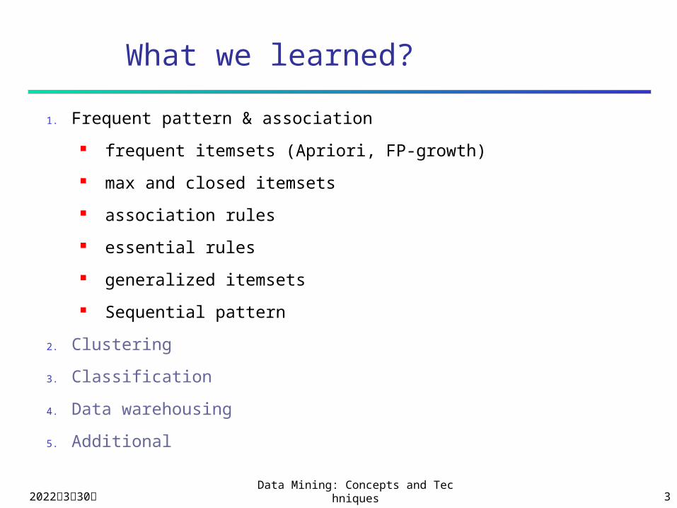
What we learned?
1. Frequent pattern & association
2. Clustering
3. Classification
4. Data warehousing
5. Additional
2023年4月18日Data Mining: Concepts and Technique
s 3
What we learned?
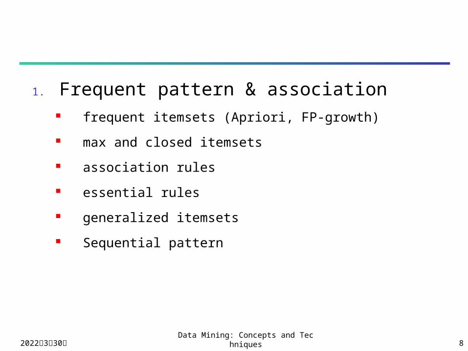
1. Frequent pattern & association
frequent itemsets (Apriori, FP-growth)
max and closed itemsets
association rules
essential rules
generalized itemsets
Sequential pattern
2. Clustering
3. Classification
4. Data warehousing
5. Additional

2023年4月18日Data Mining: Concepts and Technique
s 4
What we learned?
1. Frequent pattern & association
2. Clustering
k-means
Birch (based on CF-tree)
DBSCAN
CURE
3. Classification
4. Data warehousing
5. Additional

2023年4月18日Data Mining: Concepts and Technique
s 5
What we learned?
1. Frequent pattern & association
2. Clustering
3. Classification
decision tree
naïve Baysian classifier
Baysian network
neural net and SVM
4. Data warehousing
5. Additional
2023年4月18日Data Mining: Concepts and Technique
s 6
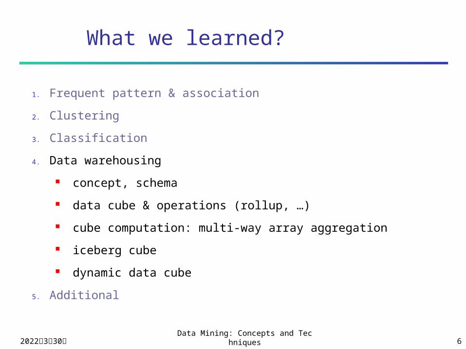
What we learned?
1. Frequent pattern & association
2. Clustering
3. Classification
4. Data warehousing
concept, schema
data cube & operations (rollup, …)
cube computation: multi-way array aggregation
iceberg cube
dynamic data cube
5. Additional
2023年4月18日Data Mining: Concepts and Technique
s 7
What we learned?
1. Frequent pattern & association
2. Clustering
3. Classification
4. Data warehousing
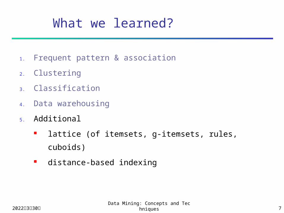
5. Additional
lattice (of itemsets, g-itemsets, rules, cuboids)
distance-based indexing
2023年4月18日Data Mining: Concepts and Technique
s 8
1. Frequent pattern & association frequent itemsets (Apriori, FP-growth)
max and closed itemsets
association rules
essential rules
generalized itemsets
Sequential pattern
2023年4月18日Data Mining: Concepts and Technique
s 9
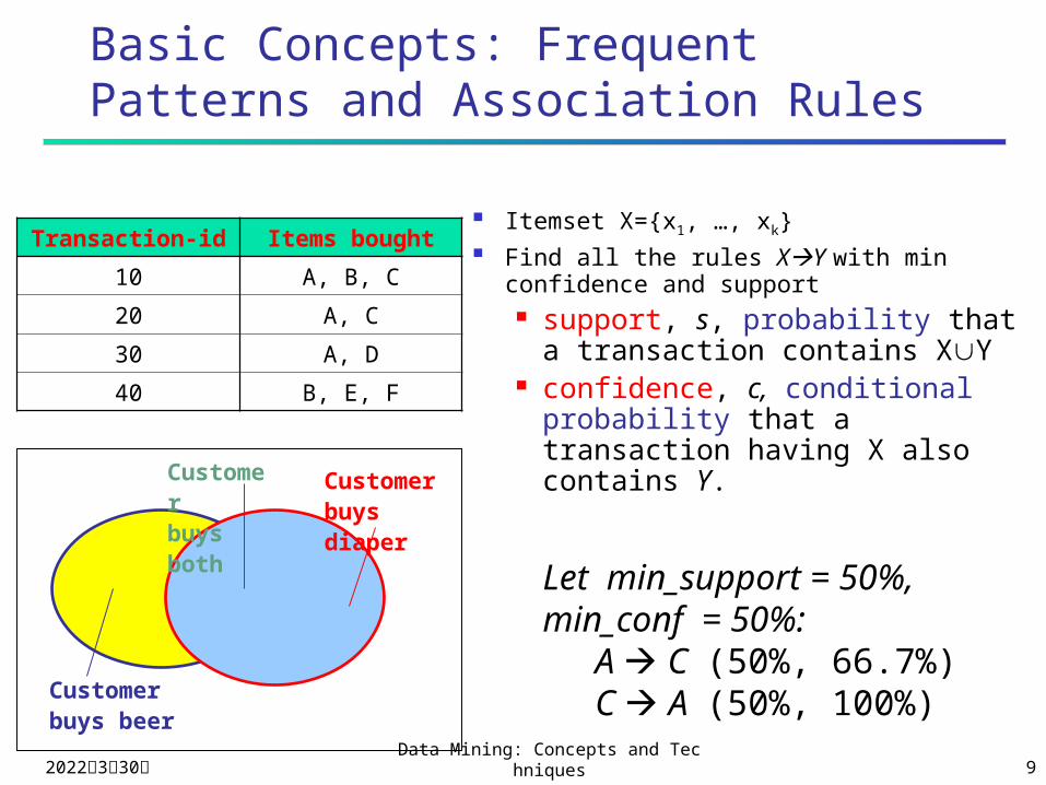
Basic Concepts: Frequent Patterns and Association Rules
Itemset X={x1, …, xk} Find all the rules XY with min
confidence and support support, s, probability that a
transaction contains XY confidence, c, conditional
probability that a transaction having X also contains Y.
Let min_support = 50%, min_conf = 50%:
A C (50%, 66.7%)C A (50%, 100%)
Customerbuys diaper
Customerbuys both
Customerbuys beer
Transaction-id Items bought
10 A, B, C
20 A, C
30 A, D
40 B, E, F
2023年4月18日Data Mining: Concepts and Technique
s 10
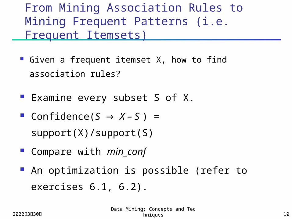
From Mining Association Rules to Mining Frequent Patterns (i.e. Frequent Itemsets)
Given a frequent itemset X, how to find association
rules?
Examine every subset S of X.
Confidence(S X – S ) = support(X)/support(S)
Compare with min_conf
An optimization is possible (refer to exercises
6.1, 6.2).

2023年4月18日Data Mining: Concepts and Technique
s 11
The Apriori Algorithm—An Example
Database TDB
1st scan
C1L1
L2
C2 C2
2nd scan
C3 L33rd scan
Tid Items
10 A, C, D
20 B, C, E
30 A, B, C, E
40 B, E
Itemset sup
{A} 2
{B} 3
{C} 3
{D} 1
{E} 3
Itemset sup
{A} 2
{B} 3
{C} 3
{E} 3
Itemset
{A, B}
{A, C}
{A, E}
{B, C}
{B, E}
{C, E}
Itemset sup{A, B} 1{A, C} 2{A, E} 1{B, C} 2{B, E} 3{C, E} 2
Itemset sup{A, C} 2{B, C} 2{B, E} 3{C, E} 2
Itemset
{B, C, E}Itemset sup{B, C, E} 2
2023年4月18日Data Mining: Concepts and Technique
s 12
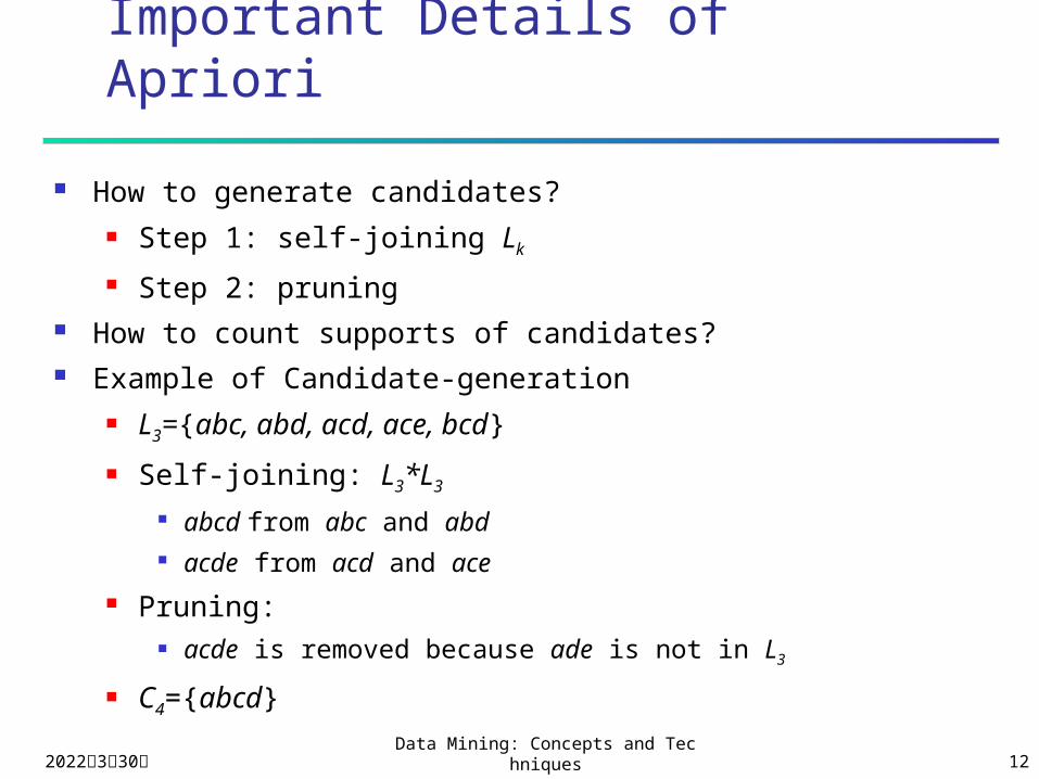
Important Details of Apriori
How to generate candidates? Step 1: self-joining Lk
Step 2: pruning How to count supports of candidates? Example of Candidate-generation
L3={abc, abd, acd, ace, bcd}
Self-joining: L3*L3
abcd from abc and abd acde from acd and ace
Pruning: acde is removed because ade is not in L3
C4={abcd}

2023年4月18日Data Mining: Concepts and Technique
s 13
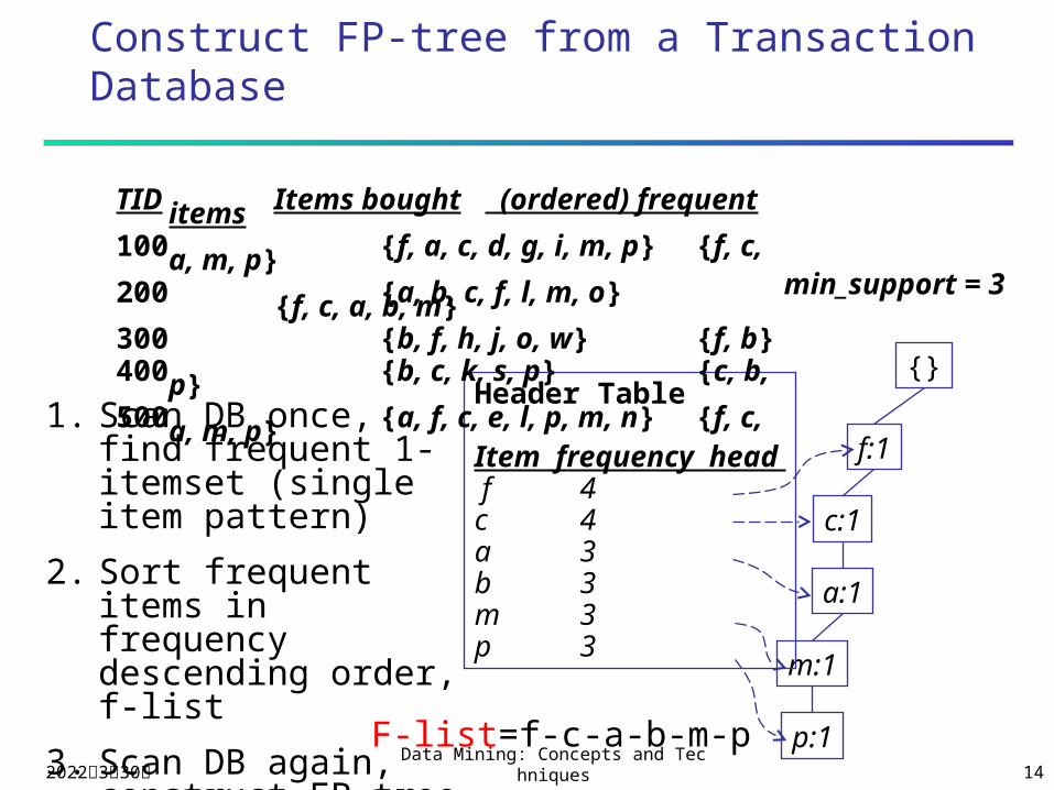
Construct FP-tree from a Transaction Database
Header Table
Item frequency head f 4c 4a 3b 3m 3p 3
min_support = 3
TID Items bought (ordered) frequent items100 {f, a, c, d, g, i, m, p} {f, c, a, m, p}200 {a, b, c, f, l, m, o} {f, c, a, b, m}300 {b, f, h, j, o, w} {f, b}400 {b, c, k, s, p} {c, b, p}500 {a, f, c, e, l, p, m, n} {f, c, a, m, p}
1. Scan DB once, find frequent 1-itemset (single item pattern)
2. Sort frequent items in frequency descending order, f-list
3. Scan DB again, construct FP-tree F-list=f-c-a-b-m-p
2023年4月18日Data Mining: Concepts and Technique
s 14
Construct FP-tree from a Transaction Database
{}
f:1
c:1
a:1
m:1
p:1
Header Table
Item frequency head f 4c 4a 3b 3m 3p 3
min_support = 3
TID Items bought (ordered) frequent items100 {f, a, c, d, g, i, m, p} {f, c, a, m, p}200 {a, b, c, f, l, m, o} {f, c, a, b, m}300 {b, f, h, j, o, w} {f, b}400 {b, c, k, s, p} {c, b, p}500 {a, f, c, e, l, p, m, n} {f, c, a, m, p}
1. Scan DB once, find frequent 1-itemset (single item pattern)
2. Sort frequent items in frequency descending order, f-list
3. Scan DB again, construct FP-tree F-list=f-c-a-b-m-p
2023年4月18日Data Mining: Concepts and Technique
s 15
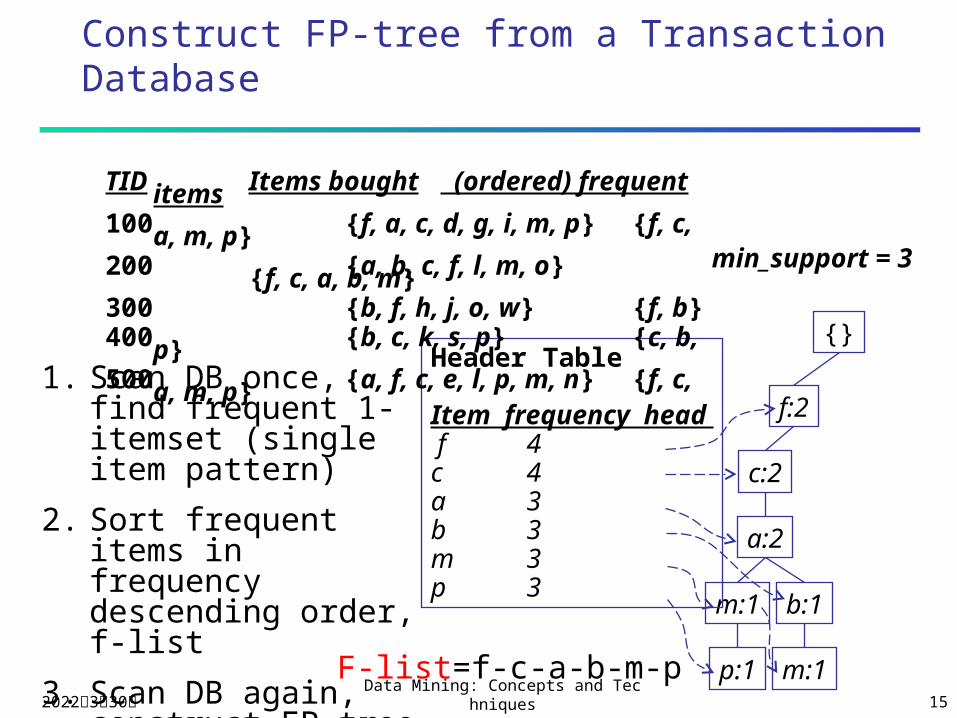
Construct FP-tree from a Transaction Database
{}
f:2
c:2
a:2
b:1m:1
p:1 m:1
Header Table
Item frequency head f 4c 4a 3b 3m 3p 3
min_support = 3
TID Items bought (ordered) frequent items100 {f, a, c, d, g, i, m, p} {f, c, a, m, p}200 {a, b, c, f, l, m, o} {f, c, a, b, m}300 {b, f, h, j, o, w} {f, b}400 {b, c, k, s, p} {c, b, p}500 {a, f, c, e, l, p, m, n} {f, c, a, m, p}
1. Scan DB once, find frequent 1-itemset (single item pattern)
2. Sort frequent items in frequency descending order, f-list
3. Scan DB again, construct FP-tree F-list=f-c-a-b-m-p
2023年4月18日Data Mining: Concepts and Technique
s 16
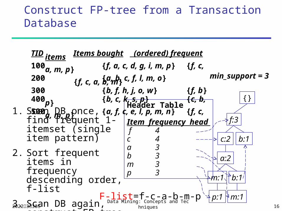
Construct FP-tree from a Transaction Database
{}
f:3
c:2
a:2
b:1m:1
p:1 m:1
Header Table
Item frequency head f 4c 4a 3b 3m 3p 3
min_support = 3
TID Items bought (ordered) frequent items100 {f, a, c, d, g, i, m, p} {f, c, a, m, p}200 {a, b, c, f, l, m, o} {f, c, a, b, m}300 {b, f, h, j, o, w} {f, b}400 {b, c, k, s, p} {c, b, p}500 {a, f, c, e, l, p, m, n} {f, c, a, m, p}
1. Scan DB once, find frequent 1-itemset (single item pattern)
2. Sort frequent items in frequency descending order, f-list
3. Scan DB again, construct FP-tree F-list=f-c-a-b-m-p
b:1

2023年4月18日Data Mining: Concepts and Technique
s 17
Construct FP-tree from a Transaction Database
{}
f:3 c:1
b:1
p:1
b:1c:2
a:2
b:1m:1
p:1 m:1
Header Table
Item frequency head f 4c 4a 3b 3m 3p 3
min_support = 3
TID Items bought (ordered) frequent items100 {f, a, c, d, g, i, m, p} {f, c, a, m, p}200 {a, b, c, f, l, m, o} {f, c, a, b, m}300 {b, f, h, j, o, w} {f, b}400 {b, c, k, s, p} {c, b, p}500 {a, f, c, e, l, p, m, n} {f, c, a, m, p}
1. Scan DB once, find frequent 1-itemset (single item pattern)
2. Sort frequent items in frequency descending order, f-list
3. Scan DB again, construct FP-tree F-list=f-c-a-b-m-p

2023年4月18日Data Mining: Concepts and Technique
s 18
Construct FP-tree from a Transaction Database
{}
f:4 c:1
b:1
p:1
b:1c:3
a:3
b:1m:2
p:2 m:1
Header Table
Item frequency head f 4c 4a 3b 3m 3p 3
min_support = 3
TID Items bought (ordered) frequent items100 {f, a, c, d, g, i, m, p} {f, c, a, m, p}200 {a, b, c, f, l, m, o} {f, c, a, b, m}300 {b, f, h, j, o, w} {f, b}400 {b, c, k, s, p} {c, b, p}500 {a, f, c, e, l, p, m, n} {f, c, a, m, p}
1. Scan DB once, find frequent 1-itemset (single item pattern)
2. Sort frequent items in frequency descending order, f-list
3. Scan DB again, construct FP-tree F-list=f-c-a-b-m-p
2023年4月18日Data Mining: Concepts and Technique
s 19
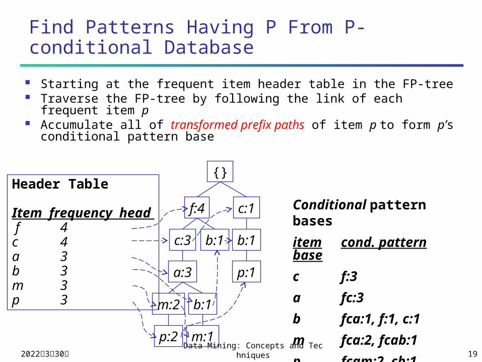
Find Patterns Having P From P-conditional Database
Starting at the frequent item header table in the FP-tree Traverse the FP-tree by following the link of each frequent
item p Accumulate all of transformed prefix paths of item p to
form p’s conditional pattern base
Conditional pattern bases
item cond. pattern base
c f:3
a fc:3
b fca:1, f:1, c:1
m fca:2, fcab:1
p fcam:2, cb:1
{}
f:4 c:1
b:1
p:1
b:1c:3
a:3
b:1m:2
p:2 m:1
Header Table
Item frequency head f 4c 4a 3b 3m 3p 3
2023年4月18日Data Mining: Concepts and Technique
s 20
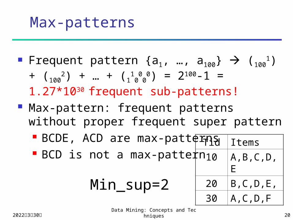
Max-patterns
Frequent pattern {a1, …, a100} (1001) +
(1002) + … + (1
10
00
0) = 2100-1 = 1.27*1030
frequent sub-patterns! Max-pattern: frequent patterns without
proper frequent super pattern BCDE, ACD are max-patterns BCD is not a max-pattern
Tid Items
10 A,B,C,D,E
20 B,C,D,E,
30 A,C,D,FMin_sup=2
2023年4月18日Data Mining: Concepts and Technique
s 21
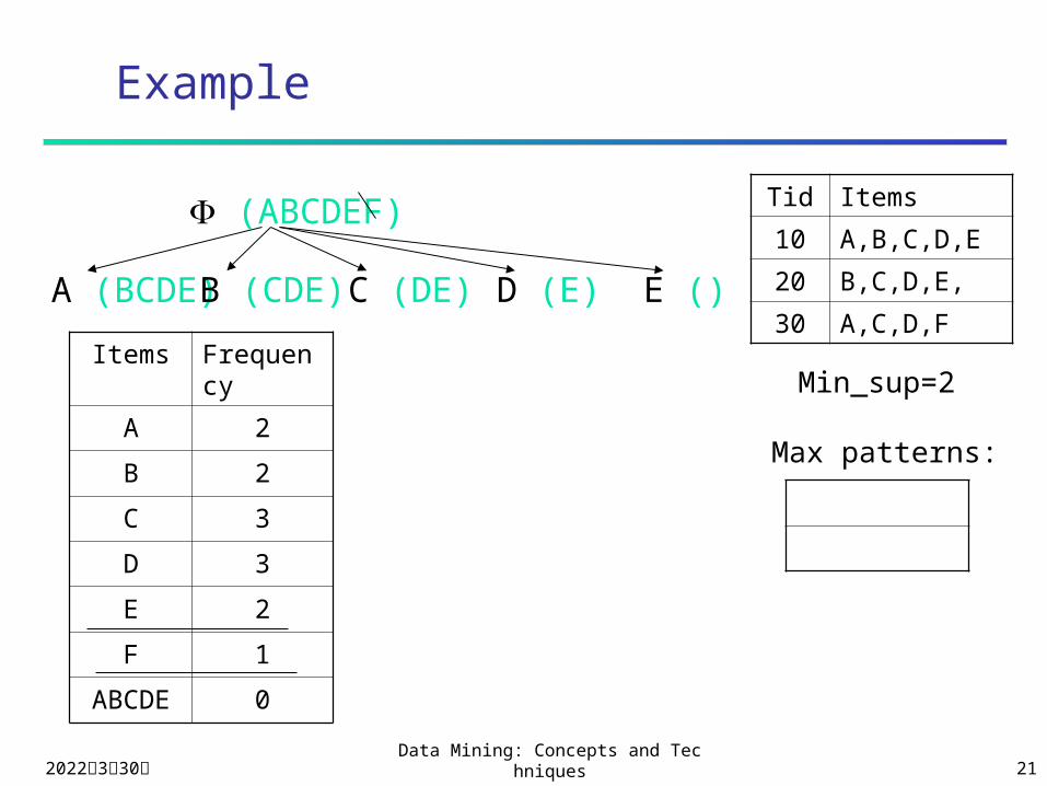
Example
Tid Items
10 A,B,C,D,E
20 B,C,D,E,
30 A,C,D,F
(ABCDEF)
Items Frequency
A 2
B 2
C 3
D 3
E 2
F 1
ABCDE 0
Min_sup=2
Max patterns:
A (BCDE)B (CDE) C (DE) E ()D (E)

2023年4月18日Data Mining: Concepts and Technique
s 22
Example
Tid Items
10 A,B,C,D,E
20 B,C,D,E,
30 A,C,D,F
Items Frequency
AB 1
AC 2
AD 2
AE 1
ACD 2
Min_sup=2
(ABCDEF)
A (BCDE)B (CDE) C (DE) E ()D (E)
Max patterns:
Node A
2023年4月18日Data Mining: Concepts and Technique
s 23
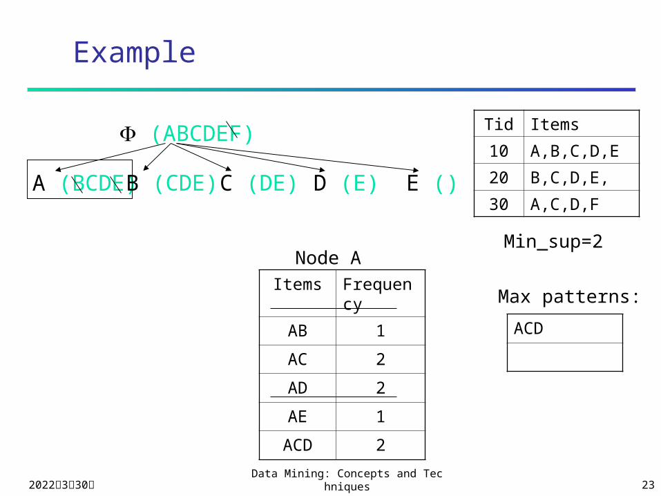
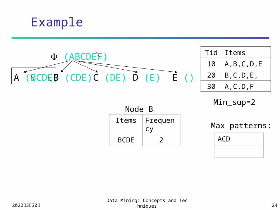
Example
Tid Items
10 A,B,C,D,E
20 B,C,D,E,
30 A,C,D,F
Items Frequency
AB 1
AC 2
AD 2
AE 1
ACD 2
Min_sup=2
(ABCDEF)
A (BCDE)B (CDE) C (DE) E ()D (E)
ACD
Max patterns:
Node A
2023年4月18日Data Mining: Concepts and Technique
s 24
Example
Tid Items
10 A,B,C,D,E
20 B,C,D,E,
30 A,C,D,F
Items Frequency
BCDE 2
Min_sup=2
(ABCDEF)
A (BCDE)B (CDE) C (DE) E ()D (E)
ACD
Max patterns:
Node B
2023年4月18日Data Mining: Concepts and Technique
s 25
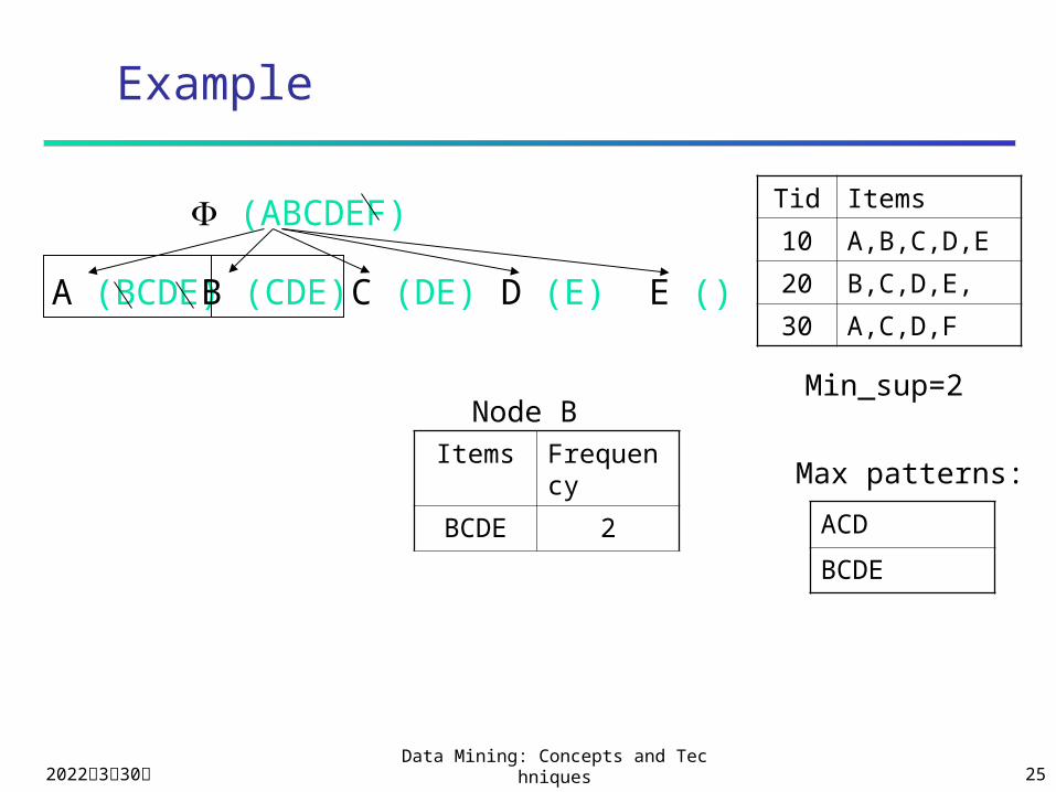
Example
Tid Items
10 A,B,C,D,E
20 B,C,D,E,
30 A,C,D,F
Items Frequency
BCDE 2
Min_sup=2
(ABCDEF)
A (BCDE)B (CDE) C (DE) E ()D (E)
ACD
BCDE
Max patterns:
Node B
2023年4月18日Data Mining: Concepts and Technique
s 26
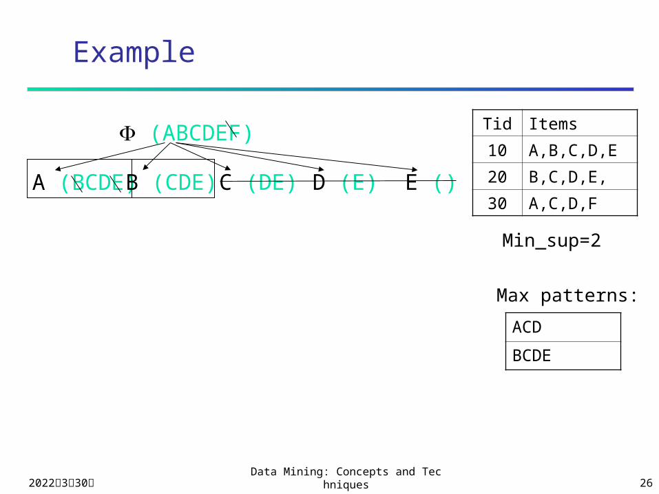
Example
Tid Items
10 A,B,C,D,E
20 B,C,D,E,
30 A,C,D,F
Min_sup=2
(ABCDEF)
A (BCDE)B (CDE) C (DE) E ()D (E)
ACD
BCDE
Max patterns:
2023年4月18日Data Mining: Concepts and Technique
s 27
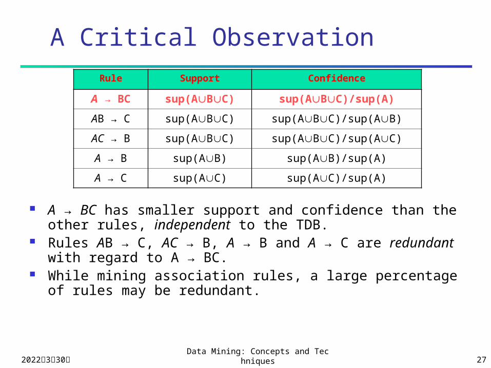
A Critical Observation
Rule Support Confidence
A → BC sup(ABC) sup(ABC)/sup(A)
AB → C sup(ABC) sup(ABC)/sup(AB)
AC → B sup(ABC) sup(ABC)/sup(AC)
A → B sup(AB) sup(AB)/sup(A)
A → C sup(AC) sup(AC)/sup(A)
A → BC has smaller support and confidence than the other rules, independent to the TDB.
Rules AB → C, AC → B, A → B and A → C are redundant with regard to A → BC.
While mining association rules, a large percentage of rules may be redundant.
2023年4月18日Data Mining: Concepts and Technique
s 28
Formal Definition of Essential Rule
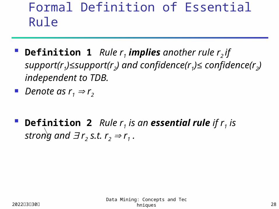
Definition 1 Rule r1 implies another rule r2 if support(r1)≤support(r2) and confidence(r1)≤ confidence(r2) independent to TDB.
Denote as r1 r2
Definition 2 Rule r1 is an essential rule if r1 is strong and r2 s.t. r2 r1 .

2023年4月18日Data Mining: Concepts and Technique
s 29
Example of a Lattice of rules
ABC
ABCCABBAC
ACBABCABAC BABC BCA CACB
• Generate the child nodes: move or delete from the consequent.• To find essential rules: start from each max itemset; browse top-down; prune a sub-tree whenever a rule is confident.
2023年4月18日Data Mining: Concepts and Technique
s 30
Frequent generalized itemsets
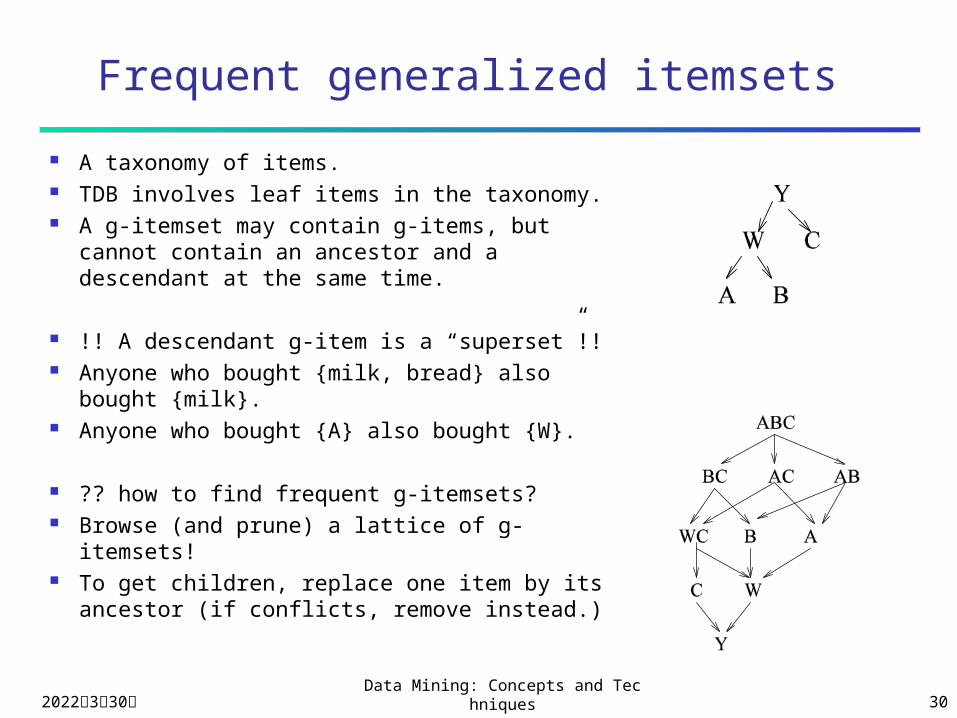
A taxonomy of items. TDB involves leaf items in the taxonomy. A g-itemset may contain g-items, but
cannot contain an ancestor and a descendant at the same time.
!! A descendant g-item is a “superset”!! Anyone who bought {milk, bread} also
bought {milk}. Anyone who bought {A} also bought {W}.
?? how to find frequent g-itemsets? Browse (and prune) a lattice of g-
itemsets! To get children, replace one item by its
ancestor (if conflicts, remove instead.)

2023年4月18日Data Mining: Concepts and Technique
s 31
What Is Sequential Pattern Mining?
Given a set of sequences, find the complete set of frequent subsequences
A sequence database Given support threshold min_sup =2, <(ab)c> is a sequential pattern
SID sequence
10 <a(abc)(ac)d(cf)>
20 <(ad)c(bc)(ae)>
30 <(ef)(ab)(df)cb>
40 <eg(af)cbc>

2023年4月18日Data Mining: Concepts and Technique
s 32
Mining Sequential Patterns by Prefix Projections
Step 1: find length-1 sequential patterns <a>, <b>, <c>, <d>, <e>, <f>
Step 2: divide search space. The complete set of seq. pat. can be partitioned into 6 subsets: The ones having prefix <a>; The ones having prefix <b>; … The ones having prefix <f>
SID sequence
10 <a(abc)(ac)d(cf)>
20 <(ad)c(bc)(ae)>
30 <(ef)(ab)(df)cb>
40 <eg(af)cbc>

2023年4月18日Data Mining: Concepts and Technique
s 33
Finding Seq. Patterns with Prefix <a>
Only need to consider projections w.r.t. <a> <a>-projected database: <(abc)(ac)d(cf)>,
<(_d)c(bc)(ae)>, <(_b)(df)cb>, <(_f)cbc>
Find all the length-2 seq. pat. Having prefix <a>: <aa>, <ab>, <(ab)>, <ac>, <ad>, <af>,
by checking the frequency of items like a and _a. Further partition into 6 subsets
Having prefix <aa>; … Having prefix <af>
SID sequence
10 <a(abc)(ac)d(cf)>
20 <(ad)c(bc)(ae)>
30 <(ef)(ab)(df)cb>
40 <eg(af)cbc>

2023年4月18日Data Mining: Concepts and Technique
s 34
2. Clustering k-means
Birch (based on CF-tree)
DBSCAN
CURE

2023年4月18日Data Mining: Concepts and Technique
s 35
The K-Means Clustering Method
Pick k objects as initial seed points Assign each object to the cluster with the
nearest seed point Re-compute each seed point as the
centroid (or mean point) of its cluster Go back to Step 2, stop when no more new
assignment
Not optimal. A counter example?

2023年4月18日Data Mining: Concepts and Technique
s 36
BIRCH (1996)
Birch: Balanced Iterative Reducing and Clustering using Hierarchies, by Zhang, Ramakrishnan, Livny (SIGMOD’96)
Incrementally construct a CF (Clustering Feature) tree, a hierarchical data structure for multiphase clustering Phase 1: scan DB to build an initial in-memory CF tree
(a multi-level compression of the data that tries to preserve the inherent clustering structure of the data)
Phase 2: use an arbitrary clustering algorithm to cluster the leaf nodes of the CF-tree
Scales linearly: finds a good clustering with a single scan and improves the quality with a few additional scans
Weakness: handles only numeric data, and sensitive to the order of the data record.
Balanced Iterative Reducing and Clustering using Hierarchies
2023年4月18日Data Mining: Concepts and Technique
s 37
Clustering Feature Vector
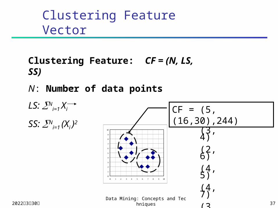
Clustering Feature: CF = (N, LS, SS)
N: Number of data points
LS: Ni=1 Xi
SS: Ni=1 (Xi )2
0
1
2
3
4
5
6
7
8
9
10
0 1 2 3 4 5 6 7 8 9 10
CF = (5, (16,30),244)
(3,4)(2,6)(4,5)(4,7)(3,8)

2023年4月18日Data Mining: Concepts and Technique
s 38
Some Characteristics of CF
Two CF can be aggregated.
Given CF1=(N1, LS1, SS1), CF2 = (N2, LS2, SS2),
If combined into one cluster, CF=(N1+N2, LS1+LS2, SS1+SS2).
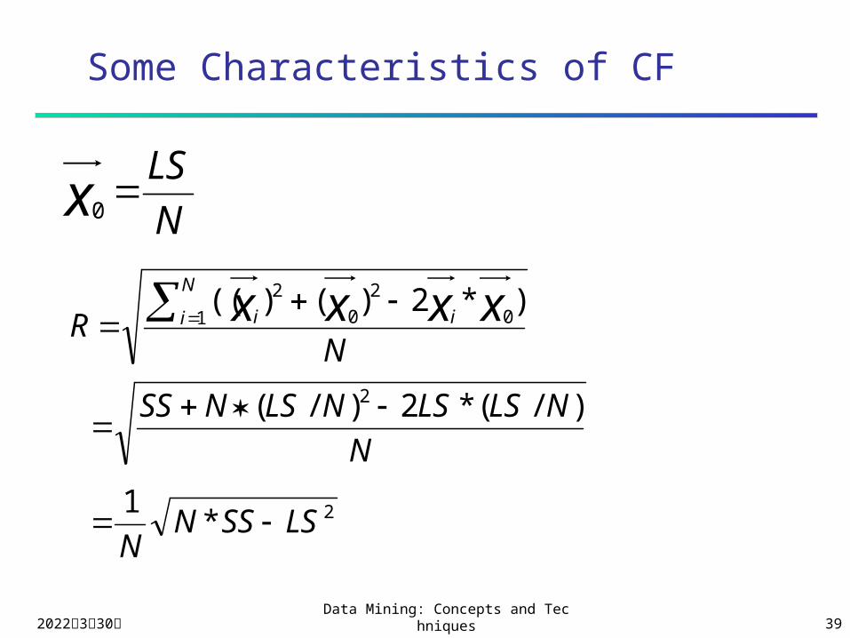
The centroid and radius can both be computed from CF.
centroid is the center of the cluster
radius is the average distance between an object and the centroid.
how?
N
N
i ixx 1
0N
R
N
i i xx 2
1 0)(
2023年4月18日Data Mining: Concepts and Technique
s 39
Some Characteristics of CF
N
LSx
0
N
NLSLSNLSNSS )/(*2)/( 2
NR xxxx i
N
i i)*2)()((
0
2
1 0
2
2*1
LSSSNN
2023年4月18日Data Mining: Concepts and Technique
s 40
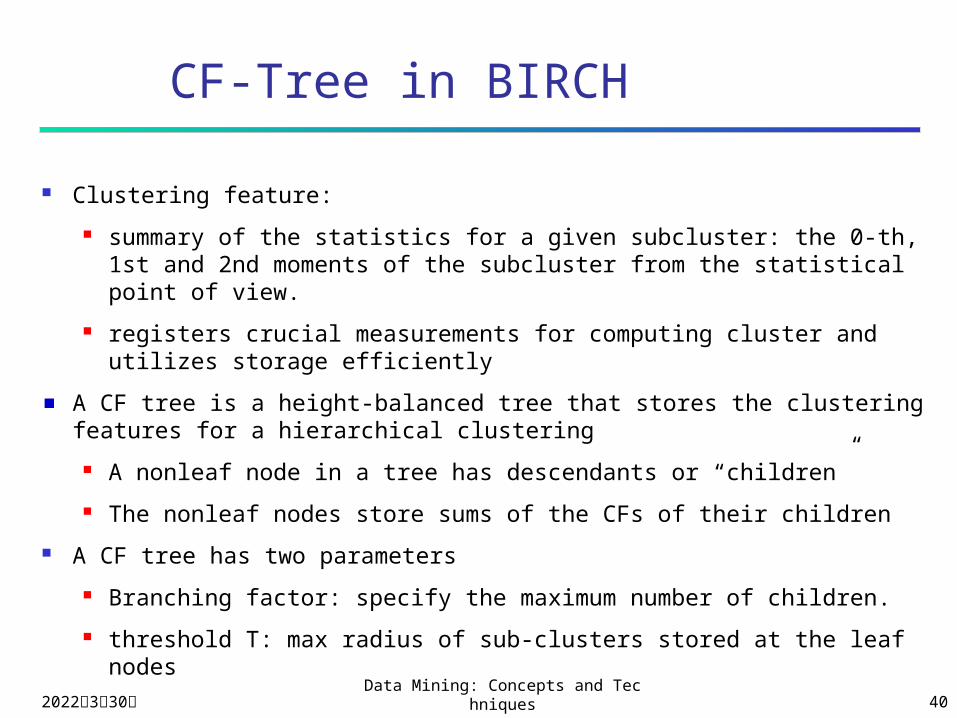
CF-Tree in BIRCH
Clustering feature:
summary of the statistics for a given subcluster: the 0-th, 1st and 2nd moments of the subcluster from the statistical point of view.
registers crucial measurements for computing cluster and utilizes storage efficiently
A CF tree is a height-balanced tree that stores the clustering features for a hierarchical clustering
A nonleaf node in a tree has descendants or “children”
The nonleaf nodes store sums of the CFs of their children
A CF tree has two parameters
Branching factor: specify the maximum number of children.
threshold T: max radius of sub-clusters stored at the leaf nodes

2023年4月18日Data Mining: Concepts and Technique
s 41
Insertion in a CF-Tree
To insert an object o to a CF-tree, insert to the root node of the CF-tree.
To insert o into an index node, insert into the child node whose centroid is the closest to o.
To insert o into a leaf node,
If an existing leaf entry can “absorb” it (i.e. new radius <= T), let it be;
Otherwise, create a new leaf entry.
Split:
Choose two entries whose centroids are the farthest away;
Assign them to two different groups;
Assign the remaining entries to one of these groups.
2023年4月18日Data Mining: Concepts and Technique
s 42
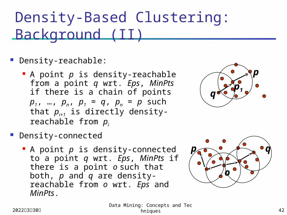
Density-Based Clustering: Background (II)
Density-reachable: A point p is density-reachable
from a point q wrt. Eps, MinPts if there is a chain of points p1, …, pn, p1 = q, pn = p such that pi+1 is directly density-reachable from pi
Density-connected A point p is density-connected to
a point q wrt. Eps, MinPts if there is a point o such that both, p and q are density-reachable from o wrt. Eps and MinPts.
p
qp1
p q
o
2023年4月18日Data Mining: Concepts and Technique
s 43
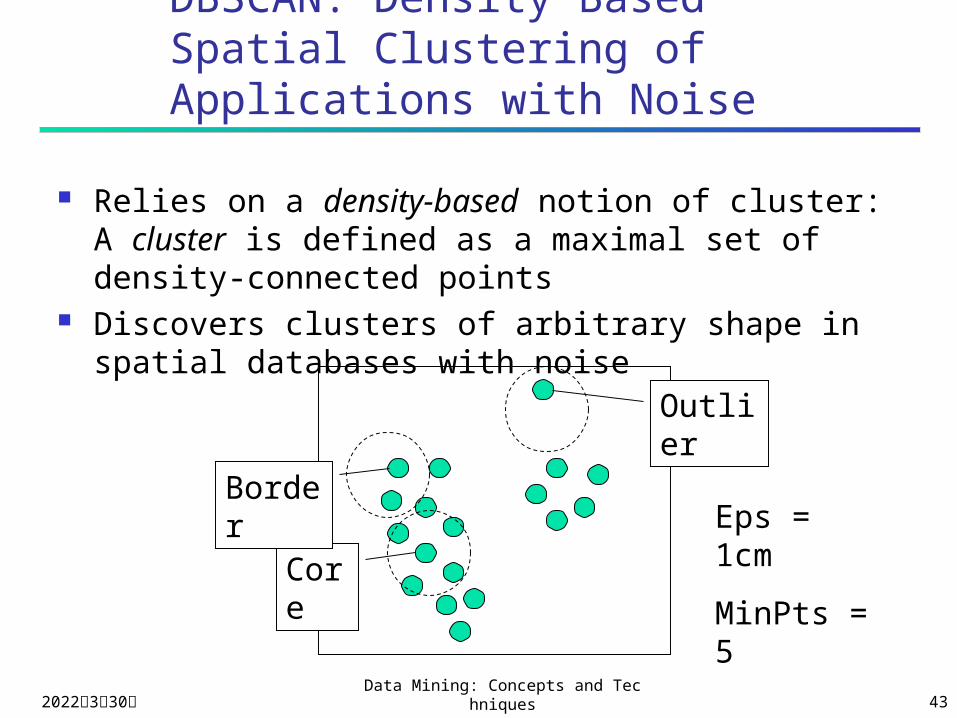
DBSCAN: Density Based Spatial Clustering of Applications with Noise
Relies on a density-based notion of cluster: A cluster is defined as a maximal set of density-connected points
Discovers clusters of arbitrary shape in spatial databases with noise
Core
Border
Outlier
Eps = 1cm
MinPts = 5
2023年4月18日Data Mining: Concepts and Technique
s 44
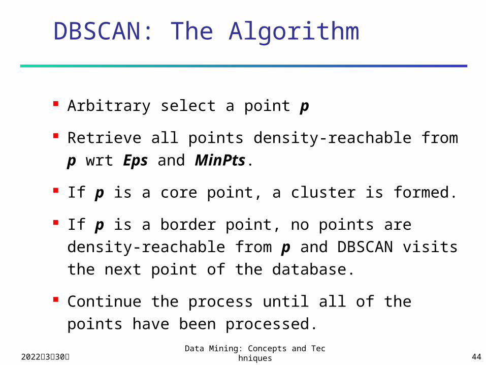
DBSCAN: The Algorithm
Arbitrary select a point p
Retrieve all points density-reachable from p wrt Eps and MinPts.
If p is a core point, a cluster is formed.
If p is a border point, no points are density-reachable from p and DBSCAN visits the next point of the database.
Continue the process until all of the points have been processed.
2023年4月18日Data Mining: Concepts and Technique
s 45
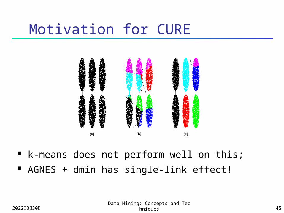
k-means does not perform well on this; AGNES + dmin has single-link effect!
Motivation for CURE
2023年4月18日Data Mining: Concepts and Technique
s 46
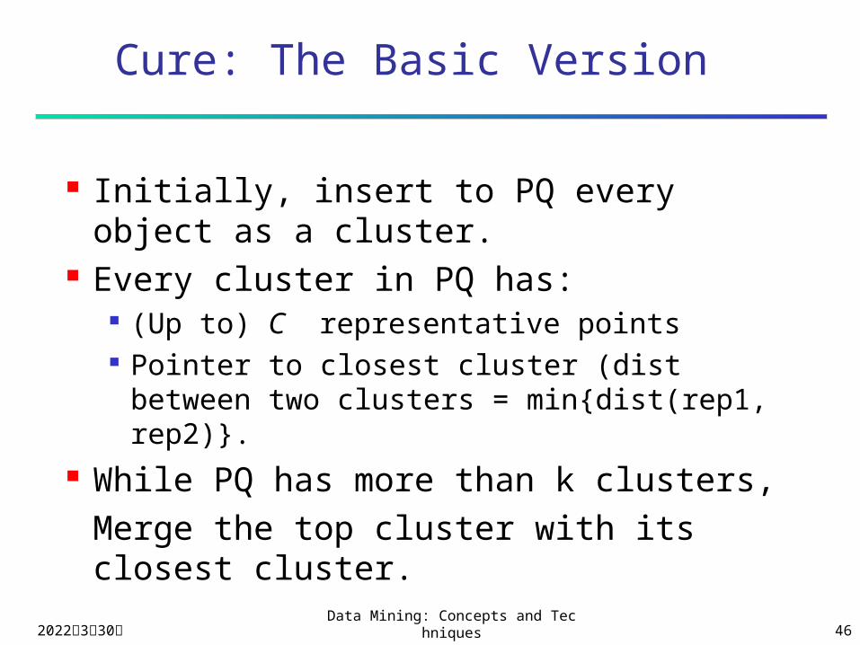
Cure: The Basic Version
Initially, insert to PQ every object as a cluster.
Every cluster in PQ has: (Up to) C representative points Pointer to closest cluster (dist between two
clusters = min{dist(rep1, rep2)}. While PQ has more than k clusters,
Merge the top cluster with its closest cluster.
2023年4月18日Data Mining: Concepts and Technique
s 47
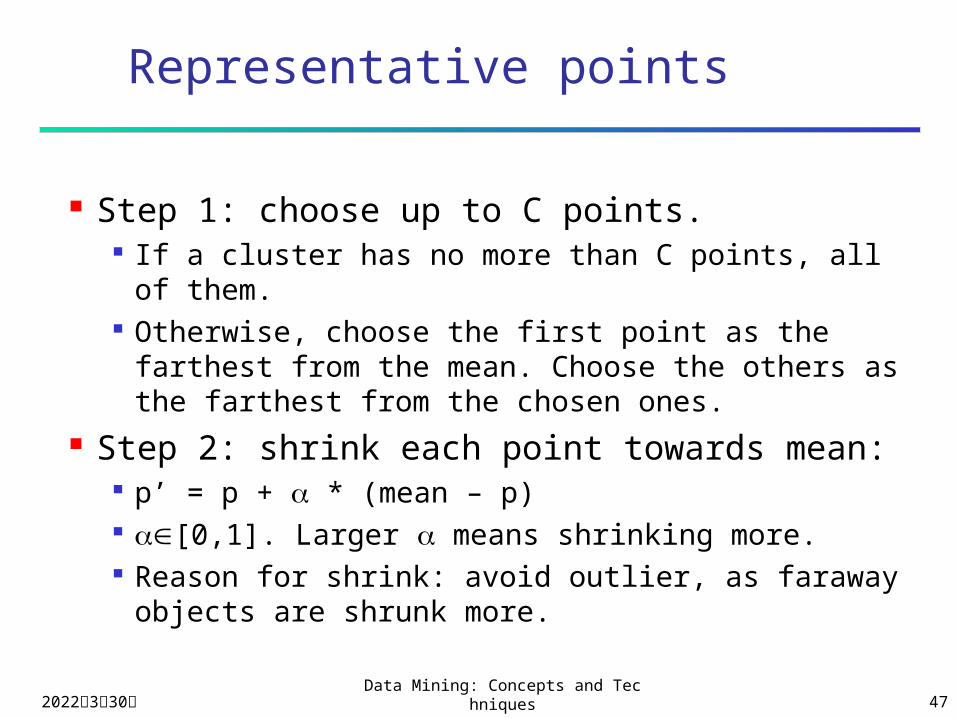
Representative points
Step 1: choose up to C points. If a cluster has no more than C points, all of them. Otherwise, choose the first point as the farthest
from the mean. Choose the others as the farthest from the chosen ones.
Step 2: shrink each point towards mean: p’ = p + * (mean – p) [0,1]. Larger means shrinking more. Reason for shrink: avoid outlier, as faraway
objects are shrunk more.
2023年4月18日Data Mining: Concepts and Technique
s 48
3. Classification decision tree
naïve Baysian classifier
Baysian net
neural net and SVM

2023年4月18日Data Mining: Concepts and Technique
s 49
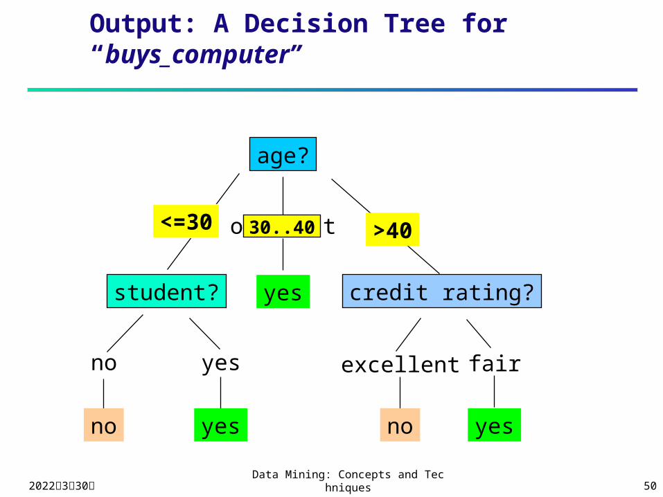
Training Dataset
age income student credit_rating buys_computer<=30 high no fair no<=30 high no excellent no31…40 high no fair yes>40 medium no fair yes>40 low yes fair yes>40 low yes excellent no31…40 low yes excellent yes<=30 medium no fair no<=30 low yes fair yes>40 medium yes fair yes<=30 medium yes excellent yes31…40 medium no excellent yes31…40 high yes fair yes>40 medium no excellent no
This follows an example from Quinlan’s ID3
2023年4月18日Data Mining: Concepts and Technique
s 50
Output: A Decision Tree for “buys_computer”
age?
overcast
student? credit rating?
no yes fairexcellent
<=30 >40
no noyes yes
yes
30..40
2023年4月18日Data Mining: Concepts and Technique
s 51
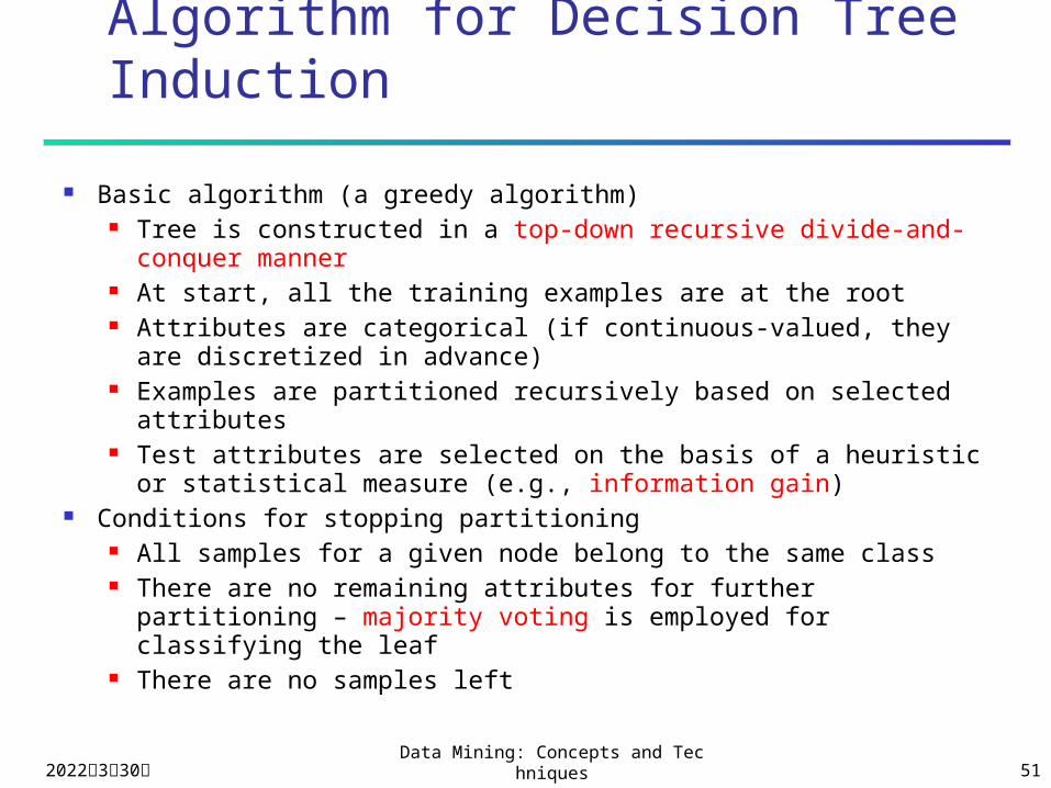
Algorithm for Decision Tree Induction
Basic algorithm (a greedy algorithm) Tree is constructed in a top-down recursive divide-and-
conquer manner At start, all the training examples are at the root Attributes are categorical (if continuous-valued, they are
discretized in advance) Examples are partitioned recursively based on selected
attributes Test attributes are selected on the basis of a heuristic or
statistical measure (e.g., information gain) Conditions for stopping partitioning
All samples for a given node belong to the same class There are no remaining attributes for further partitioning –
majority voting is employed for classifying the leaf There are no samples left
2023年4月18日Data Mining: Concepts and Technique
s 52
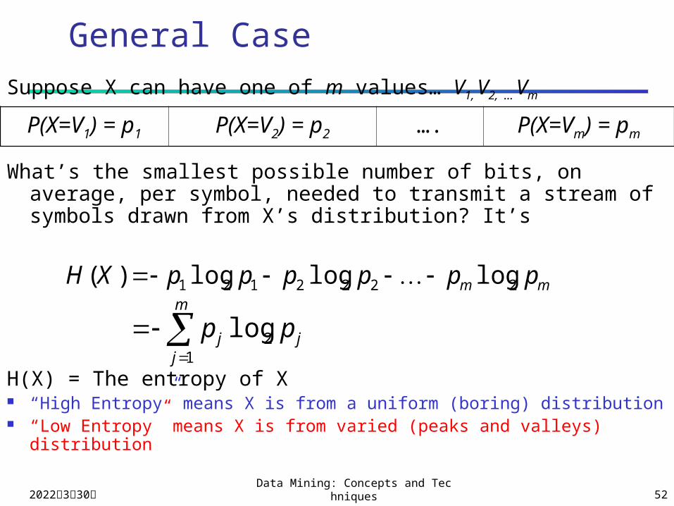
Suppose X can have one of m values… V1, V2, … Vm
What’s the smallest possible number of bits, on average, per symbol, needed to transmit a stream of symbols drawn from X’s distribution? It’s
H(X) = The entropy of X “High Entropy” means X is from a uniform (boring) distribution “Low Entropy” means X is from varied (peaks and valleys)
distribution
General Case
mm ppppppXH 2222121 logloglog)(
P(X=V1) = p1 P(X=V2) = p2 …. P(X=Vm) = pm
m
jjj pp
12log
2023年4月18日Data Mining: Concepts and Technique
s 53
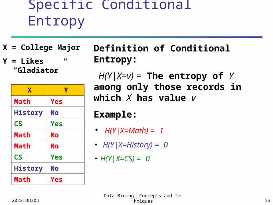
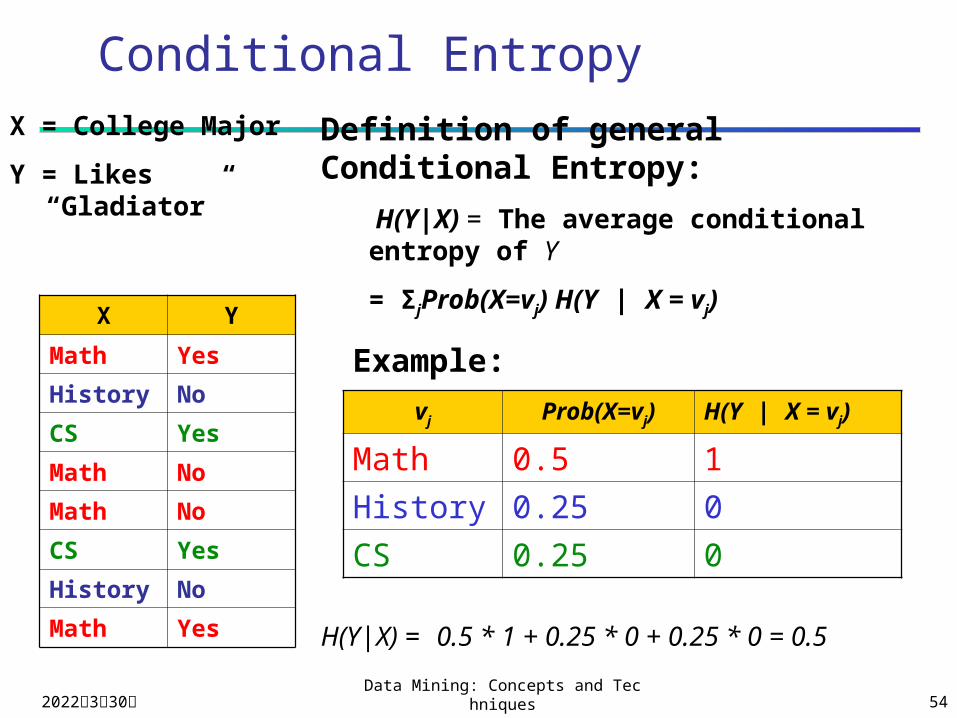
Specific Conditional Entropy
Definition of Conditional Entropy:
H(Y|X=v) = The entropy of Y among only those records in which X has value v
Example:
• H(Y|X=Math) = 1
• H(Y|X=History) = 0
• H(Y|X=CS) = 0
X = College Major
Y = Likes “Gladiator”
X Y
Math Yes
History No
CS Yes
Math No
Math No
CS Yes
History No
Math Yes
2023年4月18日Data Mining: Concepts and Technique
s 54
Conditional EntropyDefinition of general Conditional Entropy:
H(Y|X) = The average conditional entropy of Y
= ΣjProb(X=vj) H(Y | X = vj)
X = College Major
Y = Likes “Gladiator”
Example:
vj Prob(X=vj) H(Y | X = vj)
Math 0.5 1
History 0.25 0
CS 0.25 0
H(Y|X) = 0.5 * 1 + 0.25 * 0 + 0.25 * 0 = 0.5
X Y
Math Yes
History No
CS Yes
Math No
Math No
CS Yes
History No
Math Yes
2023年4月18日Data Mining: Concepts and Technique
s 55
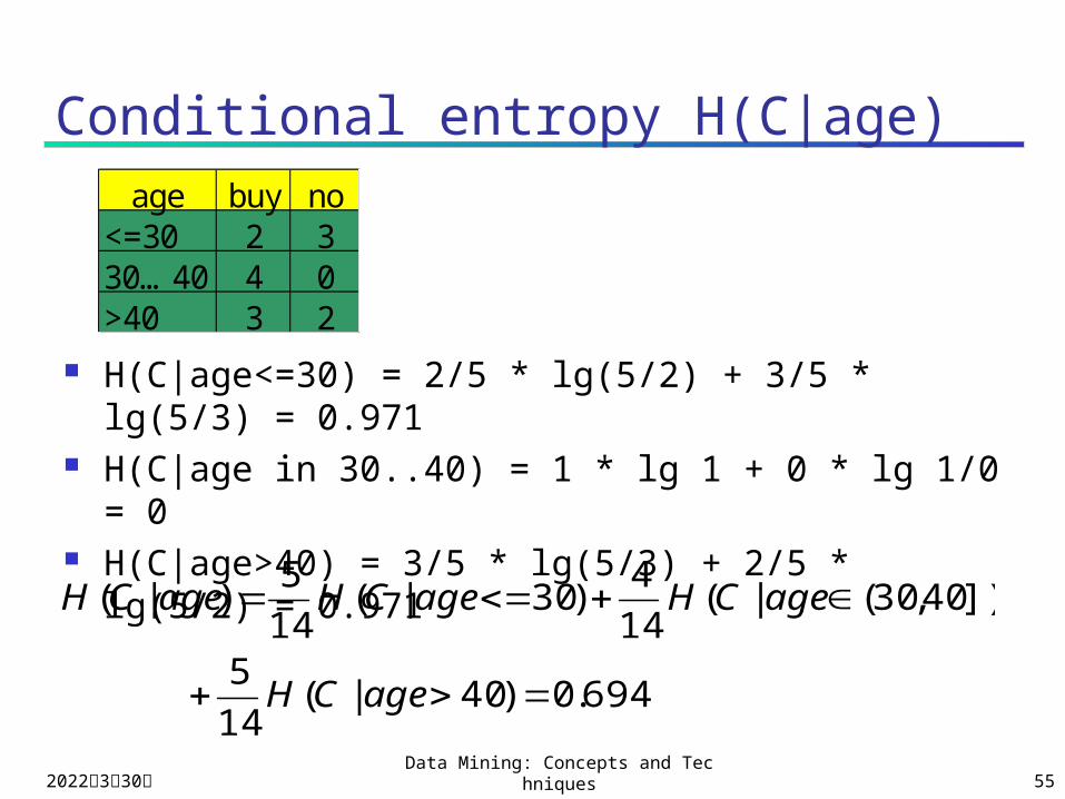
Conditional entropy H(C|age)
H(C|age<=30) = 2/5 * lg(5/2) + 3/5 * lg(5/3) = 0.971
H(C|age in 30..40) = 1 * lg 1 + 0 * lg 1/0 = 0 H(C|age>40) = 3/5 * lg(5/3) + 2/5 * lg(5/2) =
0.971
age buy no<=30 2 330…40 4 0>40 3 2
694.0)40|(14
5
])40,30(|(14
4)30|(
14
5)|(
ageCH
ageCHageCHageCH
2023年4月18日Data Mining: Concepts and Technique
s 56
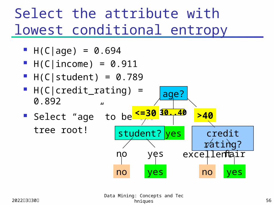
Select the attribute with lowest conditional entropy
H(C|age) = 0.694 H(C|income) = 0.911 H(C|student) = 0.789 H(C|credit_rating) =
0.892 Select “age” to be the
tree root! yes
age?
<=30 >4030..40
student?
no yes
no yes
credit rating?
fairexcellent
no yes
2023年4月18日Data Mining: Concepts and Technique
s 57
Bayesian Classification
X: a data sample whose class label is unknown, e.g. X =(Income=medium, Credit_rating=Fair, Age=40).
Hi: a hypothesis that a record belongs to class Ci, e.g.
Hi = a record belongs to the “buy computer” class. P(Hi), P(X): probabilities. P(Hi/X): a conditional probability: among all records
with medium income and fair credit rating, what’s the probability to buy a computer?
This is what we need for classification! Given X, P(Hi/X) tells us the possibility that it belongs to some class.
What if we need to determine a single class for X?
2023年4月18日Data Mining: Concepts and Technique
s 58
Bayesian Theorem
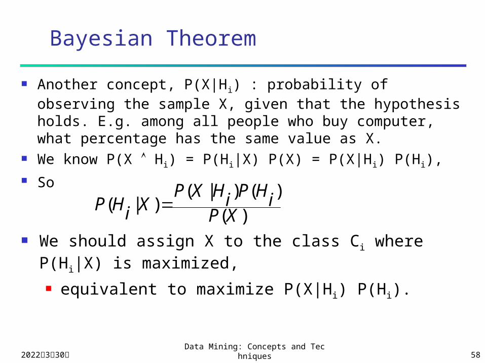
Another concept, P(X|Hi) : probability of observing the sample X, given that the hypothesis holds. E.g. among all people who buy computer, what percentage has the same value as X.
We know P(X Hi) = P(Hi|X) P(X) = P(X|Hi) P(Hi), So
)()()|(
)|(XP
iHPiHXPXiHP
We should assign X to the class Ci where P(Hi|X) is maximized, equivalent to maximize P(X|Hi) P(Hi).
2023年4月18日Data Mining: Concepts and Technique
s 59
Naïve Bayes Classifier
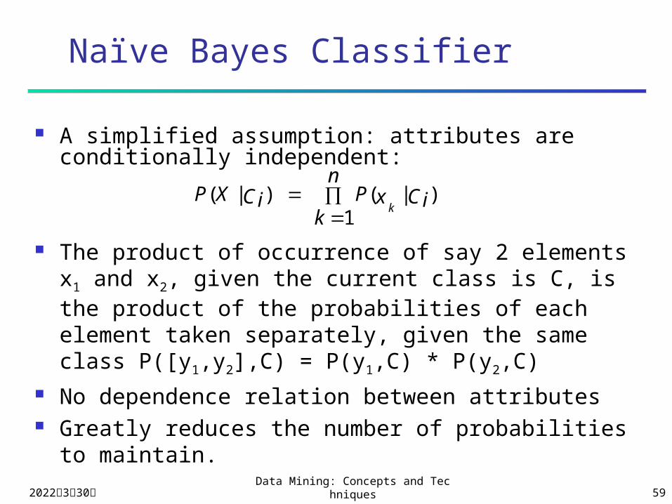
A simplified assumption: attributes are conditionally independent:
The product of occurrence of say 2 elements x1 and x2, given the current class is C, is the product of the probabilities of each element taken separately, given the same class P([y1,y2],C) = P(y1,C) * P(y2,C)
No dependence relation between attributes Greatly reduces the number of probabilities to
maintain.
n
kCixPCiXP
k1
)|()|(

2023年4月18日Data Mining: Concepts and Technique
s 60
Sample quiz questions
age income student credit_rating buys_computer<=30 high no fair no<=30 high no excellent no30…40 high no fair yes>40 medium no fair yes>40 low yes fair yes>40 low yes excellent no31…40 low yes excellent yes<=30 medium no fair no<=30 low yes fair yes>40 medium yes fair yes<=30 medium yes excellent yes31…40 medium no excellent yes31…40 high yes fair yes>40 medium no excellent no
1. What data does
naïve Baysian netmaintain?
2. Given X =(age<=30,Income=medium,Student=yesCredit_rating=Fai
r)
buy or not buy?
2023年4月18日Data Mining: Concepts and Technique
s 61
Naïve Bayesian Classifier: Example
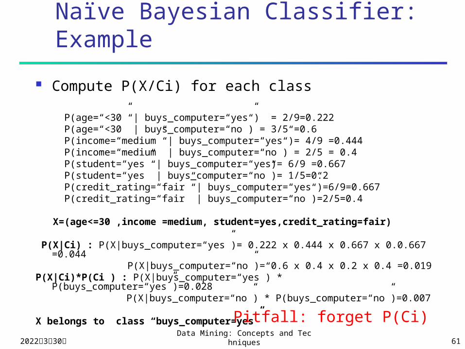
Compute P(X/Ci) for each class
P(age=“<30” | buys_computer=“yes”) = 2/9=0.222 P(age=“<30” | buys_computer=“no”) = 3/5 =0.6 P(income=“medium” | buys_computer=“yes”)= 4/9 =0.444 P(income=“medium” | buys_computer=“no”) = 2/5 = 0.4 P(student=“yes” | buys_computer=“yes)= 6/9 =0.667 P(student=“yes” | buys_computer=“no”)= 1/5=0.2 P(credit_rating=“fair” | buys_computer=“yes”)=6/9=0.667 P(credit_rating=“fair” | buys_computer=“no”)=2/5=0.4
X=(age<=30 ,income =medium, student=yes,credit_rating=fair)
P(X|Ci) : P(X|buys_computer=“yes”)= 0.222 x 0.444 x 0.667 x 0.0.667 =0.044 P(X|buys_computer=“no”)= 0.6 x 0.4 x 0.2 x 0.4 =0.019P(X|Ci)*P(Ci ) : P(X|buys_computer=“yes”) * P(buys_computer=“yes”)=0.028
P(X|buys_computer=“no”) * P(buys_computer=“no”)=0.007
X belongs to class “buys_computer=yes”Pitfall: forget P(Ci)
2023年4月18日Data Mining: Concepts and Technique
s 62
Assume five variables
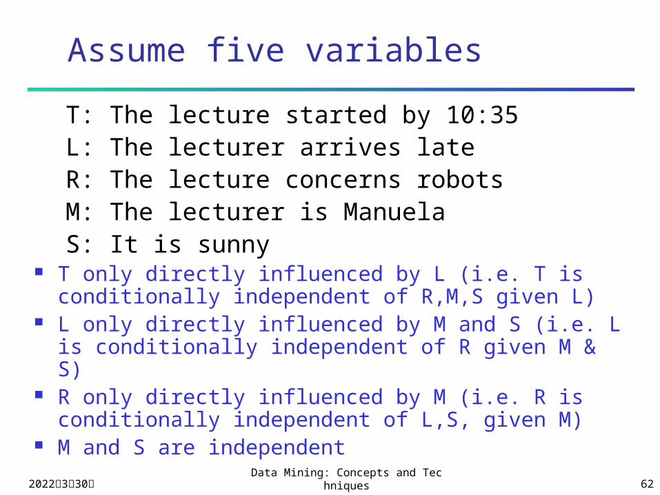
T: The lecture started by 10:35L: The lecturer arrives lateR: The lecture concerns robotsM: The lecturer is ManuelaS: It is sunny
T only directly influenced by L (i.e. T is conditionally independent of R,M,S given L)
L only directly influenced by M and S (i.e. L is conditionally independent of R given M & S)
R only directly influenced by M (i.e. R is conditionally independent of L,S, given M)
M and S are independent

2023年4月18日Data Mining: Concepts and Technique
s 63
Making a Bayes net
S M
R
L
T
Step One: add variables.• Just choose the variables you’d like to be included in the
net.
T: The lecture started by 10:35L: The lecturer arrives lateR: The lecture concerns robotsM: The lecturer is ManuelaS: It is sunny

2023年4月18日Data Mining: Concepts and Technique
s 64
Making a Bayes net
S M
R
L
T
Step Two: add links.• The link structure must be acyclic.• If node X is given parents Q1,Q2,..Qn you are promising
that any variable that’s a non-descendent of X is conditionally independent of X given {Q1,Q2,..Qn}
T: The lecture started by 10:35L: The lecturer arrives lateR: The lecture concerns robotsM: The lecturer is ManuelaS: It is sunny

2023年4月18日Data Mining: Concepts and Technique
s 65
Making a Bayes net
S M
R
L
T
P(s)=0.3P(M)=0.6
P(RM)=0.3P(R~M)=0.6
P(TL)=0.3P(T~L)=0.8
P(LM^S)=0.05P(LM^~S)=0.1P(L~M^S)=0.1P(L~M^~S)=0.2
Step Three: add a probability table for each node.• The table for node X must list P(X|Parent Values) for each
possible combination of parent values
T: The lecture started by 10:35L: The lecturer arrives lateR: The lecture concerns robotsM: The lecturer is ManuelaS: It is sunny

2023年4月18日Data Mining: Concepts and Technique
s 66
Computing with Bayes Net
P(T ^ ~R ^ L ^ ~M ^ S) =P(T ~R ^ L ^ ~M ^ S) * P(~R ^ L ^ ~M ^ S) = P(T L) * P(~R ^ L ^ ~M ^ S) =P(T L) * P(~R L ^ ~M ^ S) * P(L^~M^S) =P(T L) * P(~R ~M) * P(L^~M^S) =P(T L) * P(~R ~M) * P(L~M^S)*P(~M^S) =P(T L) * P(~R ~M) * P(L~M^S)*P(~M | S)*P(S) =P(T L) * P(~R ~M) * P(L~M^S)*P(~M)*P(S).
S M
RL
T
P(s)=0.3P(M)=0.6
P(RM)=0.3P(R~M)=0.6
P(TL)=0.3P(T~L)=0.8
P(LM^S)=0.05P(LM^~S)=0.1P(L~M^S)=0.1P(L~M^~S)=0.2

2023年4月18日Data Mining: Concepts and Technique
s 67
What we learned?
4. Data warehousing concept, schema
data cube & operations (rollup, …)
cube computation: multi-way array aggregation
iceberg cube
dynamic data cube
2023年4月18日Data Mining: Concepts and Technique
s 68
What is Data Warehouse?
Defined in many different ways, but not rigorously.
A decision support database that is maintained
separately from the organization’s operational database
Support information processing by providing a solid
platform of consolidated, historical data for analysis.
“A data warehouse is a subject-oriented, integrated, time-
variant, and nonvolatile collection of data in support of
management’s decision-making process.”—W. H. Inmon
Data warehousing:
The process of constructing and using data warehouses
2023年4月18日Data Mining: Concepts and Technique
s 69
Conceptual Modeling of Data Warehouses
Modeling data warehouses: dimensions & measures Star schema: A fact table in the middle connected
to a set of dimension tables Snowflake schema: A refinement of star schema
where some dimensional hierarchy is normalized
into a set of smaller dimension tables, forming a
shape similar to snowflake Fact constellations: Multiple fact tables share
dimension tables, viewed as a collection of stars,
therefore called galaxy schema or fact
constellation

2023年4月18日Data Mining: Concepts and Technique
s 70
A data cube
all
product quarter country
product, quarter product,country quarter, country
product, quarter, country
0-D(apex) cuboid
1-D cuboids
2-D cuboids
3-D(base) cuboid
2023年4月18日Data Mining: Concepts and Technique
s 71
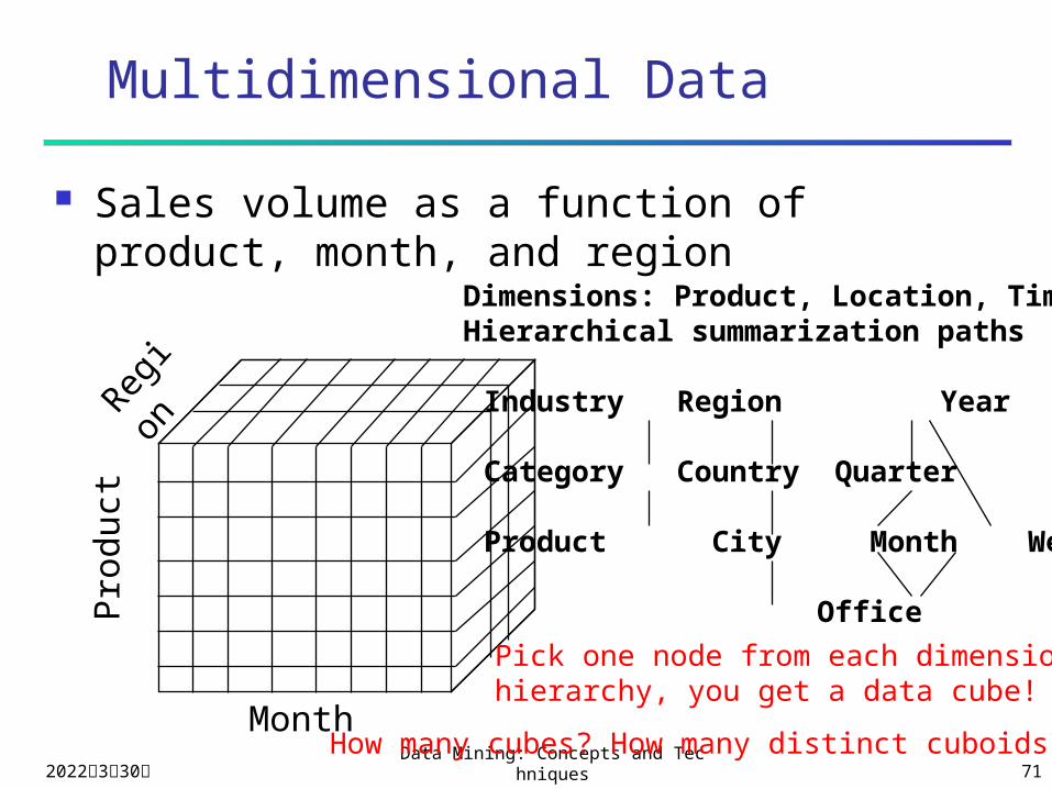
Multidimensional Data
Sales volume as a function of product, month, and region
Pro
duct
Regio
n
Month
Dimensions: Product, Location, TimeHierarchical summarization paths
Industry Region Year
Category Country Quarter
Product City Month Week
Office Day
Pick one node from each dimensionhierarchy, you get a data cube!
How many cubes? How many distinct cuboids?
2023年4月18日Data Mining: Concepts and Technique
s 72
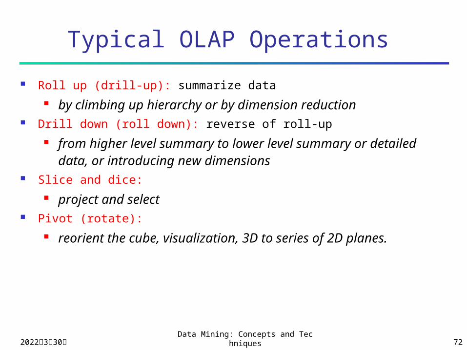
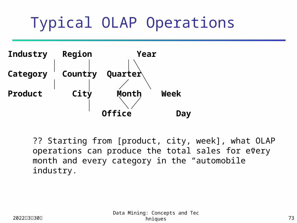
Typical OLAP Operations
Roll up (drill-up): summarize data by climbing up hierarchy or by dimension reduction
Drill down (roll down): reverse of roll-up from higher level summary to lower level summary or
detailed data, or introducing new dimensions Slice and dice:
project and select Pivot (rotate):
reorient the cube, visualization, 3D to series of 2D planes.
2023年4月18日Data Mining: Concepts and Technique
s 73
Typical OLAP Operations
Industry Region Year
Category Country Quarter
Product City Month Week
Office Day
?? Starting from [product, city, week], what OLAP operations can produce the total sales for every month and every category in the “automobile” industry.
2023年4月18日Data Mining: Concepts and Technique
s 74
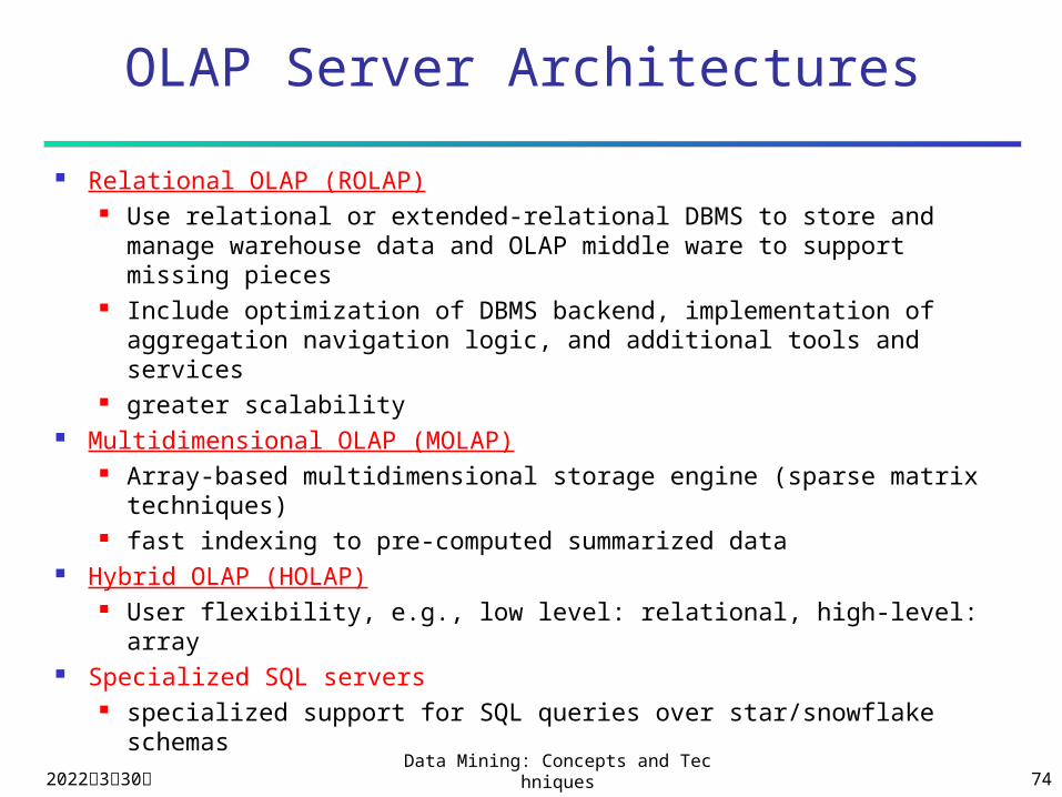
OLAP Server Architectures
Relational OLAP (ROLAP) Use relational or extended-relational DBMS to store and
manage warehouse data and OLAP middle ware to support missing pieces
Include optimization of DBMS backend, implementation of aggregation navigation logic, and additional tools and services
greater scalability Multidimensional OLAP (MOLAP)
Array-based multidimensional storage engine (sparse matrix techniques)
fast indexing to pre-computed summarized data Hybrid OLAP (HOLAP)
User flexibility, e.g., low level: relational, high-level: array Specialized SQL servers
specialized support for SQL queries over star/snowflake schemas
2023年4月18日Data Mining: Concepts and Technique
s 75
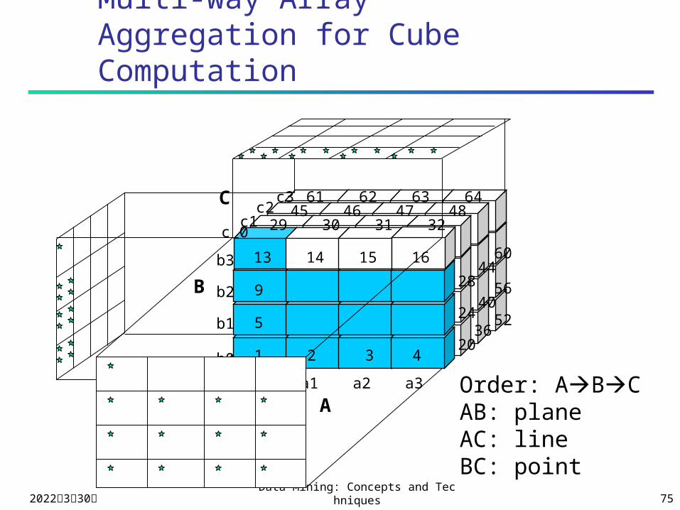
Multi-way Array Aggregation for Cube Computation
A
B
29 30 31 32
1 2 3 4
5
9
13 14 15 16
6463626148474645
a1a0
c3c2
c1c 0
b3
b2
b1
b0
a2 a3
C
4428 56
4024 52
3620
60
B
Order: ABCAB: planeAC: lineBC: point

2023年4月18日Data Mining: Concepts and Technique
s 76
Multi-Way Array Aggregation for Cube Computation (Cont.)
Let A: 40 values, B: 400 values, C: 4000 values. One chunk contains 10*100*1000 = 1,000,000
values. ABC needs how much memory?
AB plane: 40*400=16,000 AC line: 40*(4000/4) = 40,000 BC point: (400/4)*(4000/4) = 100,000 total: 156,000
CBA needs how much memory? CB plane: 4000*400=1,600,000 CA line: 4000*(40/4) = 40,000 BA point: (400/4)*(40/4) = 1000 total: 1,641,000 --- 10 times more!

2023年4月18日Data Mining: Concepts and Technique
s 77
Computing iceberg cube using BUC
BUC (Beyer & Ramakrishnan, SIGMOD’99) Bottom-up vs. top-down?—depending on how you view it! Apriori property:
Aggregate the data, then move to the next level If minsup is not met, stop!
2023年4月18日Data Mining: Concepts and Technique
s 78
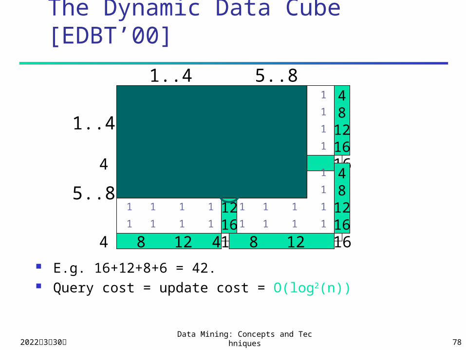
The Dynamic Data Cube [EDBT’00]
E.g. 16+12+8+6 = 42. Query cost = update cost = O(log2(n))
1..4 5..8
1..4
5..8
4 8 12 16
4812161111
1111
1111
11114 8 12 16
4812161111
1111
1111
1111
4 8 12 16
4812161111
1111
1111
1111
4 8 12 16
4812161111
1111
1111
1111
2023年4月18日Data Mining: Concepts and Technique
s 79
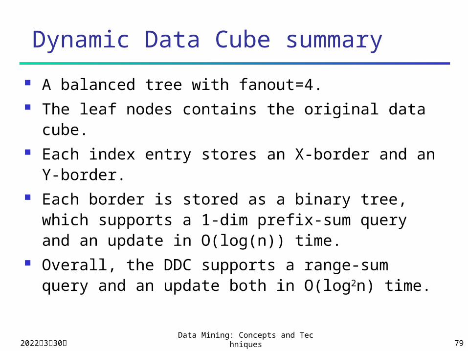
Dynamic Data Cube summary
A balanced tree with fanout=4. The leaf nodes contains the original data cube. Each index entry stores an X-border and an Y-
border. Each border is stored as a binary tree, which
supports a 1-dim prefix-sum query and an update in O(log(n)) time.
Overall, the DDC supports a range-sum query and an update both in O(log2n) time.
2023年4月18日Data Mining: Concepts and Technique
s 80
5. Additional lattice (of itemsets, g-itemsets, rules, cuboids)
distance-based indexing

2023年4月18日Data Mining: Concepts and Technique
s 81
Problem Statement
Given a set S of objects and a metric distance function d(). The similarity search problem is defined as: for an arbitrary object q and a threshold , find{ o | oS d(o, q)< }
Solution without index: for every oS, compute d(q,o). Not efficient!
2023年4月18日Data Mining: Concepts and Technique
s 82
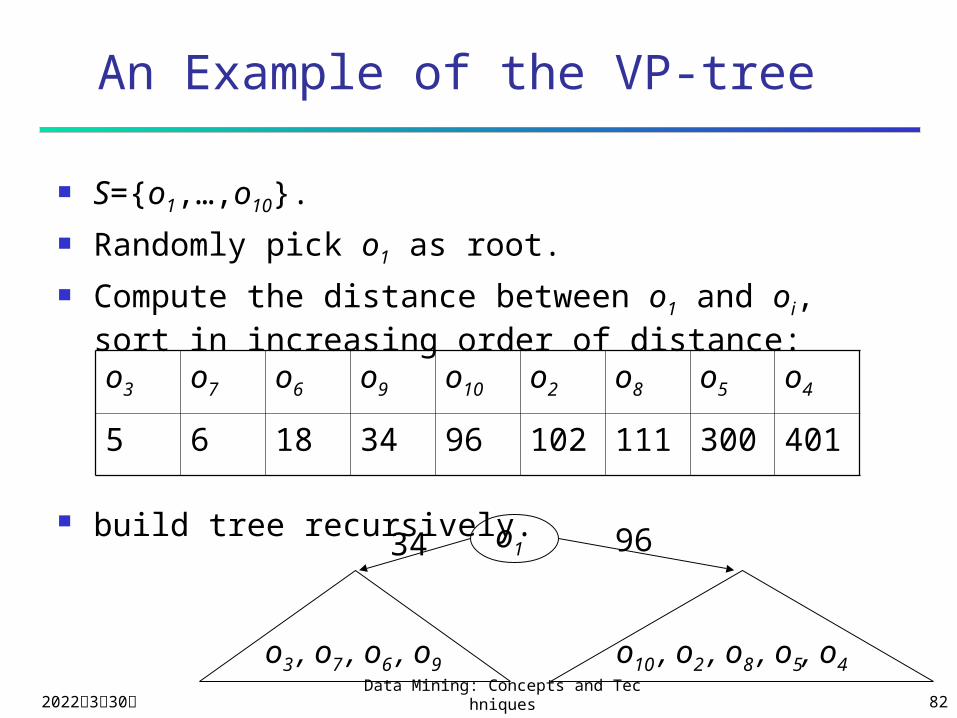
An Example of the VP-tree
S={o1,…,o10}. Randomly pick o1 as root. Compute the distance between o1 and oi, sort in
increasing order of distance:
build tree recursively.
o3 o7 o6 o9 o10 o2 o8 o5 o4
5 6 18 34 96 102 111 300 401
o1
o3 , o7 , o6 , o9 o10 , o2 , o8 , o5, o4
34 96
2023年4月18日Data Mining: Concepts and Technique
s 83
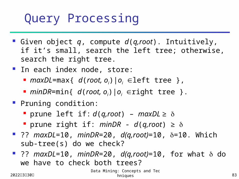
Query Processing
Given object q, compute d(q,root). Intuitively, if it’s small, search the left tree; otherwise, search the right tree.
In each index node, store: maxDL=max{ d(root, oi)|oi left tree }, minDR=min{ d(root, oi)|oi right tree }.
Pruning condition: prune left if: d(q,root) – maxDL ≥ prune right if: minDR - d(q,root) ≥
?? maxDL=10, minDR=20, d(q,root)=10, =10. Which sub-tree(s) do we check?
?? maxDL=10, minDR=20, d(q,root)=10, for what do we have to check both trees?
2023年4月18日Data Mining: Concepts and Technique
s 84
Summary
1. Frequent pattern & association
2. Clustering
3. Classification
4. Data warehousing
5. Additional