Embed Size (px)
Citation preview
2015-2016 40
Prof. Dr. Mustafa B. Dawood Dr. Bilal Ismaeel Al-Shraify
Chapter Two
Yield line
2015-2016 41
Prof. Dr. Mustafa B. Dawood Dr. Bilal Ismaeel Al-Shraify
Yield line analysis for slabs
Most concrete slabs are designed for moments found by the methods based essentially upon elastic theory. On the other hand, reinforcement for slabs is calculated by strength methods. That account for the actual inelastic behavior of member at the factored load stage. A corresponding contradiction exists in the process by which beams and frames are analyzed and designed, and the concept of limit, or plastic analysis of reinforced concrete was introduced.
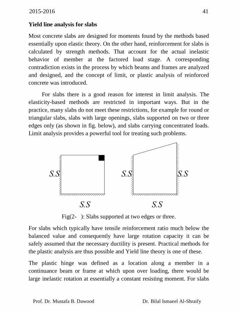
For slabs there is a good reason for interest in limit analysis. The elasticity-based methods are restricted in important ways. But in the practice, many slabs do not meet these restrictions, for example for round or triangular slabs, slabs with large openings, slabs supported on two or three edges only (as shown in fig. below), and slabs carrying concentrated loads. Limit analysis provides a powerful tool for treating such problems.
Fig(2- ): Slabs supported at two edges or three.
For slabs which typically have tensile reinforcement ratio much below the balanced value and consequently have large rotation capacity it can be safely assumed that the necessary ductility is present. Practical methods for the plastic analysis are thus possible and Yield line theory is one of these.
The plastic hinge was defined as a location along a member in a continuance beam or frame at which upon over loading, there would be large inelastic rotation at essentially a constant resisting moment. For slabs
2015-2016 42
Prof. Dr. Mustafa B. Dawood Dr. Bilal Ismaeel Al-Shraify
the corresponding mechanism is the yield line. The yield line serves as an axis of rotation for the slab segment.
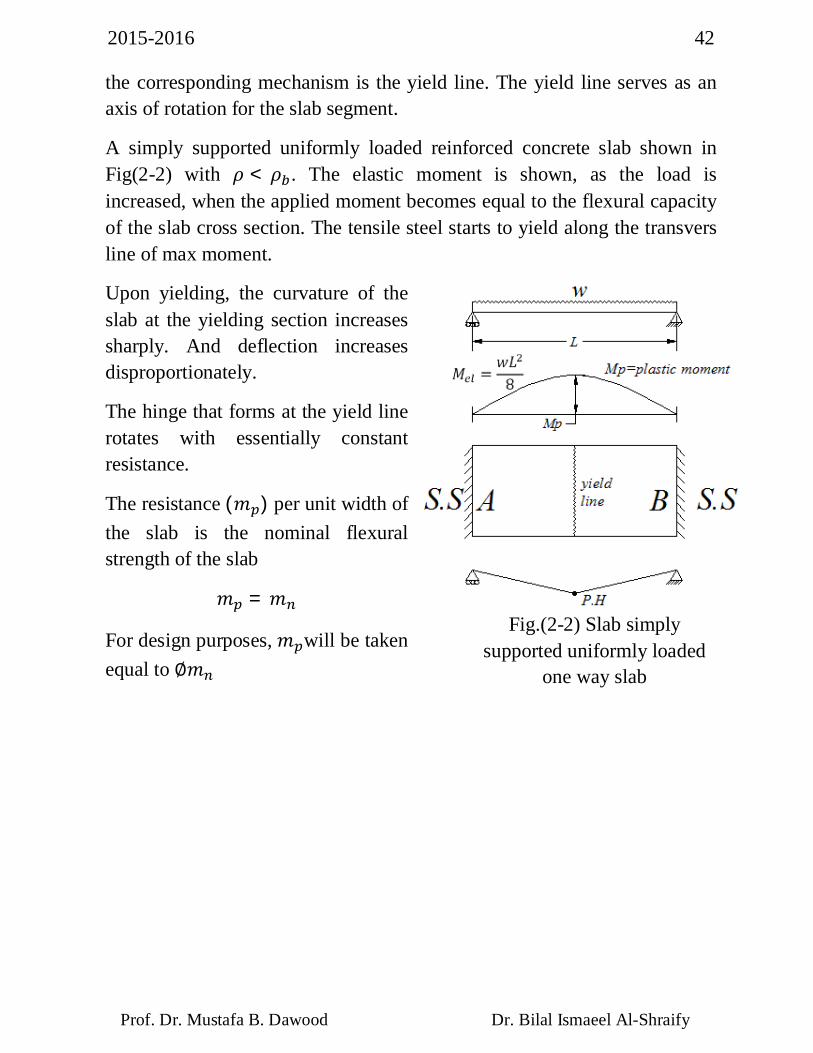
A simply supported uniformly loaded reinforced concrete slab shown in Fig(2-2) with 휌 < 휌 . The elastic moment is shown, as the load is increased, when the applied moment becomes equal to the flexural capacity of the slab cross section. The tensile steel starts to yield along the transvers line of max moment.
Upon yielding, the curvature of the slab at the yielding section increases sharply. And deflection increases disproportionately.
The hinge that forms at the yield line rotates with essentially constant resistance.
The resistance (푚 ) per unit width of the slab is the nominal flexural strength of the slab
푚 = 푚
For design purposes, 푚 will be taken equal to ∅푚
Fig.(2-2) Slab simply supported uniformly loaded
one way slab
2015-2016 43
Prof. Dr. Mustafa B. Dawood Dr. Bilal Ismaeel Al-Shraify
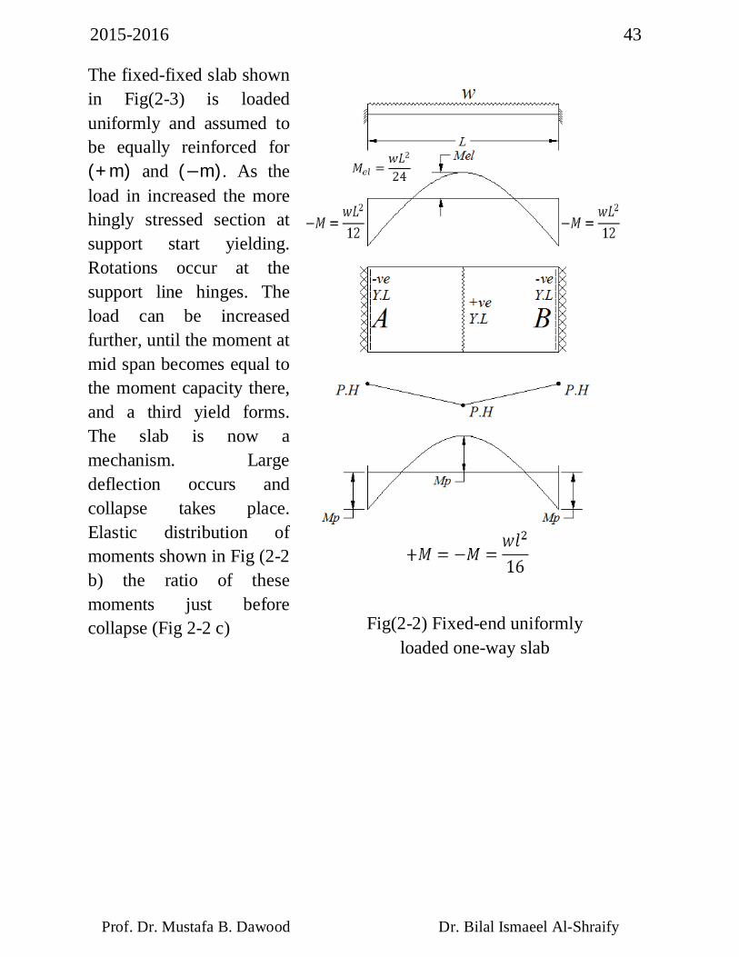
The fixed-fixed slab shown in Fig(2-3) is loaded uniformly and assumed to be equally reinforced for (+m) and (−m). As the load in increased the more hingly stressed section at support start yielding. Rotations occur at the support line hinges. The load can be increased further, until the moment at mid span becomes equal to the moment capacity there, and a third yield forms. The slab is now a mechanism. Large deflection occurs and collapse takes place. Elastic distribution of moments shown in Fig (2-2 b) the ratio of these moments just before collapse (Fig 2-2 c)
Fig(2-2) Fixed-end uniformly loaded one-way slab
2015-2016 44
Prof. Dr. Mustafa B. Dawood Dr. Bilal Ismaeel Al-Shraify
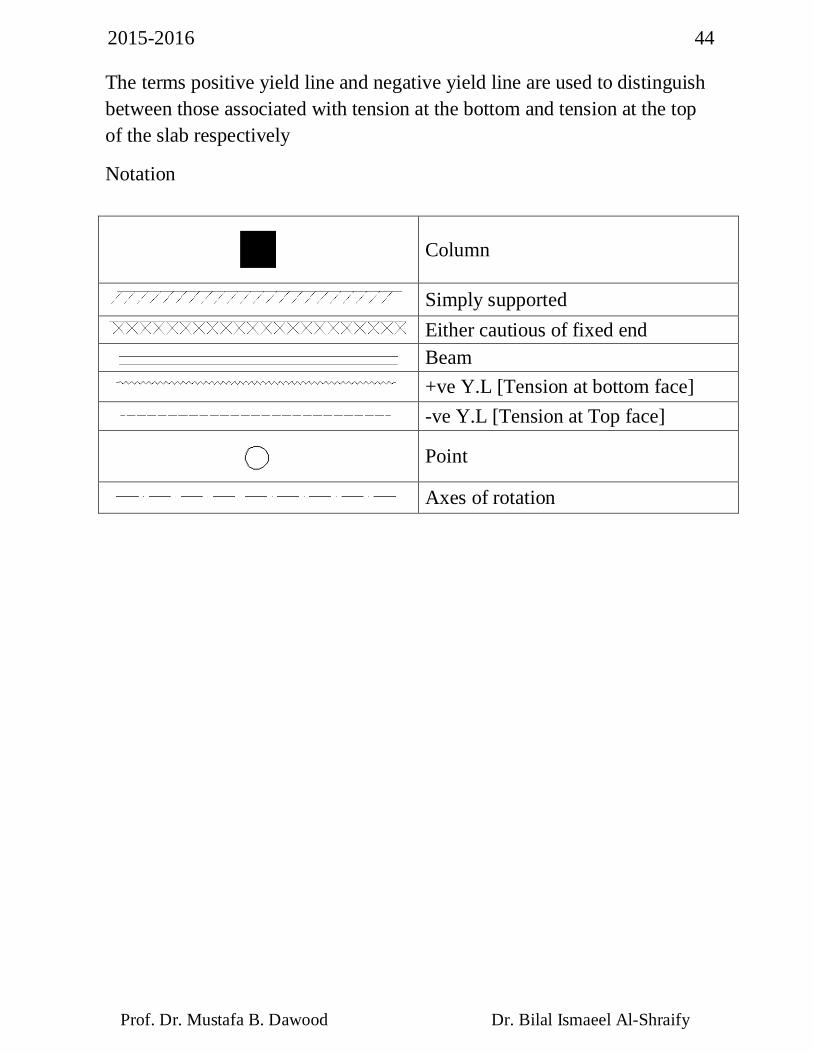
The terms positive yield line and negative yield line are used to distinguish between those associated with tension at the bottom and tension at the top of the slab respectively
Notation
Column
Simply supported
Either cautious of fixed end Beam
+ve Y.L [Tension at bottom face]
-ve Y.L [Tension at Top face]
Point
Axes of rotation
2015-2016 45
Prof. Dr. Mustafa B. Dawood Dr. Bilal Ismaeel Al-Shraify
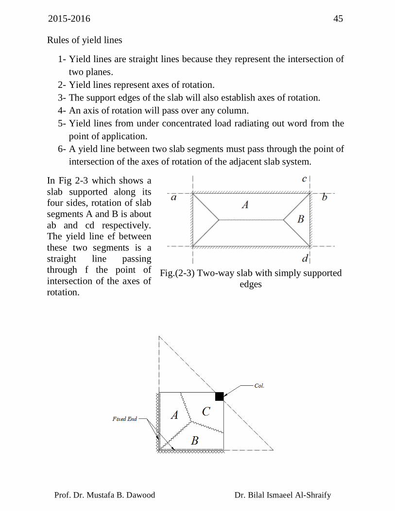
Rules of yield lines
1- Yield lines are straight lines because they represent the intersection of two planes.
2- Yield lines represent axes of rotation. 3- The support edges of the slab will also establish axes of rotation. 4- An axis of rotation will pass over any column. 5- Yield lines from under concentrated load radiating out word from the
point of application. 6- A yield line between two slab segments must pass through the point of
intersection of the axes of rotation of the adjacent slab system.
In Fig 2-3 which shows a slab supported along its four sides, rotation of slab segments A and B is about ab and cd respectively. The yield line ef between these two segments is a straight line passing through f the point of intersection of the axes of rotation.
Fig.(2-3) Two-way slab with simply supported
edges
2015-2016 46
Prof. Dr. Mustafa B. Dawood Dr. Bilal Ismaeel Al-Shraify
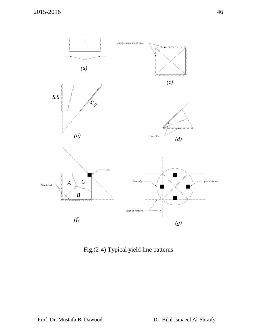
four ColumnFree edge
Axes of rotation
Fixed End
Col.
B
A C
Fixed End
S.SS.S
Simply supported all sides
(a)
(c)
(b) (d)
(f) (g)
Fig.(2-4) Typical yield line patterns
2015-2016 47
Prof. Dr. Mustafa B. Dawood Dr. Bilal Ismaeel Al-Shraify
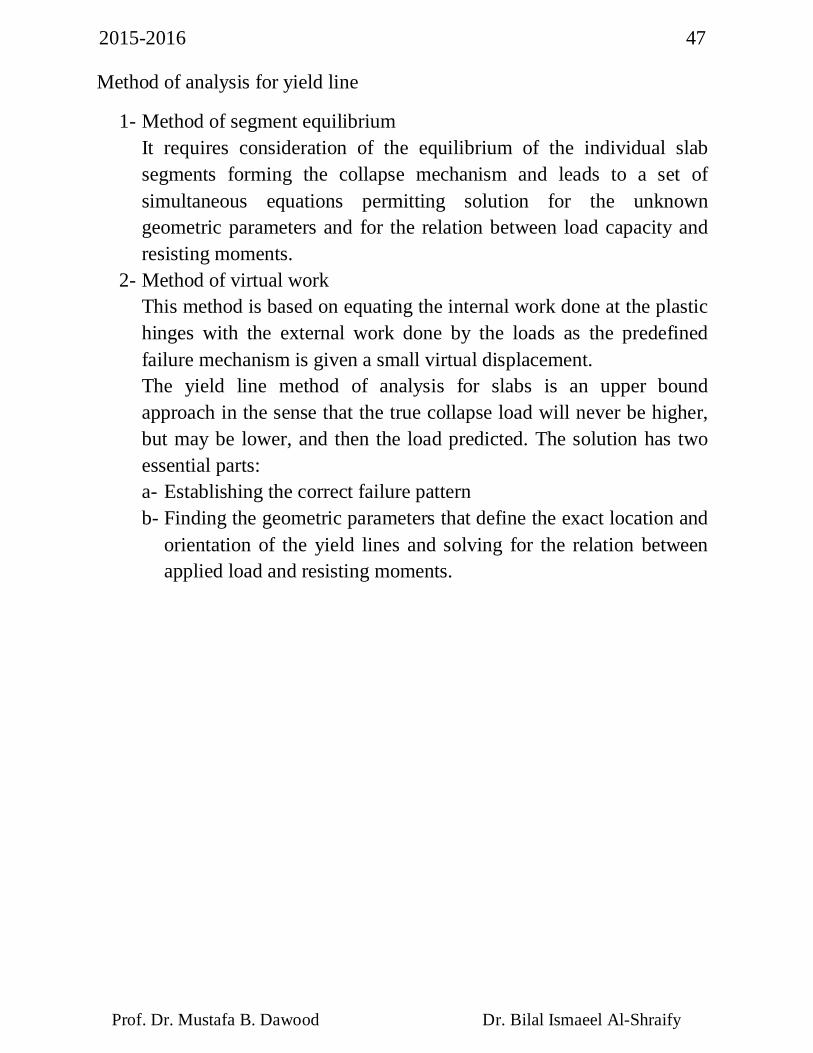
Method of analysis for yield line
1- Method of segment equilibrium It requires consideration of the equilibrium of the individual slab segments forming the collapse mechanism and leads to a set of simultaneous equations permitting solution for the unknown geometric parameters and for the relation between load capacity and resisting moments.
2- Method of virtual work This method is based on equating the internal work done at the plastic hinges with the external work done by the loads as the predefined failure mechanism is given a small virtual displacement. The yield line method of analysis for slabs is an upper bound approach in the sense that the true collapse load will never be higher, but may be lower, and then the load predicted. The solution has two essential parts: a- Establishing the correct failure pattern b- Finding the geometric parameters that define the exact location and
orientation of the yield lines and solving for the relation between applied load and resisting moments.
2015-2016 48
Prof. Dr. Mustafa B. Dawood Dr. Bilal Ismaeel Al-Shraify
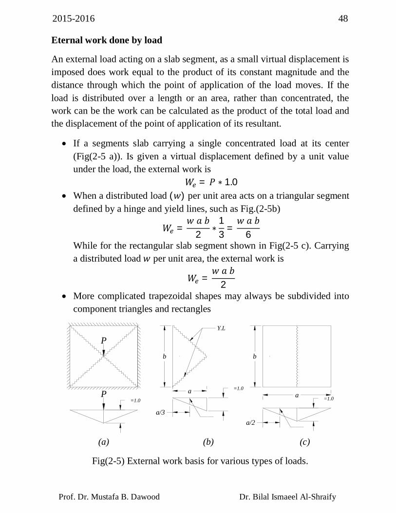
Eternal work done by load
An external load acting on a slab segment, as a small virtual displacement is imposed does work equal to the product of its constant magnitude and the distance through which the point of application of the load moves. If the load is distributed over a length or an area, rather than concentrated, the work can be the work can be calculated as the product of the total load and the displacement of the point of application of its resultant.
If a segments slab carrying a single concentrated load at its center (Fig(2-5 a)). Is given a virtual displacement defined by a unit value under the load, the external work is
푊 = 푃 ∗ 1.0 When a distributed load (푤) per unit area acts on a triangular segment
defined by a hinge and yield lines, such as Fig.(2-5b)
푊 =푤 푎 푏
2 ∗13 =
푤 푎 푏6
While for the rectangular slab segment shown in Fig(2-5 c). Carrying a distributed load 푤 per unit area, the external work is
푊 =푤 푎 푏
2
More complicated trapezoidal shapes may always be subdivided into component triangles and rectangles
P
a
b
Y.L
a/3
=1.0
=1.0P a
b
a/2
=1.0
(a) (b) (c)
Fig(2-5) External work basis for various types of loads.
2015-2016 49
Prof. Dr. Mustafa B. Dawood Dr. Bilal Ismaeel Al-Shraify
Internal work done by resisting moments:
The internal work done during the assigned virtual displacement is found by summing the production of yield moment (푚) per unit length of hinge times the plastic rotation (휃) at the respective yield lines. If the resisting moment(푚) is constant along a yield line of length (퐿) and if a rotation (휃) is experienced, the internal work is :
푤 = 푚퐿∅ 퐿 = 퐿푒푛푔푡ℎ 표푓 푦푖푒푙푑 푙푖푛푒
For the entire system, the total internal work done is the sum of the contributions from all yield lines.
2015-2016 50
Prof. Dr. Mustafa B. Dawood Dr. Bilal Ismaeel Al-Shraify
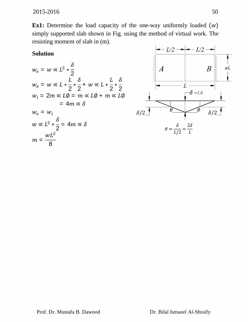
Ex1: Determine the load capacity of the one-way uniformly loaded (푤) simply supported slab shown in Fig. using the method of virtual work. The resisting moment of slab in (m).
Solution
푤 = 푤 ∝ 퐿 ∗훿2
푤 = 푤 ∝ 퐿 ∗퐿2∗훿2
+ 푤 ∝ 퐿 ∗퐿2∗훿2
푤 = 2푚 ∝ 퐿∅ = 푚 ∝ 퐿∅ + 푚 ∝ 퐿∅= 4푚 ∝ 훿
푤 = 푤
푤 ∝ 퐿 ∗훿2
= 4푚 ∝ 훿
푚 =푤퐿
8
2015-2016 51
Prof. Dr. Mustafa B. Dawood Dr. Bilal Ismaeel Al-Shraify
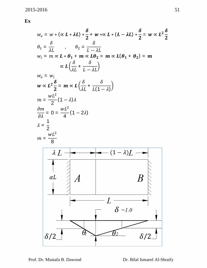
Ex
푤 = 푤 ∗ (∝ 푳 ∗ 흀푳) ∗휹ퟐ + 풘 ∗∝ 푳 ∗ (푳 − 흀푳) ∗
휹ퟐ = 풘 ∝ 푳ퟐ
휹ퟐ
휃 =훿휆퐿 , 휃 =
훿퐿 − 휆퐿
푤 = 푚 ∝ 푳 ∗ 휽ퟏ +풎 ∝ 푳휽ퟐ = 풎 ∝ 푳(휽ퟏ + 휽ퟐ) = 풎
∝ 푳훿휆퐿 +
훿퐿 − 휆퐿
푤 = 푤
풘 ∝ 푳ퟐ휹ퟐ
= 풎 ∝ 푳훿휆퐿
+훿
퐿(1− 휆)
푚 =푤퐿
2(1− 휆)휆
휕푚휕휆 = 0 =
푤퐿4
(1 − 2휆)
휆 =12
푚 =푤퐿
8
2015-2016 52
Prof. Dr. Mustafa B. Dawood Dr. Bilal Ismaeel Al-Shraify
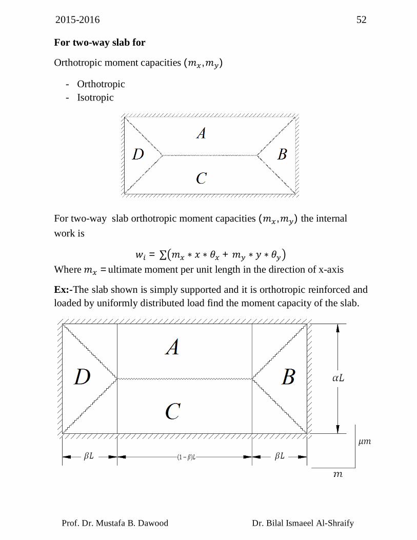
For two-way slab for
Orthotropic moment capacities (푚 ,푚 )
- Orthotropic - Isotropic
For two-way slab orthotropic moment capacities (푚 ,푚 ) the internal work is
푤 = ∑ 푚 ∗ 푥 ∗ 휃 +푚 ∗ 푦 ∗ 휃 Where 푚 =ultimate moment per unit length in the direction of x-axis
Ex:-The slab shown is simply supported and it is orthotropic reinforced and loaded by uniformly distributed load find the moment capacity of the slab.
2015-2016 53
Prof. Dr. Mustafa B. Dawood Dr. Bilal Ismaeel Al-Shraify
Solution
∑푀휃 = ∑ 푀 ∗ 휃 + 푀 ∗ 휃 = 휇푚 ∗ 퐿 ∗1훽퐿
∑푀휃 = ∑ 푀 휃 + 푀 휃 = 푚 ∗ 퐿 ∗2훼퐿
∑푀휃 , , , =
∑푤훿 =푤훼퐿
2 ∗ (1− 2훽) ∗ 퐿 ∗12 +
푤훼퐿2 ∗ (1 − 2훽) ∗ 퐿 ∗
12
+ 푤훽퐿 ∗훼퐿2 ∗
13 ∗ 4 + 푤 ∗
훼퐿훽퐿2 ∗
13 ∗ 2
or ∑푤훿 = 푤훼퐿(1− 2훽)퐿 ∗12
+ 푤훼퐿 ∗ 훽퐿 ∗13
∗ 퐿
= 푤훼퐿23훽퐿 +
1 − 2훽2
… … … … … . . (퐼퐼)
∑푀휃 = ∑푤훿
푚 =1
12 ∗ 푤 ∗ 훼 퐿 ∗3훽 − 2훽2훽 + 휇훼 →
휕푚휕훽 = 0
3훽 − 2훽2훽 + 휇훼 =
3− 4훽2
4훽 + 4휇훼 훽 − 3휇훼 = 0
훽 =12 3휇훼 + 휇 훼 − 휇훼
∴ 푚 =1
24푤훼 퐿 3 + 휇훼 − 훼 휇
2015-2016 54
Prof. Dr. Mustafa B. Dawood Dr. Bilal Ismaeel Al-Shraify
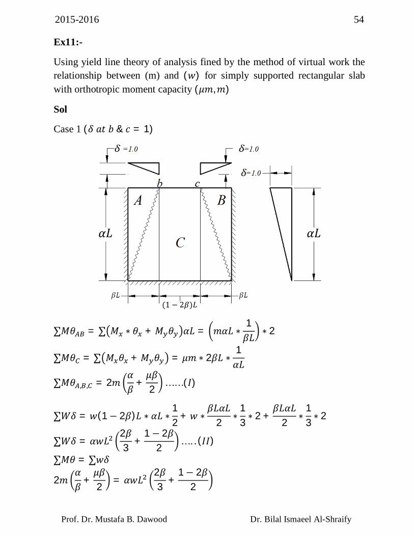
Ex11:-
Using yield line theory of analysis fined by the method of virtual work the relationship between (m) and (푤) for simply supported rectangular slab with orthotropic moment capacity (휇푚,푚)
Sol
Case 1 (훿 푎푡 푏 & 푐 = 1)
∑푀휃 = ∑ 푀 ∗ 휃 + 푀 휃 훼퐿 = 푚훼퐿 ∗1훽퐿 ∗ 2
∑푀휃 = ∑ 푀 휃 +푀 휃 = 휇푚 ∗ 2훽퐿 ∗1훼퐿
∑푀휃 , , = 2푚훼훽 +
휇훽2 … … (퐼)
∑푊훿 = 푤(1− 2훽)퐿 ∗ 훼퐿 ∗12 + 푤 ∗
훽퐿훼퐿2 ∗
13 ∗ 2 +
훽퐿훼퐿2 ∗
13 ∗ 2
∑푊훿 = 훼푤퐿2훽3 +
1 − 2훽2 … . . (퐼퐼)
∑푀휃 = ∑푤훿
2푚훼훽 +
휇훽2 = 훼푤퐿
2훽3 +
1− 2훽2
2015-2016 55
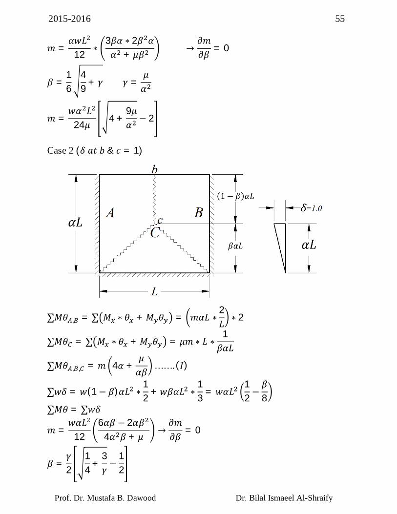
Prof. Dr. Mustafa B. Dawood Dr. Bilal Ismaeel Al-Shraify
푚 =훼푤퐿
12 ∗3훽훼 ∗ 2훽 훼훼 + 휇훽 →
휕푚휕훽 = 0
훽 =16
49 + 훾 훾 =
휇훼
푚 =푤훼 퐿
24휇 4 +9휇훼 − 2
Case 2 (훿 푎푡 푏 & 푐 = 1)
∑푀휃 , = ∑ 푀 ∗ 휃 +푀 휃 = 푚훼퐿 ∗2퐿
∗ 2
∑푀휃 = ∑ 푀 ∗ 휃 +푀 휃 = 휇푚 ∗ 퐿 ∗1훽훼퐿
∑푀휃 , , = 푚 4훼 +휇훼훽 … … . (퐼)
∑푤훿 = 푤(1− 훽)훼퐿 ∗12 +푤훽훼퐿 ∗
13 = 푤훼퐿
12 −
훽8
∑푀휃 = ∑푤훿
푚 =푤훼퐿
126훼훽 − 2훼훽
4훼 훽 + 휇→휕푚휕훽
= 0
훽 =훾2
14 +
3훾 −
12
2015-2016 56
Prof. Dr. Mustafa B. Dawood Dr. Bilal Ismaeel Al-Shraify
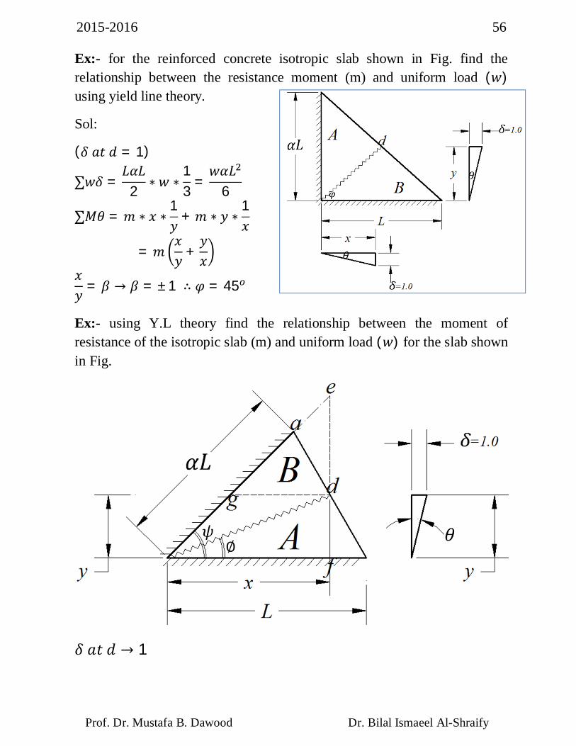
Ex:- for the reinforced concrete isotropic slab shown in Fig. find the relationship between the resistance moment (m) and uniform load (푤) using yield line theory.
Sol:
(훿 푎푡 푑 = 1)
∑푤훿 =퐿훼퐿
2∗ 푤 ∗
13
=푤훼퐿
6
∑푀휃 = 푚 ∗ 푥 ∗1푦
+푚 ∗ 푦 ∗1푥
= 푚푥푦 +
푦푥
푥푦 = 훽 → 훽 = ±1 ∴ 휑 = 45
Ex:- using Y.L theory find the relationship between the moment of resistance of the isotropic slab (m) and uniform load (푤) for the slab shown in Fig.
훿 푎푡 푑 → 1
2015-2016 57
Prof. Dr. Mustafa B. Dawood Dr. Bilal Ismaeel Al-Shraify
Solution
∑푀휃 = ∑ 푀푥 ∗ 휃푥 + 푀푦휃푦 = 푚 ∗ 푥 ∗1푦
= 푚 ∗푥푦
= 푚 cot(휃)
∑푀휃 = ∑ 푀푥 ∗ 휃푥 + 푀푦휃푦 = 푚 ∗ 푥 ∗1푑푒
+ 푚 ∗ 푦 ∗1푑푔
푑푒 = 푒푓 − 푦 = 푥 tan(휓)− 푦 = 푥 tan(휓) − 푥 tan(휃) 푑푔 = 푥 − 푦 cot(휓) = 푦 cot(휃)− 푦 cot(휓) = 푦(cot(휃) − cot(휓))
∑푀휃 = 푚1
tan(휓) − tan(휃) +1
cot(휃) − cot(휓)
= 푚1 + tan(휓) cot(휃)tan(휓) − tan(휃) = 푚[cot(휓 − 휃)]
∑푀휃 , = 푚(cot(휃) + cot(휓 − 휃))
∑푤훿 =13 ∗ 푤
12 ∗ 훼퐿 ∗ 퐿 ∗ sin(휓) =
16 ∗ 푤 ∗ 훼 ∗ 퐿 sin(휓)
∑푀휃 = ∑푤훿
푚 =푤훼 ∗ 퐿 ∗ sin(휓)
6[cot(휓 − 휃) + cot(휃)] =16푤 ∗ 훼 ∗ 퐿 ∗ sin(휃) sin(휓 − 휃)
휕푚휕휃 = 0
cos(휃) ∗ sin(휓 − 휃) = sin(휃) ∗ cos( 휓 − 휃) tan(휃) = tan(휓 − 휃)
∴ 휃 =12휓
푚 =16 ∗ 푤 ∗ 훼 ∗ 퐿 ∗ sin
휓2
2015-2016 58
Prof. Dr. Mustafa B. Dawood Dr. Bilal Ismaeel Al-Shraify
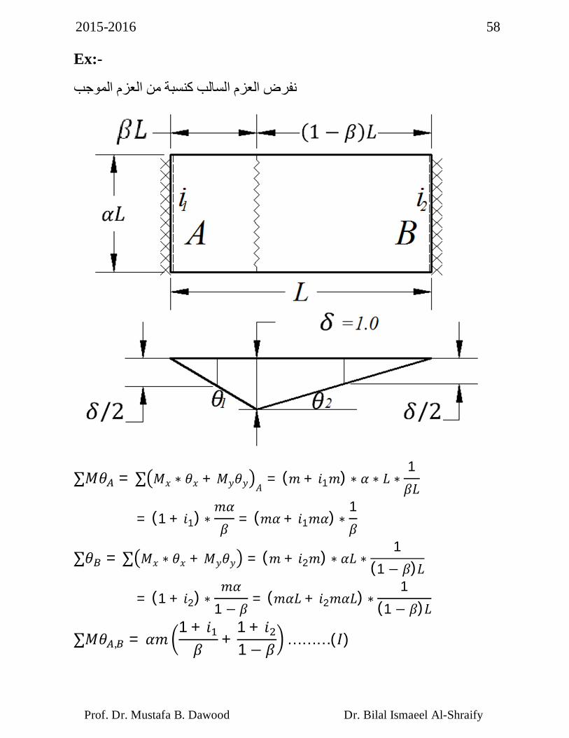
Ex:-
نفرض العزم السالب كنسبة من العزم الموجب
∑푀휃 = ∑ 푀푥 ∗ 휃푥 + 푀푦휃푦 퐴= (푚 + 푖1푚) ∗ 훼 ∗ 퐿 ∗
1훽퐿
= (1 + 푖1) ∗푚훼훽
= (푚훼 + 푖1푚훼) ∗1훽
∑휃 = ∑ 푀푥 ∗ 휃푥 + 푀푦휃푦 = (푚 + 푖2푚) ∗ 훼퐿 ∗1
(1 − 훽)퐿
= (1 + 푖2) ∗푚훼
1 − 훽= (푚훼퐿 + 푖2푚훼퐿) ∗
1(1 − 훽)퐿
∑푀휃 , = 훼푚1 + 푖훽 +
1 + 푖1 − 훽 … … … (퐼)
2015-2016 59
Prof. Dr. Mustafa B. Dawood Dr. Bilal Ismaeel Al-Shraify
∑푤훿 =12 ∗ 푤 ∗ 훼 ∗ 퐿
∑푀휃 = ∑푤훿 푤 ∗ 훼 ∗ 퐿
2 = 훼푚1 + 푖훽 +
1 + 푖1 − 훽
퐼퐹 푖 = 푖
푚 =푤퐿
4 ∗ (훽 − 훽 )
휕푚휕훽 = 0 → 훽 =
12
∴ 푚 =푤퐿16
2015-2016 60
Prof. Dr. Mustafa B. Dawood Dr. Bilal Ismaeel Al-Shraify
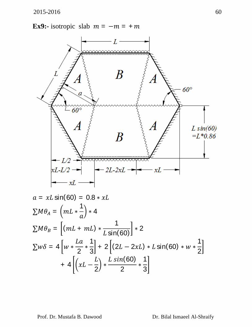
Ex9:- isotropic slab 푚 = −푚 = +푚
푎 = 푥퐿 sin(60) = 0.8 ∗ 푥퐿
∑푀휃 = 푚퐿 ∗1푎 ∗ 4
∑푀휃 = (푚퐿 + 푚퐿) ∗1
퐿 sin(60) ∗ 2
∑푤훿 = 4 푤 ∗퐿푎2 ∗
13 + 2 (2퐿 − 2푥퐿) ∗ 퐿 sin(60) ∗ 푤 ∗
12
+ 4 푥퐿 −퐿2 ∗
퐿 푠푖푛(60)2 ∗
13
2015-2016 61
Prof. Dr. Mustafa B. Dawood Dr. Bilal Ismaeel Al-Shraify
∑푤훿 = 4퐿 ∗ 퐿 sin(60)
2 ∗13 ∗ 푤
+ 2[(퐿 sin(60) ∗ 푥퐿 sin(60))푤]
+ 4푥퐿 sin(60) − ( )
6 ∗ 푤
∑푀휃 =4푚
sin(60)1 + 푥푥
∑푀휃 = ∑푤훿 퐿 sin(60)
3 ∗ 푤 ∗ (5 − 2푥) =4푚
sin(60)1 + 푥푥
푤 =16푚(1 + 푥)퐿 (5푥 − 2푥 )
휕푤휕푥 = 0 → 푥 = 0.87
∴ 푤 = 10.54 푚/퐿
2015-2016 62
Prof. Dr. Mustafa B. Dawood Dr. Bilal Ismaeel Al-Shraify
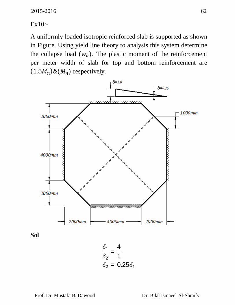
Ex10:-
A uniformly loaded isotropic reinforced slab is supported as shown in Figure. Using yield line theory to analysis this system determine the collapse load (푤 ). The plastic moment of the reinforcement per meter width of slab for top and bottom reinforcement are (1.5푀 )&(푀 ) respectively.
Sol
훿훿 =
41
훿 = 0.25훿
2015-2016 63
Prof. Dr. Mustafa B. Dawood Dr. Bilal Ismaeel Al-Shraify
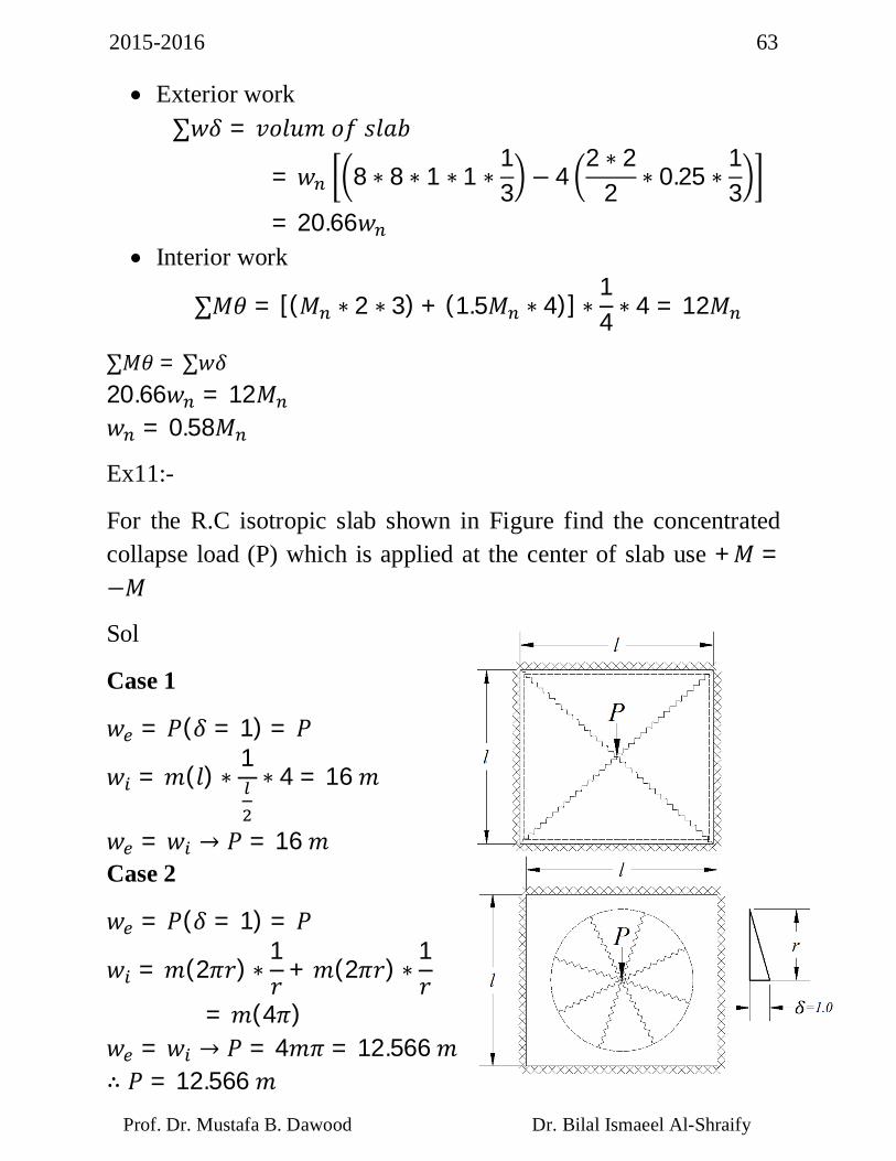
Exterior work ∑푤훿 = 푣표푙푢푚 표푓 푠푙푎푏
= 푤 8 ∗ 8 ∗ 1 ∗ 1 ∗13 − 4
2 ∗ 22 ∗ 0.25 ∗
13
= 20.66푤 Interior work
∑푀휃 = [(푀 ∗ 2 ∗ 3) + (1.5푀 ∗ 4)] ∗14 ∗ 4 = 12푀
∑푀휃 = ∑푤훿 20.66푤 = 12푀 푤 = 0.58푀
Ex11:-
For the R.C isotropic slab shown in Figure find the concentrated collapse load (P) which is applied at the center of slab use +푀 =−푀
Sol
Case 1
푤 = 푃(훿 = 1) = 푃
푤 = 푚(푙) ∗1∗ 4 = 16 푚
푤 = 푤 → 푃 = 16 푚 Case 2
푤 = 푃(훿 = 1) = 푃
푤 = 푚(2휋푟) ∗1푟 + 푚(2휋푟) ∗
1푟
= 푚(4휋) 푤 = 푤 → 푃 = 4푚휋 = 12.566 푚 ∴ 푃 = 12.566 푚
2015-2016 64
Prof. Dr. Mustafa B. Dawood Dr. Bilal Ismaeel Al-Shraify
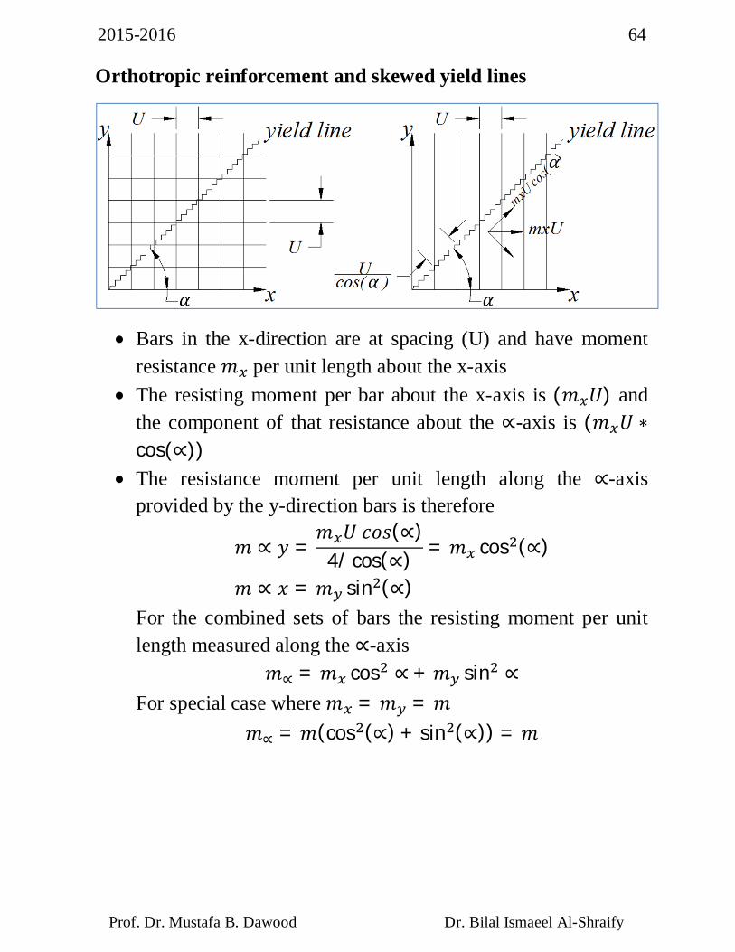
Orthotropic reinforcement and skewed yield lines
Bars in the x-direction are at spacing (U) and have moment resistance 푚 per unit length about the x-axis
The resisting moment per bar about the x-axis is (푚 푈) and the component of that resistance about the ∝-axis is (푚 푈 ∗cos (∝))
The resistance moment per unit length along the ∝-axis provided by the y-direction bars is therefore
푚 ∝ 푦 =푚 푈 푐표푠(∝)
4/ cos(∝) = 푚 cos (∝)
푚 ∝ 푥 = 푚 sin (∝) For the combined sets of bars the resisting moment per unit length measured along the ∝-axis
푚∝ = 푚 cos ∝ + 푚 sin ∝ For special case where 푚 = 푚 = 푚
푚∝ = 푚(cos (∝) + sin (∝)) = 푚
2015-2016 65
Prof. Dr. Mustafa B. Dawood Dr. Bilal Ismaeel Al-Shraify
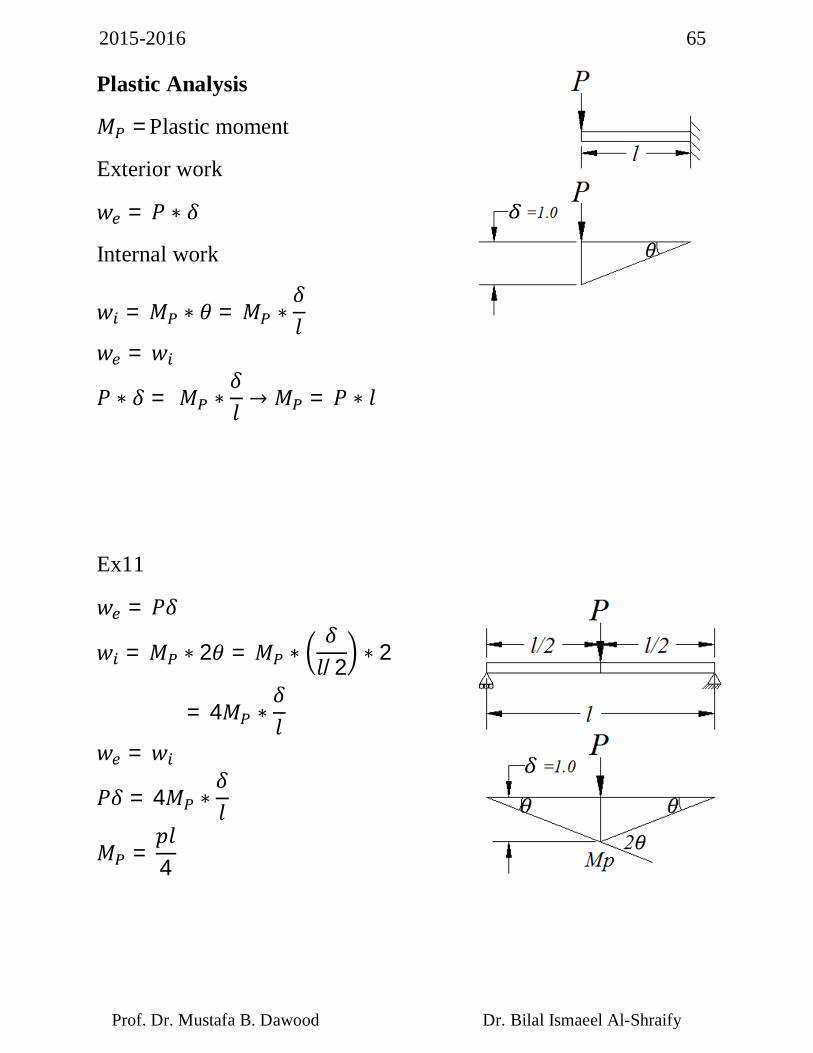
Plastic Analysis
푀 =Plastic moment
Exterior work
푤 = 푃 ∗ 훿
Internal work
푤 = 푀 ∗ 휃 = 푀 ∗훿푙
푤 = 푤
푃 ∗ 훿 = 푀 ∗훿푙 → 푀 = 푃 ∗ 푙
Ex11
푤 = 푃훿
푤 = 푀 ∗ 2휃 = 푀 ∗훿푙/2 ∗ 2
= 4푀 ∗훿푙
푤 = 푤
푃훿 = 4푀 ∗훿푙
푀 =푝푙4
2015-2016 66
Prof. Dr. Mustafa B. Dawood Dr. Bilal Ismaeel Al-Shraify
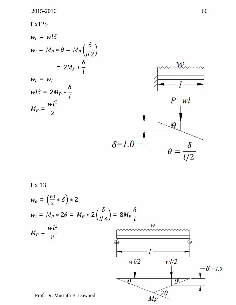
Ex12:-
푤 = 푤푙훿
푤 = 푀 ∗ 휃 = 푀훿푙/2
= 2푀 ∗훿푙
푤 = 푤
푤푙훿 = 2푀 ∗훿푙
푀 =푤푙
2
Ex 13
푤 = ∗ 훿 ∗ 2
푤 = 푀 ∗ 2휃 = 푀 ∗ 2훿푙/4 = 8푀
훿푙
푀 =푤푙
8
2015-2016 67
Prof. Dr. Mustafa B. Dawood Dr. Bilal Ismaeel Al-Shraify
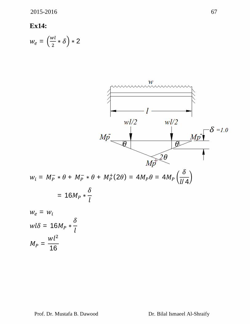
Ex14:
푤 = ∗ 훿 ∗ 2
푤 = 푀 ∗ 휃 + 푀 ∗ 휃 + 푀 (2휃) = 4푀 휃 = 4푀훿푙/4
= 16푀 ∗훿푙
푤 = 푤
푤푙훿 = 16푀 ∗훿푙
푀 =푤푙16
2015-2016 68
Prof. Dr. Mustafa B. Dawood Dr. Bilal Ismaeel Al-Shraify
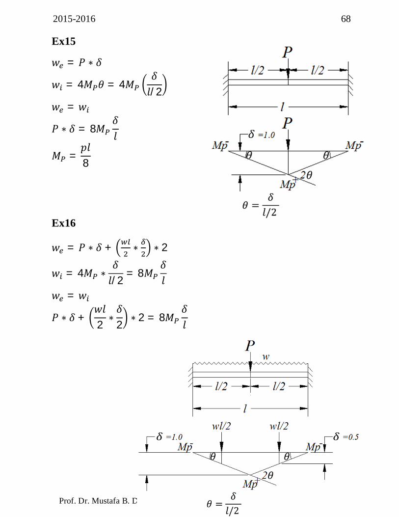
Ex15
푤 = 푃 ∗ 훿
푤 = 4푀 휃 = 4푀훿푙/2
푤 = 푤
푃 ∗ 훿 = 8푀훿푙
푀 =푝푙8
Ex16
푤 = 푃 ∗ 훿 + ∗ ∗ 2
푤 = 4푀 ∗훿푙/2 = 8푀
훿푙
푤 = 푤
푃 ∗ 훿 +푤푙2 ∗
훿2 ∗ 2 = 8푀
훿푙
2015-2016 69
Prof. Dr. Mustafa B. Dawood Dr. Bilal Ismaeel Al-Shraify
푀 =푤푙16 +
푝푙8
2015-2016 70
Prof. Dr. Mustafa B. Dawood Dr. Bilal Ismaeel Al-Shraify
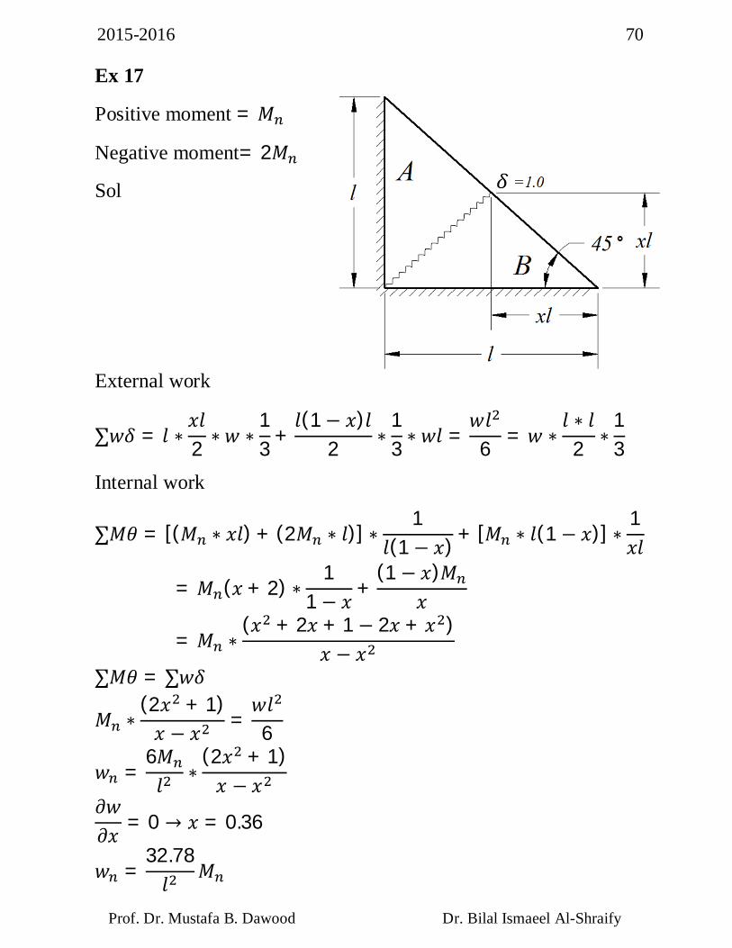
Ex 17
Positive moment = 푀
Negative moment= 2푀
Sol
External work
∑푤훿 = 푙 ∗푥푙2 ∗ 푤 ∗
13 +
푙(1 − 푥)푙2 ∗
13 ∗ 푤푙 =
푤푙6 = 푤 ∗
푙 ∗ 푙2 ∗
13
Internal work
∑푀휃 = [(푀 ∗ 푥푙) + (2푀 ∗ 푙)] ∗1
푙(1 − 푥) + [푀 ∗ 푙(1 − 푥)] ∗1푥푙
= 푀 (푥 + 2) ∗1
1 − 푥 +(1 − 푥)푀
푥
= 푀 ∗(푥 + 2푥 + 1 − 2푥 + 푥 )
푥 − 푥
∑푀휃 = ∑푤훿
푀 ∗(2푥 + 1)푥 − 푥 =
푤푙6
푤 =6푀푙 ∗
(2푥 + 1)푥 − 푥
휕푤휕푥 = 0 → 푥 = 0.36
푤 =32.78푙 푀
2015-2016 71
Prof. Dr. Mustafa B. Dawood Dr. Bilal Ismaeel Al-Shraify
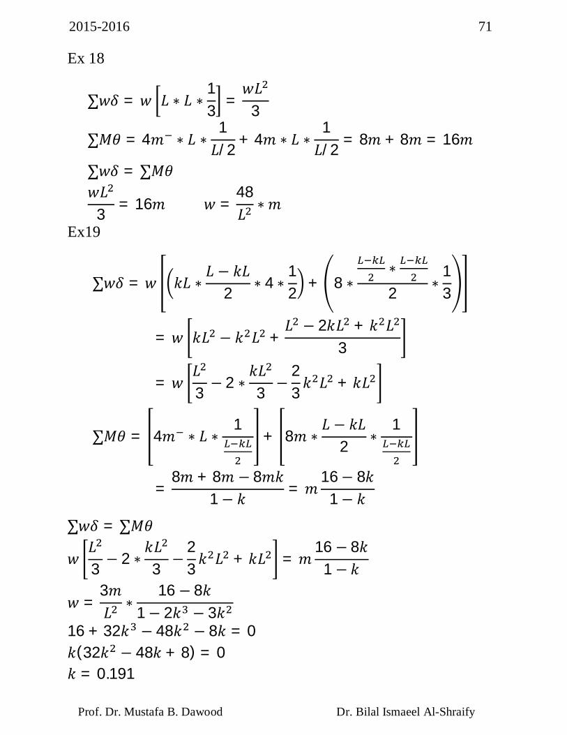
Ex 18
∑푤훿 = 푤 퐿 ∗ 퐿 ∗13 =
푤퐿3
∑푀휃 = 4푚 ∗ 퐿 ∗1퐿/2 + 4푚 ∗ 퐿 ∗
1퐿/2 = 8푚 + 8푚 = 16푚
∑푤훿 = ∑푀휃 푤퐿
3 = 16푚 푤 =48퐿 ∗ 푚
Ex19
∑푤훿 = 푤 푘퐿 ∗퐿 − 푘퐿
2 ∗ 4 ∗12 + 8 ∗
∗2 ∗
13
= 푤 푘퐿 − 푘 퐿 +퐿 − 2푘퐿 + 푘 퐿
3
= 푤퐿3 − 2 ∗
푘퐿3 −
23 푘 퐿 + 푘퐿
∑푀휃 = 4푚 ∗ 퐿 ∗1
+ 8푚 ∗퐿 − 푘퐿
2 ∗1
=8푚 + 8푚 − 8푚푘
1 − 푘 = 푚16 − 8푘
1 − 푘
∑푤훿 = ∑푀휃
푤퐿3 − 2 ∗
푘퐿3 −
23 푘 퐿 + 푘퐿 = 푚
16 − 8푘1 − 푘
푤 =3푚퐿 ∗
16 − 8푘1 − 2푘 − 3푘
16 + 32푘 − 48푘 − 8푘 = 0 푘(32푘 − 48푘 + 8) = 0 푘 = 0.191