Embed Size (px)
Citation preview

7/29/2019 2013 Predation Study on the Don Pedro Project
http://slidepdf.com/reader/full/2013-predation-study-on-the-don-pedro-project 1/71
PREDATION
STUDY REPORT
DON PEDRO PROJECT
FERC NO. 2299
Prepared for:
Turlock Irrigation District – Turlock, California
Modesto Irrigation District – Modesto, California
Prepared by:
FISHBIO
January 2013
7/29/2019 2013 Predation Study on the Don Pedro Project
http://slidepdf.com/reader/full/2013-predation-study-on-the-don-pedro-project 2/71
W&AR-07 i Initial Study Report
Predation Don Pedro Project, FERC No. 2299
Predation
Study Report
TABLE OF CONTENTS
Section No. Description Page No.
1.0 INTRODUCTION.......................................................................................................... 1-1 1.1 General Description of the Don Pedro Project .................................................... 1-1 1.2 Relicensing Process ............................................................................................. 1-3 1.3 Study Plan ............................................................................................................ 1-3
2.0 STUDY GOALS AND OBJECTIVES .......................................................................... 2-1 3.0 STUDY AREA ................................................................................................................ 3-1 4.0 METHODOLOGY ........................................................................................................ 4-3
4.1 River Conditions .................................................................................................. 4-3 4.2 Predator Abundance ............................................................................................. 4-3
4.2.1 Sampling Methods ................................................................................... 4-3 4.2.1.1 Sampling Locations ............................................................... 4-3 4.2.1.2 Habitat Measurements ........................................................... 4-3 4.2.1.3 Electrofishing Methods .......................................................... 4-6
4.2.2
Data Analysis ........................................................................................... 4-6
4.2.2.1 Depletion Estimates ............................................................... 4-6 4.2.2.2 Density Estimates ................................................................... 4-7 4.2.2.3 River Wide Abundance Estimates ......................................... 4-8
4.3 Predation Rate ...................................................................................................... 4-8 4.3.1 Collection of Stomach Samples ............................................................... 4-8 4.3.2 Identification of Prey Items ..................................................................... 4-9 4.3.3 Data Analysis ......................................................................................... 4-11
4.3.3.1 Water Temperatures Prior to Time of Capture .................... 4-11 4.3.3.2 Gastric Evacuation Rates ..................................................... 4-11 4.3.3.3 Predation Ratio and Predation Rates.................................... 4-11
4.4 Predator Movement Tracking ............................................................................ 4-12 4.4.1 Acoustic Tag System Overview ............................................................. 4-12 4.4.2 Predator Tagging .................................................................................... 4-13

7/29/2019 2013 Predation Study on the Don Pedro Project
http://slidepdf.com/reader/full/2013-predation-study-on-the-don-pedro-project 3/71
Table of Contents
W&AR-07 ii Initial Study Report
Predation Don Pedro Project, FERC No. 2299
4.4.3 Chinook Salmon Releases...................................................................... 4-14 4.4.3.1 Acoustic Tagging of Chinook Salmon ................................. 4-14 4.4.3.2 Photonic Marking of Chinook Salmon ................................ 4-16 4.4.3.3 Transport and Holding of Chinook Salmon ......................... 4-16 4.4.3.4 Releases of Tagged and Marked Chinook Salmon .............. 4-16
4.4.4 Acoustic Array Deployment and Maintenance ...................................... 4-17 5.0 RESULTS ....................................................................................................................... 5-1
5.1 River Conditions .................................................................................................. 5-1 5.2 Predator Abundance ............................................................................................. 5-2
5.2.1 Habitat Measurements ............................................................................. 5-2 5.2.2 Site-Specific Abundance and Density ..................................................... 5-3 5.2.3 River Wide Abundance Estimates ........................................................... 5-5
5.3 Predation Rate ...................................................................................................... 5-5 5.3.1 Diet Composition ..................................................................................... 5-6 5.3.2 Predation of juvenile Chinook salmon ..................................................... 5-8 5.3.3 Differences between sampling events and habitat types.......................... 5-9 5.3.4 Water temperatures ................................................................................ 5-10 5.3.5 Predation rates on juvenile Chinook salmon ......................................... 5-10
5.4 Predator Movement Tracking ............................................................................ 5-13 5.4.1 Predator Tagging .................................................................................... 5-13 5.4.2 Detections of Acoustic Tagged Fish ...................................................... 5-15
5.4.2.1 Transit Times of Acoustic Tagged Chinook Salmon ........... 5-21 5.4.2.2 Residence Times Within Special Run-Pools ....................... 5-23 5.4.2.3 Riffle Monitoring ................................................................. 5-25
6.0 DISCUSSION AND FINDINGS ................................................................................... 6-1 6.1 Predator Abundance ............................................................................................. 6-1
6.1.1 Riverwide Abundance Estimates ............................................................. 6-1 6.1.2 Site-specific Abundance Estimates .......................................................... 6-1 6.1.3 Smallmouth and Largemouth Bass Densities .......................................... 6-2 6.1.4 General Spatial Distribution .................................................................... 6-2
6.2 Predation Rate ...................................................................................................... 6-2 6.2.1 Diet Composition ..................................................................................... 6-4
6.3 Synthesizing Abundance and Predation Rates ..................................................... 6-4

7/29/2019 2013 Predation Study on the Don Pedro Project
http://slidepdf.com/reader/full/2013-predation-study-on-the-don-pedro-project 4/71
Table of Contents
W&AR-07 iii Initial Study Report
Predation Don Pedro Project, FERC No. 2299
6.4 Differential Habitat Use ....................................................................................... 6-6 6.5 Potential Additional Studies to Be Conducted in 2013 ....................................... 6-6
7.0 STUDY VARIANCES AND MODIFICATIONS ........................................................ 7-1 8.0 REFERENCES ............................................................................................................... 8-1
List of Figures
Figure No. Description Page No.
Figure 1.1-1. Don Pedro Project location. ................................................................................. 1-2 Figure 3.0-1. Map of study area................................................................................................. 3-2 Figure 4.2-1. Map of the predator abundance sampling sites. ................................................... 4-5 Figure 4.3-1. Predation rate sampling sites. ............................................................................ 4-10 Figure 4.4-1. Acoustic array deployment locations. ................................................................ 4-15 Figure 5.1-1. Daily mean discharge at La Grange (LGN) March 1 through August 31
and timing of sampling events. ............................................................................ 5-1 Figure 5.1-2. Daily minimum and maximum water temperatures at Roberts Ferry (RM
39.4) and Grayson (RM 5.0) March 1 through August 31 and timing of
sampling events. ................................................................................................... 5-2 Figure 5.3-1. Number of identifiable prey items observed in stomach samples (n = 246)
collected in the lower Tuolumne River. Invertebrates (insects and crayfish)
and fish (various species) made up the majority of identifiable prey items. ....... 5-7 Figure 5.3-2. Number of stomach samples (n = 246) that contained at least one of each
type of prey item collected on the lower Tuolumne River. ................................. 5-7 Figure 5.3-3. Number of prey items (by order) observed in stomach samples (n = 246)
collected in the lower Tuolumne River. ............................................................... 5-8 Figure 5.3-4. Lengths of captured smallmouth bass, largemouth bass, striped bass, and
Sacramento pikeminnow that consumed juvenile Chinook salmon (dark
bars) and those that did not (light bars). .............................................................. 5-9 Figure 5.3-5. Comparison of estimated predation frequency and 95 percent confidence
intervals by habitat type and event. Statistically significant difference
denoted by “*”and “NS” indicates no significant difference............................. 5-10 Figure 5.4-1. Densities of acoustic tagged Chinook salmon and predators in SRP 6 at
2,100 cfs (Chinook salmon: blue, largemouth bass: orange, and striped
bass: red). Darker shaded areas represent 90th
percentile, and lighter
shading represents 95th percentile densities. Note: where polygons overlap,not all species present may be visible. ............................................................... 5-16
Figure 5.4-2. Densities of acoustic tagged Chinook salmon and predators in SRP 10 at
2,100 cfs (Chinook salmon: blue, largemouth bass: orange, smallmouth
bass: green, and striped bass: red). Darker shaded areas represent 90th
percentile, and lighter shading represents 95
thpercentile densities. Note:
where polygons overlap, not all species present may be visible. ....................... 5-17
7/29/2019 2013 Predation Study on the Don Pedro Project
http://slidepdf.com/reader/full/2013-predation-study-on-the-don-pedro-project 5/71
Table of Contents
W&AR-07 iv Initial Study Report
Predation Don Pedro Project, FERC No. 2299
Figure 5.4-3. SRP 6 Low flow densities of tagged Chinook and predators (Chinook
salmon: blue, largemouth bass: orange, smallmouth bass: green, striped bass: red, and Sacramento pikeminnow: purple). Darker shaded areas
represent 90th
percentile, and lighter shading represents 95th
percentile
densities. Note: where polygons overlap, not all species present may be
visible. ................................................................................................................ 5-18
Figure 5.4-4. SRP 10 Low flow densities of tagged Chinook and predators (Chinook
salmon: blue, largemouth bass: orange, smallmouth bass: green, and
striped bass: red). Darker shaded areas represent 90th
percentile, andlighter shading represents 95
thpercentile densities. Note: where polygons
overlap, not all species present may be visible. ................................................. 5-19 Figure 5.4-5. SRP 6 Mid flow densities of tagged Chinook and predators (Chinook
salmon: blue, largemouth bass: orange, smallmouth bass: green, andstriped bass: red). Darker shaded areas represent 90
thpercentile, and
lighter shading represents 95th
percentile densities. Note: where polygons
overlap, not all species present may be visible. ................................................. 5-20 Figure 5.4-6. SRP 10 Mid flow densities of tagged Chinook and predators (Chinook
salmon: blue, largemouth bass: orange, smallmouth bass: green, and
striped bass: red). Darker shaded areas represent 90th
percentile, and
lighter shading represents 95th
percentile densities. Note: where polygonsoverlap, not all species present may be visible. ................................................. 5-21
Figure 5.4-7. Transit times from Hickman Bridge to SRP 6 of acoustic tagged juvenile
Chinook salmon (n = 109 total; n = 59 at 2,100 cfs; n = 30 at 280 cfs; and,n = 20 at 415 cfs). .............................................................................................. 5-22
Figure 5.4-8. Transit times from SRP 6 to SRP 10 of acoustic tagged juvenile Chinook
salmon (n = 53 total; n = 40 at 2,100 cfs; n = 11 at 280 cfs; and, n = 2 at
415 cfs)............................................................................................................... 5-23
Figure 5.4-9. Residence times (in minutes) at SRP 6 of acoustic tagged juvenile
Chinook salmon (n = 109 total; n = 59 for 2,100 cfs; n = 30 for 280 cfs;and, n = 20 for 415 cfs). ..................................................................................... 5-24
Figure 5.4-10. Residence times (in minutes) at SRP 10 of acoustic tagged juvenile
Chinook salmon (n = 55 total; n = 42 for 2,100 cfs; n = 11 for 280 cfs;
and, n = 2 for 415 cfs). ....................................................................................... 5-25
List of Tables
Table No. Description Page No.
Table 4.3-1. Location information of temperature recorders and predation rate sampling
locations on the lower Tuolumne River during Spring and Summer 2012. ...... 4-11 Table 4.4-1 Releases of acoustic tagged Chinook salmon. ................................................... 4-17 Table 5.2-1. Habitat sizes of sampled units in the lower Tuolumne River measured in
GIS. ...................................................................................................................... 5-2
7/29/2019 2013 Predation Study on the Don Pedro Project
http://slidepdf.com/reader/full/2013-predation-study-on-the-don-pedro-project 6/71
Table of Contents
W&AR-07 v Initial Study Report
Predation Don Pedro Project, FERC No. 2299
Table 5.2-2. Site-specific depletion estimates of largemouth bass >150 mm and
associated density estimates on the lower Tuolumne River during summer 2012...................................................................................................................... 5-3
Table 5.2-3. Site-specific depletion estimates of smallmouth bass >150 mm and
associated density estimates on the lower Tuolumne River during summer
2012...................................................................................................................... 5-3 Table 5.2-4. Site-specific depletion estimates of striped bass >150 mm and associated
density estimates on the lower Tuolumne River during summer 2012. .............. 5-4 Table 5.2-5. Site-specific depletion estimates of Sacramento pikeminnow >150 mm
and associated density estimates on the lower Tuolumne River duringsummer 2012. ....................................................................................................... 5-4
Table 5.2-6. Abundance estimates and associated standard errors based on estimated
densities (by area and shoreline length of run-pools and special run-pools)of each target species on the lower Tuolumne River (RM 0 to RM 39.4). .......... 5-5
Table 5.3-1. Numbers of predatory fish (> 150 mm FL) stomachs sampled and number
and percentage of predatory fish with empty stomachs duringelectrofishing on the lower Tuolumne River during spring 2012. ....................... 5-6 Table 5.3-2. Summary of largemouth bass (LMB), smallmouth bass (SMB), striped
bass (STB), and Sacramento pikeminnow (SASQ) predation of juvenile
Chinook salmon in the lower Tuolumne River during March and May
2012.................................................................................................................... 5-12 Table 5.4-1. Summary of predator species acoustically tagged. ............................................ 5-13 Table 5.4-2. Summary of fate determinations for acoustic tagged Chinook salmon in
SRP 6 and SRP 10, and river flow at La Grange, and water temperature at
Roberts Ferry. .................................................................................................... 5-15 Table 5.4-3. Summary of overlap in habitat use at the 90
thpercentile between acoustic
tagged Chinook salmon and predators in SRP 6 and SRP 10. ........................... 5-21 Table 6.3-1. Estimated cumulative impact of predation in the lower Tuolumne River
between RM 30.3 and RM 5.1 under a low predation rate (gastric
evacuation time set at 20-hours) by length of migratory period of juvenile
Chinook salmon. .................................................................................................. 6-5
List of Attachments
Attachment A Habitat size versus site-specific abundance estimates of target species in allsampled units in the Tuolumne River
7/29/2019 2013 Predation Study on the Don Pedro Project
http://slidepdf.com/reader/full/2013-predation-study-on-the-don-pedro-project 7/71
W&AR-07 vi Initial Study Report
Predation Don Pedro Project, FERC No. 2299
List of Acronyms
ac ................................acres
ACEC .........................Area of Critical Environmental Concern
AF ..............................acre-feetACOE .........................U.S. Army Corps of Engineers
ADA ...........................Americans with Disabilities Act
ALJ .............................Administrative Law Judge
APE ............................Area of Potential Effect
ARMR ........................Archaeological Resource Management Report
ATR…………………Acoustic Tag Receiver
ATS…………………Acoustic Tag Tracking System
BA ..............................Biological Assessment
BDCP .........................Bay-Delta Conservation Plan
BLM ...........................U.S. Department of the Interior, Bureau of Land Management
BLM-S .......................Bureau of Land Management – Sensitive Species
BMI ............................Benthic macroinvertebrates
BMP ...........................Best Management Practices
BO ..............................Biological Opinion
CalEPPC ....................California Exotic Pest Plant Council
CalSPA .......................California Sports Fisherman Association
CAS ............................California Academy of Sciences
CCC............................Criterion Continuous Concentrations
CCIC ..........................Central California Information Center
CCSF ..........................City and County of San Francisco
CCVHJV ....................California Central Valley Habitat Joint Venture
CD ..............................Compact Disc
CDBW........................California Department of Boating and Waterways
CDEC .........................California Data Exchange Center
CDFA .........................California Department of Food and Agriculture
CDFG .........................California Department of Fish and Game (as of January 2013, Departmentof Fish and Wildlife)
CDMG........................California Division of Mines and Geology
7/29/2019 2013 Predation Study on the Don Pedro Project
http://slidepdf.com/reader/full/2013-predation-study-on-the-don-pedro-project 8/71
List of Acronyms
W&AR-07 vii Initial Study Report
Predation Don Pedro Project, FERC No. 2299
CDOF .........................California Department of Finance
CDPH .........................California Department of Public Health
CDPR .........................California Department of Parks and Recreation
CDSOD ......................California Division of Safety of Dams
CDWR........................California Department of Water Resources
CE ..............................California Endangered Species
CEII ............................Critical Energy Infrastructure Information
CEQA .........................California Environmental Quality Act
CESA .........................California Endangered Species Act
CFR ............................Code of Federal Regulations
cfs ...............................cubic feet per second
CGS ............................California Geological Survey
CMAP ........................California Monitoring and Assessment Program
CMC ...........................Criterion Maximum Concentrations
CNDDB......................California Natural Diversity Database
CNPS..........................California Native Plant Society
CORP .........................California Outdoor Recreation Plan
CPUE .........................Catch Per Unit Effort
CRAM ........................California Rapid Assessment Method
CRLF..........................California Red-Legged FrogCRRF .........................California Rivers Restoration Fund
CSAS..........................Central Sierra Audubon Society
CSBP ..........................California Stream Bioassessment Procedure
CT ..............................California Threatened Species
CTR ............................California Toxics Rule
CTS ............................California Tiger Salamander
CVRWQCB ...............Central Valley Regional Water Quality Control Board
CWA ..........................Clean Water Act
CWHR........................California Wildlife Habitat Relationship
Districts ......................Turlock Irrigation District and Modesto Irrigation District
DLA ...........................Draft License Application
DPRA .........................Don Pedro Recreation Agency
DPS ............................Distinct Population Segment
7/29/2019 2013 Predation Study on the Don Pedro Project
http://slidepdf.com/reader/full/2013-predation-study-on-the-don-pedro-project 9/71
List of Acronyms
W&AR-07 viii Initial Study Report
Predation Don Pedro Project, FERC No. 2299
EA ..............................Environmental Assessment
EC ..............................Electrical Conductivity
EFH ............................Essential Fish Habitat
EIR .............................Environmental Impact Report
EIS..............................Environmental Impact Statement
EPA ............................U.S. Environmental Protection Agency
ESA ............................Federal Endangered Species Act
ESRCD .......................East Stanislaus Resource Conservation District
ESU ............................Evolutionary Significant Unit
EWUA........................Effective Weighted Useable Area
FERC..........................Federal Energy Regulatory Commission
FFS .............................Foothills Fault System
FL ...............................Fork length
FMU ...........................Fire Management Unit
FOT ............................Friends of the Tuolumne
FPC ............................Federal Power Commission
ft/mi ............................feet per mile
FWCA ........................Fish and Wildlife Coordination Act
FYLF ..........................Foothill Yellow-Legged Frog
g..................................gramsGIS .............................Geographic Information System
GLO ...........................General Land Office
GPS ............................Global Positioning System
HCP ............................Habitat Conservation Plan
HHWP ........................Hetch Hetchy Water and Power
HORB ........................Head of Old River Barrier
HPMP .........................Historic Properties Management Plan
ILP..............................Integrated Licensing Process
ISR .............................Initial Study Report
ITA .............................Indian Trust Assets
kV ...............................kilovolt
m ................................meters
M&I............................Municipal and Industrial

7/29/2019 2013 Predation Study on the Don Pedro Project
http://slidepdf.com/reader/full/2013-predation-study-on-the-don-pedro-project 10/71
List of Acronyms
W&AR-07 ix Initial Study Report
Predation Don Pedro Project, FERC No. 2299
MCL ...........................Maximum Contaminant Level
mg/kg .........................milligrams/kilogram
mg/L ...........................milligrams per liter
mgd ............................million gallons per day
mi ...............................miles
mi2..............................square miles
MID ............................Modesto Irrigation District
MOU ..........................Memorandum of Understanding
MRH………………...Merced River Hatchery
MSCS .........................Multi-Species Conservation Strategy
msl ..............................mean sea level
MVA ..........................Megavolt Ampere
MW ............................megawatt
MWh ..........................megawatt hour
mya .............................million years ago
NAE ...........................National Academy of Engineering
NAHC ........................Native American Heritage Commission
NAS............................National Academy of Sciences
NAVD 88 ...................North American Vertical Datum of 1988
NAWQA ....................National Water Quality Assessment NCCP .........................Natural Community Conservation Plan
NEPA .........................National Environmental Policy Act
ng/g ............................nanograms per gram
NGOs .........................Non-Governmental Organizations
NHI ............................Natural Heritage Institute
NHPA .........................National Historic Preservation Act
NISC ..........................National Invasive Species Council
NMFS .........................National Marine Fisheries Service
NOAA ........................National Oceanic and Atmospheric Administration
NOI ............................Notice of Intent
NPS ............................U.S. Department of the Interior, National Park Service
NRCS .........................National Resource Conservation Service
NRHP .........................National Register of Historic Places

7/29/2019 2013 Predation Study on the Don Pedro Project
http://slidepdf.com/reader/full/2013-predation-study-on-the-don-pedro-project 11/71
List of Acronyms
W&AR-07 x Initial Study Report
Predation Don Pedro Project, FERC No. 2299
NRI .............................Nationwide Rivers Inventory
NTU ...........................Nephelometric Turbidity Unit
NWI............................National Wetland Inventory
NWIS .........................National Water Information System
NWR ..........................National Wildlife Refuge
NGVD 29 ...................National Geodetic Vertical Datum of 1929
O&M ..........................operation and maintenance
OEHHA......................Office of Environmental Health Hazard Assessment
ORV ...........................Outstanding Remarkable Value
PAD............................Pre-Application Document
PDO............................Pacific Decadal Oscillation
PEIR ...........................Program Environmental Impact Report
PGA............................Peak Ground Acceleration
PHG............................Public Health Goal
PM&E ........................Protection, Mitigation and Enhancement
PMF............................Probable Maximum Flood
POAOR ......................Public Opinions and Attitudes in Outdoor Recreation
ppb..............................parts per billion
ppm ............................parts per million
PSP .............................Proposed Study PlanQA ..............................Quality Assurance
QC ..............................Quality Control
RA ..............................Recreation Area
RBP ............................Rapid Bioassessment Protocol
Reclamation ...............U.S. Department of the Interior, Bureau of Reclamation
RM .............................River Mile
RMP ...........................Resource Management Plan
RP ...............................Relicensing Participant
RSP ............................Revised Study Plan
RST ............................Rotary Screw Trap
RWF ...........................Resource-Specific Work Groups
RWG ..........................Resource Work Group
RWQCB .....................Regional Water Quality Control Board

7/29/2019 2013 Predation Study on the Don Pedro Project
http://slidepdf.com/reader/full/2013-predation-study-on-the-don-pedro-project 12/71
List of Acronyms
W&AR-07 xi Initial Study Report
Predation Don Pedro Project, FERC No. 2299
SC ...............................State candidate for listing under CESA
SCD ............................State candidate for delisting under CESA
SCE ............................State candidate for listing as endangered under CESA
SCT ............................State candidate for listing as threatened under CESA
SD1 ............................Scoping Document 1
SD2 ............................Scoping Document 2
SE ...............................State Endangered Species under the CESA
SFP .............................State Fully Protected Species under CESA
SFPUC .......................San Francisco Public Utilities Commission
SHPO .........................State Historic Preservation Office
SJRA ..........................San Joaquin River Agreement
SJRGA .......................San Joaquin River Group Authority
SJTA ..........................San Joaquin River Tributaries Authority
SPD ............................Study Plan Determination
SRA ............................State Recreation Area
SRMA ........................Special Recreation Management Area or Sierra Resource ManagementArea (as per use)
SRMP .........................Sierra Resource Management Plan
SRP ............................Special Run Pools
SSC ............................State species of special concern
ST ...............................California Threatened Species under the CESA
STORET ....................Storage and Retrieval
SWAMP .....................Surface Water Ambient Monitoring Program
SWE ...........................Snow-Water Equivalent
SWRCB......................State Water Resources Control Board
TAC............................Technical Advisory Committee
TAF ............................thousand acre-feet
TCP ............................Traditional Cultural PropertiesTDS ............................Total Dissolved Solids
TID .............................Turlock Irrigation District
TMDL ........................Total Maximum Daily Load
TOC............................Total Organic Carbon
TRT ............................Tuolumne River Trust

7/29/2019 2013 Predation Study on the Don Pedro Project
http://slidepdf.com/reader/full/2013-predation-study-on-the-don-pedro-project 13/71
List of Acronyms
W&AR-07 xii Initial Study Report
Predation Don Pedro Project, FERC No. 2299
TRTAC ......................Tuolumne River Technical Advisory Committee
UC ..............................University of California
USDA .........................U.S. Department of Agriculture
USDOC ......................U.S. Department of Commerce
USDOI .......................U.S. Department of the Interior
USFS ..........................U.S. Department of Agriculture, Forest Service
USFWS ......................U.S. Department of the Interior, Fish and Wildlife Service
USGS .........................U.S. Department of the Interior, Geological Survey
USR ............................Updated Study Report
UTM ...........................Universal Transverse Mercator
VAMP ........................Vernalis Adaptive Management Plan
VELB .........................Valley Elderberry Longhorn Beetle
VRM ..........................Visual Resource Management
WPT ...........................Western Pond Turtle
WSA ...........................Wilderness Study Area
WSIP ..........................Water System Improvement Program
WWTP .......................Wastewater Treatment Plant
WY .............................water year
μS/cm .........................microSeimens per centimeter

7/29/2019 2013 Predation Study on the Don Pedro Project
http://slidepdf.com/reader/full/2013-predation-study-on-the-don-pedro-project 14/71
W&AR-07 1-1 Initial Study Report
Predation Don Pedro Project, FERC No. 2299
1.0 INTRODUCTION
1.1 General Description of the Don Pedro Project
Turlock Irrigation District (TID) and Modesto Irrigation District (MID) (collectively, the
Districts) are the co-licensees of the 168-megawatt (MW) Don Pedro Project (Project) located onthe Tuolumne River in western Tuolumne County in the Central Valley region of California.
The Don Pedro Dam is located at river mile (RM) 54.8 and the Don Pedro Reservoir formed by
the dam extends 24-miles upstream at the normal maximum water surface elevation of 830 ft
above mean sea level (msl; NGVD 29). At elevation 830 ft, the reservoir stores over 2,000,000acre-feet (AF) of water and has a surface area slightly less than 13,000 acres (ac). The watershed
above Don Pedro Dam is approximately 1,533 square miles (mi2).
Both TID and MID are local public agencies authorized under the laws of the State of California
to provide water supply for irrigation and municipal and industrial (M&I) uses and to provide
retail electric service. The Project serves many purposes including providing water storage for
the beneficial use of irrigation of over 200,000 ac of prime Central Valley farmland and for theuse of M&I customers in the City of Modesto (population 210,000). Consistent with the
requirements of the Raker Act passed by Congress in 1913 and agreements between the Districtsand City and County of San Francisco (CCSF), the Project reservoir also includes a “water bank”
of up to 570,000 AF of storage. CCSF may use the water bank to more efficiently manage the
water supply from its Hetch Hetchy water system while meeting the senior water rights of the
Districts. CCSF’s “water bank” within Don Pedro Reservoir provides significant benefits for its2.6 million customers in the San Francisco Bay Area.
The Project also provides storage for flood management purposes in the Tuolumne and SanJoaquin rivers in coordination with the U.S. Army Corps of Engineers (ACOE). Other important
uses supported by the Project are recreation, protection of the anadromous fisheries in the lower Tuolumne River, and hydropower generation.
The Project Boundary extends from approximately one mile downstream of the dam to
approximately RM 79 upstream of the dam. Upstream of the dam, the Project Boundary runs
generally along the 855 ft contour interval which corresponds to the top of the Don Pedro Dam.The Project Boundary encompasses approximately 18,370 ac with 78 percent of the lands owned
jointly by the Districts and the remaining 22 percent (approximately 4,000 ac) is owned by the
United States and managed as a part of the U.S. Bureau of Land Management (BLM) SierraResource Management Area.
The primary Project facilities include the 580-foot-high Don Pedro Dam and Reservoir completed in 1971; a four-unit powerhouse situated at the base of the dam; related facilities
including the Project spillway, outlet works, and switchyard; four dikes (Gasburg Creek Dike
and Dikes A, B, and C); and three developed recreational facilities (Fleming Meadows, BlueOaks, and Moccasin Point Recreation Areas). The location of the Project and its primary
facilities is shown in Figure 1.1-1.

7/29/2019 2013 Predation Study on the Don Pedro Project
http://slidepdf.com/reader/full/2013-predation-study-on-the-don-pedro-project 15/71
1.0 Introduction
W&AR-07 1-2 Initial Study Report
Predation Don Pedro Project, FERC No. 2299
Figure 1.1-1. Don Pedro Project location.

7/29/2019 2013 Predation Study on the Don Pedro Project
http://slidepdf.com/reader/full/2013-predation-study-on-the-don-pedro-project 16/71
1.0 Introduction
W&AR-07 1-3 Initial Study Report
Predation Don Pedro Project, FERC No. 2299
1.2 Relicensing Process
The current FERC license for the Project expires on April 30, 2016, and the Districts will applyfor a new license no later than April 30, 2014. The Districts began the relicensing process by
filing a Notice of Intent and Pre-Application Document (PAD) with FERC on February 10, 2011,
following the regulations governing the Integrated Licensing Process (ILP). The Districts’ PADincluded descriptions of the Project facilities, operations, license requirements, and Project landsas well as a summary of the extensive existing information available on Project area resources.
The PAD also included ten draft study plans describing a subset of the Districts’ proposed
relicensing studies. The Districts then convened a series of Resource Work Group meetings,engaging agencies and other relicensing participants in a collaborative study plan development
process culminating in the Districts’ Proposed Study Plan (PSP) and Revised Study Plan (RSP)
filings to FERC on July 25, 2011 and November 22, 2011, respectively.
On December 22, 2011, FERC issued its Study Plan Determination (SPD) for the Project,
approving, or approving with modifications, 34 studies proposed in the RSP that addressed
Cultural and Historical Resources, Recreational Resources, Terrestrial Resources, and Water andAquatic Resources. In addition, as required by the SPD, the Districts filed three new study plans
(W&AR-18, W&AR-19, and W&AR-20) on February 28, 2012 and one modified study plan
(W&AR-12) on April 6, 2012. Prior to filing these plans with FERC, the Districts consultedwith relicensing participants on drafts of the plans. FERC approved or approved with
modifications these four studies on July 25, 2012.
Following the SPD, a total of seven studies (and associated study elements) that were either not
adopted in the SPD, or were adopted with modifications, formed the basis of Study Dispute
proceedings. In accordance with the ILP, FERC convened a Dispute Resolution Panel on April17, 2012 and the Panel issued its findings on May 4, 2012. On May 24, 2012, the Director of
FERC issued his Formal Study Dispute Determination, with additional clarifications related tothe Formal Study Dispute Determination issued on August 17, 2012.
This study report describes the objectives, methods, and results of the Predation Study
(W&AR-07) as implemented by the Districts in accordance with FERC’s SPD and subsequent
study modifications and clarifications. Documents relating to the Project relicensing are publiclyavailable on the Districts’ relicensing website at www.donpedro-relicensing.com.
1.3 Study Plan
FERC’s Scoping Document 2 identified potential effects of the Project on fish populations in
Project-affected reaches. The continued operation and maintenance (O&M) of the Project maycontribute to cumulative effects on salmonid fish habitat in the Tuolumne River downstream of
La Grange Dam, including the effects of predation on survival of juvenile Chinook salmon andO. mykiss in the lower Tuolumne River.
FERC’s SPD approved with modifications the Districts’ Predation study plan as provided in the
Districts’ RSP filing. In its SPD, FERC ordered that the Districts include the following
provisions: (1) a goal to ensure the ratio of tag to fish weight is less than five percent, (2) any

7/29/2019 2013 Predation Study on the Don Pedro Project
http://slidepdf.com/reader/full/2013-predation-study-on-the-don-pedro-project 17/71
1.0 Introduction
W&AR-07 1-4 Initial Study Report
Predation Don Pedro Project, FERC No. 2299
additional hatchery reared fish should be coded-wire-tagged, and (3) if the results of the
predation study and the FWS’s GIS floodplain inundation study suggest that a second year of study may be needed, the Districts should propose such a study in its initial study report or
explain why such a study is not needed.
7/29/2019 2013 Predation Study on the Don Pedro Project
http://slidepdf.com/reader/full/2013-predation-study-on-the-don-pedro-project 18/71
W&AR-07 2-1 Initial Study Report
Predation Don Pedro Project, FERC No. 2299
2.0 STUDY GOALS AND OBJECTIVES
The goal of this study was to increase understanding of the current effects of predation on rearing
and outmigrating juvenile Chinook salmon and O. mykiss in the lower Tuolumne River. The
study consisted of the following three components related to salmonid predation by native and
non-native species in the lower Tuolumne River:
(1) Predator abundance - estimate relative abundance of predator fish species such aslargemouth bass ( Micropterus salmoides), smallmouth bass ( Micropterus dolomieu),
Sacramento pikeminnow (Ptychocheilus grandis), and striped bass ( Morone saxitalis)
(2) Predation rate - update estimates of predation rate from previous surveys (e.g., TID/MID
1992)
(3) Predator movement tracking - determine relative habitat use by juvenile Chinook salmonand predator species at typical flows encountered during the juvenile salmonid
outmigration period.
7/29/2019 2013 Predation Study on the Don Pedro Project
http://slidepdf.com/reader/full/2013-predation-study-on-the-don-pedro-project 19/71
W&AR-07 3-1 Initial Study Report
Predation Don Pedro Project, FERC No. 2299
3.0 STUDY AREA
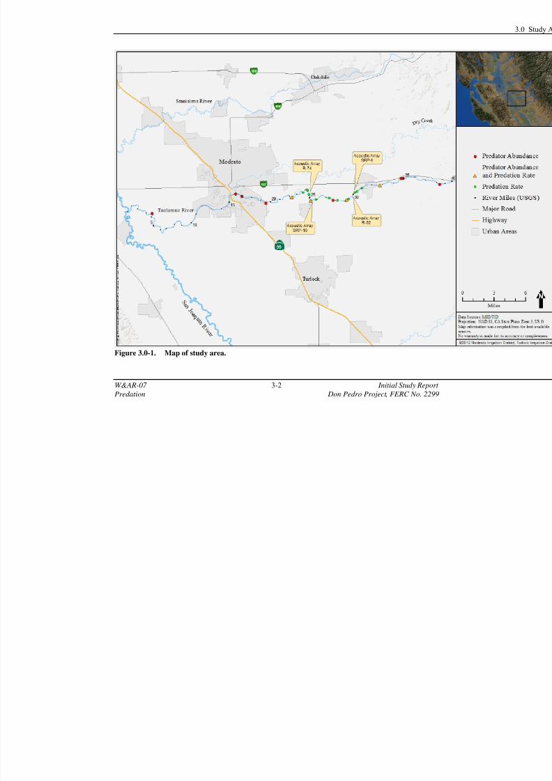
The study area includes the Tuolumne River from the La Grange Dam (RM 52) downstream to
the confluence with the San Joaquin River (RM 0) (Figure 3.0-1). Study sites were selected in
habitat units or river reaches that provide suitable habitat for predators and where predators have
been documented in prior studies (TID/MID 1992; Brown and Ford 2002; Stillwater Sciencesand McBain & Trush 2006). As the majority of predators in the lower Tuolumne River are non-
native and are most abundant downstream of approximately RM 31 (Brown and Ford 2002), andthe Section 10 permit issued by the National Marine Fisheries Service (NMFS) for take of
Central Valley Steelhead limited sampling to locations downstream of RM 31.5 during
September - March, predation study sites were generally concentrated in this downstream reach.
Specific locations of sampling sites are described in Sections 4.2, 4.3, and 4.4 of this report.
7/29/2019 2013 Predation Study on the Don Pedro Project
http://slidepdf.com/reader/full/2013-predation-study-on-the-don-pedro-project 20/71
W&AR-07 3-2 Initial Study Report
Predation Don Pedro Project, FERC No. 2299
Figure 3.0-1. Map of study area.
7/29/2019 2013 Predation Study on the Don Pedro Project
http://slidepdf.com/reader/full/2013-predation-study-on-the-don-pedro-project 21/71
W&AR-07 4-3 Initial Study Report
Predation Don Pedro Project, FERC No. 2299
4.0 METHODOLOGY
4.1 River Conditions
Provisional daily average flow data for the Tuolumne River at La Grange was obtained from the
U.S. Department of the Interior, Geological Survey (USGS) athttp://waterdata.usgs.gov/ca/nwis/uv/?site_no=11289650&agency_cd=USGS. Water
temperature data were obtained from hourly recording Hobo Pro v2 water temperature data
loggers (Onset Computer Corporation) maintained by the Districts at Roberts Ferry Bridge (RM
39.4), Hickman Bridge (RM 31.6), Waterford (RM 29.8), SRP 10 (RM 25.5), Tuolumne River Weir (RM 24.4), and Grayson (RM 5.0).
Daily instantaneous turbidity samples were collected at Waterford (RM 29.8), Tuolumne River Weir (RM 24.4), and Grayson (RM 5.0). Samples were also collected prior to electrofishing each
site sampled for predator abundance and predation rate.
4.2 Predator Abundance
4.2.1 Sampling Methods
4.2.1.1 Sampling Locations
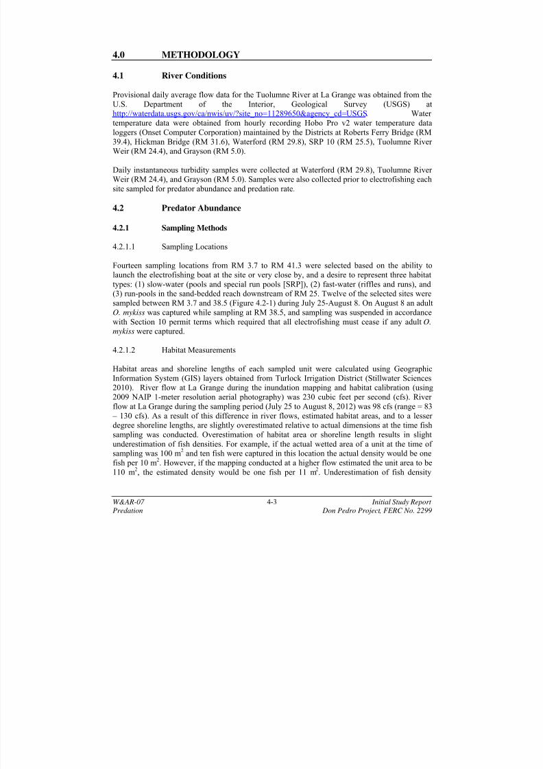
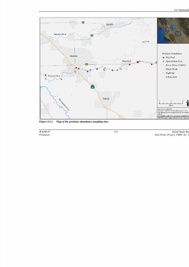
Fourteen sampling locations from RM 3.7 to RM 41.3 were selected based on the ability to
launch the electrofishing boat at the site or very close by, and a desire to represent three habitat
types: (1) slow-water (pools and special run pools [SRP]), (2) fast-water (riffles and runs), and(3) run-pools in the sand-bedded reach downstream of RM 25. Twelve of the selected sites were
sampled between RM 3.7 and 38.5 (Figure 4.2-1) during July 25-August 8. On August 8 an adult
O. mykiss was captured while sampling at RM 38.5, and sampling was suspended in accordancewith Section 10 permit terms which required that all electrofishing must cease if any adult O.
mykiss were captured.
4.2.1.2 Habitat Measurements
Habitat areas and shoreline lengths of each sampled unit were calculated using Geographic
Information System (GIS) layers obtained from Turlock Irrigation District (Stillwater Sciences2010). River flow at La Grange during the inundation mapping and habitat calibration (using
2009 NAIP 1-meter resolution aerial photography) was 230 cubic feet per second (cfs). River
flow at La Grange during the sampling period (July 25 to August 8, 2012) was 98 cfs (range = 83
– 130 cfs). As a result of this difference in river flows, estimated habitat areas, and to a lesser degree shoreline lengths, are slightly overestimated relative to actual dimensions at the time fish
sampling was conducted. Overestimation of habitat area or shoreline length results in slight
underestimation of fish densities. For example, if the actual wetted area of a unit at the time of sampling was 100 m
2and ten fish were captured in this location the actual density would be one
fish per 10 m2. However, if the mapping conducted at a higher flow estimated the unit area to be
110 m2, the estimated density would be one fish per 11 m
2. Underestimation of fish density

7/29/2019 2013 Predation Study on the Don Pedro Project
http://slidepdf.com/reader/full/2013-predation-study-on-the-don-pedro-project 22/71
3.0 Study Area
W&AR-07 4-4 Initial Study Report
Predation Study Don Pedro Project, FERC No. 2299
contributes to underestimation of predator abundance as discussed in Section 4.2.2 Data
Analysis.
7/29/2019 2013 Predation Study on the Don Pedro Project
http://slidepdf.com/reader/full/2013-predation-study-on-the-don-pedro-project 23/71
W&AR-07 4-5
Predation Do
Figure 4.2-1. Map of the predator abundance sampling sites.
7/29/2019 2013 Predation Study on the Don Pedro Project
http://slidepdf.com/reader/full/2013-predation-study-on-the-don-pedro-project 24/71
4.0 Methodology
W&AR-07 4-6 Initial Study Report
Predation Don Pedro Project, FERC No. 2299
4.2.1.3 Electrofishing Methods
A portable 5.0 (5,000 W) generator powered pulsator electrofishing unit (Smith-Root,
Vancouver, WA) was mounted on a 16 ft. North River jet boat. All electrofishing was conducted
in accordance with NMFS (2000) electrofishing guidelines and electrofishing duration (effort in
seconds) at each sampling site was recorded in an electrofishing logbook. Sampling wasconducted between July 25 and August 8, 2012. In order to maximize capture rates and to
maintain consistency with previous studies (TID/MID 1992; McBain & Trush and Stillwater
Sciences 2006), sampling began at around dusk and was conducted until 0200 or 0300 hours thenext morning. Each survey began at the downstream of the site and continued upstream along
one bank then downstream along the opposite bank. During each pass, the boat was steered in a
zigzag pattern through the shallow zone along each bank. Sampling was also conducted in azigzag pattern through the mid-channel section of each unit.
Block nets were deployed at the upstream and downstream ends of each unit to prevent fishmovement into or out of the unit during sampling such that each unit was a closed population.
The population was repeatedly sampled k times (minimum of three and maximum of four) withthe similar effort during each pass (duration of each pass within +/- 10 percent of duration of first
pass) amount of effort (shocking time in seconds). On each pass, the number of individuals of each target species greater than 150 mm fork length (FL) was recorded and held in aerated tanks
during subsequent passes.
4.2.2 Data Analysis
4.2.2.1 Depletion Estimates
The k-pass removal method was used to estimate abundance of each target species in eachsampled unit. Two main assumptions are commonly applied to this type of removal method.
First, the population is closed (e.g. animals cannot enter or escape the area); and, second, the
probability of capture for an animal is constant for all animals from pass to pass.
If both assumptions are met, then the likelihood function for the vector of successive catches, ,
given the population size, N 0 , and probability of capture is:
L(
C | N 0, p)N 0 ! p
T q N 0k X T
( N 0 T )! C i!i1
k
where q 1 p (probability of escape); C i is the number of animals captured in the ith removal period; k is the total number of removal periods, and:
T C ii1
k
and:
7/29/2019 2013 Predation Study on the Don Pedro Project
http://slidepdf.com/reader/full/2013-predation-study-on-the-don-pedro-project 25/71
4.0 Methodology
W&AR-07 4-7 Initial Study Report
Predation Don Pedro Project, FERC No. 2299
X (k i)C ii1
k
The likelihood function is iteratively solved for q and N 0 , where the smallest N 0 > T that solves
( N 0 12)(kN 0 X T )k ( N 0 T 1
2)(kN 0 X )k 0
is the maximum likelihood estimate (Carle and Strub 1978; Ogle 2011). When the likelihood has
been maximized the standard error of the estimate can be calculated with:
SE ˆ N 0
ˆ N 0(1 qk )qk
(1 qk )2 ( pk )2qk 1
This k-pass removal estimator will fail (not produce an estimate) or will produce very large error
bounds if depletion is not achieved (Carle and Strub 1978; Ogle 2011). The estimator will not
produce an estimate if more animals are captured on the k th pass than the first pass. Additionally,the standard error of ˆ N
0can be quite large if catches from pass to pass are not sufficiently
reduced.
In the two instances that the Carle-Strub estimator failed, a k-pass jackknife depletion estimator
was used because it does not fail under the same conditions as the Carle-Strub estimator. The
total number of fish ( ˆ yi) and sampling variance, V ( ˆ y
i) in the two units where the Carle–Strub
estimator failed were estimated using:
ˆ yi ci j j1
r i1
r icr i
and:
V ( ˆ yi ) r i (r i 1)cr i where r i = the number of electrofishing passes in the i
th habitat unit; cr i
= the number of fish
captured in the r th
(last) pass in the ith habitat unit; and ci j
= the number of fish captured in the
jth pass of the i
th habitat unit.
4.2.2.2 Density Estimates
Density of predators by area and shoreline length was calculated using the 95 percent upper and
lower confidence bounds for each site-specific abundance estimate. For example, the high arealdensity estimate was calculated as the upper bound of the abundance estimate for each species ineach sampled unit. To be comparable to previous abundance estimates, all densities are reported
in fish per acre and fish per shoreline mile.
7/29/2019 2013 Predation Study on the Don Pedro Project
http://slidepdf.com/reader/full/2013-predation-study-on-the-don-pedro-project 26/71
4.0 Methodology
W&AR-07 4-8 Initial Study Report
Predation Don Pedro Project, FERC No. 2299
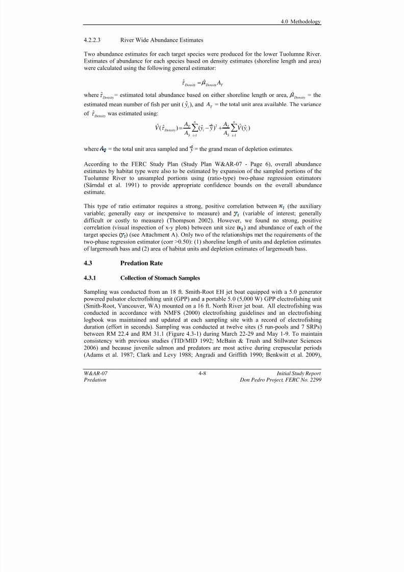
4.2.2.3 River Wide Abundance Estimates
Two abundance estimates for each target species were produced for the lower Tuolumne River.
Estimates of abundance for each species based on density estimates (shoreline length and area)
were calculated using the following general estimator:
Density
Density
AT
where Density
= estimated total abundance based on either shoreline length or area, Density
= the
estimated mean number of fish per unit ( ˆ yi ), and AT
= the total unit area available. The variance
of Density
was estimated using:
V ( Density)AT
AS
(i1
n
ˆ yi ˆ y )2
AT
AS
V (i1
n
ˆ yi )
where = the total unit area sampled and ˆ y = the grand mean of depletion estimates.
According to the FERC Study Plan (Study Plan W&AR-07 - Page 6), overall abundance
estimates by habitat type were also to be estimated by expansion of the sampled portions of theTuolumne River to unsampled portions using (ratio-type) two-phase regression estimators
(Särndal et al. 1991) to provide appropriate confidence bounds on the overall abundance
estimate.
This type of ratio estimator requires a strong, positive correlation between (the auxiliary
variable; generally easy or inexpensive to measure) and (variable of interest; generally
difficult or costly to measure) (Thompson 2002). However, we found no strong, positive
correlation (visual inspection of x-y plots) between unit size ( ) and abundance of each of the
target species ( ) (see Attachment A). Only two of the relationships met the requirements of the
two-phase regression estimator (corr >0.50): (1) shoreline length of units and depletion estimates
of largemouth bass and (2) area of habitat units and depletion estimates of largemouth bass.
4.3 Predation Rate
4.3.1 Collection of Stomach Samples
Sampling was conducted from an 18 ft. Smith-Root EH jet boat equipped with a 5.0 generator
powered pulsator electrofishing unit (GPP) and a portable 5.0 (5,000 W) GPP electrofishing unit
(Smith-Root, Vancouver, WA) mounted on a 16 ft. North River jet boat. All electrofishing wasconducted in accordance with NMFS (2000) electrofishing guidelines and an electrofishing
logbook was maintained and updated at each sampling site with a record of electrofishing
duration (effort in seconds). Sampling was conducted at twelve sites (5 run-pools and 7 SRPs) between RM 22.4 and RM 31.1 (Figure 4.3-1) during March 22-29 and May 1-9. To maintain
consistency with previous studies (TID/MID 1992; McBain & Trush and Stillwater Sciences
2006) and because juvenile salmon and predators are most active during crepuscular periods(Adams et al. 1987; Clark and Levy 1988; Angradi and Griffith 1990; Benkwitt et al. 2009),

7/29/2019 2013 Predation Study on the Don Pedro Project
http://slidepdf.com/reader/full/2013-predation-study-on-the-don-pedro-project 27/71
4.0 Methodology
W&AR-07 4-9 Initial Study Report
Predation Don Pedro Project, FERC No. 2299
sampling began after dark to increase the likelihood that prey in predator stomachs would be
freshly consumed.
Prey items were collected from piscivorous fish, specifically largemouth bass, smallmouth bass,
striped bass and Sacramento pikeminnow > 150 mm FL by inserting an acrylic tube through the
esophagus into the stomach and flushing the stomach with water to disgorge the contents (VanDen Avyle and Roussel 1980; Kamler and Pope 2001). Stomach contents from target species
(noted above) < 150 mm FL were not collected as predation on juvenile salmonids by predators
of this size class has not been observed (TID/MID 1992). Stomach contents were placed in plastic vials and preserved in 70 percent ethanol. The vials were labeled with site, date, and a
unique identification number for each individual sampled.
4.3.2 Identification of Prey Items
In the laboratory, all identifiable prey items found in predator stomachs were classified to order and for fish prey, to genus and species. All intact prey items were measured to the nearest
millimeter (mm). Standard lengths (SL), fork lengths (FL), and total lengths (TL) of fish weretaken when possible. All identifiable prey items, regardless of taxon, were enumerated.
Observations of prey items such as amphibians or reptiles were also recorded.
Hard parts from digested fish (e.g. cleithra and dentaries) were used to help identify fish to genus
and when possible, were measured to estimate the original prey length. Diagnostic bones fromChinook salmon were identified using bone keys developed by Hansel et al. (1988) and Frost
(2000). The diagnostic bones only allow identification to genus (e.g. presence of a cleithrum
would allow identification of presence of Oncorhynchus spp. but not allow distinction betweenO. tshawyscha or O. mykiss). Despite this limitation, we feel justified in calling all cleithrum
identified as Oncorhynchus spp. as belonging to juvenile Chinook salmon because: (1) of the 30identifiable Oncorhynchus spp., all were identified as juvenile Chinook, and (2) only one
juvenile O. mykiss was captured during rotary screw trap monitoring conducted at RM 29.8 near
Waterford. Nearly all (>99.9 percent) salmonid captures in the Waterford rotary screw trapduring spring 2012 were juvenile Chinook salmon (Sonke and Fuller 2012). The presence of
cleithra and dentaries from juvenile Chinook salmon within a particular stomach sample allowed
for the identification of highly digested prey items. To aid in the identification of the diagnostic
bones from stomach samples, we dissected juvenile Chinook (mortalities from other monitoring programs). The cleithra and dentaries from known Chinook were placed in vials for future
reference.

7/29/2019 2013 Predation Study on the Don Pedro Project
http://slidepdf.com/reader/full/2013-predation-study-on-the-don-pedro-project 28/71
W&AR-07 4-10
Predation Do
Figure 4.3-1. Predation rate sampling sites.

7/29/2019 2013 Predation Study on the Don Pedro Project
http://slidepdf.com/reader/full/2013-predation-study-on-the-don-pedro-project 29/71
4.0 Methodology
W&AR-07 4-11 Initial Study Report
Predation Don Pedro Project, FERC No. 2299
4.3.3 Data Analysis
4.3.3.1 Water Temperatures Prior to Time of Capture
Water temperature data from 18 h prior to capture was summarized for each captured predator
based on capture time and location (refer to section 4.3.3.2 for further explanation). Four temperature recorders (Tuolumne Weir, SRP10, Waterford, and Hickman Bridge) were located
within the reach sampled. Based on geographic proximity, sampling locations at Santa Fe,
Hughson, Below Tuolumne Weir, Above Tuolumne Weir, and Charles Road used temperaturereadings from the temperature recorder located at the Tuolumne Weir. Other temperature
recorders and associated sampling locations are described in Table 4.3-1. The mean, standard
deviation, minimum, and maximum water temperature values were calculated using data fromthe temperature recorder nearest the capture location of each predator. The minimum and
maximum temperatures for any given sampling location and period were used to determine
“global” temperature values for the calculation of the gastric evacuation rates.
Table 4.3-1. Location information of temperature recorders and predation rate sampling
locations on the lower Tuolumne River during Spring and Summer 2012.
Temperature
Recorder Site
River
MileAssociated Sampling Sites
Tuolumne Weir 24.4Santa Fe, Hughson, Below Tuolumne Weir, Above Tuolumne Weir, andCharles Road
SRP10 25.5 SRP10 and SRP9
Waterford 29.8 SRP8, lower SRP7, and upper SRP7
Hickman Bridge 31.6 Waterford Wastewater Facility
4.3.3.2 Gastric Evacuation Rates
Gastric evacuation rates, the time it takes for food items to be digested, of fish is largelydetermined by water temperature. Generally, gastric evacuation rates are higher when water temperature is higher, and conversely, rates are lower when water temperatures are lower.
Gastric evacuation rates used for this study were adapted from rates used by TID/MID (1992) based on differences in temperature between the 1992 study and this study. The 1992 study used
10-15 hours for a juvenile Chinook salmon to become unrecognizable at approximately 17°C.
Since gastric evacuation rates are slower at cooler temperatures and water temperatures were
cooler during 2012 (13-18°C), using the same gastric evacuation rates could inflate estimated predation rates. To adjust for the difference in temperature, gastric evacuation rates of 16 hours
and 20 hours were used for this study. Both times were chosen to provide lower and upper
estimates of predation rates, similar to the approach used TID/MID study (1992).
4.3.3.3 Predation Ratio and Predation Rates
Predation ratios, or the average number of juvenile Chinook salmon consumed per predator
sampled, were calculated for each species, sampling event and habitat type (run-pool or specialrun-pool). For example, during the first sampling event in run-pools, 19 largemouth bass were
sampled. The total number of salmon consumed by those 19 largemouth bass was one, which

7/29/2019 2013 Predation Study on the Don Pedro Project
http://slidepdf.com/reader/full/2013-predation-study-on-the-don-pedro-project 30/71
4.0 Methodology
W&AR-07 4-12 Initial Study Report
Predation Don Pedro Project, FERC No. 2299
leads to a predation ratio of 1/19 = 0.053. Confidence intervals for predation ratios were
estimated using a normal approximation to the Poisson distribution using the “epitools” packageand the software R.2.14.1 (Aragon 2010; R Development Core Team 2010).
Predation rates were then calculated using the gastric evacuation times and predation ratios for
each species, sampling event, and habitat type. Using the example from above, the predationratio for largemouth bass in run-pools during the first sampling event was 0.053 juvenile
Chinook consumed per predator. The predation rate at the high digestion rate (using 16 h or
0.667 d) would be equal to 0.053 / 0.667 which is 0.08 juvenile Chinook salmon consumed per largemouth bass per day in run-pool habitats during the first sampling event.
To determine if predation rates were different between sampling events and habitat types, thenumber of predators that consumed salmon was divided by the total number of predators
captured (by species, habitat type and event). To determine if the proportions were different, a
two-sample test for equality of proportions with continuity correction was conducted (Crawley2007). All tests were conducted at α = 0.05.
4.4 Predator Movement Tracking
4.4.1 Acoustic Tag System Overview
Fish movements were monitored with an acoustic tracking system. The project incorporated an
HTI Acoustic Tag Tracking System (ATS), which uses a fixed array of underwater hydrophones
to track movements of fish implanted with acoustic tags. As fish approached the array, the
transmitted signal from each tag was detected and the arrival time recorded at severalhydrophones. The difference in tag signal times at each hydrophone were used to calculate a
two-dimensional (2-D) position.
All tags used in this study operated at 307 kilohertz (kHz) frequency and were encapsulated with
a non-reactive, inert, low toxicity resin compound. The tags utilized “pulse-rate encoding”
which provided increased detection range, improved the signal-to-noise ratio and pulse-arrivalresolution, and decreased position variability when compared to other types of acoustic tags
(Ehrenberg and Steig 2003). Pulse-rate encoding uses the interval between each transmission to
detect and identify the tag. Each tag was programmed with a unique pulse-rate to track movements of individual tagged fish.
The pulse-rate is measured from the leading edge of one pulse to the leading edge of the next
pulse in sequence. By using slightly different pulse-rates, tags can be individually identified.
The timing of the start of each transmission is precisely controlled by a microprocessor withinthe tag. Each tag was programmed to have its own tag period to uniquely identify between tags.
Test tag periods ranged between 2.007 and 4.086 seconds. The amount of time that the tagactively transmits is the pulse length. For this study, the transmit pulse length was 3.0
milliseconds.
In addition to the tag period, the HTI tag subcode option can be used to increase the number of
unique tag ID codes available. Using this tag coding option, each tag is programmed with a
7/29/2019 2013 Predation Study on the Don Pedro Project
http://slidepdf.com/reader/full/2013-predation-study-on-the-don-pedro-project 31/71
4.0 Methodology
W&AR-07 4-13 Initial Study Report
Predation Don Pedro Project, FERC No. 2299
defined primary tag period, and also with a defined secondary transmit signal, called the
subcode. This subcode defines a precise elapsed time period between the primary and secondarytag transmissions. Two subcodes were used for this study; with subcode 8 used for predators,
and subcode 5 for Chinook.
4.4.2
Predator Tagging
Hook and line (angling) surveys as well as electrofishing were conducted between April 26 and
May 16, 2012, with the objective of capturing potential salmonid predators (largemouth bass,smallmouth bass, striped bass, and Sacramento pikeminnow) >150 mm total length.
Sampling was conducted at SRP 6 (RM 30.3), SRP 10 (RM 25.4), Riffle 62 (RM 30.2), andRiffle 74 (RM 24.9) (Figure 4.4-1), as well as areas near these sites where habitat conditions
appeared to be suitable for predators. Light- and medium-weight spinning rod and reel
combinations with monofilament 8-20 lb test fishing lines were used during sampling. Anglersused lures meant to mimic prey fish 60-150 mm in length, and fished from the surface down to
the river bottom. Additional tagging was conducted opportunistically of predators captured byelectrofishing as part of the predation rate sampling.
All predators captured were placed in holding containers with fresh river water. Fish were not
anesthetized with tricaine methanesulfonate due to possible issues if released fish are
subsequently captured and consumed by humans, and no other anesthetizing agents were used.Prior to tagging, fork length (nearest mm) and weight (nearest 0.1 g) were recorded for each fish.
Non-biological data was also recorded including the time and location (GPS coordinates) of
capture, specific habitat type at capture site, and general physical conditions (i.e., weather conditions, water temperature, turbidity, conductivity, and dissolved oxygen).
Predatory fish larger than 150 mm were tagged with an acoustic tag. All tagging was conducted
near the original site of capture. Tags were placed externally and consisted of an HTI
(Hydroacoustic Technology, Inc., Seattle WA) acoustic tag (LG-type) affixed directly under thedorsal fin. Acoustic tags were programmed just before entering the field. Tags were
programmed with a three millisecond pulse width, and tag periods ranging from 2007–4086
milliseconds. At these settings, the predicted tag lives were 40–50 days. During the tagging
process, fish were held in a canvas sling and submerged in running water to keep them calm. Theacoustic tag, mounted to a thin rubber plate with a nylon coated wire leader, was attached by
passing the wires through the body of the fish under the dorsal fin using hypodermic syringe
needles. The wires and tag were secured in place by wire connector sleeves. A t-anchor Floy tag(Floy Tag Inc, Seattle, WA) was also attached directly below the posterior portion of the dorsal
fin. Each Floy tag had unique ID and contact information for anglers to return tags from any
captured fish. This tagging procedure is comparable to that used by California Department of Water Resources (CDWR) staff in the Delta for similar tracking studies.
Tagged fish were allowed to recover in a live well and released back into the river near theoriginal site of capture. During the recovery period, tagged fish were monitored to confirm the
operational status of each transmitter. Fish not selected for tagging were released immediately

7/29/2019 2013 Predation Study on the Don Pedro Project
http://slidepdf.com/reader/full/2013-predation-study-on-the-don-pedro-project 32/71
4.0 Methodology
W&AR-07 4-14 Initial Study Report
Predation Don Pedro Project, FERC No. 2299
after necessary biological data was collected. All fish were acclimated to river conditions prior to
release.
4.4.3 Chinook Salmon Releases
Acoustic tags were surgically implanted into 222 coded wire tagged Chinook salmon provided by CDFG from the Merced River Hatchery (MRH). An additional 600 coded wire tagged
Chinook salmon, also provided from MRH, were marked photonically and were released to
accompany the acoustic tagged fish. All tagging and marking was conducted at MRH.
4.4.3.1 Acoustic Tagging of Chinook Salmon
Acoustic tags were soaked for at least 24 hours prior to programming, and each tag was
programmed with a unique code the day prior to tagging. After programming, tags were sniffed
in a cup of water using a HTI sniffer and monitored through at least three transmission cycles. Atleast five attempts were made to program each tag. Function and coding of all activated tags was
verified with a hydrophone immediately after programming and prior to surgical implantation instudy fish to confirm tag function and programming. Only three tags failed to initialize, and all
programmed tags were heard during validation immediately after programming. Tags wereexpected to remain active for 10-16 days after programming.
During each tagging session, fish were surgically implanted with HTI Model 795 Lm microacoustic tags following implantation procedures outlined in Adams et al. 1998 and Martinelli et
al. 1998. These tags weighed 0.63 g to 0.70 g, and were 16.4 mm long with a diameter of 6.7
mm. Prior to transmitter implantation, fish were anesthetized in 70 mg/L tricainemethanesulfonate buffered with an equal concentration of sodium bicarbonate until they lost
equilibrium. Fish were removed from anesthesia, and were measured (FL to nearest mm) andweighed (to nearest 0.1 g), fish were surgically implanted with acoustic transmitters. Typical
surgery times were less than 3 min.

7/29/2019 2013 Predation Study on the Don Pedro Project
http://slidepdf.com/reader/full/2013-predation-study-on-the-don-pedro-project 33/71
W&AR-07 4-15
Predation Do
Figure 4.4-1. Acoustic array deployment locations.

7/29/2019 2013 Predation Study on the Don Pedro Project
http://slidepdf.com/reader/full/2013-predation-study-on-the-don-pedro-project 34/71
4.0 Methodology
W&AR-07 4-16 Initial Study Report
Predation Don Pedro Project, FERC No. 2299
Fish were then placed into perforated 19 L buckets in a tank inside the egg building at MRH to
recover from anesthesia effects. Buckets were perforated, starting 15 cm from the bottom, toallow water exchange. The non-perforated section of the bucket held 7 L of water to allow
transfer without complete dewatering and without the need to net fish, thereby reducing stress.
Each bucket was stocked with up to three tagged fish, and was covered with a snap-on lid.
In order to evaluate the effects of tagging and transport, 12 Chinook salmon were implanted with
inactive transmitters during each tagging session. Inactive tags were interspersed randomly into
the tagging order for each release group. Procedures for tagging these fish, transporting them tothe release site, and holding them at the release site were the same as for fish with active
transmitters. Dummy-tagged fish were evaluated for condition (i.e., percent scale loss, body
color, fin hemorrhaging, eye quality, and gill coloration) and mortality after being held at therelease site for approximately 40-60 hours.
4.4.3.2 Photonic Marking of Chinook Salmon
A photonic marking system was used for marking fish to accompany the acoustic tagged fish. Allfish were anesthetized with tricaine methanesulfonate before marking. A marker tip was placed
against the anal fin and orange photonic dye was injected into the fin rays. The photonic dye(DayGlo Color Corporation, Cleveland, OH) was chosen because of its known ability to provide
a highly visible, long-lasting mark.
4.4.3.3 Transport and Holding of Chinook Salmon
Once each tagging session was complete, buckets containing acoustic tagged Chinook salmonwere transferred to a dual chambered 250 gallon insulated aluminum hauling tank for transport to
the release site at Hickman Bridge (RM 31.6). At the release site acoustic tagged Chinook salmon were transferred from the buckets to perforated 32 gallon trash cans suspended in the
river in an area of low velocity along the south bank under the bridge. A total of 18-21 Chinook
salmon were transferred to each of the four perforated trash cans.
Photonic marked Chinook salmon were netted from the transport tank and carried in buckets to
live cars suspended in the river adjacent to the trash cans holding the acoustic tagged Chinook
salmon. An in-river holding period prior to release provided time for study fish to recover fromsurgery and transport, and to adjust to in-river water quality for approximately 30-60 hours. Prior
to release, tagged fish were monitored by hydrophones to confirm the operational status of each
tag. All tags were confirmed to be functional during this evaluation.
4.4.3.4 Releases of Tagged and Marked Chinook Salmon
Releases of tagged and marked Chinook salmon were made on May 9-10, May 16-17, and May
21-22, and were timed to occur at flows of 2100 cfs, 280 cfs, and 415 cfs (Table 4.4-1). Each of
the three releases groups of 73-75 acoustic tagged Chinook salmon was paired with a release 200 photonic marked Chinook salmon. To account for potential diurnal differences in Chinook
salmon and predator behavior, approximately half of each group was released shortly before
dawn and half shortly before dusk to allow observation of movement during day and night.
7/29/2019 2013 Predation Study on the Don Pedro Project
http://slidepdf.com/reader/full/2013-predation-study-on-the-don-pedro-project 35/71
4.0 Methodology
W&AR-07 4-17 Initial Study Report
Predation Don Pedro Project, FERC No. 2299
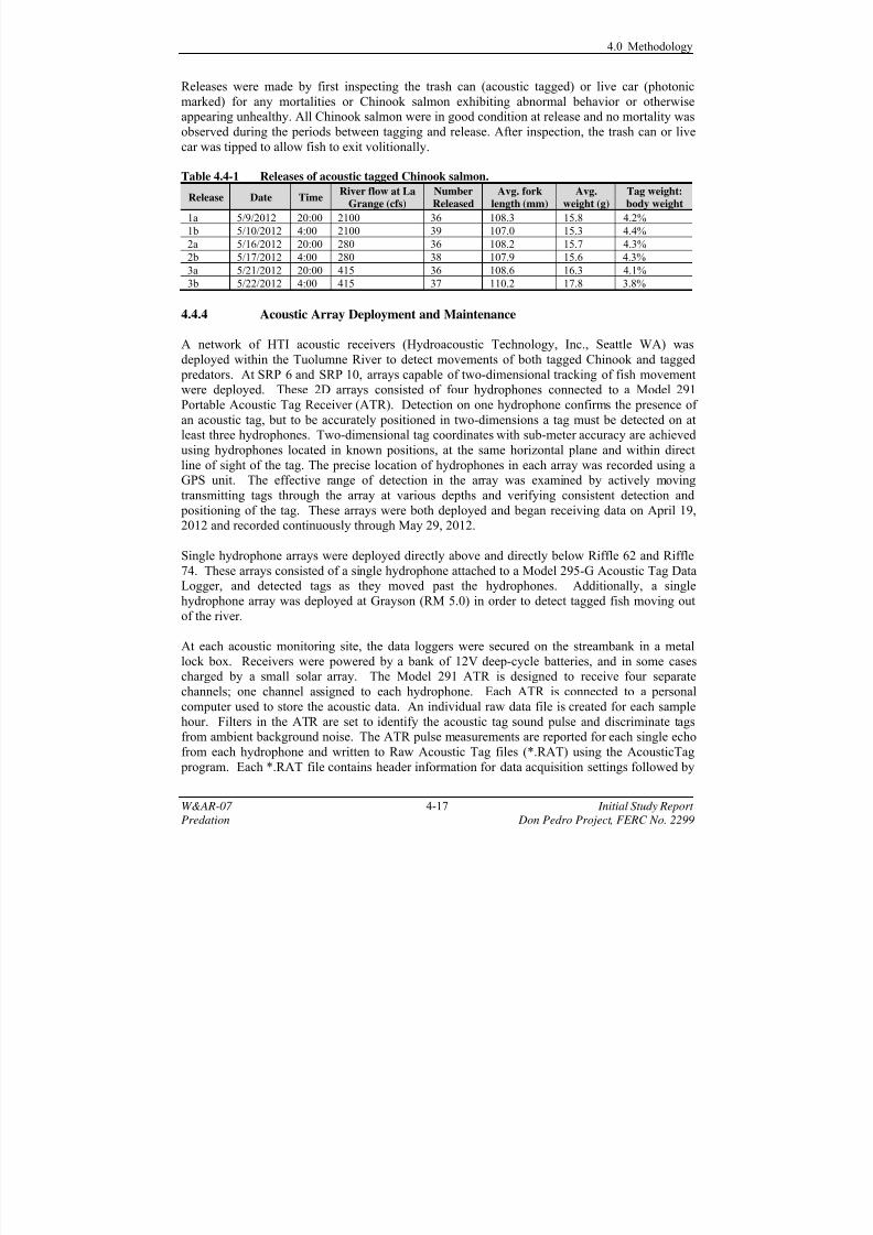
Releases were made by first inspecting the trash can (acoustic tagged) or live car (photonic
marked) for any mortalities or Chinook salmon exhibiting abnormal behavior or otherwiseappearing unhealthy. All Chinook salmon were in good condition at release and no mortality was
observed during the periods between tagging and release. After inspection, the trash can or live
car was tipped to allow fish to exit volitionally.
Table 4.4-1 Releases of acoustic tagged Chinook salmon.
4.4.4 Acoustic Array Deployment and Maintenance
A network of HTI acoustic receivers (Hydroacoustic Technology, Inc., Seattle WA) was
deployed within the Tuolumne River to detect movements of both tagged Chinook and tagged
predators. At SRP 6 and SRP 10, arrays capable of two-dimensional tracking of fish movementwere deployed. These 2D arrays consisted of four hydrophones connected to a Model 291
Portable Acoustic Tag Receiver (ATR). Detection on one hydrophone confirms the presence of
an acoustic tag, but to be accurately positioned in two-dimensions a tag must be detected on atleast three hydrophones. Two-dimensional tag coordinates with sub-meter accuracy are achieved
using hydrophones located in known positions, at the same horizontal plane and within direct
line of sight of the tag. The precise location of hydrophones in each array was recorded using aGPS unit. The effective range of detection in the array was examined by actively moving
transmitting tags through the array at various depths and verifying consistent detection and positioning of the tag. These arrays were both deployed and began receiving data on April 19,2012 and recorded continuously through May 29, 2012.
Single hydrophone arrays were deployed directly above and directly below Riffle 62 and Riffle
74. These arrays consisted of a single hydrophone attached to a Model 295-G Acoustic Tag DataLogger, and detected tags as they moved past the hydrophones. Additionally, a single
hydrophone array was deployed at Grayson (RM 5.0) in order to detect tagged fish moving out
of the river.
At each acoustic monitoring site, the data loggers were secured on the streambank in a metal
lock box. Receivers were powered by a bank of 12V deep-cycle batteries, and in some casescharged by a small solar array. The Model 291 ATR is designed to receive four separate
channels; one channel assigned to each hydrophone. Each ATR is connected to a personal
computer used to store the acoustic data. An individual raw data file is created for each sample
hour. Filters in the ATR are set to identify the acoustic tag sound pulse and discriminate tagsfrom ambient background noise. The ATR pulse measurements are reported for each single echo
from each hydrophone and written to Raw Acoustic Tag files (*.RAT) using the AcousticTag
program. Each *.RAT file contains header information for data acquisition settings followed by
Release Date TimeRiver flow at La
Grange (cfs)
Number
Released
Avg. fork
length (mm)
Avg.
weight (g)
Tag weight:
body weight
1a 5/9/2012 20:00 2100 36 108.3 15.8 4.2%
1b 5/10/2012 4:00 2100 39 107.0 15.3 4.4%
2a 5/16/2012 20:00 280 36 108.2 15.7 4.3%
2b 5/17/2012 4:00 280 38 107.9 15.6 4.3%
3a 5/21/2012 20:00 415 36 108.6 16.3 4.1%
3b 5/22/2012 4:00 415 37 110.2 17.8 3.8%
7/29/2019 2013 Predation Study on the Don Pedro Project
http://slidepdf.com/reader/full/2013-predation-study-on-the-don-pedro-project 36/71
4.0 Methodology
W&AR-07 4-18 Initial Study Report
Predation Don Pedro Project, FERC No. 2299
the raw echo data. Each raw echo data file contains all acoustic signals detected during the time
period, including signals from tagged fish as well as some additional unfiltered acoustic noise.Receiver sites were visited a minimum of three days per week during the acoustic monitoring
period. On each visit, acoustic data was saved to a USB drive and the 12V batteries were
replaced as needed.
At the end of the monitoring period, all acoustic data were auto-marked using HTI’s MarkTags
software. After the data were marked, the files from the SRP6 and SRP 10 arrays were were
geo-referenced and given 2D positions by HTI staff using AcousticTag software. The 2D positions were then imported into Eonfusion software (Myriax Software Pty Ltd) to allow for
viewing of all of the acoustic tracks. The data were reviewed in Eonfusion and the fate of each
acoustic tagged Chinook salmon was classified as either a successful passage, likely consumed by a predator, unknown, or not present. Tag fates were determined based on characteristics of
the tag tracks including length of detection, direction of travel, habitat usage (near-shore vs. mid-
channel) and comparison to tracks of known tagged predators. Predator tags were classified byspecies (largemouth bass, smallmouth bass, striped bass, or Sacramento pikeminnow).
Habitat use by tagged predators and Chinook salmon was evaluated by measuring the relative
density of acoustic tracks within the 2D arrays at the 90 percentile level. These values were usedto calculate the areas of overlap and non-overlap between the successful Chinook passages and
the various predator species using the Eonfusion software package.

7/29/2019 2013 Predation Study on the Don Pedro Project
http://slidepdf.com/reader/full/2013-predation-study-on-the-don-pedro-project 37/71
W&AR-07 5-1 Initial Study Report
Predation Don Pedro Project, FERC No. 2299
5.0 RESULTS
5.1 River Conditions
Flows during the study period ranged from 94 cfs to 2120 cfs (Figure 5.1-1). Predator
abundance sampling was conducted July 25 to August 8, 2012 at an average flow of 98 cfs.Predation rate sampling was conducted on two occasions: March 22 to March 29 and May 1 to
May 9, 2012. During the first sampling period flows were steady at 315 cfs. The second
sampling event occurred on the front end of a pulse flow, with releases ranging from 667 cfs to
2120 cfs. Predator tracking occurred from April 19 to May 29, 2012, with flows ranging from195 cfs to 2120 cfs.
Figure 5.1-2 shows the range of water temperatures between Roberts Ferry Bridge (RM 39.4)and Grayson (RM 5.0) throughout the study period.
Figure 5.1-1. Daily mean discharge at La Grange (LGN) March 1 through August 31 and timing
of sampling events.
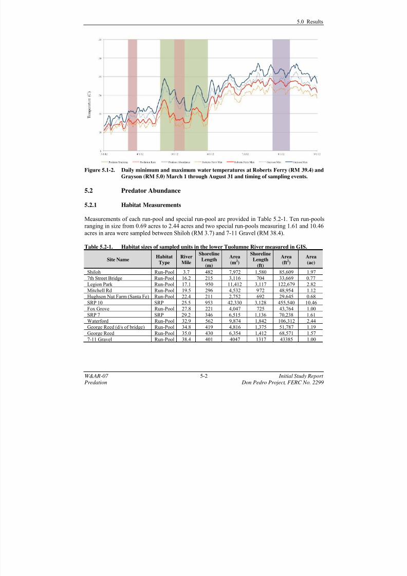
7/29/2019 2013 Predation Study on the Don Pedro Project
http://slidepdf.com/reader/full/2013-predation-study-on-the-don-pedro-project 38/71
5.0 Results
W&AR-07 5-2 Initial Study Report
Predation Don Pedro Project, FERC No. 2299
Figure 5.1-2. Daily minimum and maximum water temperatures at Roberts Ferry (RM 39.4) and
Grayson (RM 5.0) March 1 through August 31 and timing of sampling events.
5.2 Predator Abundance
5.2.1 Habitat Measurements
Measurements of each run-pool and special run-pool are provided in Table 5.2-1. Ten run-poolsranging in size from 0.69 acres to 2.44 acres and two special run-pools measuring 1.61 and 10.46
acres in area were sampled between Shiloh (RM 3.7) and 7-11 Gravel (RM 38.4).
Table 5.2-1. Habitat sizes of sampled units in the lower Tuolumne River measured in GIS.
Site NameHabitat
Type
River
Mile
Shoreline
Length
(m)
Area
(m2)
Shoreline
Length
(ft)
Area
(ft2)
Area
(ac)
Shiloh Run-Pool 3.7 482 7,972 1,580 85,609 1.97
7th Street Bridge Run-Pool 16.2 215 3,116 704 33,669 0.77
Legion Park Run-Pool 17.1 950 11,412 3,117 122,679 2.82
Mitchell Rd Run-Pool 19.5 296 4,532 972 48,954 1.12
Hughson Nut Farm (Santa Fe) Run-Pool 22.4 211 2,752 692 29,645 0.68
SRP 10 SRP 25.5 953 42,330 3,128 455,540 10.46
Fox Grove Run-Pool 27.8 221 4,047 725 43,764 1.00
SRP 7 SRP 29.2 346 6,515 1,136 70,238 1.61
Waterford Run-Pool 32.9 562 9,874 1,842 106,312 2.44
George Reed (d/s of bridge) Run-Pool 34.8 419 4,816 1,375 51,787 1.19
George Reed Run-Pool 35.0 430 6,354 1,412 68,571 1.57
7-11 Gravel Run-Pool 38.4 401 4047 1317 43385 1.00
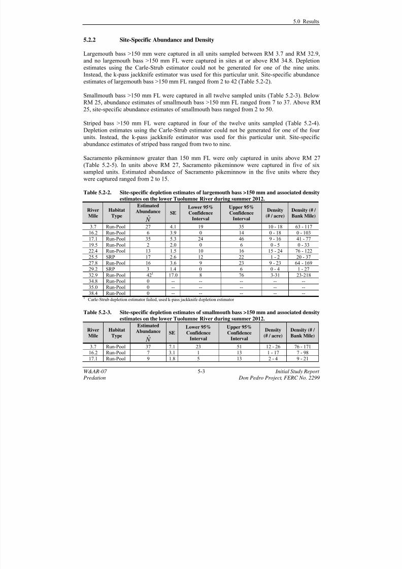
7/29/2019 2013 Predation Study on the Don Pedro Project
http://slidepdf.com/reader/full/2013-predation-study-on-the-don-pedro-project 39/71
5.0 Results
W&AR-07 5-3 Initial Study Report
Predation Don Pedro Project, FERC No. 2299
5.2.2 Site-Specific Abundance and Density
Largemouth bass >150 mm were captured in all units sampled between RM 3.7 and RM 32.9,
and no largemouth bass >150 mm FL were captured in sites at or above RM 34.8. Depletion
estimates using the Carle-Strub estimator could not be generated for one of the nine units.
Instead, the k-pass jackknife estimator was used for this particular unit. Site-specific abundanceestimates of largemouth bass >150 mm FL ranged from 2 to 42 (Table 5.2-2).
Smallmouth bass >150 mm FL were captured in all twelve sampled units (Table 5.2-3). BelowRM 25, abundance estimates of smallmouth bass >150 mm FL ranged from 7 to 37. Above RM
25, site-specific abundance estimates of smallmouth bass ranged from 2 to 50.
Striped bass >150 mm FL were captured in four of the twelve units sampled (Table 5.2-4).
Depletion estimates using the Carle-Strub estimator could not be generated for one of the four
units. Instead, the k-pass jackknife estimator was used for this particular unit. Site-specificabundance estimates of striped bass ranged from two to nine.
Sacramento pikeminnow greater than 150 mm FL were only captured in units above RM 27
(Table 5.2-5). In units above RM 27, Sacramento pikeminnow were captured in five of sixsampled units. Estimated abundance of Sacramento pikeminnow in the five units where they
were captured ranged from 2 to 15.
Table 5.2-2. Site-specific depletion estimates of largemouth bass >150 mm and associated density
estimates on the lower Tuolumne River during summer 2012.
River
Mile
Habitat
Type
Estimated
Abundance
ˆ N SE
Lower 95%
Confidence
Interval
Upper 95%
Confidence
Interval
Density
(# / acre)
Density (# /
Bank Mile)
3.7 Run-Pool 27 4.1 19 35 10 - 18 63 - 117
16.2 Run-Pool 6 3.9 0 14 0 - 18 0 - 103
17.1 Run-Pool 35 5.3 24 46 9 - 16 41 - 77
19.5 Run-Pool 2 2.0 0 6 0 - 5 0 - 33
22.4 Run-Pool 13 1.5 10 16 15 - 24 76 - 122
25.5 SRP 17 2.6 12 22 1 - 2 20 - 37
27.8 Run-Pool 16 3.6 9 23 9 - 23 64 - 169
29.2 SRP 3 1.4 0 6 0 - 4 1 - 27
32.9 Run-Pool 421 17.0 8 76 3-31 23-218
34.8 Run-Pool 0 -- -- -- -- --
35.0 Run-Pool 0 -- -- -- -- --
38.4 Run-Pool 0 -- -- -- -- --1 Carle-Strub depletion estimator failed, used k-pass jackknife depletion estimator
Table 5.2-3. Site-specific depletion estimates of smallmouth bass >150 mm and associated density
estimates on the lower Tuolumne River during summer 2012.
River
Mile
Habitat
Type
Estimated
Abundance
ˆ N SE
Lower 95%
Confidence
Interval
Upper 95%
Confidence
Interval
Density
(# / acre)
Density (# /
Bank Mile)
3.7 Run-Pool 37 7.1 23 51 12 - 26 76 - 171
16.2 Run-Pool 7 3.1 1 13 1 - 17 7 - 98
17.1 Run-Pool 9 1.8 5 13 2 - 4 9 - 21

7/29/2019 2013 Predation Study on the Don Pedro Project
http://slidepdf.com/reader/full/2013-predation-study-on-the-don-pedro-project 40/71
5.0 Results
W&AR-07 5-4 Initial Study Report
Predation Don Pedro Project, FERC No. 2299
River
Mile
Habitat
Type
Estimated
Abundance
ˆ N SE
Lower 95%
Confidence
Interval
Upper 95%
Confidence
Interval
Density
(# / acre)
Density (# /
Bank Mile)
19.5 Run-Pool 26 5.1 16 36 14 - 32 86 - 197
22.4 Run-Pool 14 1.5 11 17 16 - 25 83 - 130
25.5 SRP 9 5.6 0 20 0 - 2 0 - 34
27.8 Run-Pool 15 1.8 11 19 11 - 19 82 - 136
29.2 SRP 2 2.0 0 6 0 - 4 0 - 28
32.9 Run-Pool 15 1.4 12 18 5 - 7 35 - 51
34.8 Run-Pool 50 7.7 35 65 29 - 55 132 - 251
35.0 Run-Pool 2 2.9 0 8 0 - 5 0 - 29
38.4 Run-Pool 32 1.3 29 35 29 - 35 118 - 139
Table 5.2-4. Site-specific depletion estimates of striped bass >150 mm and associated density
estimates on the lower Tuolumne River during summer 2012.
River
Mile
Habitat
Type
Estimated
Abundance
ˆ N
SE
Lower 95%
Confidence
Interval
Upper 95%
Confidence
Interval
Density
(# / acre)
Density (# /
Bank Mile)
3.7 Run-Pool 9 3.0 3 15 2 - 8 10 - 50
16.2 Run-Pool 0 -- -- -- -- --
17.1 Run-Pool 0 -- -- -- -- --
19.5 Run-Pool 0 -- -- -- -- --
22.4 Run-Pool 0 -- -- -- -- --
25.5 SRP 0 -- -- -- -- --
27.8 Run-Pool 4 1.5 1 7 1 - 7 7 - 51
29.2 SRP 0 -- -- -- -- --
32.9 Run-Pool 0 -- -- -- -- --
34.8 Run-Pool 41 0 4 4 3-3 15-15
35.0 Run-Pool 2 5.5 0 13 0 - 8 0 - 48
38.4 Run-Pool 0 -- -- -- -- --1
Carle-Strub depletion estimate failed, used k-pass jackknife depletion estimator.
Table 5.2-5. Site-specific depletion estimates of Sacramento pikeminnow >150 mm and
associated density estimates on the lower Tuolumne River during summer 2012.
River
Mile
Habitat
Type
Estimated
Abundance
ˆ N SE
Lower 95%
Confidence
Interval
Upper 95%
Confidence
Interval
Density
(# / acre)
Density (# /
Bank Mile)
3.7 Run-Pool 0 -- -- -- -- --
16.2 Run-Pool 0 -- -- -- -- --
17.1 Run-Pool 0 -- -- -- -- --
19.5 Run-Pool 0 -- -- -- -- --
22.4 Run-Pool 0 -- -- -- -- --
25.5 SRP 0 -- -- -- -- --27.8 Run-Pool 2 2.9 0 8 0 - 8 0 - 57
29.2 SRP 0 -- -- -- -- --
32.9 Run-Pool 15 1.8 11 19 5 - 8 32 - 54
34.8 Run-Pool 3 3.5 0 10 0 - 8 0 - 38
35.0 Run-Pool 12 4.0 4 20 2 - 13 15 - 75
38.4 Run-Pool 12 1.8 8 16 8 - 16 34 - 62

7/29/2019 2013 Predation Study on the Don Pedro Project
http://slidepdf.com/reader/full/2013-predation-study-on-the-don-pedro-project 41/71
5.0 Results
W&AR-07 5-5 Initial Study Report
Predation Don Pedro Project, FERC No. 2299
5.2.3 River Wide Abundance Estimates
Correlation values between habitat size (shoreline lengths and habitat areas) and site-specific
abundance estimates were low and ranged from .033 to .606 (Attachment A). With the exception
of largemouth bass, all correlations between habitat size and predator abundance estimates failed
to meet the minimum suggested level of 0.5 to use a ratio-regression estimator (Thompson 2002;Hankin, unpublished); therefore the ratio-regression estimator could not be used to generate
river-wide abundance estimates.
Two abundance estimates for each species were produced for the lower Tuolumne River. The
first is based on areal density and the second is based on shoreline density (Table 5.2-6). River
wide abundance estimates (for all run-pools and special run-pools from RM 0 to RM 39.4)derived from area density estimates were slightly higher than those derived from shoreline
density estimates. Smallmouth bass were estimated to be the most abundant predators, with
9,092 and 6,764 based on area and shoreline length, respectively. A standard error term could not be produced for either of the striped bass estimates since depletion was not achieved at RM 34.8.
Table 5.2-6. Abundance estimates and associated standard errors based on estimated densities
(by area and shoreline length of run-pools and special run-pools) of each target
species on the lower Tuolumne River (RM 0 to RM 39.4).
5.3 Predation Rate
A total of 295 piscivores > 150 mm FL were captured during the two sampling occasions. The
first sampling occasion took place from March 22, 2012 to March 29, 2012 and the secondsampling took place from May 1, 2012 to May 9, 2012. No further sampling to estimate
predation rates was conducted after May 9, 2012. Smallmouth and largemouth bass were the
most common piscivores collected. A total of 49 piscivores had no food contents in their
stomach when examined. Similar numbers of empty stomachs were observed for smallmouth bass (15.2 percent) and largemouth bass (14.5 percent). About 35 percent of striped bass sampled
(9 of 26) had empty stomachs when examined (Table 5.3-1).
SpeciesArea
SE
Bass < 150 mm 121,756 4,360
Largemouth bass 4,794 252
Sacramento pikeminnow 1,590 98
Smallmouth bass 9,092 251
Striped bass 692 55
SpeciesShoreline Length
Bass < 150 mm 95,198 4,506
Largemouth bass 4,185 261
Sacramento pikeminnow 1,161 101
Smallmouth bass 6,764 260
Striped bass 588 57

7/29/2019 2013 Predation Study on the Don Pedro Project
http://slidepdf.com/reader/full/2013-predation-study-on-the-don-pedro-project 42/71
5.0 Results
W&AR-07 5-6 Initial Study Report
Predation Don Pedro Project, FERC No. 2299
Table 5.3-1. Numbers of predatory fish (> 150 mm FL) stomachs sampled and number and
percentage of predatory fish with empty stomachs during electrofishing on the
lower Tuolumne River during spring 2012.
Species Number Sampled Number EmptyPercentage of Predators
with Empty Stomach
Smallmouth bass 132 20 15.2%
Largemouth bass 131 19 14.5%Striped bass 26 9 34.6%
Sacramento pikeminnow 6 1 16.7%
5.3.1 Diet Composition
At the taxonomic class level, insects (many orders) made up a majority (74 percent) of
identifiable prey items observed in the 246 stomach samples examined. Other notable prey items
included fish (various orders) at approximately 13.5 percent of all identifiable prey items andcrayfish at approximately 4 percent of all identifiable prey items (Figure 5.3-1). All other prey
items combined made up only eight percent of the identifiable prey items observed in the
stomach samples.
The most frequently occurring prey items were macroinvertebrates of the orders Tricoptera and
Ephemeroptera (Figure 5.3-2). Of the 246 stomach samples examined, 100 (41 percent)contained at least one trichopteran (either larvae or adult) and 92 (37 percent) contained at least
one ephemeropteran (larvae or adult). Seventy-nine or about 32 percent of stomach samples
examined contained at least one unidentified fish (no identifiable juvenile Chinook salmon were
included in this count). Crayfish were present in about 26 percent of all stomach samplesexamined. Thirty fish identified as juvenile Chinook salmon occurred in about 12 percent of the
stomach samples.
When identifiable prey items were counted by order, nearly 46 percent were of the order Ephemeroptera (Figure 5.3-3). The second-most frequent prey item by order was Trichoptera (13
percent).
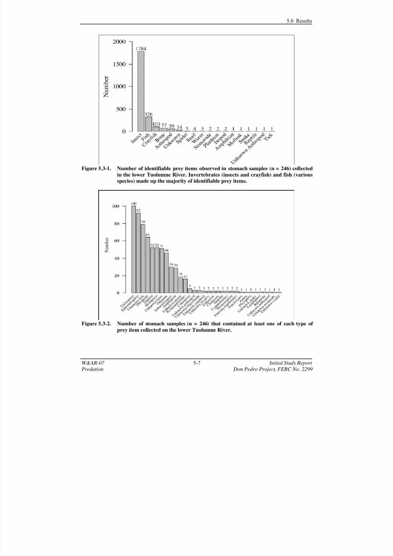
7/29/2019 2013 Predation Study on the Don Pedro Project
http://slidepdf.com/reader/full/2013-predation-study-on-the-don-pedro-project 43/71
5.0 Results
W&AR-07 5-7 Initial Study Report
Predation Don Pedro Project, FERC No. 2299
Figure 5.3-1. Number of identifiable prey items observed in stomach samples (n = 246) collected
in the lower Tuolumne River. Invertebrates (insects and crayfish) and fish (various
species) made up the majority of identifiable prey items.
Figure 5.3-2. Number of stomach samples (n = 246) that contained at least one of each type of
prey item collected on the lower Tuolumne River.

7/29/2019 2013 Predation Study on the Don Pedro Project
http://slidepdf.com/reader/full/2013-predation-study-on-the-don-pedro-project 44/71
5.0 Results
W&AR-07 5-8 Initial Study Report
Predation Don Pedro Project, FERC No. 2299
Figure 5.3-3. Number of prey items (by order) observed in stomach samples (n = 246) collected inthe lower Tuolumne River.
5.3.2 Predation of juvenile Chinook salmon
Of the 246 stomach samples examined, 30 contained juvenile Chinook salmon, with eight of
these samples from smallmouth bass, 11 from largemouth bass, and 11 from striped bass. No
juvenile Chinook salmon were observed in the stomach contents of Sacramento pikeminnow.Smallmouth bass that consumed juvenile Chinook salmon were at least 185 mm FL, largemouth
bass were at least 207 mm FL, and striped bass were at least 180 mm FL (Figure 5.3-4).
During the March sampling event, standard lengths (SL) (measured from snout to hypural plate)
of 13 intact juvenile Chinook salmon found in the stomach contents of sampled predators were
measured. The mean SL was 51.6 mm (sd = 11.0). The smallest observed juvenile Chinook
salmon during the March sampling event was 30 mm SL and the largest was 68 mm SL.
Standard lengths of 14 intact juvenile Chinook salmon were measured from specimens observed
in stomach samples collected during the May sampling event. The mean standard length was71.4 mm (sd = 5.3), about 20 mm larger on average than mean SL observed in the March
sampling event. The smallest observed juvenile Chinook salmon during the May sampling event
was 62 mm SL and the largest was 78 mm SL.
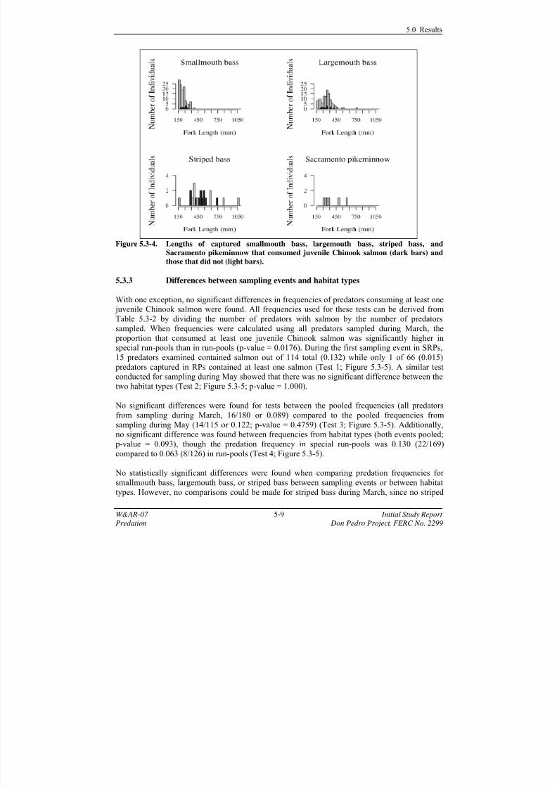
7/29/2019 2013 Predation Study on the Don Pedro Project
http://slidepdf.com/reader/full/2013-predation-study-on-the-don-pedro-project 45/71
5.0 Results
W&AR-07 5-9 Initial Study Report
Predation Don Pedro Project, FERC No. 2299
Figure 5.3-4. Lengths of captured smallmouth bass, largemouth bass, striped bass, and
Sacramento pikeminnow that consumed juvenile Chinook salmon (dark bars) and
those that did not (light bars).
5.3.3 Differences between sampling events and habitat types
With one exception, no significant differences in frequencies of predators consuming at least one juvenile Chinook salmon were found. All frequencies used for these tests can be derived from
Table 5.3-2 by dividing the number of predators with salmon by the number of predatorssampled. When frequencies were calculated using all predators sampled during March, the
proportion that consumed at least one juvenile Chinook salmon was significantly higher inspecial run-pools than in run-pools (p-value = 0.0176). During the first sampling event in SRPs,
15 predators examined contained salmon out of 114 total (0.132) while only 1 of 66 (0.015)
predators captured in RPs contained at least one salmon (Test 1; Figure 5.3-5). A similar testconducted for sampling during May showed that there was no significant difference between the
two habitat types (Test 2; Figure 5.3-5; p-value = 1.000).
No significant differences were found for tests between the pooled frequencies (all predators
from sampling during March, 16/180 or 0.089) compared to the pooled frequencies from
sampling during May (14/115 or 0.122; p-value = 0.4759) (Test 3; Figure 5.3-5). Additionally,no significant difference was found between frequencies from habitat types (both events pooled;
p-value = 0.093), though the predation frequency in special run-pools was 0.130 (22/169)
compared to 0.063 (8/126) in run-pools (Test 4; Figure 5.3-5).
No statistically significant differences were found when comparing predation frequencies for
smallmouth bass, largemouth bass, or striped bass between sampling events or between habitat
types. However, no comparisons could be made for striped bass during March, since no striped
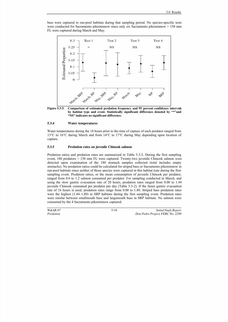
7/29/2019 2013 Predation Study on the Don Pedro Project
http://slidepdf.com/reader/full/2013-predation-study-on-the-don-pedro-project 46/71
5.0 Results
W&AR-07 5-10 Initial Study Report
Predation Don Pedro Project, FERC No. 2299
bass were captured in run-pool habitats during that sampling period. No species-specific tests
were conducted for Sacramento pikeminnow since only six Sacramento pikeminnow > 150 mmFL were captured during March and May.
Figure 5.3-5. Comparison of estimated predation frequency and 95 percent confidence intervalsby habitat type and event. Statistically significant difference denoted by “*”and
“NS” indicates no significant difference.
5.3.4 Water temperatures
Water temperatures during the 18 hours prior to the time of capture of each predator ranged from13°C to 16°C during March and from 14°C to 17°C during May depending upon location of
capture.
5.3.5 Predation rates on juvenile Chinook salmon
Predation ratios and predation rates are summarized in Table 5.3-2. During the first samplingevent, 180 predators > 150 mm FL were captured. Twenty-two juvenile Chinook salmon were
detected upon examination of the 180 stomach samples collected (total includes empty
stomachs). No predation ratios could be calculated for striped bass or Sacramento pikeminnow inrun-pool habitats since neither of those species were captured in this habitat type during the first
sampling event. Predation ratios, or the mean consumption of juvenile Chinook per predator,ranged from 0.0 to 1.2 salmon consumed per predator. For sampling conducted in March, and
using the slow gastric evacuation rate of 20 hours, predation rates ranged from 0.00 to 1.44 juvenile Chinook consumed per predator per day (Table 5.3-2). If the faster gastric evacuation
rate of 16 hours is used, predation rates range from 0.00 to 1.80. Striped bass predation rates
were the highest (1.44–1.80) in SRP habitats during the first sampling event. Predation rateswere similar between smallmouth bass and largemouth bass in SRP habitats. No salmon were
consumed by the 4 Sacramento pikeminnow captured.

7/29/2019 2013 Predation Study on the Don Pedro Project
http://slidepdf.com/reader/full/2013-predation-study-on-the-don-pedro-project 47/71
5.0 Results
W&AR-07 5-11 Initial Study Report
Predation Don Pedro Project, FERC No. 2299
During the second sampling event, 115 predators > 150 mm FL were captured. Twenty-three
juvenile Chinook salmon were detected upon examination of the 115 stomach samples collected(total includes empty stomachs). Predation ratios ranged from 0.0 to 1.0 salmon consumed per
predator. For sampling conducted in May, and using the slow gastric evacuation rate of 20 hours,
predation rates ranged from 0.00 to 1.20 juvenile Chinook consumed per predator per day (Table
5.3-2). With the faster gastric evacuation rate of 16 hours, predation rates ranged from 0.00 to1.50 juvenile Chinook consumed per predator per day. Similar to March, predation rates during
May were highest for striped bass in comparison to the other predator species examined. No
salmon were consumed by the two Sacramento pikeminnow captured.
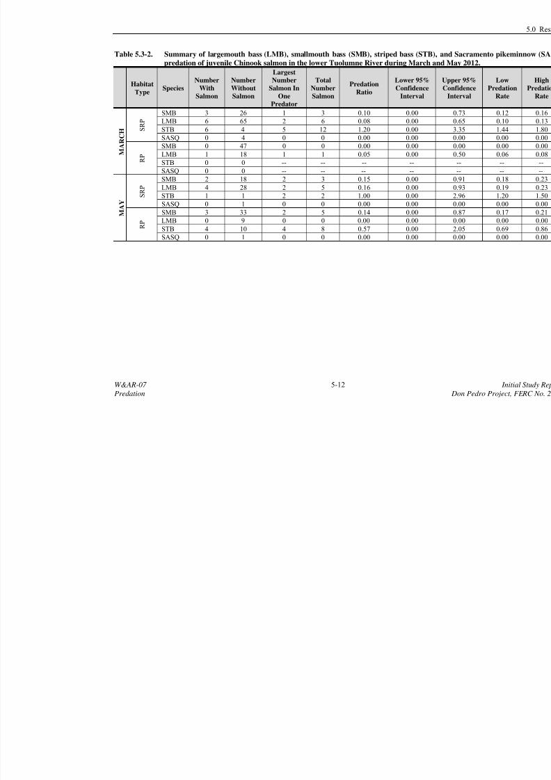
7/29/2019 2013 Predation Study on the Don Pedro Project
http://slidepdf.com/reader/full/2013-predation-study-on-the-don-pedro-project 48/71
W&AR-07 5-12
Predation Do
Table 5.3-2. Summary of largemouth bass (LMB), smallmouth bass (SMB), striped bass (STB), and Sa
predation of juvenile Chinook salmon in the lower Tuolumne River during March and May
Habitat
TypeSpecies
Number
With
Salmon
Number
Without
Salmon
Largest
Number
Salmon In
One
Predator
Total
Number
Salmon
Predation
Ratio
Lower 95%
Confidence
Interval
Upper
Confid
Inter
M A R C H S
R P
SMB 3 26 1 3 0.10 0.00 0.7
LMB 6 65 2 6 0.08 0.00 0.6
STB 6 4 5 12 1.20 0.00 3.3
SASQ 0 4 0 0 0.00 0.00 0.0
R P
SMB 0 47 0 0 0.00 0.00 0.0
LMB 1 18 1 1 0.05 0.00 0.5
STB 0 0 -- -- -- -- --
SASQ 0 0 -- -- -- -- --
M A Y
S R P
SMB 2 18 2 3 0.15 0.00 0.9
LMB 4 28 2 5 0.16 0.00 0.9
STB 1 1 2 2 1.00 0.00 2.9
SASQ 0 1 0 0 0.00 0.00 0.0
R P
SMB 3 33 2 5 0.14 0.00 0.8LMB 0 9 0 0 0.00 0.00 0.0
STB 4 10 4 8 0.57 0.00 2.0
SASQ 0 1 0 0 0.00 0.00 0.0
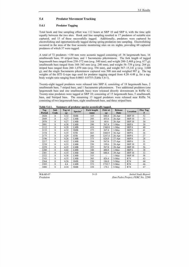
7/29/2019 2013 Predation Study on the Don Pedro Project
http://slidepdf.com/reader/full/2013-predation-study-on-the-don-pedro-project 49/71
5.0 Results
W&AR-07 5-13 Initial Study Report
Predation Don Pedro Project, FERC No. 2299
5.4 Predator Movement Tracking
5.4.1 Predator Tagging
Total hook and line sampling effort was 112 hours at SRP 10 and SRP 6, with the time split
equally between the two sites. Hook and line sampling resulted in 17 predators of suitable sizecaptured, and 15 of these successfully tagged. Additionally, predators were captured byelectrofishing and opportunistically tagged during spring predation rate sampling. Electrofishing
occurred in the area of the four acoustic monitoring sites on six nights, providing 60 captured
predators of which 57 were tagged.
A total of 72 predators >150 mm were acoustic tagged consisting of: 36 largemouth bass, 16
smallmouth bass, 19 striped bass, and 1 Sacramento pikeminnow. The fork length of taggedlargemouth bass ranged from 250–572 mm (avg. 340 mm), and weight 200–2,468 g (avg. 677 g);
smallmouth bass ranged from 168–345 mm (avg. 240 mm), and weight 56–739 g (avg. 264 g);
striped bass ranged from 260–1,070 mm (avg. 556 mm), and weight 567–15,141 g (avg. 3,040
g); and the single Sacramento pikeminnow captured was 508 mm and weighed 907 g. The tagweights of the HTI G-type tags used for predator tagging ranged from 4.20–4.48 g, for a tag-
body weight ratio ranging from 0.0003–0.0755 (Table 5.4-1).
Twenty-eight tagged predators were released into SRP 6; consisting of 18 largemouth bass, 2
smallmouth bass, 7 striped bass, and 1 Sacramento pikeminnow. Two additional predators (one
largemouth bass and one smallmouth bass) were released directly downstream in Riffle 62.Twenty-nine predators were tagged at SRP 10; consisting of 15 largemouth bass, 5 smallmouth
bass, and 9striped bass. The remaining 13 tagged predators were released near Riffle 74;
consisting of two largemouth bass, eight smallmouth bass, and three striped bass.
Table 5.4-1. Summary of predator species acoustically tagged.
Tag
Period
Sub
Code
Tag wt
(g)Species1
Fork length
(mm)
Fish wt
(g)
Release
DateLocation
Floy Tag
#
2028 8 4.32 SMB 325 680.4 26-Apr SRP 10 52
2049 8 4.27 LMB 295 453.6 26-Apr SRP 10 53
2070 8 4.27 LMB 310 68.4 26-Apr SRP 10 54
2091 8 4.38 LMB 290 367.4 1-May SRP 6 39
2112 8 4.28 LMB 410 1360.8 1-May SRP 6 40
2133 8 4.32 SMB 275 367.4 1-May SRP 6 41
2154 8 4.35 STB 665 3460.9 26-Apr SRP 6 26
2175 8 4.29 STB 260 1247.4 26-Apr SRP 6 27
2196 8 4.26 LMB 375 626.0 27-Apr SRP 6 28
2217 8 4.32 LMB 334 567.0 27-Apr SRP 6 31
2238 8 4.33 LMB 250 199.6 28-Apr SRP 10 552259 8 4.35 LMB 325 567.0 28-Apr SRP 10 56
2280 8 4.42 LMB 340 480.8 1-May SRP 6 38
2301 8 4.35 LMB 360 680.4 29-Apr SRP 10 32
2322 8 4.38 LMB 335 -- 1-May SRP 10 58
2343 8 4.35 LMB 305 426.4 5-May R74 63
2364 8 4.26 SMB 230 186.0 5-May R74 64
2385 8 4.4 LMB 572 1732.7 5-May R74 66
2406 8 4.24 SMB 228 170.1 5-May R74 67
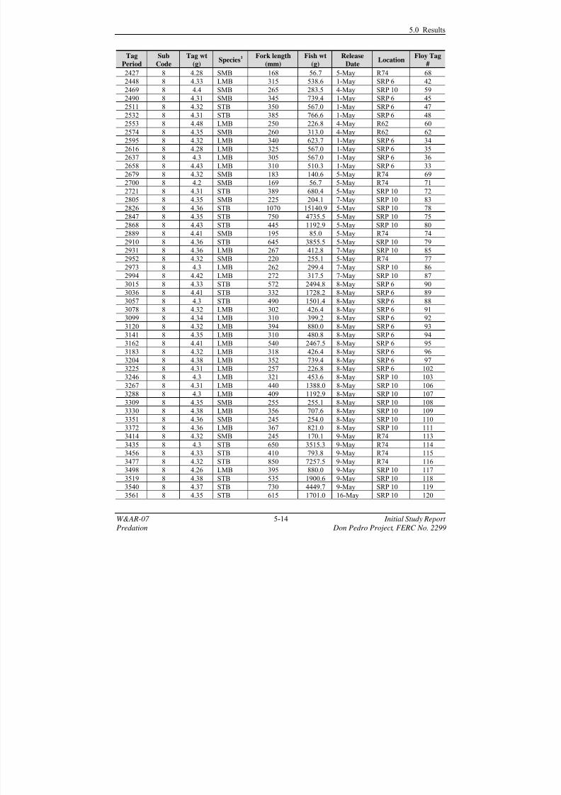
7/29/2019 2013 Predation Study on the Don Pedro Project
http://slidepdf.com/reader/full/2013-predation-study-on-the-don-pedro-project 50/71
5.0 Results
W&AR-07 5-14 Initial Study Report
Predation Don Pedro Project, FERC No. 2299
Tag
Period
Sub
Code
Tag wt
(g)Species1
Fork length
(mm)
Fish wt
(g)
Release
DateLocation
Floy Tag
#
2427 8 4.28 SMB 168 56.7 5-May R74 68
2448 8 4.33 LMB 315 538.6 1-May SRP 6 42
2469 8 4.4 SMB 265 283.5 4-May SRP 10 59
2490 8 4.31 SMB 345 739.4 1-May SRP 6 45
2511 8 4.32 STB 350 567.0 1-May SRP 6 472532 8 4.31 STB 385 766.6 1-May SRP 6 48
2553 8 4.48 LMB 250 226.8 4-May R62 60
2574 8 4.35 SMB 260 313.0 4-May R62 62
2595 8 4.32 LMB 340 623.7 1-May SRP 6 34
2616 8 4.28 LMB 325 567.0 1-May SRP 6 35
2637 8 4.3 LMB 305 567.0 1-May SRP 6 36
2658 8 4.43 LMB 310 510.3 1-May SRP 6 33
2679 8 4.32 SMB 183 140.6 5-May R74 69
2700 8 4.2 SMB 169 56.7 5-May R74 71
2721 8 4.31 STB 389 680.4 5-May SRP 10 72
2805 8 4.35 SMB 225 204.1 7-May SRP 10 83
2826 8 4.36 STB 1070 15140.9 5-May SRP 10 78
2847 8 4.35 STB 750 4735.5 5-May SRP 10 752868 8 4.43 STB 445 1192.9 5-May SRP 10 80
2889 8 4.41 SMB 195 85.0 5-May R74 74
2910 8 4.36 STB 645 3855.5 5-May SRP 10 79
2931 8 4.36 LMB 267 412.8 7-May SRP 10 85
2952 8 4.32 SMB 220 255.1 5-May R74 77
2973 8 4.3 LMB 262 299.4 7-May SRP 10 86
2994 8 4.42 LMB 272 317.5 7-May SRP 10 87
3015 8 4.33 STB 572 2494.8 8-May SRP 6 90
3036 8 4.41 STB 332 1728.2 8-May SRP 6 89
3057 8 4.3 STB 490 1501.4 8-May SRP 6 88
3078 8 4.32 LMB 302 426.4 8-May SRP 6 91
3099 8 4.34 LMB 310 399.2 8-May SRP 6 92
3120 8 4.32 LMB 394 880.0 8-May SRP 6 93
3141 8 4.35 LMB 310 480.8 8-May SRP 6 94
3162 8 4.41 LMB 540 2467.5 8-May SRP 6 95
3183 8 4.32 LMB 318 426.4 8-May SRP 6 96
3204 8 4.38 LMB 352 739.4 8-May SRP 6 97
3225 8 4.31 LMB 257 226.8 8-May SRP 6 102
3246 8 4.3 LMB 321 453.6 8-May SRP 10 103
3267 8 4.31 LMB 440 1388.0 8-May SRP 10 106
3288 8 4.3 LMB 409 1192.9 8-May SRP 10 107
3309 8 4.35 SMB 255 255.1 8-May SRP 10 108
3330 8 4.38 LMB 356 707.6 8-May SRP 10 109
3351 8 4.36 SMB 245 254.0 8-May SRP 10 110
3372 8 4.36 LMB 367 821.0 8-May SRP 10 1113414 8 4.32 SMB 245 170.1 9-May R74 113
3435 8 4.3 STB 650 3515.3 9-May R74 114
3456 8 4.33 STB 410 793.8 9-May R74 115
3477 8 4.32 STB 850 7257.5 9-May R74 116
3498 8 4.26 LMB 395 880.0 9-May SRP 10 117
3519 8 4.38 STB 535 1900.6 9-May SRP 10 118
3540 8 4.37 STB 730 4449.7 9-May SRP 10 119
3561 8 4.35 STB 615 1701.0 16-May SRP 10 120

7/29/2019 2013 Predation Study on the Don Pedro Project
http://slidepdf.com/reader/full/2013-predation-study-on-the-don-pedro-project 51/71
5.0 Results
W&AR-07 5-15 Initial Study Report
Predation Don Pedro Project, FERC No. 2299
Tag
Period
Sub
Code
Tag wt
(g)Species1
Fork length
(mm)
Fish wt
(g)
Release
DateLocation
Floy Tag
#
3582 8 4.33 SASQ 508 907.2 16-May SRP 6 121
3603 8 STB 419 766.6 16-May SRP 10 1221 SMB= smallmouth bass, LMB= largemouth bass, STB= striped bass, SASQ= Sacramento pikeminnow
5.4.2 Detections of Acoustic Tagged Fish
Fate determinations for fish detection in the arrays at SRP 6 and SRP 10 are summarized in
Table 5.4-2. Of the 75 acoustic tagged Chinook salmon released at Hickman Bridge (RM 31.6)on May 9–10 at a flow level of 2,100 cfs, 69 were detected in SRP 6 (RM 30.3). Sixty-three
(91.3 percent) of these successfully passed through SRP 6, two (2.9 percent) were likely
consumed by predators, and the fates of four tags (5.8 percent) were classified as unknown(Table 5.4-2). Travel time from the release site of Chinook that successfully passed through SRP
6 ranged from 0.4 to 9.5 hours (median= 0.5 hours), and duration of detection within SRP 6
ranged from 0.6 to 87.4 minutes (median= 3.7 minutes). The total area covered by tagged
Chinook that successfully passed was 4,546 m2. The overlap of the 90
thpercentile of acoustic
tracks between tagged Chinook and predator species was 8.0 percent for largemouth bass and27.4 percent for striped bass (Figure 5.4-1, Table 5.4-3).
Table 5.4-2. Summary of fate determinations for acoustic tagged Chinook salmon in SRP 6 and
SRP 10, and river flow at La Grange, and water temperature at Roberts Ferry.
Release Group
1 2 3
Release Dates May 9-10 May 16-17 May 21-22
Target Flow at La Grange
(cfs)2,100 280 415
Water Temperature at
Roberts Ferry (°C)12.6 (range: 11.0-14.3) 16.3 (range: 14.6-18.7) 16.7 (range: 13.8-17.1)
Total #Released 75 74 73-- -- --
SRP 6 -- -- --
Detected 69 55 63
Passed 91.3 % (n=63) 54.5% (n=30) 31.7% (n=20)
Consumed 2.9% (n=2) 30.9% (n=17) 60.3% (n=38)
Unknown 5.8% (n=4) 14.5% (n=8) 7.9% (n=5)
-- -- --
SRP 10 -- -- --
Detected 57 22 7
Passed 75.4% (n=43) 50.0% (n=11) 28.6% (n=2)
Consumed 15.8% (n=9) 31.8% (n=7) 71.4% (n=5)
Unknown 8.8% (n=5) 18.2% (n=4) 0.0% (n=0)
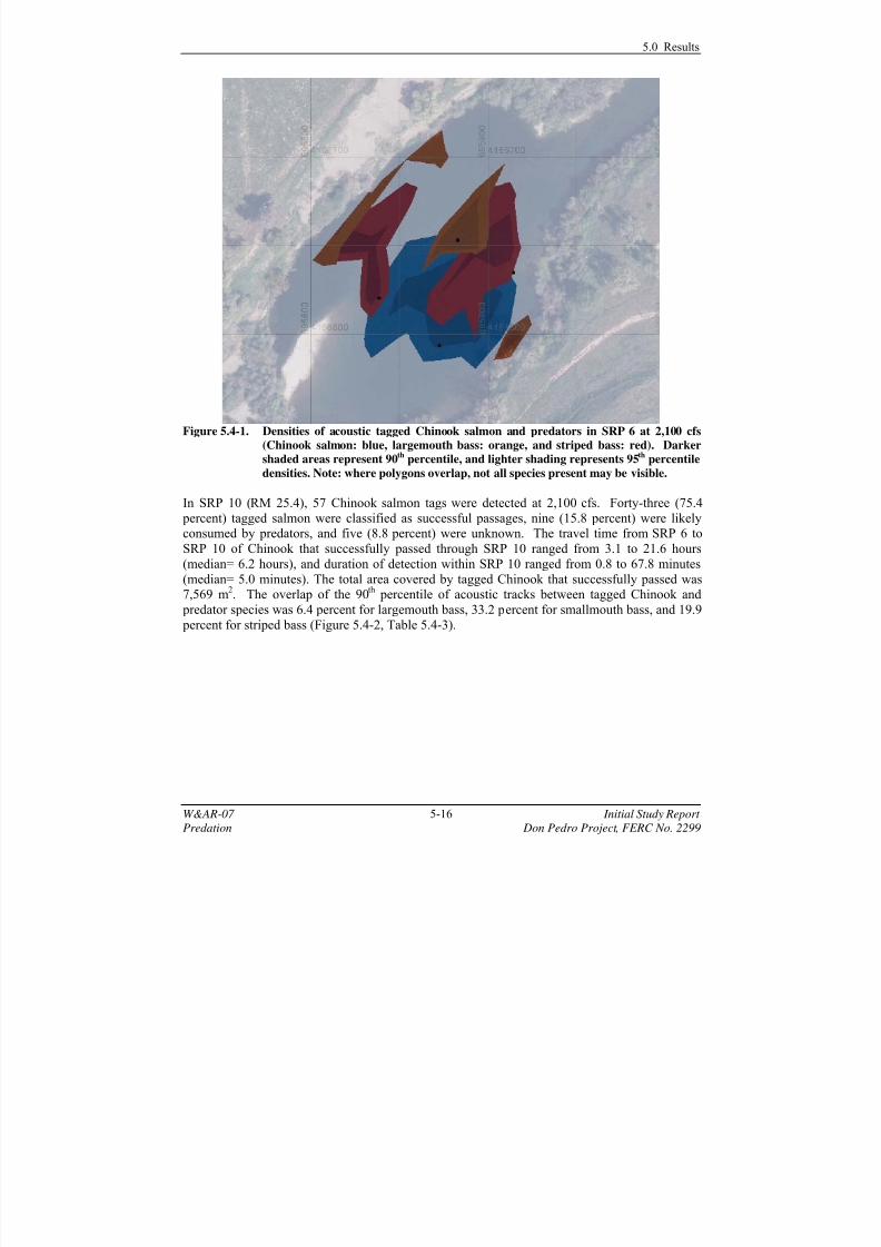
7/29/2019 2013 Predation Study on the Don Pedro Project
http://slidepdf.com/reader/full/2013-predation-study-on-the-don-pedro-project 52/71
5.0 Results
W&AR-07 5-16 Initial Study Report
Predation Don Pedro Project, FERC No. 2299
Figure 5.4-1. Densities of acoustic tagged Chinook salmon and predators in SRP 6 at 2,100 cfs
(Chinook salmon: blue, largemouth bass: orange, and striped bass: red). Darker
shaded areas represent 90th
percentile, and lighter shading represents 95th
percentile
densities. Note: where polygons overlap, not all species present may be visible.
In SRP 10 (RM 25.4), 57 Chinook salmon tags were detected at 2,100 cfs. Forty-three (75.4 percent) tagged salmon were classified as successful passages, nine (15.8 percent) were likelyconsumed by predators, and five (8.8 percent) were unknown. The travel time from SRP 6 to
SRP 10 of Chinook that successfully passed through SRP 10 ranged from 3.1 to 21.6 hours
(median= 6.2 hours), and duration of detection within SRP 10 ranged from 0.8 to 67.8 minutes
(median= 5.0 minutes). The total area covered by tagged Chinook that successfully passed was7,569 m
2. The overlap of the 90
thpercentile of acoustic tracks between tagged Chinook and
predator species was 6.4 percent for largemouth bass, 33.2 percent for smallmouth bass, and 19.9
percent for striped bass (Figure 5.4-2, Table 5.4-3).
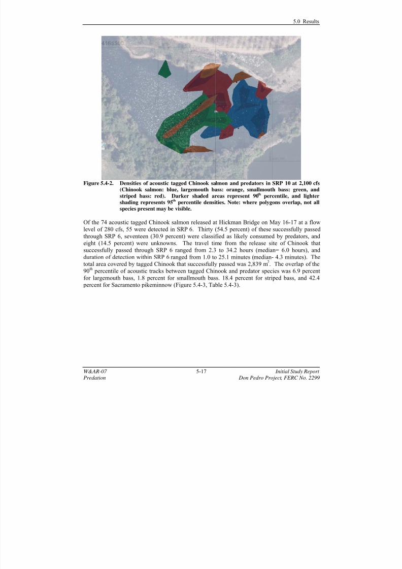
7/29/2019 2013 Predation Study on the Don Pedro Project
http://slidepdf.com/reader/full/2013-predation-study-on-the-don-pedro-project 53/71
5.0 Results
W&AR-07 5-17 Initial Study Report
Predation Don Pedro Project, FERC No. 2299
Figure 5.4-2. Densities of acoustic tagged Chinook salmon and predators in SRP 10 at 2,100 cfs
(Chinook salmon: blue, largemouth bass: orange, smallmouth bass: green, and
striped bass: red). Darker shaded areas represent 90th
percentile, and lighter
shading represents 95th
percentile densities. Note: where polygons overlap, not all
species present may be visible.
Of the 74 acoustic tagged Chinook salmon released at Hickman Bridge on May 16-17 at a flow
level of 280 cfs, 55 were detected in SRP 6. Thirty (54.5 percent) of these successfully passedthrough SRP 6, seventeen (30.9 percent) were classified as likely consumed by predators, andeight (14.5 percent) were unknowns. The travel time from the release site of Chinook that
successfully passed through SRP 6 ranged from 2.3 to 34.2 hours (median= 6.0 hours), and
duration of detection within SRP 6 ranged from 1.0 to 25.1 minutes (median- 4.3 minutes). Thetotal area covered by tagged Chinook that successfully passed was 2,839 m
2. The overlap of the
90th
percentile of acoustic tracks between tagged Chinook and predator species was 6.9 percent
for largemouth bass, 1.8 percent for smallmouth bass. 18.4 percent for striped bass, and 42.4
percent for Sacramento pikeminnow (Figure 5.4-3, Table 5.4-3).
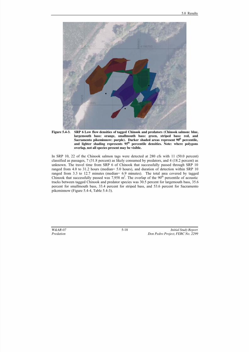
7/29/2019 2013 Predation Study on the Don Pedro Project
http://slidepdf.com/reader/full/2013-predation-study-on-the-don-pedro-project 54/71
5.0 Results
W&AR-07 5-18 Initial Study Report
Predation Don Pedro Project, FERC No. 2299
Figure 5.4-3. SRP 6 Low flow densities of tagged Chinook and predators (Chinook salmon: blue,
largemouth bass: orange, smallmouth bass: green, striped bass: red, and
Sacramento pikeminnow: purple). Darker shaded areas represent 90th
percentile,
and lighter shading represents 95th percentile densities. Note: where polygonsoverlap, not all species present may be visible.
In SRP 10, 22 of the Chinook salmon tags were detected at 280 cfs with 11 (50.0 percent)
classified as passages, 7 (31.8 percent) as likely consumed by predators, and 4 (18.2 percent) as
unknown. The travel time from SRP 6 of Chinook that successfully passed through SRP 10ranged from 4.0 to 31.2 hours (median= 5.0 hours), and duration of detection within SRP 10
ranged from 3.3 to 12.7 minutes (median= 6.9 minutes). The total area covered by tagged
Chinook that successfully passed was 7,958 m2. The overlap of the 90
thpercentile of acoustic
tracks between tagged Chinook and predator species was 30.5 percent for largemouth bass, 35.6
percent for smallmouth bass, 33.4 percent for striped bass, and 53.6 percent for Sacramento
pikeminnow (Figure 5.4-4, Table 5.4-3).

7/29/2019 2013 Predation Study on the Don Pedro Project
http://slidepdf.com/reader/full/2013-predation-study-on-the-don-pedro-project 55/71
5.0 Results
W&AR-07 5-19 Initial Study Report
Predation Don Pedro Project, FERC No. 2299
Figure 5.4-4. SRP 10 Low flow densities of tagged Chinook and predators (Chinook salmon: blue,
largemouth bass: orange, smallmouth bass: green, and striped bass: red). Darker
shaded areas represent 90th
percentile, and lighter shading represents 95th
percentile
densities. Note: where polygons overlap, not all species present may be visible.
Of 73 acoustic tagged Chinook salmon released on May 21–22, 2012 at 415 cfs, 63 Chinook were detected in SRP 6. Twenty (31.7 percent) were classified as successful passages 38 (60.3
percent) were classified as likely consumed by predators and 5 (7.9 percent) were unknowns.
The travel time from the release site of fish that successfully passed through SRP 6 ranged from2.3 to 12.0 hours (median- 6.9 hours) and duration of detection within SRP 6 ranged from 0.4 to
42.7 minutes (median= 6.5 minutes). The total area covered by tagged Chinook that successfully
passed was 4,037 m2. The overlap of the 90
thpercentile of acoustic tracks between tagged
Chinook and predator species was 16.6 percent for largemouth bass, 38.2 percent for smallmouth
bass, and 39.1 percent for striped bass (Figure 5.4-5, Table 5.4-3).
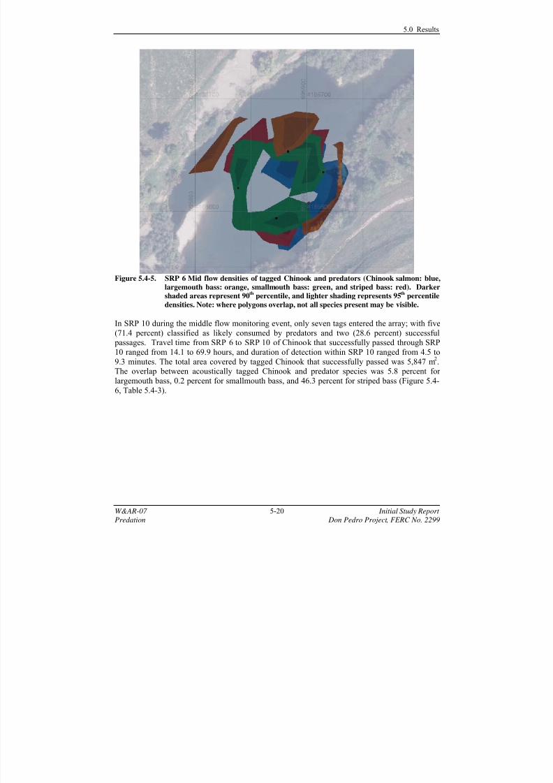
7/29/2019 2013 Predation Study on the Don Pedro Project
http://slidepdf.com/reader/full/2013-predation-study-on-the-don-pedro-project 56/71
5.0 Results
W&AR-07 5-20 Initial Study Report
Predation Don Pedro Project, FERC No. 2299
Figure 5.4-5. SRP 6 Mid flow densities of tagged Chinook and predators (Chinook salmon: blue,
largemouth bass: orange, smallmouth bass: green, and striped bass: red). Darker
shaded areas represent 90th
percentile, and lighter shading represents 95th
percentile
densities. Note: where polygons overlap, not all species present may be visible.
In SRP 10 during the middle flow monitoring event, only seven tags entered the array; with five
(71.4 percent) classified as likely consumed by predators and two (28.6 percent) successful passages. Travel time from SRP 6 to SRP 10 of Chinook that successfully passed through SRP
10 ranged from 14.1 to 69.9 hours, and duration of detection within SRP 10 ranged from 4.5 to
9.3 minutes. The total area covered by tagged Chinook that successfully passed was 5,847 m2.
The overlap between acoustically tagged Chinook and predator species was 5.8 percent for
largemouth bass, 0.2 percent for smallmouth bass, and 46.3 percent for striped bass (Figure 5.4-
6, Table 5.4-3).
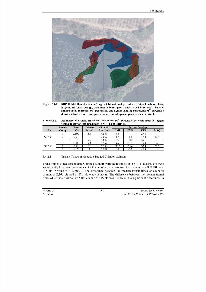
7/29/2019 2013 Predation Study on the Don Pedro Project
http://slidepdf.com/reader/full/2013-predation-study-on-the-don-pedro-project 57/71
5.0 Results
W&AR-07 5-21 Initial Study Report
Predation Don Pedro Project, FERC No. 2299
Figure 5.4-6. SRP 10 Mid flow densities of tagged Chinook and predators (Chinook salmon: blue,
largemouth bass: orange, smallmouth bass: green, and striped bass: red). Darker
shaded areas represent 90th
percentile, and lighter shading represents 95th
percentile
densities. Note: where polygons overlap, not all species present may be visible.
Table 5.4-3. Summary of overlap in habitat use at the 90th
percentile between acoustic tagged
Chinook salmon and predators in SRP 6 and SRP 10.
Site
Release
Group
Flow
(cfs)
Chinook
Passed
Chinook
Area (m2)
Percent Overlap
LMB SMB STB SASQ
SRP 6
1 2,100 63 4,546 8.0 --- 27.4 ---
2 280 31 2,839 6.9 1.8 18.4 42.4
3 415 26 4,037 16.6 38.2 39.1 ---
SRP 10
1 2,100 43 7,569 6.4 33.2 19.9 ---
2 280 11 7,958 30.5 35.6 33.4 53.6
3 415 2 5,847 5.8 0.2 46.3 ---
5.4.2.1
Transit Times of Acoustic Tagged Chinook Salmon
Transit times of acoustic tagged Chinook salmon from the release site to SRP 6 at 2,100 cfs were
significantly less than transit times at 280 cfs (Wilcoxon rank sum test, p-value = < 0.00001) and415 cfs (p-value = < 0.00001). The difference between the median transit times of Chinook
salmon at 2,100 cfs and at 280 cfs was 4.3 hours. The difference between the median transit
times of Chinook salmon at 2,100 cfs and at 415 cfs was 6.2 hours. No significant differences in

7/29/2019 2013 Predation Study on the Don Pedro Project
http://slidepdf.com/reader/full/2013-predation-study-on-the-don-pedro-project 58/71
5.0 Results
W&AR-07 5-22 Initial Study Report
Predation Don Pedro Project, FERC No. 2299
median transit times of Chinook salmon were found between flows of 280 cfs and 415 cfs (p-
value = 0.883) (Figure 5.4-7).
No significant differences in median transit times between SRP 6 and SRP 10 were found
between 2,100 cfs and 280 cfs (Wilcoxon rank sum test, p-value = 0.3588) (Figure 5.4-8). The
sample size of fish arriving at SRP 10 at 415 cfs was too small (n=2) for comparison.
Figure 5.4-7. Transit times from Hickman Bridge to SRP 6 of acoustic tagged juvenile Chinook
salmon (n = 109 total; n = 59 at 2,100 cfs; n = 30 at 280 cfs; and, n = 20 at 415 cfs).
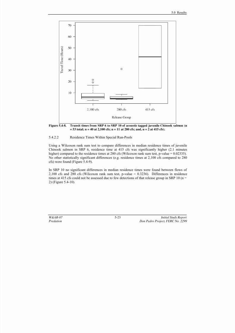
7/29/2019 2013 Predation Study on the Don Pedro Project
http://slidepdf.com/reader/full/2013-predation-study-on-the-don-pedro-project 59/71
5.0 Results
W&AR-07 5-23 Initial Study Report
Predation Don Pedro Project, FERC No. 2299
Figure 5.4-8. Transit times from SRP 6 to SRP 10 of acoustic tagged juvenile Chinook salmon (n
= 53 total; n = 40 at 2,100 cfs; n = 11 at 280 cfs; and, n = 2 at 415 cfs).
5.4.2.2 Residence Times Within Special Run-Pools
Using a Wilcoxon rank sum test to compare differences in median residence times of juvenile
Chinook salmon in SRP 6, residence time at 415 cfs was significantly higher (2.1 minutes
higher) compared to the residence times at 280 cfs (Wilcoxon rank sum test, p-value = 0.02335). No other statistically significant differences (e.g. residence times at 2,100 cfs compared to 280
cfs) were found (Figure 5.4-9).
In SRP 10 no significant differences in median residence times were found between flows of
2,100 cfs and 280 cfs (Wilcoxon rank sum test, p-value = 0.3236). Differences in residencetimes at 415 cfs could not be assessed due to few detections of that release group in SRP 10 (n =
2) (Figure 5.4-10).

7/29/2019 2013 Predation Study on the Don Pedro Project
http://slidepdf.com/reader/full/2013-predation-study-on-the-don-pedro-project 60/71
5.0 Results
W&AR-07 5-24 Initial Study Report
Predation Don Pedro Project, FERC No. 2299
Figure 5.4-9. Residence times (in minutes) at SRP 6 of acoustic tagged juvenile Chinook salmon
(n = 109 total; n = 59 for 2,100 cfs; n = 30 for 280 cfs; and, n = 20 for 415 cfs).
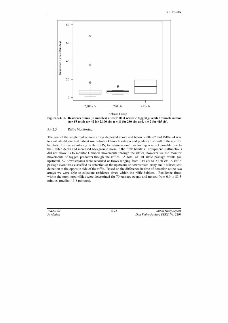
7/29/2019 2013 Predation Study on the Don Pedro Project
http://slidepdf.com/reader/full/2013-predation-study-on-the-don-pedro-project 61/71
5.0 Results
W&AR-07 5-25 Initial Study Report
Predation Don Pedro Project, FERC No. 2299
Figure 5.4-10. Residence times (in minutes) at SRP 10 of acoustic tagged juvenile Chinook salmon
(n = 55 total; n = 42 for 2,100 cfs; n = 11 for 280 cfs; and, n = 2 for 415 cfs).
5.4.2.3
Riffle Monitoring
The goal of the single hydrophone arrays deployed above and below Riffle 62 and Riffle 74 was
to evaluate differential habitat use between Chinook salmon and predator fish within these riffle
habitats. Unlike monitoring in the SRPs, two-dimensional positioning was not possible due tothe limited depth and increased background noise in the riffle habitats. Equipment malfunctions
did not allow us to monitor Chinook movements through the riffles, however we did monitor
movements of tagged predators though the riffles. A total of 101 riffle passage events (44upstream, 57 downstream) were recorded at flows ranging from 244 cfs to 2,160 cfs. A riffle
passage event was classified as detection at the upstream or downstream array and a subsequent
detection at the opposite side of the riffle. Based on the difference in time of detection at the twoarrays we were able to calculate residence times within the riffle habitats. Residence times
within the monitored riffles were determined for 70 passage events and ranged from 0.9 to 83.5
minutes (median 15.8 minutes).

7/29/2019 2013 Predation Study on the Don Pedro Project
http://slidepdf.com/reader/full/2013-predation-study-on-the-don-pedro-project 62/71
W&AR-07 6-1 Initial Study Report
Predation Don Pedro Project, FERC No. 2299
6.0 DISCUSSION AND FINDINGS
6.1 Predator Abundance
6.1.1 Riverwide Abundance Estimates
In 1990, largemouth bass abundance was estimated for the entire lower Tuolumne River (RM 0.0
to RM 52.0) based on shoreline lengths (TID/MID 1992). The abundance estimate for
largemouth bass was 11,074 (Table 2; TID/MID 1992). During 2012, abundance of largemouth
bass from RM 0.0 to RM 39.4 was estimated to be 3,323 based on shoreline length and 3,891 based on habitat area. However differences in study methods preclude making any conclusions
based on comparison of these estimates. Notable differences include no use of block nets to
create a closed population during the 1990 study, differences in geographic scope of sampling,and differences in length criteria used to estimate abundance.
For instance, the 1990 study included largemouth bass between 100 and 150 mm, whereas the
2012 study only estimated abundance of largemouth bass >150 mm. Bass <150 mm were notidentified to species during 2012, and the estimated abundance of bass <150 mm (all species
combined) was 95,198-121, and 756.
Capture rates of smallmouth bass, striped bass, and Sacramento pikeminnow were insufficient to
produce abundance estimates during the 1990 study so no comparison can be made to estimated
abundance in 2012.
6.1.2 Site-specific Abundance Estimates
Site-specific abundance estimates of piscivore-size (> 150 mm FL) largemouth bass ranged from
0 to 42 across 12 sites sampled (Table 5.2-2). McBain & Trush and Stillwater Sciences (2006)used similar depletion methods and reported that site-specific estimates of piscivore-size (180-380 mm FL) largemouth bass ranged from 0 to 18 in 1998 (5 sites sampled); from 2 to 40 in
1999 (6 sites sampled); and, from 5 to 95 in 2003 (6 sites sampled). Using various mark-
recapture estimation methods, TID/MID (1992) reported that site-specific estimates averaged 80
largemouth bass (range = 11 – 181 largemouth bass).
Site-specific abundance estimates of piscivore-size (> 150 mm FL) smallmouth bass ranged from
2 to 50 across 12 sites sampled during late summer 2012 (Table 5.2-3). Site-specific estimates of piscivore-size (180-380 mm FL) smallmouth bass ranged from 0 to 2 in 1998 (5 sites sampled);
from 0 to 13 in 1999 (6 sites sampled); and, from 2 to 49 in 2003 (6 sites sampled) (McBain &
Trush and Stillwater Sciences 2006). Previous research, conducted by TID/MID (1992), showedthat site-specific abundance estimates averaged 20 smallmouth bass (range = 9 – 29 smallmouth
bass).
Site-specific abundance estimates of both Sacramento pikeminnow and striped bass are provided
in Tables 5.2-4 and 5.2-5. We attempted to compare these estimates with previous estimates
from McBain & Trush and Stillwater Sciences (2006), however, differences in length criteria for
Sacramento pikeminnow and very low capture rates of striped bass during 1998, 1999, and 2003
7/29/2019 2013 Predation Study on the Don Pedro Project
http://slidepdf.com/reader/full/2013-predation-study-on-the-don-pedro-project 63/71
6.0 Discussion and Findings
W&AR-07 6-2 Initial Study Report
Predation Don Pedro Project, FERC No. 2299
(McBain & Trush and Stillwater Sciences 2006) do not allow for meaningful comparison.
6.1.3 Smallmouth and Largemouth Bass Densities
Density estimates for largemouth bass and smallmouth bass reported by McBain & Trush and
Stillwater Sciences (2006) were converted from number of fish per 1000 ft of shoreline tonumber of fish per shoreline mile for comparison (Tables 5.2-2 and 5.2-3). However, densities
calculated in the 2012 study used piscivores defined as 150 mm FL and above whereas the
densities calculated in the McBain & Trush and Stillwater Sciences (2006) study used only piscivores between 180 and 380 mm TL.
Density estimates (converted to fish per mile) from McBain & Trush and Stillwater Sciences
(2006) for smallmouth bass (collected in 1998, 1999, and 2003) ranged from 2 to 97 fish per
mile. In comparison, site-specific density estimates of smallmouth bass from the current studyranged from 0 to 251 fish per mile (Table 5.2-3). For largemouth bass, site-specific density
estimates ranged from 0 to 218 largemouth bass per mile, compared with 4 to 196 largemouth
bass per mile (Table 12; McBain & Trush and Stillwater Sciences, 2006) (Table 5.2-2).
6.1.4 General Spatial Distribution
Twelve sites total were sampled for the predator abundance study from RM 3.7 to RM 38.4
during late July and early August 2012. Potential spatial patterns in presence and absence of
target predator species emerged from examining Tables 5.2-2 through 5.2-5. Of the 12 sites,smallmouth bass and striped bass (> 150 mm FL) were captured at 12 and 4 sites, respectively.
The capture locations of striped bass, however, were located in the entire reach, from RM 3.7 to
RM 35.0. Similarly, capture locations of smallmouth bass were located from RM 3.7 to RM
38.4. In contrast, no largemouth bass (> 150 mm FL) were captured at or above RM 34.8 and noSacramento pikeminnow (> 150 mm FL) were captured at or below RM 25.5.
If the spatial distributions of striped bass and smallmouth bass are nearly river wide, this may
have implications for relating their predation rates with their relative abundances. One important
assumption, however, is that the distribution of target species during abundance sampling (latesummer) was relatively similar to the distribution during predation rate sampling (early to mid
Spring). The combination of smallmouth bass and striped bass may account for more predation
on juvenile Chinook salmon due to the combination of their widespread distribution, predationrates, and relative abundance. The distribution of largemouth bass during late summer may be
determined in some part by river location (e.g. more largemouth bass in lower gradient, warmer
lower reaches of the Tuolumne). Likewise, the distribution of Sacramento pikeminnow duringlate summer may be confined to the mid- to upper-portions of the lower Tuolumne River.
6.2 Predation Rate
Predation frequencies (# of predators with at least one Chinook salmon / total # of predators)were significantly higher in SRPs compared to RPs during March 2012, although no evidence of
a difference in predation frequencies by habitat type was detected in May (Figure 5.3-6). No
statistically significant differences in predation frequencies were found between sampling eventsor between habitat types when combined across sampling events.
7/29/2019 2013 Predation Study on the Don Pedro Project
http://slidepdf.com/reader/full/2013-predation-study-on-the-don-pedro-project 64/71
6.0 Discussion and Findings
W&AR-07 6-3 Initial Study Report
Predation Don Pedro Project, FERC No. 2299
Predation rates (# of Chinook salmon per predator) were generally highest for striped bass,
followed by predation rates of smallmouth bass and largemouth bass. Average consumption per predator (not scaled by gastric evacuation rates) in a previous study ranged from 0 to 1.67
(TID/MID 1992; Table 3) compared to 0 to 1.2 in this study with striped bass having the three
highest consumption rates (Table 5.3-3). Juvenile Chinook salmon consumption rates for
largemouth and smallmouth bass (0 – 0.16) observed in this study were lower compared to theconsumption rates for those species (0 – 1.67) in the TID/MID (1992) report. A review by Carey
et al. (2011; Table 4) reported that predation rates (number Chinook salmon consumed per day)
for smallmouth bass from Columbia River basin ranged from 0 to 3.89 Chinook consumed per day, with most values less than 0.1 Chinook salmon per day. The predation rate for striped bass
on juvenile Chinook salmon in the lower Tuolumne River was reported to be zero (TID/MID
1992). However, only eight striped bass were examined in the course of that earlier study. Nostriped bass were captured during predation rate sampling subsequently conducted by Stillwater
Sciences and McBain & Trush (2006).
Chinook salmon were only detected in the stomach samples of smallmouth bass, largemouth
bass, and striped bass. No predation on juvenile Chinook salmon by Sacramento pikeminnowwas observed, however, only six individuals were sampled. Previous research indicates that
predation on juvenile Chinook salmon by Sacramento pikeminnow may be quite low in the lower Tuolumne River. Of 68 Sacramento pikeminnow captured and examined for the presence of
juvenile Chinook salmon in 1992, none were found to have consumed juvenile Chinook salmon
(TID/MID 1992). No Sacramento pikeminnow were captured during predation rate samplingconducted by Stillwater Sciences and McBain & Trush (2006).
Water temperatures were between 13°C and 16°C during the first sampling period (March 22 – March 29) among the sampling locations. During the second sampling period (May 1 – May 9),
water temperatures ranged from 14°C to 17°C among the sampling locations. The water temperatures observed during this study may have partially influenced the predation rate
compared with previous work conducted by Stillwater Sciences and McBain & Trush (2006). In
that study, very few target species (n = 4) were captured, but of those captured, none contained juvenile salmon. Water temperatures were much lower during the earlier study, ranging from
10.7°C to 12.8°C, compared to 13°C to 17°C observed in the current study (Figure 5.1-2).
Discharge during the previous study was significantly higher (6,740 cfs to 9,120 cfs) than
discharges observed during predation rate sampling in this study (about 350 cfs to about 2,100cfs) (Figure 5.1-1).
Turbidity during predation rate sampling ranged from 0.77 NTU to 2.83 NTU, and these levelswere similar to those reported in the TID/MID (1992) study. The results of neither study
suggested any connection between predation rates and turbidity, and while the ranges of turbidity
during sampling were quite narrow, they are representative of the range of typical baselineturbidity conditions in the lower Tuolumne River. Other studies have found that turbidity greater
than 25 NTU reduces the incidence and risk of piscivory on salmonid prey (Gregory and Levings
1998).

7/29/2019 2013 Predation Study on the Don Pedro Project
http://slidepdf.com/reader/full/2013-predation-study-on-the-don-pedro-project 65/71
6.0 Discussion and Findings
W&AR-07 6-4 Initial Study Report
Predation Don Pedro Project, FERC No. 2299
6.2.1 Diet Composition
Invertebrates (insects and crayfish) made up a large portion (by frequency of occurrence and by
total count) of identifiable prey items among the stomach samples examined. Crayfish were
present in about 26 percent of all stomach samples from the target species examined. This result
is similar to the TID/MID (1992) report, where 17 percent and 33 percent of fish sampled(consisting of smallmouth bass, largemouth bass, Sacramento pikeminnow, striped bass, bluegill,
redear sunfish, green sunfish, channel catfish, white catfish, and brown bullhead) contained
crayfish.
Thirty fish identified as juvenile Chinook salmon occurred in about 12 percent of the stomach
samples or 30 of the 246 non-empty stomach samples examined. However, juvenile Chinook salmon only made up about 10 percent of all the fish (n = 326) observed in stomach samples.
Other fish consumed were unidentified larval fish (observed in 79 of 246 non-empty stomachs),
sculpin (16 of 246), and lamprey and cyprinids (2 of 246).
6.3
Synthesizing Abundance and Predation Rates
The cumulative impact of predation was assessed by estimating the abundance of target species
between RM 5.1 (location of the Grayson rotary screw trap) and RM 30.3 (location of theWaterford rotary screw trap). Methods to estimate abundance based on shoreline lengths in this
reach are described in Section 4.2.2.3. The abundance in this reach was then combined with the
species-specific predation rates observed in this study (see Sections 4.3.3.3 and 5.3.6 “Predationrates on juvenile Chinook salmon”).
We estimated abundance of predatory fish based on a total shoreline distance (feet) of 298,163 between the Waterford and Grayson rotary screw traps. Density estimates of predators were
calculated using only site-specific abundance estimates from sites sampled between RM 5.1 andRM 30.3, so that abundance data from only seven of the twelve sites was used. All estimators for
abundance and variance for this calculation are provided in Section 4.2.2.3.
Abundance estimates of piscivore-sized fish (>150 mm FL) between Waterford and Grayson
were 3,013 largemouth bass (SE156), 117 (SE18) Sacramento pikeminnow, 3,626 (SE111)smallmouth bass, and 235 (SE21) striped bass. Species-specific predation rates for the lower
predation rate (e.g. the rate based on a 20-hour gastric evacuation time) were averaged for allhabitat types and sampling events. Predation rates were 0.10 Chinook per predator per day for
largemouth bass, 0.0 Chinook per predator per day for Sacramento pikeminnow, 0.11 Chinook
per predator per day for smallmouth bass, and 1.1 Chinook per predator per day for striped bass(see Table 5.3-3). To be conservative in the cumulative impact assessment of predation between
the two rotary screw traps, we used the lower 95 percent confidence bounds for each species
abundance estimate which were 21,701 largemouth bass, 81 Sacramento pikeminnow, 3,404smallmouth bass and 193 striped bass. The total estimate of juvenile Chinook salmon potentially
consumed was estimated by multiplying the number of predators, the migration period (in days),
and the estimated predation rate (in number of juvenile Chinook salmon consumed per day). For
example, the estimated number of juvenile Chinook salmon consumed by largemouth bass over a90-day migratory period was 24,309 (2,701 * 90 * 0.1). We used 60-, 90-, or 120-day migratory

7/29/2019 2013 Predation Study on the Don Pedro Project
http://slidepdf.com/reader/full/2013-predation-study-on-the-don-pedro-project 66/71
6.0 Discussion and Findings
W&AR-07 6-5 Initial Study Report
Predation Don Pedro Project, FERC No. 2299
periods which assumed that the daily numbers of juvenile Chinook migrating was uniformly
distributed and that all equally vulnerable to predation at the average rate.
The estimated numbers of juvenile Chinook consumed in the reach between the Waterford and
Grayson rotary screw traps are reported in Table 6.3-1. Despite making up only a small fraction
(< 4 percent) of the total of piscivore-sized fish (> 150 mm FL), striped bass were estimated toconsume nearly 25 percent of the total potential juvenile Chinook salmon consumed.
Smallmouth bass were estimated to consume about 44 percent of juvenile Chinook salmon and
largemouth bass were estimated to consume about 32 percent of juvenile Chinook salmon.
Table 6.3-1. Estimated cumulative impact of predation in the lower Tuolumne River between
RM 30.3 and RM 5.1 under a low predation rate (gastric evacuation time set at 20-
hours) by length of migratory period of juvenile Chinook salmon.
Species ˆ N
Predation
Rate
60-Day
Migratory
Period
90-Day
Migratory
Period
120-Day
Migratory
Period
Percent
of
Impact
Largemouth bass 2,701 0.1 16,206 24,309 32,412 31.5%
Sacramento pikeminnow 81 0 0 0 0 0.0%Smallmouth bass 3,404 0.11 22,466 33,700 44,933 43.7%
Striped bass 193 1.1 12,738 19,107 25,476 24.8%
Total 51,410 77,116 102,821
Total potential consumption of juvenile Chinook salmon was estimated to be about 77,000 for a
90-day migratory period (Table 6.3-1). Estimated abundance of juvenile Chinook salmon at the
Waterford rotary screw trap during January 3 - June 15, 2012 was 68,650, suggesting thatconsumption of juvenile Chinook salmon by predators between the Waterford and Grayson
rotary screw traps could equal or exceed the number passing the Waterford trap. Only 2,969
Chinook salmon were estimated to have survived migration through the 25 miles between the
trapping sites (Sonke and Fuller 2012), making it plausible that most, if not all, losses of juvenileChinook salmon in the lower Tuolumne River between Waterford and Grayson during 2012
could be attributed to non-native predatory species.
Predation rate sampling and predator abundance sampling did not temporally overlap, it was
assumed that predator abundance in summer was similar to predator abundance during the
juvenile Chinook salmon migration. Given the similarity in densities of predatory species between this study and previous studies conducted on the lower Tuolumne River, and the
similarities between predation rates between this study and other predation rates observed from
the same species, we feel justified that the cumulative impacts of predation on juvenile Chinook
salmon in the lower Tuolumne River during the spring of 2012 were substantial.
Losses of juvenile Chinook salmon between the rotary screw traps at Waterford and Grayson
ranged between approximately 76 percent and 98 percent during 2007-2011, with the actualnumbers of individuals estimated to be lost ranging from approximately 22,000 to 330,000. If the
predation rates and predator abundances in these years were similar to those documented in the
2012 study, it is plausible that the overwhelming majority of Chinook salmon mortality was dueto predation.
7/29/2019 2013 Predation Study on the Don Pedro Project
http://slidepdf.com/reader/full/2013-predation-study-on-the-don-pedro-project 67/71
6.0 Discussion and Findings
W&AR-07 6-6 Initial Study Report
Predation Don Pedro Project, FERC No. 2299
6.4 Differential Habitat Use
Two-dimensional acoustic tracking was used to evaluate the role of flow in segregating potential predators from outmigrating Chinook salmon within the special run-pools. Results showed
overlap between acoustically tagged Chinook and predators at the three tested flows (280 cfs,
415 cfs, and 2,100 cfs). Striped bass were found to have the greatest overlap in habitat use withChinook salmon (18.4 percent - 46.3 percent), followed by largemouth bass (5.8 percent -30.5 percent), and smallmouth (0.2 percent - 38.2 percent).
Residence times of Chinook salmon within SRPs were also found to be similar between releasegroups, with the only significant difference in the medians found between 415 cfs and 280 cfs in
SRP 6. It should be noted that the highest range in residence times at both SRPs was found
during the 2,100 cfs event. Based on review of individual acoustic tracks, extended residencetimes were due to fish circling within the array rather than passing directly through the SRP.
Circling was likely caused by hydraulic conditions within the SRPs at the higher flows.
An earlier study on the Tuolumne River (McBain & Trush and Stillwater Sciences, 2006)hypothesized that at flows exceeding 300 cfs, higher velocities would increase Chinook salmon
migration rates through SRP sites. The results of this study do not support this hypothesis as
transit times across SRP 6 and SRP 10 were fastest at 280 cfs, suggesting that higher flowsactually decrease transit rates through the SRPs. Comparison of transit rates at each site at a
given flow found no statistically significant difference in transit rates between sites, suggesting
that this trend may also apply to other SRP sites that were not studied in 2012.
Acoustic detections within riffle 62 and riffle 74 and estimated residence times within riffles
suggest that predator species (largemouth bass, smallmouth bass, and striped bass) were able tomove unrestricted through riffle habitats at all test flows. Tracking technology did not allow for
precise determination of tagged fish locations within the riffles.
6.5 Potential Additional Studies to Be Conducted in 2013
The Districts are considering conducting an additional year of predator abundance and predation
rate sampling in 2013 using the same methodology as employed in the 2012 study. It is apparent
from the 2012 results that predation is a significant factor affecting salmon smolt survival on theTuolumne River. Additional information may provide greater detail related to potential
protection, mitigation and enhancement measures.
7/29/2019 2013 Predation Study on the Don Pedro Project
http://slidepdf.com/reader/full/2013-predation-study-on-the-don-pedro-project 68/71
W&AR-07 7-1 Initial Study Report
Predation Study Don Pedro Project, FERC No. 2299
7.0 STUDY VARIANCES AND MODIFICATIONS
The study was conducted consistent with the approved study plan. No variances occurred.
The study is complete. No modifications are proposed.
7/29/2019 2013 Predation Study on the Don Pedro Project
http://slidepdf.com/reader/full/2013-predation-study-on-the-don-pedro-project 69/71
W&AR-07 8-1 Initial Study Report
Predation Don Pedro Project, FERC No. 2299
8.0 REFERENCES
Adams, N. J, D. R. Barton, R. A. Cunjak, G. Power, and S. C. Riley. 1987. Diel patterns of
activity and substrate preference in young Arctic char from the Koroc River, northern
Quebec. Canadian Journal of Zoology 66:2500–2502.
Adams, N.S., D.W. Rondorf, S.D. Evans, and J.E. Kelly. 1998. Effects of Surgically and
Gastrically Implanted radio Transmitters on Growth and Feeding Behavior of JuvenileChinook Salmon. Transactions of the American Fisheries Society 127: 128-136.
Angradi, T. R., and J. S. Griffith. 1990. Diel feeding chronology and diet selection of rainbow
trout (Oncorhynchus mykiss) in the Henry’s Fork of the Snake River, Idaho. CanadianJournal of Fisheries and Aquatic Sciences 47:199–209.
Aragon, T. 2010. epitools: Epidemiology Tools. R package version 0.5-6. http://CRAN.R- project.org/package=epitools
Benkwitt, C.E., R.D. Brodeur, T.P. Hurst, E.A. Daly. 2009. Diel Feeding Chronology, GastricEvacuation, and Daily Food Consumption of Juvenile Chinook Salmon in Oregon Coastal
Waters.
Brown, L.R., and T. Ford. 2002. Effects of flow on the fish communities of a regulated
California river: implications for managing native fishes. River Research and
Applications 18:331-342.
Carey, M. P., B. L. Sanderson, T. A. Friesen, K. A. Barnas, and J. D. Olden. 2011. Smallmouth
bass in the Pacific Northwest: a threat to native species; a benefit for anglers. Reviews in
Fisheries Science 19: 305-315.
Carle, F. L., and M. R. Strub. 1978. A new method for estimating population size from removal
data. Biometrics 34:621-630.
Clark, C. W., and D. A. Levy. 1988. Diel vertical migrations by pelagic planktivorous fishes and
the antipredator window. American Naturalist 131:271–290.
Crawley, M.J. 2007. The R Book. John Wiley & Sons, Inc., New York, New York.
Ehrenberg, J.E. and T.W. Steig. 2003. Improved techniques for studying the temporal and
spatial behavior of fish in a fixed location. ICES J of Mar. Sci, 60: 700-706.
Frost, C.N. 2000. A key for identifying preyfish in the Columbia River based on diagnostic bones. U.S. Geological Survey, Columbia River Research Laboratory, Western Fisheries
Research Center, Cook, Washington, 50 pp.
Gregory, R. S., and C. D. Levings. 1998. Turbidity Reduces Predation on Migrating Juvenile
Pacific Salmon. Transactions of the American Fisheries Society 127:275–285.

7/29/2019 2013 Predation Study on the Don Pedro Project
http://slidepdf.com/reader/full/2013-predation-study-on-the-don-pedro-project 70/71
8.0 References
W&AR-07 8-2 Initial Study Report
Predation Don Pedro Project, FERC No. 2299
Hankin, D.G. 2009. Sampling Theory. Unpublished Manuscript. Preprint from D.G. Hankin,
Department of Fisheries Biology, Humboldt State University, Arcata, CA.
Hansel, H.C., S.D. Duke, P.T. Lofy, and G.A. Gray.1998. Use of diagnostic bones to identify
and estimate original lengths of ingested prey fishes. Transactions of the American
Fisheries Society 117:1, 55-62.
Kamler, J. F. and K. L. Pope. 2001. Nonlethal Methods of Examining Fish Stomach Contents.
Reviews in Fisheries Science 9(1): 1-11.
Martinelli, T.L., H.C. Hansel, and R.S. Shively. 1998. Growth and physiological responses to
surgical and gastric radio transmitter implantation techniques in subyearling Chinook salmon. Hydrobiologia 371/372: 78-87.
McBain & Trush and Stillwater Sciences. 2006. Special Run Pool 9 and 7/11 Reach: post- project monitoring synthesis report. Prepared for the Tuolumne River Technical Advisory
Committee, Turlock and Modesto Irrigation Districts, USFWS Anadromous FishRestoration Program, and California Bay-Delta Authority, by McBain & Trush, Arcata
and Stillwater Sciences, Berkeley, CA.
Ogle, D. H. 2011. fishR Vignette – Depletion Methods for Estimating Abundance. Available
online at: http://www.ncfaculty.net/dogle/fishR/gnrlex/Depletion/Depletion.pdf
R Development Core Team (2010). R: A language and environment for statistical computing. R
Foundation for Statistical Computing, Vienna, Austria.
Särndal, C.E., Swensson, B., and Wretman, J. 1992. Model Assisted Survey Sampling. NewYork: Springer-Verlag.
Sonke, C. and A. Fuller. 2012. Outmigrant Trapping of Juvenile Salmon in the Lower TuolumneRiver, 2012. Prepared for Turlock and Modesto Irrigation Districts by FISHBIO,
Oakdale, CA.
Stillwater Sciences and McBain & Trush. 2006. Lower Tuolumne River Predation AssessmentFinal Report. Prepared for the Tuolumne River Technical Advisory Committee, Turlock
and Modesto Irrigation Districts, USFWS Anadromous Fish Restoration Program, and
California Bay-Delta Authority, by Stillwater Sciences, Berkeley, CA and McBain &Trush, Arcata, CA.
Stillwater Sciences. 2010. Tuolumne River Floodplain Inundation Maps.
Thompson, S.K. 2002. Sampling, 2nd
Edition. John Wiley & Sons, Inc., New York, New York
Turlock Irrigation District and Modesto Irrigation District (TID/MID). 1992. Lower Tuolumne
River Predation Study Report. Appendix 22 to Turlock Irrigation District and Modesto
Irrigation District Pursuant to Article 39 of the License for the Don Pedro Project, No.

7/29/2019 2013 Predation Study on the Don Pedro Project
http://slidepdf.com/reader/full/2013-predation-study-on-the-don-pedro-project 71/71
8.0 References
2299 Vol. VII. Prepared by T. Ford, Turlock and Modesto Irrigation Districts and EA
Engineering, Science, and Technology, Lafayette, California.
U.S. Department of Commerce, National Marine Fisheries Service (NMFS). 2000. Guidelines
for Electrofishing Waters Containing Salmonids Listed Under the Endangered Species
Act. National Marine Fisheries Service. Available online at:http://www.nwr.noaa.gov/ESA-Salmon-Regulations-Permits/4d-
Rules/upload/electro2000.pdf .
Van Den Avyle, M. J. and J. E. Roussel. 1980. Evaluation of a Simple method for removing
food Items from live black bass. Progressive Fish-Cult. 42: 222-223.