17‐760

“ElectoralCompetitionandPartyPositioning”

PhilippeDeDonderandMariaGallego

January2017

Electoral Competition and Party Positioning

Philippe De Donder1 and Maria Gallego2

January 30, 2017

1Toulouse School of Economics, philippe.dedonder@tse-fr.eu.2Department of Economics, Wilfrid Laurier University, mgallego@wlu.ca

Abstract

We survey the literature on the positioning of political parties in uni- and multi-

dimensional policy spaces. We keep throughout the survey the assumption that

there is an exogenous number of parties who commit to implement their policy

proposals once elected. The survey stresses the importance of three modeling

assumptions: (i) the source of uncertainty in election results, (ii) the parties’

objectives (electoral —maximizing their expected vote share, or their probability

of winning the elections—policy oriented or both), and (iii) the voters’preferences

(if and how they care for parties beyond the policies implemented by the winner).

1 Introduction

Most papers in the political economy literature have concentrated on some form of

“median voter theorem”within the so-called Downsian approach, with 2 parties

(or candidates) simultaneously proposing platforms (belonging to unidimensional

policy spaces) to voters and committing to implement their platform if elected.

Moreover, parties are assumed to care only about winning the elections, while

voters care only about policies. Finally, there is no uncertainty in the model,

in the sense that parties can perfectly anticipate the election results at the time

where parties propose their platform.

As mentioned by Roemer (2006), there are many problems associated with this

approach and with the results it generates. Parties do not care for policies, which

contradicts how they have developed historically. There is no room for voters to

care about the identity of the elected party (as opposed to the policy this party

enacts). The lack of electoral uncertainty at the time parties choose their platform

constitutes a very strong assumption. Finally, concerning the results of the model,

the convergence of parties to the same policies is not observed in practice (as we

will show later on in the survey), and this model has generically no equilibrium

in pure strategies as soon as the policy space is multi-dimensional.

The objective of this paper is to survey the literature on the positioning of po-

litical parties in uni- and multi-dimensional policy spaces. We will keep through-

out the survey the assumption that there is an exogenous number of parties who

commit to implement their policy proposals once elected. This survey will stress

the importance of three modeling assumptions: (i) the source of uncertainty in

election results, (ii) the parties’objectives (electoral —maximizing their expected

vote share, or their probability of winning the elections—or policy oriented), and

(iii) the voters’preferences (if and how they care for parties beyond the policies

implemented by the winner). We now turn to the plan of this survey.

1

We describe the general setting and notation used throughout the survey in

section 2. Then show in section 3 that, in the absence of uncertainty, parties con-

verge to the same policy whether they are electorally or policy motivated when

the policy space is unidimensional, and that there is generically no equilibrium in

pure strategies for multidimensional policy spaces. The first conclusion we draw is

that introducing some form of uncertainty as to the election results is primordial.

There are several different ways to introduce uncertainty. The easiest one is to add

some noise to the voters’behavior, irrespective of the policy proposals of the par-

ties. We develop this so-called stochastic partisanship approach in section 4. We

then assume alternatively that parties are uncertain as to the policy preferences

of voters in section 5 where we detail several ways to introduce this uncertainty,

varying in the degree of micro-foundation of the uncertainty, in section 5.1. Such

uncertainty creates a discontinuity in the expected vote/probability of winning

function when both parties propose the same policy, so that there are equilibrium

existence problems when parties are electorally motivated. We then concentrate

on policy motivated parties in section 5.2, and on the case where parties have

both electoral and policy motivations in section 5.3. In both cases, we first deal

with analytical results before mentioning various applications of these models.

We then examine in section 6 models in which candidates’electoral prospects

depend on a valence component—voters’non-policy evaluation of candidates—and

where all voters agree that one party has better characteristics than another.

Section 6.1 is devoted to the study of unidimensional policy spaces. We analyze

in section 6.1.1 the case where there is uncertainty as to the election results, while

section 6.1.2 is devoted to the case where uncertainty concerns the valence of the

candidates. Section 6.2 deals with valence in multidimensional policy spaces. We

present different theoretical models in sections 6.2.1 to 6.2.4, while section 6.2.5

concentrates on a specific empirical application.

2

Finally, in Section 7 we present the “unified model” developed by Adams,

Merrill and Grofman where voters care both for multi-dimensional policies and for

the parties enacting them. More precisely, voters differ in their partisanship, with

some being closer to one party and others to another party, with this partisanship

affecting their policy preferences. Adams et al. also add a random component to

the voters’utility, as in section 4. We start in section 7.1 with the description of

their model, including some analytical results that they obtain. We then move

in section 7.2 to two empirical applications of this model (to the 1988 French

presidential elections, and the 1989 election in Norway). We consider an empirical

extension where valence is added to this unified model (as in sections 6.1.1 and

6.1.2) in section 7.3, before offering a general conclusion in section 8.

2 General setting and notation

We give here the basic setting and notation used throughout the survey. The policy

space is denoted by X and is a subset of the Euclidean space with d dimensions.

X is assumed to be non-empty, convex and compact. There are n voters, where

n can be finite (in which case it is assumed to be odd) or infinite. There are J

political parties, or candidates, with J ≥ 2.1 Since most papers deal with only 2

parties, we use below the notation j ∈ A,B (or A andD in section 6, for reasons

which will become obvious there) whenever possible rather than j ∈ 1, ..., J.

All voters are endowed with a utility function ui(x, j), where x ∈ X and j ∈

A,B. In words, voters care for policies but may also care for the party proposing

the policy. Voter i’s utility function is assumed to be concave over X, and we

denote by xi voter i’s most-preferred policy (also called an ideal or blisspoint).

Note that this blisspoint is independent of the party’s identity. In some sections,

1We will use the terms candidate and party interchangeably throughout the survey.

3

we also assume that preferences are Euclidean, so that voter i’s utility is decreasing

in the distance between the proposed policy x and her blisspoint xi.

All parties simultaneously choose a policy x in X, which we denote by xj,

j ∈ A,B, which they commit to enact if they are elected. Voters observe xjand simultaneously vote for the party that offers them the highest utility level.2

We are looking for Nash equilibria in pure strategies of the game played among

parties. In the absence of such a Nash equilibrium, we will look for either a local

Nash equilibrium (section 6.2.2) or for a Nash equilibrium in mixed strategies.

The parties’objectives may be electoral, policy-related, or both. We consider

two types of electoral motivations: maximizing the probability of winning the

elections (henceforth called the “win motivation”), and the expected number (or

fraction) of votes (the “vote motivation”). We denote by πj(xA, xB) the proba-

bility that party j ∈ A,B wins the election when it proposes policy xA while

its opponent proposes xB, and by EVj(xA, xB) its expected vote. In the case of

policy motivation, we assume that each party j is endowed with a utility function

Uj(x). This utility function will be in most cases given exogenously, but may also

be endogeneized as part of the equilibrium. We denote party j’s most-preferred

policy (i.e., the policy maximizing Uj(x)) as xj, j ∈ A,B).

A very important distinction is between deterministic voting (where all candi-

dates can predict with certainty the voting behavior of all individual voters at the

time where policy platforms are offered) and probabilistic voting (where voting

behavior is modelled as a random variable from the perspective of the candidates,

with parties computing the probability that each voter gets more utility under its

proposal than under its adversary’s). In the latter case, we will talk of aggregate

uncertainty when parties are unable to forecast with certainty the election results

2This behavior, often called sincere voting, corresponds to the elimination of weakly undom-inated strategies when J = 2 and voting is assumed, as here, to be costless. In case severalparties give the same utility to a voter, she fairly randomizes her vote among those parties.

4

at the time where platforms are made public. Observe that probabilistic voting

does not imply aggregate uncertainty: as we will see in section 4, if there is a large

number of voters who are affected by i.i.d. shocks to their utility function, the

voting behavior of any individual voter is stochastic, but their aggregate behavior

(and thus the election results) is known with certainty, thanks to the law of large

numbers. Depending on the model presented, we will either introduce uncertainty

at the micro level (i.e., at the level of the individual voter), or at the macro level

(i.e., at the level of the electorate, without providing the micro-foundations for

this aggregate uncertainty)—see section 5.1.

3 Deterministic voting

In this section, we assume away uncertainty, so that parties know the individual

voters’ preferences and can compute with certainty the voting behavior of all

individuals when choosing their platforms. Moreover, we assume that voters care

only about policies, so that ui(x, j) = ui(x) for all voters i and parties j = A,B.

It is well know since Hotelling (1929) and Downs (1957) that,

Proposition 1 Assume that there is no uncertainty, that d = 1 and that both

parties are electorally motivated (maximizing either their probability of winning

or their number of votes), then there exists a unique Nash equilibrium in pure

strategies where both parties propose the median voter’s ideal point: med(xi).

This result is known as the “median voter theorem.”Moreover, it is also known

since Plott (1967) and Hinich et al (1973), among others,3 that

3McKelvey (1976, 1979), Schofield (1978, 1983, 1985), Cohen and Matthews (1980), McK-elvey and Schofield (1986, 1987), Caplin and Nalebuff (1991), Banks (1995), Saari (1997), andAusten-Smith and Banks (1999). Eaton and Lipsey (1975) also obtained instability results whenthere are three or more candidates.

5

Proposition 2 Assume that there is no uncertainty, that d > 1 and that both

parties are electorally motivated (maximizing either their probability of winning or

their number of votes), then there generically does not exist any Nash equilibrium

in pure strategies.

The generalization of Proposition 1 to a multidimensional setting requires the

existence of a “median in all dimensions” of the policy space. This in turn re-

quires that the distribution of voters’most-preferred policies be radially symmet-

ric, which is an extremely restrictive assumption. Moreover, any move from a ra-

dially symmetric distribution of blisspoints, however small, results in the (generic)

non-existence of an equilibrium in pure strategies.4

As for equilibria in mixed strategies, there is no general existence theorem

because the parties’payoffs are not continuous in general when d > 1. Duggan and

Jackson (2005) show that, if indifferent voters are allowed to randomize with any

probability between zero and one (rather than with 1/2 as often assumed), then

mixed equilibria do exist. Moreover, they show that, starting with a distribution

of individuals such as a Nash equilibrium in pure strategy exists and perturbing

this distribution, then the equilibrium mixed strategies of the parties will put

probabilities arbitrarily close to one on policies near the original equilibrium in

pure strategies. In other words, mixed strategy equilibrium outcomes change in a

continuous way when voter preferences are perturbed.5

What about moving away from electoral preferences towards policy motiva-

tions? Unfortunately, this does not change the results with d = 1, as shown in

the next proposition due to Wittman (1977), Calvert (1985) and Roemer (1994):

4Alternatively, existence may occur when the decision rule requires a suffi ciently large ma-jority (Schofield, 1984; Strand, 1985; Caplin and Nalebuff, 1988).

5McKelvey (1986), Cox (1987), and Banks, Duggan and Le Breton (2002) show that thesupport of the mixed strategy Nash equilibria lies in the uncovered set, a centrally locatedsubset of the policy space.

6

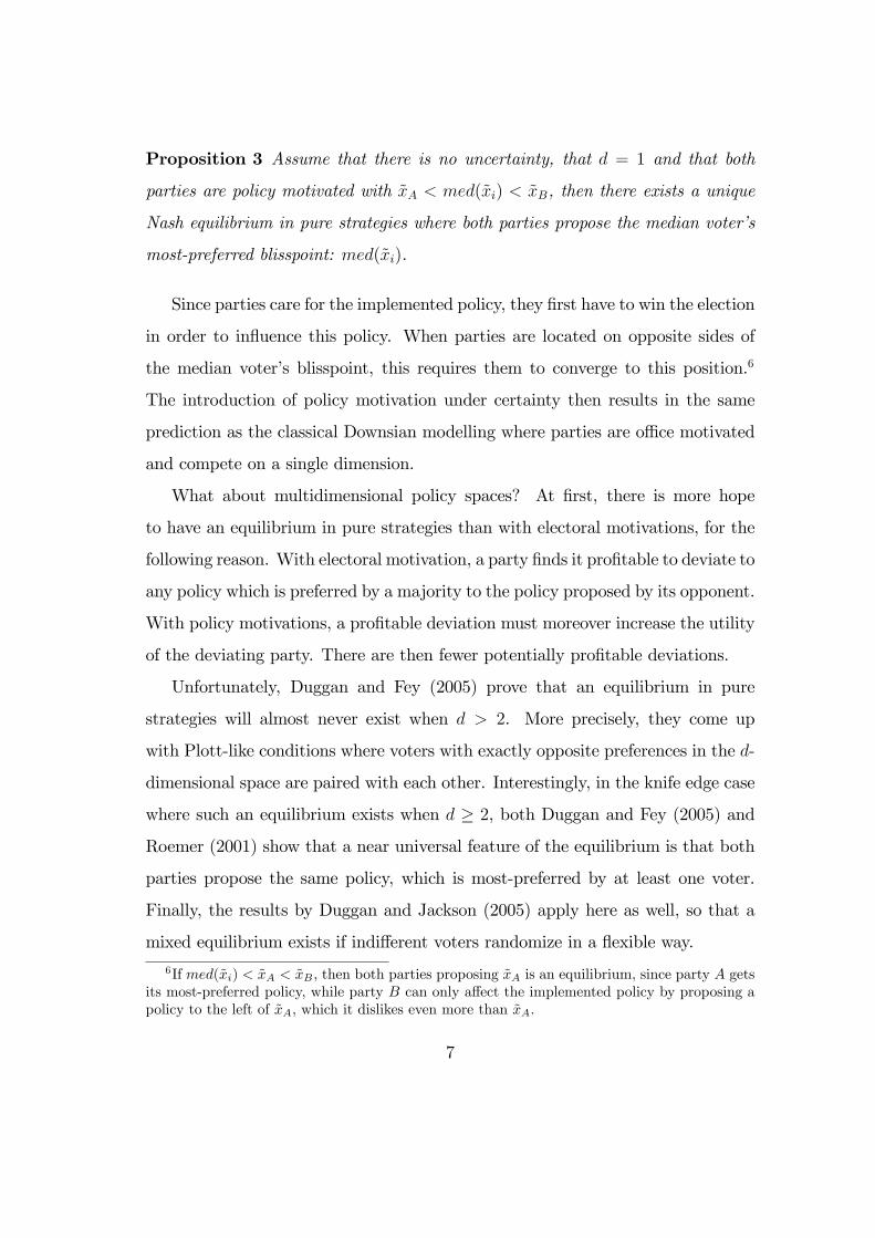
Proposition 3 Assume that there is no uncertainty, that d = 1 and that both

parties are policy motivated with xA < med(xi) < xB, then there exists a unique

Nash equilibrium in pure strategies where both parties propose the median voter’s

most-preferred blisspoint: med(xi).

Since parties care for the implemented policy, they first have to win the election

in order to influence this policy. When parties are located on opposite sides of

the median voter’s blisspoint, this requires them to converge to this position.6

The introduction of policy motivation under certainty then results in the same

prediction as the classical Downsian modelling where parties are offi ce motivated

and compete on a single dimension.

What about multidimensional policy spaces? At first, there is more hope

to have an equilibrium in pure strategies than with electoral motivations, for the

following reason. With electoral motivation, a party finds it profitable to deviate to

any policy which is preferred by a majority to the policy proposed by its opponent.

With policy motivations, a profitable deviation must moreover increase the utility

of the deviating party. There are then fewer potentially profitable deviations.

Unfortunately, Duggan and Fey (2005) prove that an equilibrium in pure

strategies will almost never exist when d > 2. More precisely, they come up

with Plott-like conditions where voters with exactly opposite preferences in the d-

dimensional space are paired with each other. Interestingly, in the knife edge case

where such an equilibrium exists when d ≥ 2, both Duggan and Fey (2005) and

Roemer (2001) show that a near universal feature of the equilibrium is that both

parties propose the same policy, which is most-preferred by at least one voter.

Finally, the results by Duggan and Jackson (2005) apply here as well, so that a

mixed equilibrium exists if indifferent voters randomize in a flexible way.

6If med(xi) < xA < xB , then both parties proposing xA is an equilibrium, since party A getsits most-preferred policy, while party B can only affect the implemented policy by proposing apolicy to the left of xA, which it dislikes even more than xA.

7

The message of this section is thus pretty bleak: if d = 1, we obtain convergence

to the median blisspoint irrespective of the (electoral or policy) motivation of

parties, while there is generically no equilibrium in pure strategies with d > 2.

We now introduce uncertainty, so that parties see the individual voters’be-

havior as random. We first look at situations with stochastic partisanship, then

to stochastic preferences.

4 The stochastic partisanship approach

One way to introduce uncertainty is to assume that uncertainty affects voters’

preferences. This is modeled by assuming that voters’preferences are affected by

a random shock determining the bias the voter has for one of the two parties, the

so-called stochastic partisanship approach.

4.1 Theory

In this section, we assume that voters’preferences are additively separable into

their preferences for policies and for parties, so that with slightly abusing notation,

ui(x, j) =

ui(x) if j = A

ui(x) + γi if j = B

where the vector of party biases (γ1, ..., γn) is seen as a random variable by both

candidates A and B.7 More precisely, both parties have the same beliefs and

assume that each γi is distributed according to the cdf Fi with pdf fi > 0 over

its support. Observe that we do not assume that these biases are independently

distributed. The probability that voter i will vote for party A is then given by

7Coughlin and Nitzan (1982) study the multiplicative formulation, where voter i’s utilityfunction is log-concave with i voting for party A if ui(xA) ≥ ui(xB)γi.Duggan (2014) indeedshows that the two approaches are equivalent, up to a simple transformation.

8

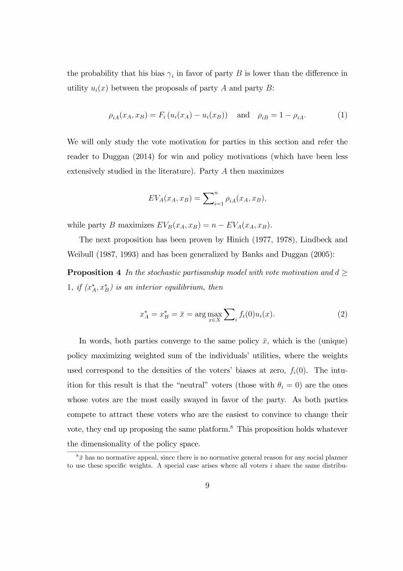
the probability that his bias γi in favor of party B is lower than the difference in

utility ui(x) between the proposals of party A and party B:

ρiA(xA, xB) = Fi (ui(xA)− ui(xB)) and ρiB = 1− ρiA. (1)

We will only study the vote motivation for parties in this section and refer the

reader to Duggan (2014) for win and policy motivations (which have been less

extensively studied in the literature). Party A then maximizes

EVA(xA, xB) =∑n

i=1ρiA(xA, xB),

while party B maximizes EVB(xA, xB) = n− EVA(xA, xB).

The next proposition has been proven by Hinich (1977, 1978), Lindbeck and

Weibull (1987, 1993) and has been generalized by Banks and Duggan (2005):

Proposition 4 In the stochastic partisanship model with vote motivation and d ≥

1, if (x∗A, x∗B) is an interior equilibrium, then

x∗A = x∗B = x = arg maxx∈X

∑ifi(0)ui(x). (2)

In words, both parties converge to the same policy x, which is the (unique)

policy maximizing weighted sum of the individuals’utilities, where the weights

used correspond to the densities of the voters’biases at zero, fi(0). The intu-

ition for this result is that the “neutral”voters (those with θi = 0) are the ones

whose votes are the most easily swayed in favor of the party. As both parties

compete to attract these voters who are the easiest to convince to change their

vote, they end up proposing the same platform.8 This proposition holds whatever

the dimensionality of the policy space.8 x has no normative appeal, since there is no normative general reason for any social planner

to use these specific weights. A special case arises where all voters i share the same distribu-

9

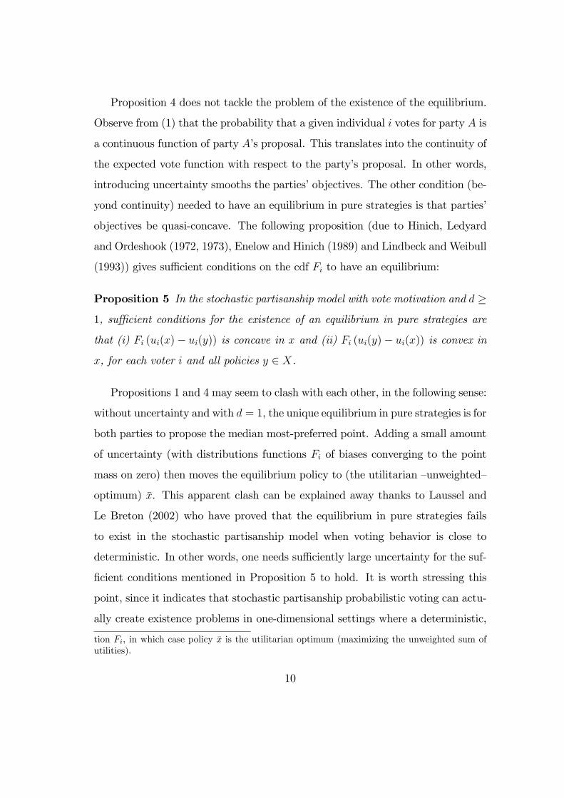
Proposition 4 does not tackle the problem of the existence of the equilibrium.

Observe from (1) that the probability that a given individual i votes for party A is

a continuous function of party A’s proposal. This translates into the continuity of

the expected vote function with respect to the party’s proposal. In other words,

introducing uncertainty smooths the parties’objectives. The other condition (be-

yond continuity) needed to have an equilibrium in pure strategies is that parties’

objectives be quasi-concave. The following proposition (due to Hinich, Ledyard

and Ordeshook (1972, 1973), Enelow and Hinich (1989) and Lindbeck and Weibull

(1993)) gives suffi cient conditions on the cdf Fi to have an equilibrium:

Proposition 5 In the stochastic partisanship model with vote motivation and d ≥

1, suffi cient conditions for the existence of an equilibrium in pure strategies are

that (i) Fi (ui(x)− ui(y)) is concave in x and (ii) Fi (ui(y)− ui(x)) is convex in

x, for each voter i and all policies y ∈ X.

Propositions 1 and 4 may seem to clash with each other, in the following sense:

without uncertainty and with d = 1, the unique equilibrium in pure strategies is for

both parties to propose the median most-preferred point. Adding a small amount

of uncertainty (with distributions functions Fi of biases converging to the point

mass on zero) then moves the equilibrium policy to (the utilitarian —unweighted—

optimum) x. This apparent clash can be explained away thanks to Laussel and

Le Breton (2002) who have proved that the equilibrium in pure strategies fails

to exist in the stochastic partisanship model when voting behavior is close to

deterministic. In other words, one needs suffi ciently large uncertainty for the suf-

ficient conditions mentioned in Proposition 5 to hold. It is worth stressing this

point, since it indicates that stochastic partisanship probabilistic voting can actu-

ally create existence problems in one-dimensional settings where a deterministic,

tion Fi, in which case policy x is the utilitarian optimum (maximizing the unweighted sum ofutilities).

10

Downsian equilibrium in pure strategies exists.

Thanks to the continuity of parties payoffs, an equilibrium in mixed strategies

exists with stochastic partisanship probabilistic models. Moreover, Banks and

Duggan (2005) show that the support of this equilibrium converges to the median

most-preferred policy when the amount of noise goes to zero. Finally, observe that

moving to a win motivation for parties makes the existence problem worse, in the

sense that the conditions enunciated in Proposition 5 are not suffi cient anymore to

guarantee existence of a Nash equilibrium in pure strategies (see Duggan, 2014).

In other words, it is even more diffi cult to generate quasi-concave payoff functions

for parties with a win motivation, compared to a vote motivation.

4.2 Applications

The stochastic partisanship modeling has proved very attractive and has been

used in many applications to specific policy dimensions. As Persson and Tabellini

mention in their 2000 textbook, the reason for this success is that “these models

have unique equilibria even when the policy conflict is multidimensional”(p59).

For instance, Persson and Tabellini (2000) apply this approach to the modeling of

special interest politics (chapter 7), alternative electoral rules (chapter 8), public

debt issued by partisan candidates (chapter 14), or where candidates care about

economic policies not because of their ideology, but because they want to appro-

priate rents for themselves (chapter 4). At the same time, this approach has not

been used to explain empirically the policy positions of political parties in actual

elections. Even for unidimensional policy, Persson and Tabellini (2000) write that

they “know of no attempts in the literature to try and discriminate empirically

between this model of electoral competition and the median voter model. (p58)”.

One reason for this lack of application is that the stochastic partisanship approach

predicts that both parties should converge to the same policy platforms. As we

11

will see later (see section 7.2), this prediction is not supported by the empirically

evidence. Moreover, it is worth recalling here Laussel and Le Breton (2000)’s

conclusion that “intrinsic preferences for candidates must be dispersed enough

across the electorate to make the first order approach [underlying Proposition 4]

valid (...). Hopefully the next wave of empirical structural models of electoral

competition will incorporate that aspect into the picture.”

Observe that, if the biases are independently distributed and if there is a

large number of voters, then there is no aggregate uncertainty, in the sense that,

thanks to the law of large numbers, the result of the election is deterministic when

both parties announce their policy platforms. In other words, we need either a

small number of voters, or correlated shocks, for aggregate uncertainty to occur

with probabilistic partisanship models. We now move to alternate modelling of

uncertainty on individual voting behavior, which generates aggregate uncertainty.

5 The stochastic preferences approach

An alternative way to introduce uncertainty is to assume that voters do not have

partisan preferences, as in the previous section, but rather that parties are uncer-

tain as to the policy preferences of voters.

5.1 Micro vs macro uncertainty over voters’preferences

There are two approaches to modelling the parties’uncertainty as to the voters’

policy preferences. The first starts at the individual voter level, and constructs

the expected vote/probability of winning functions of both parties by aggregating

voters’behaviors. The second models parties as having “macro level uncertainty”

as to the election results. We briefly describe a few examples of these two ap-

proaches, starting with the micro approach.

12

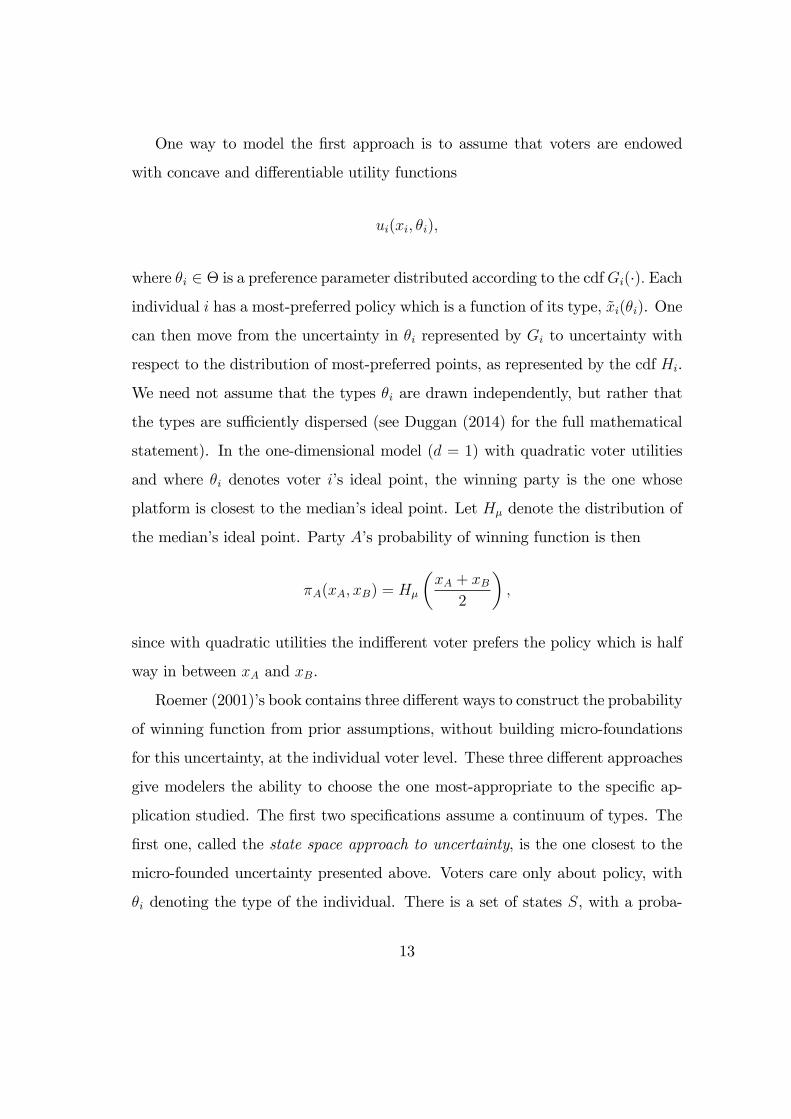
One way to model the first approach is to assume that voters are endowed

with concave and differentiable utility functions

ui(xi, θi),

where θi ∈ Θ is a preference parameter distributed according to the cdfGi(·). Each

individual i has a most-preferred policy which is a function of its type, xi(θi). One

can then move from the uncertainty in θi represented by Gi to uncertainty with

respect to the distribution of most-preferred points, as represented by the cdf Hi.

We need not assume that the types θi are drawn independently, but rather that

the types are suffi ciently dispersed (see Duggan (2014) for the full mathematical

statement). In the one-dimensional model (d = 1) with quadratic voter utilities

and where θi denotes voter i’s ideal point, the winning party is the one whose

platform is closest to the median’s ideal point. Let Hµ denote the distribution of

the median’s ideal point. Party A’s probability of winning function is then

πA(xA, xB) = Hµ

(xA + xB

2

),

since with quadratic utilities the indifferent voter prefers the policy which is half

way in between xA and xB.

Roemer (2001)’s book contains three different ways to construct the probability

of winning function from prior assumptions, without building micro-foundations

for this uncertainty, at the individual voter level. These three different approaches

give modelers the ability to choose the one most-appropriate to the specific ap-

plication studied. The first two specifications assume a continuum of types. The

first one, called the state space approach to uncertainty, is the one closest to the

micro-founded uncertainty presented above. Voters care only about policy, with

θi denoting the type of the individual. There is a set of states S, with a proba-

13

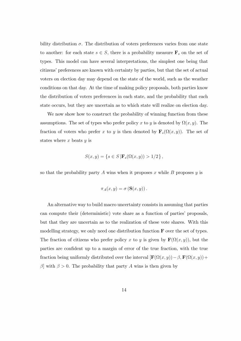
bility distribution σ. The distribution of voters preferences varies from one state

to another: for each state s ∈ S, there is a probability measure Fs on the set of

types. This model can have several interpretations, the simplest one being that

citizens’preferences are known with certainty by parties, but that the set of actual

voters on election day may depend on the state of the world, such as the weather

conditions on that day. At the time of making policy proposals, both parties know

the distribution of voters preferences in each state, and the probability that each

state occurs, but they are uncertain as to which state will realize on election day.

We now show how to construct the probability of winning function from these

assumptions. The set of types who prefer policy x to y is denoted by Ω(x, y). The

fraction of voters who prefer x to y is then denoted by Fs(Ω(x, y)). The set of

states where x beats y is

S(x, y) = s ∈ S |Fs(Ω(x, y)) > 1/2 ,

so that the probability party A wins when it proposes x while B proposes y is

πA(x, y) = σ (S(x, y)) .

An alternative way to build macro uncertainty consists in assuming that parties

can compute their (deterministic) vote share as a function of parties’proposals,

but that they are uncertain as to the realization of these vote shares. With this

modelling strategy, we only need one distribution function F over the set of types.

The fraction of citizens who prefer policy x to y is given by F(Ω(x, y)), but the

parties are confident up to a margin of error of the true fraction, with the true

fraction being uniformly distributed over the interval [F(Ω(x, y))−β,F(Ω(x, y))+

β] with β > 0. The probability that party A wins is then given by

14

πA(x, y) =

0 if F(Ω(x, y)) + β ≤ 1/2

F(Ω(x,y))+β−1/22β

if 1/2 ∈ [F(Ω(x, y))− β,F(Ω(x, y)) + β]

1 if F(Ω(x, y))− β ≥ 1/2

The easiest interpretation of this error-distribution model is that parties are con-

fident about pre-election polls results (the computed expected vote share) up to

a certain margin of confidence.

Finally, Roemer (2001) also proposes a finite type model of uncertainty, which

is more cumbersome to describe.

Observe that all variants of macro (and micro) uncertainty generate aggre-

gate uncertainty, with the expected electoral results being a random variable for

both parties when announcing their policy platforms. The main characteristic of

those approaches is that, unlike in the stochastic partisanship approach, both the

probability of winning and the vote share functions are discontinuous along the

diagonal—when a party crosses over the other one by proposing the same policy.

Despite this discontinuity, there is a unique equilibrium in the case of unidimen-

sional policy space, where both parties propose the same policy (see Duggan 2006a

for the vote motivation, and Calvert 1985 for the win motivation). We refer to

Duggan (2014) for a more complete examination of the solutions under those two

forms of electoral motivation, and we turn to the much more developed analysis

of this model under policy motivations.

5.2 Purely policy motivated parties

We first develop the analytical modelling, before moving to various applications.

15

5.2.1 Theory

A Nash equilibrium in pure strategies of this game is dubbed a Wittman equilib-

rium. The following proposition has been proved by in various guises by Wittman

(1983, 1990), Hansson and Stuart (1984), Calvert (1985) and Roemer (1994):

Proposition 6 In the stochastic preference model with policy motivations and

d ≥ 1, if (x∗A, x∗B) is an equilibrium, then the candidates do not locate at the same

policy position: x∗A 6= x∗B.

The intuition for this proposition resides in the aggregate uncertainty gener-

ated by the stochastic preferences model. At the time of announcing their plat-

forms, parties face a trade-off between increasing their probability of winning and

moving closer to their most-preferred policy. Since parties differ in their policy

preferences, they end up proposing different platforms. For instance, if d = 1 and

utilities are quadratic with xA < xB, we have that the equilibrium, if it exists, is

of the form xA < x∗A < x∗B < xB.

Calvert (1985) and Roemer (1994) further show that, if the policy space is

unidimensional (d = 1), the stochastic preferences model with policy motivation

gets close to Downsian, in the sense that the equilibrium policies (assuming equi-

librium existence) of both candidates converge to the median ideal policy as the

amount of noise added to the Downsian model goes to zero.

As for equilibrium existence, the good news is that the discontinuity of the

probability of winning function when both parties propose the same policy does

not translate into a discontinuous pay-off function. The intuition is that the

discontinuity in πj occurs when both parties propose the same policy, so that

the utility obtained by a party is anyway the same with both policies. On the

other hand, quasi-concavity of the pay-off function is not guaranteed, so one needs

additional assumptions for equilibrium existence. These assumptions are not very

16

strict in the case of a unidimensional policy space. For instance, Roemer (1997)

proves that a suffi cient condition for equilibrium existence if d = 1 in the micro-

founded model described in section 5.1 is that the distribution of the median

ideal points among citizens be log concave. Roemer (2001, section 3.4) provides

a suffi cient condition for the existence of an equilibrium in pure strategies with

d = 1 with the error-distribution model of uncertainty, and Roemer (1997) proves

a similar one for the state-space model. Unfortunately, these conditions are stated

in terms of the probability of winning function πj, rather than in terms of the

data of the model. Roemer (2001, p.68) concludes that “we find that in most

interesting examples Wittman equilibria exist, but a truly satisfactory general

existence theorem is not known.”

Suffi cient conditions for existence are more diffi cult to find when d > 1 and,

to the best of our knowledge, there is no general proof of existence for multi-

dimensional policy spaces. As for the micro approach to uncertainty, Duggan

(2014, p.43) states that “in higher dimensions, equilibria in the stochastic prefer-

ence model can fail to exist”, while Roemer (2001, p.163) writes that “all we can

say is that there is no guarantee that Wittman equilibrium exists when d > 1,

but if one does exist, it is probably generic.”

Finally, observe that equilibria in mixed strategies exist, and that they are

continuous from the Downs model (in the sense that the support of any mixed

strategies equilibrium converges to the Downsian outcome as the amount of noise

tends toward zero, see more in Duggan, 2014).

5.2.2 Applications

Roemer (2001)’s book contains many applications of this model to different policy

realms, where d = 1, including fiscal policy, partisan dogmatism and political

extremism, and political cycles. These models generate analytical predictions

17

which can then be taken to the data, or are solved using calibrated numerical

simulations. Another example of policy application can be found in De Donder

and Hindriks (2007), who study the political economy of social insurance with

voters’heterogeneity on two dimensions: income and risk levels. Individuals vote

over the extent of social insurance (d = 1), which they can complement on the

private market. They obtain equilibrium policy differentiation with the Left party

proposing more social insurance than the Right party (the Right party attracts

the less risky and richer individuals, and the Left party attracts the more risky

and poorer individuals). In equilibrium, each party is tied for winning. They also

attempt at calibrating the model with real data, using U.S. data from the Panel

Study of Income Dynamics survey.

Roemer (2001, chapter 5) goes further and endogenizes the policy preferences

Uj(x) of the political parties. He assumes that each party represents the set of

citizens who vote for it in equilibrium (which he calls the party’s membership).

Each party member receives an “equal weight”in the determination of party pref-

erences. He formalized this “equal weight”requirement in two different manners.

The first one, where each party represents its “average member”, can be applied

to multi-dimensional policy spaces, as we will see in section 5.3.2. The second

one can only be applied to unidimensional policy spaces, and assumes that party

members vote to elect their party representative, with this representative imposing

its preferences when competing electorally with the other party.

Finally, we are not aware of applications of the Wittman model to (i) multi-

dimensional policy spaces, and (ii) explaining the observed policy positions of

parties in past elections.

We now move to the case where parties care about both electoral and policy

considerations.

18

5.3 Party members: opportunists and militants

Parties are formed by individuals who may have different motives for being in

the party. In this section we first outline Roemer’s (2001) model in which there

are two party factions (the opportunists and the militants), then present some

applications of this model.

5.3.1 Theory

Roemer (2001) assumes that two factions coexist inside both political parties. In

each party j, the opportunists care exclusively about winning the elections (and

maximize πj(xj, xk), j 6= k), while the militants care about the specific policy pro-

posal x which their party proposes (and maximize Uj(x)). Any of the approaches

mentioned in section 5.1 above can be used to model aggregate uncertainty (so

that πj is not degenerate).

Both intra-party factions bargain with each other over the party’s policy pro-

posal. Each faction has a complete preference order on the set of possible policies,

and Roemer assumes that the party’s preference ordering is determined by the

intersection of these two orders. In other words, unanimity between the two fac-

tions is required for a party to accept a deviation from its current policy. This

unanimity rule determines the preferences (payoffs) of the two parties who simul-

taneously choose their political platforms. A party unanimity Nash equilibrium

(PUNE) is a equilibrium of this game.

Definition 7 Assume that two parties, denoted A and B, compete in an election.

The policy pair (xA, xB) is a PUNE if and only if ∀(j, k) ∈ A,B, j 6= k, @x ∈ X

such that (i) Uj(x) ≥ Uj(xj) and (ii) πj(x, xk) ≥ πj(xj, xk), with at least one

strict inequality.

Roemer does not provide a general existence theorem for the PUNEs, but men-

19

tions that PUNEs do exist in all the applications he has studied. The intuition for

why PUNEs exist (even in multidimensional policy spaces) is that the unanimity

requirement (between factions) restricts the set of admissible deviations for both

parties. Another way to put it is that the unanimity requirement means that each

party’s preference ordering over policies is incomplete, since a party can only rank

policies if both its factions have the same ordering. Since deviations must fulfill

the harsh requirement of pleasing both factions at the same time, the existence of

PUNEs in many environments becomes intuitive.

Roemer (2001) establishes that the PUNEs (when they exist) form a two-

dimensional manifold whatever the dimensionality of the policy space d ≥ 2. He

shows (Roemer 2001, section 8.3.) that the bargaining that takes place within

parties can be represented as a generalized Nash bargaining problem when ap-

propriate convexity properties hold. More precisely, take the threat point of this

intra-party bargaining game to be the situation which occurs when the other

party wins the election for sure. The Nash bargaining games between militants

and opportunists in party A and party B are given by

maxx∈X

[πA(x, xB)− 0]α [UA(x)− UA(xB)]1−α , and (3)

maxx∈X

[πB(xA, x)− 0]β [UB(x)− UB(xA)]1−β (4)

where α and β measure the relative bargaining power of the opportunists in party

A and B respectively.

Roemer (2001) shows that a PUNE can be expressed as a pair of policies

(xA, xB) which solves equations (3) and (4) simultaneously for some values of

α, β ∈ [0, 1]. The two-dimensional manifold of PUNEs can then be indexed by

these two variables, α and β. It is important to note that we cannot be guar-

anteed that an equilibrium will exist for any pre-specified pair of numbers α and

20

β. Roemer (2001) shows that the specific case where both factions have the same

bargaining power in both parties (α = β = 1/2) corresponds to the Wittman equi-

librium, while the classical Downsian equilibrium (with purely policy motivated

parties) corresponds to α = β = 1.

5.3.2 Applications

The PUNE modelling approach has been applied to many different policy areas.

In several applications, the model delivers neat analytical predictions which are

valid for all PUNEs. In that sense, the multiplicity of PUNEs does not prevent

from obtaining sharp analytical predictions as seen in the following two examples.

Roemer (1999) studies electoral competition over quadratic taxes, and obtains

that all PUNEs exhibit marginal tax rates which increase with income. This

provides a positive foundation for the observation that income tax schedules are

progressive in most developed countries. Roemer (1998) supposes that the elec-

torate is concerned with two issues (taxation and, say, religion) and shows, under

certain conditions (namely, that the salience of the religious issue is suffi ciently

large, that uncertainty is suffi ciently small, and that the mean income of the co-

hort of voters who hold the median religious view is greater than mean income in

the population as a whole) that, in all PUNEs, both parties propose a tax rate of

zero! This result illustrates starkly the importance of “non economic”preferences

in the democratic determination of the tax rates.

Lee and Roemer (2006) have applied this model to the race issue in the US, by

means of a calibration (for instance, the distribution of voter racism is estimated

from the American National Election Studies). They fit the model to the data

for every presidential election in the period 1976-92 and achieve an excellent fit.

Their objective goes beyond fitting observed electoral data, since it consists in

conducting counterfactual experiments looking at how the equilibrium tax rates

21

would be affected by variations in the racist preferences of the US electorate.

They obtain that “the marginal tax rate would increase by at least ten points,

were American voters not racist, making the US fiscal system much closer in size

to that of the northern European democracies. (Roemer 2006, p. 1026).

Another application is due to Cremer et al (2007) who study the PUNEs in

a model where both parties have to choose how much to tax a polluting good,

and the fraction of the tax proceeds to rebate based on the labor (as oppose to

capital) income of the constituents. They calibrate the model based on US data

(the polluting good being energy) and obtain two different sets of equilibria, one

with a tax on the polluting good and another with a subsidy.

Roemer (2001) extends the PUNE concept to the case where the militants’util-

ity is endogenous, and is given by the average utility among the party members

(defined, as in section 5.2.2, as the set of citizens who vote for this party at equi-

librium). Roemer (2001, chapter 13) develops two applications of this PUNEEP

(where the last two letters stand for “endogenous parties”). The first uses the Na-

tional Election Surveys to parametrize the preferences of the US polity when the

two-issue space consists of taxation and race. The second application endogenizes

parties in the model of progressive taxation mentioned above (Roemer, 2009).

While the PUNE approach has proved very fruitful in many applications to

specific policy areas, we are unaware of attempts to use this framework to replicate

generic policy positions of political parties in specific elections.

We have covered in section 4 above on stochastic partisanship the case where

voters disagree on the attractivity of exogenous, non-policy related characteristics

of political parties. The next section covers the case where they all agree that one

party has better characteristics than another.

22

6 Valence models

Stokes (1963, 1992) seminal papers emphasized that the non-policy evaluations,

or valences, of candidates by the electorate are just as important as electoral pol-

icy preferences. He was particularly concerned with the fact that the Downsian

and policy motivated models with and without uncertainty did not do well when

taken to the data and argued that this evidence should allow theorists to modify

their models. Stokes proposed that there exist “evaluative”dimensions that he

termed “valence issues”that are fundamentally different from any policy positions

the parties may have, and that moreover do not affect the distribution of parties

and voters. So that valence issues affect voters’electoral choices independent of

the policies chosen by candidates. In Stokes’world, voters share the same beliefs

over valence issues such as reducing crime, increasing economic growth, or evalua-

tions of candidates’characteristics such as integrity, charisma or competency. He

posited that candidates cannot affect voters’valence beliefs during the election,

i.e., that voters’valence issues are independent of policy and are non-manipulable

by candidates. He also argued that while valence issues are exogenously given

to candidates at election time, they may vary across candidates, e.g., voters may

perceive candidates as differing in ability to govern.

Stokes seminal papers led researchers to incorporate non-policy factors into

spatial models. We do not exhaustively cover all the valence models available

in the literature, rather we have chosen to pick different models illustrating the

variety of valence models available in the literature. We first study the case of a

unidimensional policy space before moving to multidimensional spaces.

23

6.1 Valence in unidimensional policy spaces

In this section, we assume that two parties compete electorally by simultaneously

choosing a policy in a one-dimensional policy space (d = 1). As in section 4, voters

care both for policies, and for the party which enacts those policies. Abusing

slightly notation, we have that

ui(x, j) =

ui(xA) + ϑA if j = A

ui(xD) + ϑD if j = D. (5)

Unlike in section 4, the non-policy preference parameters vA and vD are common to

all voters. These represent the valence of the parties, and without loss of generality

assume that ϑ = ϑA − ϑD > 0, so that party A (respectively, D) is valence-

advantaged (valence-disadvantaged), with ϑ measuring the relative valence of A

compared to D. So that voter i votes for party A if ui(xA)− ui(xD) + ϑ > 0.

Models with policy motivated parties where the electorate cares about both

policies and candidates’valence may generate policy divergence, even in the ab-

sence of uncertainty (which is not the case without valence, see above Section

3). For instance, assume that xA < xm < xD where xm is the median voter’s

blisspoint. Suppose that A has a valence advantage over D which is such that A

wins the election unless

|xA − xm| > |xD − xm|+ y,

where y > 0. In words, party A is guaranteed to win if it locates within y units of

the median, and thus can move closer to her ideal point xA than xm. For instance,

if xA < xm − y, there is an equilibrium with xD = xm and xA = xm − y, so that

A wins for sure and D prevents A from moving further to the left.

We now introduce uncertainty into the model. Two ways of adding uncertainty

24

have been studied in the literature: one over the electoral outcome, the other over

candidates’valence. While we do not exhaustively cover the literature, we now

summarize some of results derived from valence models with uncertainty.

6.1.1 Uncertainty over election results

In this section we assume that candidates don’t know the location of the median

voter but know the valence advantage of candidate A relative to D.

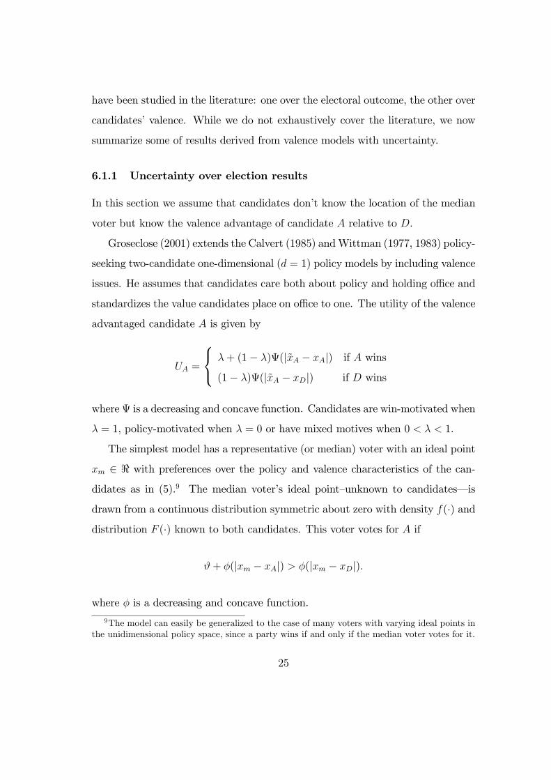
Groseclose (2001) extends the Calvert (1985) andWittman (1977, 1983) policy-

seeking two-candidate one-dimensional (d = 1) policy models by including valence

issues. He assumes that candidates care both about policy and holding offi ce and

standardizes the value candidates place on offi ce to one. The utility of the valence

advantaged candidate A is given by

UA =

λ+ (1− λ)Ψ(|xA − xA|) if A wins

(1− λ)Ψ(|xA − xD|) if D wins

whereΨ is a decreasing and concave function. Candidates are win-motivated when

λ = 1, policy-motivated when λ = 0 or have mixed motives when 0 < λ < 1.

The simplest model has a representative (or median) voter with an ideal point

xm ∈ < with preferences over the policy and valence characteristics of the can-

didates as in (5).9 The median voter’s ideal point—unknown to candidates– is

drawn from a continuous distribution symmetric about zero with density f(·) and

distribution F (·) known to both candidates. This voter votes for A if

ϑ+ φ(|xm − xA|) > φ(|xm − xD|).

where φ is a decreasing and concave function.

9The model can easily be generalized to the case of many voters with varying ideal points inthe unidimensional policy space, since a party wins if and only if the median voter votes for it.

25

When candidates care only about winning and there is no valence advantage,

i.e., λ = 1 and ϑ = 0, then Groseclose re-states Calvert’s (1985) result in Propo-

sition 8 (i) and shows in part (ii) that, with purely offi ce motivated parties, the

introduction of even an infinitesimal valence destroys equilibrium existence.

Proposition 8 (i)When λ = 1 and ϑ = 0. The unique equilibrium is x∗A = x∗D =

xm = 0. (ii) When λ = 1 and V > 0, there is no pure-strategy Nash equilibrium.

The intuition behind the non-existence result in Proposition 8 (ii) is simple.

While candidate A prefers to adopt the same policy as D to capitalize on its

valence advantage so as to win with certainty, D has to move away from A to have

even a small chance at winning. Hence, no matter what positions the candidates

adopt, at least one wants to move. This reasoning extends to the case of multi-

dimensional policy spaces (d > 1), and to the vote motivation objective. This

illustrates the knife-edge quality of the Downs and Wittman results when valence

is introduced. We refer the reader to the appendix for a brief survey of papers

dealing with Nash equilibria in mixed strategies in that setting.

Groseclose (2001) then focuses on the case where candidates care about policy

and offi ce (i.e., λ < 1), and where their ideals are symmetrically located about the

median voter’s expected ideal point, i.e., xA = −xD. He focuses on the symmetry

of bliss points essentially for analytical convenience and notes that this assumption

is reasonable when each party represents one half of the electorate, when parties’

most-preferred policies are the ideal points of their median members, and when

voters preferences are distributed symmetrically.

Groseclose (2001) does not provide any existence or uniqueness result, but

rather characterizes the equilibrium in pure strategies, assuming it exists. His

numerical results show the existence of at most one such equilibrium (but no

equilibrium when λ is large and V small, which is not surprising in the light of

Proposition 8). He obtains the following results.

26

Proposition 9 For very general forms of Ψ(·), φ(·) and f(·) the following six

relations hold (no proof is given of relation 5). (i) As A’s valence advantage

increases, divergence among candidates’ policies increases. (ii) As A’s valence

advantage increases from 0 to a small amount, A moves towards the expected me-

dian. (iii) However, as A’s advantage increases beyond a certain point, A adopts

a more extreme position closer to her ideal point. (iv) As A’s valence advantage

increases from 0 to a small positive amount, D moves away from the expected

median. (v) D’s equilibrium location moves away from the expected median as

A’s valence advantage increases. (vi) For all levels of A’s valence advantage, A’s

policy is more moderate than D’s.

The key characteristic of the modelling which explains those results is that

election uncertainty increases when parties diverge (at the opposite, when both

propose very similar policies, A is sure to win the election). The intuition for

results (ii) (dubbed the “moderating frontrunner”effect) and (iv) (the “extrem-

ist underdog” effect) is as follows. The equilibrium policy of a party trades-off

centripetal incentives (moving closer to the center to increase its probability of

winning) and centrifugal incentives (moving away from the center to increase its

utility in case of a win). Increasing A’s valence advantage from zero moves the

cut-point voter (the one indifferent between both parties) further away from A’s

policy, and closer to D’s policy. If the voters’utilities are concave enough, this

means that the (absolute value of the) marginal utility of the cut-point voter in-

creases at the policy proposed by A, and decreases at the policy proposed by D.

This reinforces the centripetal force for A, and decreases it for D, resulting in

both parties moving in the direction of D’s ideal policy.10

10Adams, Merrill and Grofman (AMG, 2005, chapter 11) stress that the extremist underdogeffect requires a level of uncertainty over the location of the median voter which is not empiricallyreasonable, at least in US elections (see section 7.3). Note that AMG (2005) assume that votershave quadratic preferences, while Groseclose’s suffi cient condition for the extreme underdog

27

Part (3) of Proposition 9 is proved by showing that, when its valence advantage

becomes infinite, party A locates at its preferred policy xA and wins for sure.

Beyond proving part (6), Groseclose also proves the counter-intuitive result that

if party A has a large valence advantage then party D may propose at equilibrium

a policy which is more extreme than its blisspoint xD! The intuition is that, when

ϑ is large, the cut-point voter is located at a more extreme position than D’s

proposed policy (even when D proposes its favored policy xD). In that case, D

has an incentive to propose a more extreme position, trading off a first-order gain

in winning probability for a second-order loss in utility in case it wins the election.

As Groseclose (2001) writes “relations 2, 4, 5 and 6 [in Proposition 9] are

somewhat unintuitive, since instead, one might expect that valence-advantaged

candidates would parlay their advantage into a position that they personally fa-

vor more and disadvantaged candidates would do the opposite. However, notwith-

standing this, the results have strong empirical support. First, they are consistent

with Fiorina’s (1973) evidence against the marginality hypothesis.(...) Fiorina

finds—despite the conventional wisdom of congressional scholars of the 1950s and

1960s—that electorally strong incumbents tend to moderate more than electorally

weak incumbents.” (p 874). Ansolabehere, Snyder and Stewart (2001) also find

empirically that high-quality US House candidates adopt more moderate positions

than low-quality ones.

We now move to the case where the uncertainty pertains to the valence ad-

vantage of candidates, rather than directly to the elections results.

6.1.2 Uncertainty over valence

Londregan and Romer (1993) develop a two-party valence model of congressional

elections in which parties are represented by candidates at the constituency level.

effect to appear is that voters preferences are more concave than in the quadratic case (with anegative third derivative).

28

Candidates have divergent preferences over the unidimensional (d = 1) policy

space and differ in their ability to deliver constituency services, with abilities,

αA and αD, drawn independently of each other from a joint density function

φ(αA, αD) > 0 with cumulative density Φ(αA, αD). Let α ≡ (αA, αD) denote the

vector of abilities. Voters prefer candidates with higher abilities who can deliver

higher constituency services.

While parties only have noisy signals about candidates’abilities at the candi-

date selection stage, candidates abilities are perfectly known to voters at election

time. Parties are then unsure as to the electoral outcome when choosing their

platforms as they do so before voters’observe candidates’abilities.

At the beginning of the game, each party observes a signal of candidates’ability

and selects one candidate to represent it in the election with the party’s policy

being that of the chosen candidate. Let (xA, xD) denote the parties’platforms.

With a continuum of voters whose preferences satisfy the single crossing condi-

tion, the election is determined by the choice of the median voter. Parties’know

the location of the median voter’s ideal point and know that the post-election

constituency services provided by the winning candidate depends on her ability.

Given platforms, (xA, xD), the median voter’s utility, after observing candi-

dates’abilities, is given by

um(xj, j) = −d(xm, xj) + γϑ(αj),

where γ measures the importance voters give to the constituency services and

ϑ(αj)—an increasing function in αj—denotes the constituency services provided

by candidate j. Since ϑ(αj) is the same across voters and is independent of

candidates’policies, it fits our definition of valence, except that in this model ϑj

increases in candidate j’s ability.

29

The median voter votes for A when um(xA, A) > um(xD, D), i.e., when

ϑ(αA, αD) ≡ ϑA(αA)− ϑD(αD) >1

γ[d(xm, xA)− d(xm, xD)] .

So that the median votes for A when the valence gap between A andD, ϑ(αA, αD),

is large enough. Since at the platform selection stage parties view ϑ(αA, αD) as a

random variable, the ex-ante probability that A wins the election is given by the

probability that the median votes for A, i.e.,

πA(xA, xB;α) = Pr [um(xA, A) > um(xD, D)]

= Pr

[ϑ(αA, αD) >

1

γ[d(xm, xA)− d(xm, xD)]

]

where d(xm, xj) for j = A,D measures the distance between the median voter’s

ideal, xm, and the party’s policy xj.

For each pair of policy platforms (xA, xD) and each pair of median voter pref-

erences (xm, γ), there is a valence gap ϑ(αA, αD) that leaves the median voter

indifferent between voting for either candidate.

Candidate j’s expected utility, after the two parties have chosen their candi-

dates but before abilities are revealed, is given by

Uj(xA, xD) = −πA(xA, xB;α)d(xj, xA)− [1− πA(xA, xB;α)]d(xj, xD)

where d(xj, xA) and d(xj, xD) measure the distance between candidate j’s policy

and the policy implemented by the wining candidate. Candidates, who are policy

motivated, choose their policy platforms to maximize their expected utility.

Londregan and Romer (1993) prove the following proposition:

Proposition 10 (i) There is no pure strategy Nash equilibrium in which candi-

dates adopt the same platform, i.e., x∗A 6= x∗D. (ii) Moreover, x∗A and x

∗D will lie

30

outside an interval that contains the median voter’s ideal policy with this interval

increasing as γ increases.

Proposition 10 (i) says that the party’s equilibrium policies diverge. This

divergence is generated by divergence in the party’s policy preferences, by the

uncertainty parties have on candidates’abilities and by the trade-off voters face

between policies and the ability of candidates to deliver better constituency ser-

vices. Proposition 10 (ii) says that as γ increases, so that voters become more

service-motivated, policy polarization increases and policies become more extreme.

Intuitively, given the distribution of abilities, as γ increases, parties become more

uncertain about the level of constituency services candidates will provide to vot-

ers and so become more uncertain about how voters evaluate candidates. Thus,

Proposition 10 provides a minimum bound of the valence advantage that A must

have over D for there to be an equilibrium and shows that the bound increases as

voters give greater importance to valence issues.

The one testable hypotheses emanating from their model is that policy po-

larization increases in the saliency voters place on constituency services. Their

empirical tests find no support for this hypothesis in the 1978 US National con-

gressional election perhaps due to the small number of open seats in the election.

Adams, Merrill and Grofman (2005, chapter 11.3) propose a similar but simpler

model, where the valence advantage of party A is ϑ = v + ε, with v the expected

valance advantage, and where ε is distributed according to a normal distribution

with mean zero and standard deviation σv. They first show that, if an equilibrium

in pure strategies exists with v = 0, xA = −xD and x∗A = −x∗D, then there is

substantial candidate divergence. They then compute numerically the equilibrium

with v > 0. They obtain that the divergence between parties increases with both

v and σv. Moreover, both x∗A and x∗D shift to the left (closer to xA) when v

increases. This is in stark contrast with the results from the preceding section.

31

Results remain qualitatively similar when parties have mixed (policy and electoral)

motivation, rather than being purely policy-motivated.

6.2 Valence in multidimensional policy spaces

We now present multidimensional spatial competition models in which voters

also rank candidates along a valence dimension. These valence models derive the

conditions under which a d-dimensional party positioning equilibrium exists even

when the necessary conditions for a Condorcet winner do not hold. This is in

sharp contrast with the generic non-existence results in multidimensional models

without valence described in Proposition 2 .

6.2.1 Ansolabehere and Snyder’s win-seeking policy-valence model

In their multidimensional two-candidate valence model, Ansolabehere and Snyder

(2000) present the necessary and suffi cient conditions for existence of equilibrium

and characterize the equilibria when candidates care only about winning offi ce

in a model with no uncertainty except for ties broken in a fair manner. As An-

solabehere and Snyder state: when one candidate has a large enough valence

advantage that candidate wins the election irrespective of candidates’positions,

meaning that equilibria in multidimensional policy spaces with valence always

exist. Their contribution to this literature is to show that the “yolk,”11 which

sets limits on the uncovered set (McKelvey 1986; Cox 1987), bounds the set of

equilibria in these valence models.

Given voters’valences (ϑA, ϑD), offi ce-seeking candidates A and D simultane-

ously choose their policies xA and xB to maximize their expected payoff,

11The “yolk”is usually a small, centrally located set (McKelvey, 1986; Feld et al, 1988).

32

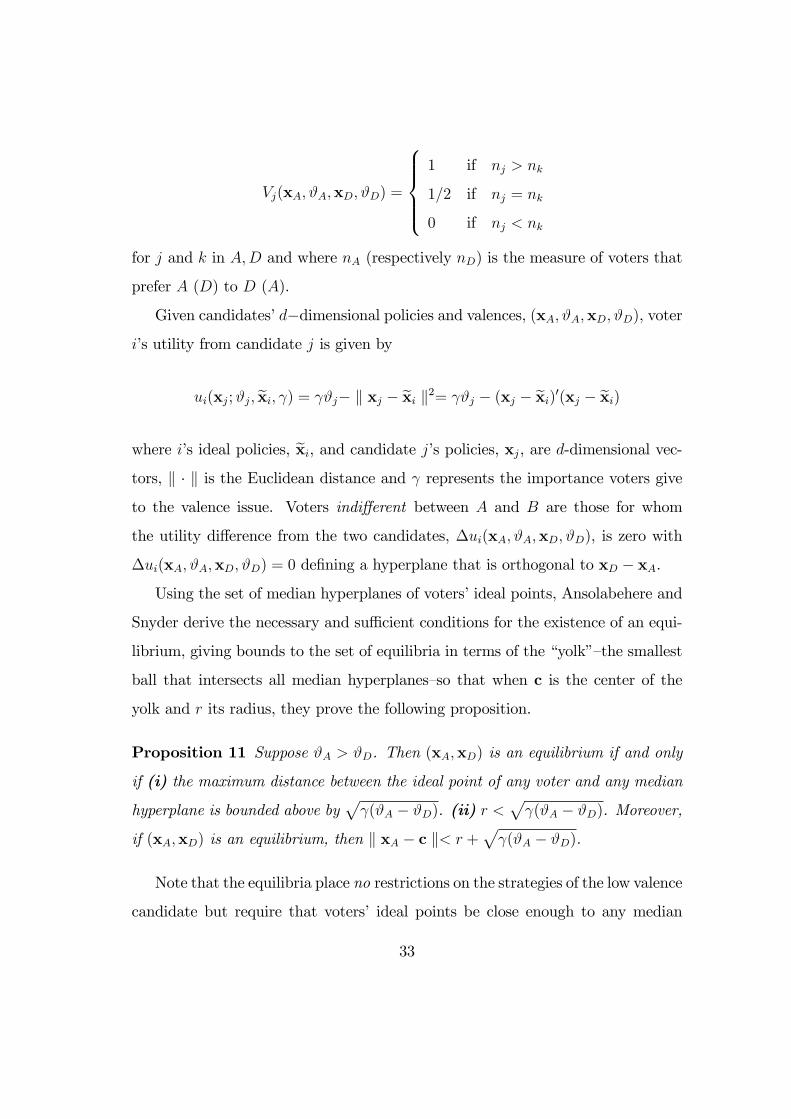
Vj(xA, ϑA,xD, ϑD) =

1 if nj > nk

1/2 if nj = nk

0 if nj < nk

for j and k in A,D and where nA (respectively nD) is the measure of voters that

prefer A (D) to D (A).

Given candidates’d−dimensional policies and valences, (xA, ϑA,xD, ϑD), voter

i’s utility from candidate j is given by

ui(xj;ϑj, xi, γ) = γϑj− ‖ xj − xi ‖2= γϑj − (xj − xi)′(xj − xi)

where i’s ideal policies, xi, and candidate j’s policies, xj, are d-dimensional vec-

tors, ‖ · ‖ is the Euclidean distance and γ represents the importance voters give

to the valence issue. Voters indifferent between A and B are those for whom

the utility difference from the two candidates, ∆ui(xA, ϑA,xD, ϑD), is zero with

∆ui(xA, ϑA,xD, ϑD) = 0 defining a hyperplane that is orthogonal to xD − xA.

Using the set of median hyperplanes of voters’ideal points, Ansolabehere and

Snyder derive the necessary and suffi cient conditions for the existence of an equi-

librium, giving bounds to the set of equilibria in terms of the “yolk”—the smallest

ball that intersects all median hyperplanes—so that when c is the center of the

yolk and r its radius, they prove the following proposition.

Proposition 11 Suppose ϑA > ϑD. Then (xA,xD) is an equilibrium if and only

if (i) the maximum distance between the ideal point of any voter and any median

hyperplane is bounded above by√γ(ϑA − ϑD). (ii) r <

√γ(ϑA − ϑD). Moreover,

if (xA,xD) is an equilibrium, then ‖ xA − c ‖< r +√γ(ϑA − ϑD).

Note that the equilibria place no restrictions on the strategies of the low valence

candidate but require that voters’ ideal points be close enough to any median

33

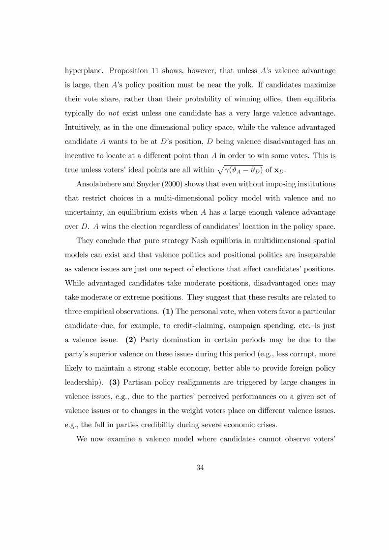
hyperplane. Proposition 11 shows, however, that unless A’s valence advantage

is large, then A’s policy position must be near the yolk. If candidates maximize

their vote share, rather than their probability of winning offi ce, then equilibria

typically do not exist unless one candidate has a very large valence advantage.

Intuitively, as in the one dimensional policy space, while the valence advantaged

candidate A wants to be at D’s position, D being valence disadvantaged has an

incentive to locate at a different point than A in order to win some votes. This is

true unless voters’ideal points are all within√γ(ϑA − ϑD) of xD.

Ansolabehere and Snyder (2000) shows that even without imposing institutions

that restrict choices in a multi-dimensional policy model with valence and no

uncertainty, an equilibrium exists when A has a large enough valence advantage

over D. A wins the election regardless of candidates’location in the policy space.

They conclude that pure strategy Nash equilibria in multidimensional spatial

models can exist and that valence politics and positional politics are inseparable

as valence issues are just one aspect of elections that affect candidates’positions.

While advantaged candidates take moderate positions, disadvantaged ones may

take moderate or extreme positions. They suggest that these results are related to

three empirical observations. (1)The personal vote, when voters favor a particular

candidate—due, for example, to credit-claiming, campaign spending, etc.—is just

a valence issue. (2) Party domination in certain periods may be due to the

party’s superior valence on these issues during this period (e.g., less corrupt, more

likely to maintain a strong stable economy, better able to provide foreign policy

leadership). (3) Partisan policy realignments are triggered by large changes in

valence issues, e.g., due to the parties’perceived performances on a given set of

valence issues or to changes in the weight voters place on different valence issues.

e.g., the fall in parties credibility during severe economic crises.

We now examine a valence model where candidates cannot observe voters’

34

individual valences and so are uncertain as to the electoral outcome.

6.2.2 Schofield’s win-seeking policy-valence model

Schofield (2007) introduces valence asymmetries among candidates into a mul-

tidimensional multi-candidate model where candidates choose their policies to

maximize their vote shares. Given the on-going debate about whether candidates

converge or not to the electoral mean12 in many electoral systems (e.g., US, and

many European countries), Schofield’s model studies the conditions under which

candidates converge to the electoral mean.

Candidates j ∈ C = 1, 2, ..., c simultaneously announce the d-dimensional

policies xj ∈ X before the election, with x = (x1, .,xj, ..,xc) denoting the matrix

of candidates’policies.

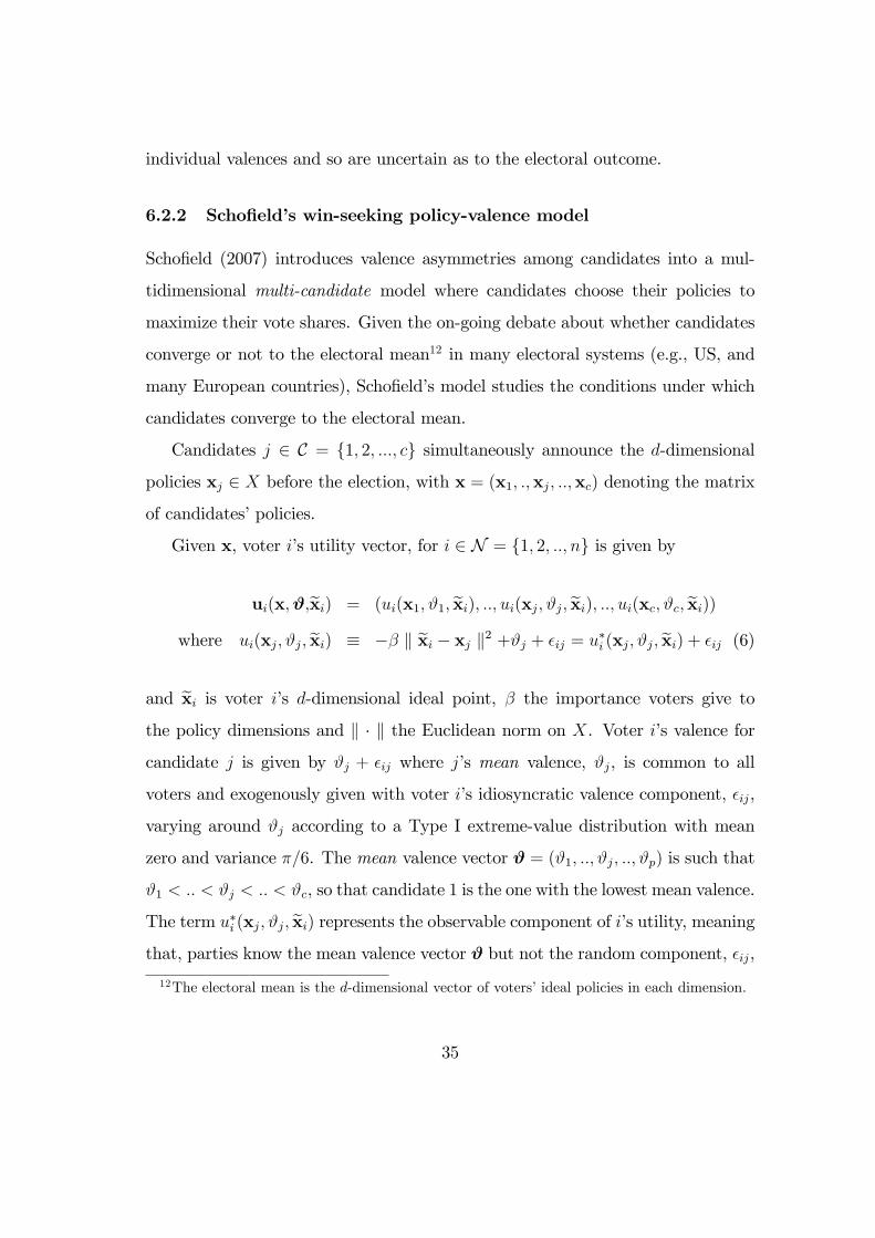
Given x, voter i’s utility vector, for i ∈ N = 1, 2, .., n is given by

ui(x,ϑ,xi) = (ui(x1, ϑ1, xi), .., ui(xj, ϑj, xi), .., ui(xc, ϑc, xi))

where ui(xj, ϑj, xi) ≡ −β ‖ xi − xj ‖2 +ϑj + εij = u∗i (xj, ϑj, xi) + εij (6)

and xi is voter i’s d-dimensional ideal point, β the importance voters give to

the policy dimensions and ‖ · ‖ the Euclidean norm on X. Voter i’s valence for

candidate j is given by ϑj + εij where j’s mean valence, ϑj, is common to all

voters and exogenously given with voter i’s idiosyncratic valence component, εij,

varying around ϑj according to a Type I extreme-value distribution with mean

zero and variance π/6. The mean valence vector ϑ = (ϑ1, .., ϑj, .., ϑp) is such that

ϑ1 < .. < ϑj < .. < ϑc, so that candidate 1 is the one with the lowest mean valence.

The term u∗i (xj, ϑj, xi) represents the observable component of i’s utility, meaning

that, parties know the mean valence vector ϑ but not the random component, εij,

12The electoral mean is the d-dimensional vector of voters’ideal policies in each dimension.

35

in voters’utility and so are unsure about the electoral outcome.

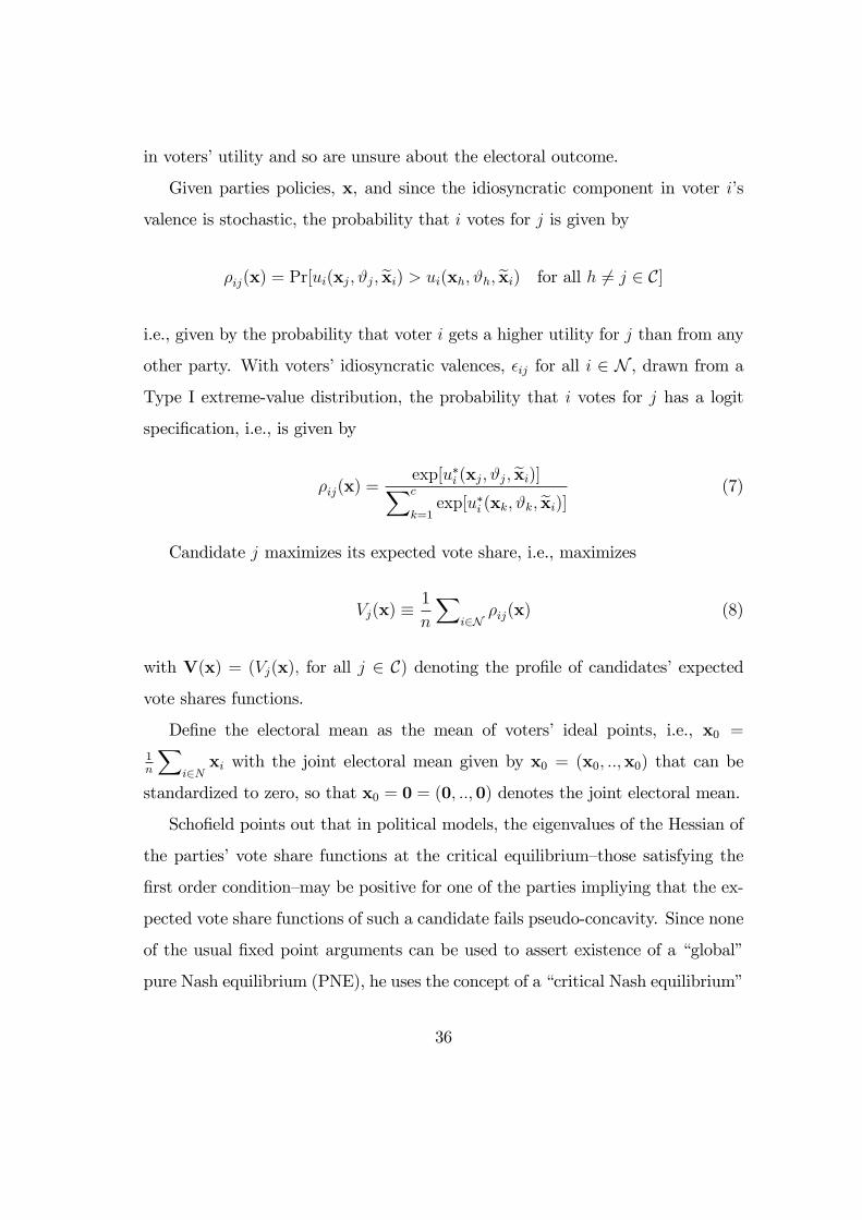
Given parties policies, x, and since the idiosyncratic component in voter i’s

valence is stochastic, the probability that i votes for j is given by

ρij(x) = Pr[ui(xj, ϑj, xi) > ui(xh, ϑh, xi) for all h 6= j ∈ C]

i.e., given by the probability that voter i gets a higher utility for j than from any

other party. With voters’idiosyncratic valences, εij for all i ∈ N , drawn from a

Type I extreme-value distribution, the probability that i votes for j has a logit

specification, i.e., is given by

ρij(x) =exp[u∗i (xj, ϑj, xi)]∑c

k=1exp[u∗i (xk, ϑk, xi)]

(7)

Candidate j maximizes its expected vote share, i.e., maximizes

Vj(x) ≡ 1

n

∑i∈N

ρij(x) (8)

with V(x) = (Vj(x), for all j ∈ C) denoting the profile of candidates’expected

vote shares functions.

Define the electoral mean as the mean of voters’ ideal points, i.e., x0 =

1n

∑i∈N

xi with the joint electoral mean given by x0 = (x0, ..,x0) that can be

standardized to zero, so that x0 = 0 = (0, ..,0) denotes the joint electoral mean.

Schofield points out that in political models, the eigenvalues of the Hessian of

the parties’vote share functions at the critical equilibrium—those satisfying the

first order condition—may be positive for one of the parties impliying that the ex-

pected vote share functions of such a candidate fails pseudo-concavity. Since none

of the usual fixed point arguments can be used to assert existence of a “global”

pure Nash equilibrium (PNE), he uses the concept of a “critical Nash equilibrium”

36

(CNE), namely a vector of strategies which satisfies the first-order condition for

a local maximum of candidates’expected vote share functions. Moreover, as he

points out standard arguments based on the index, together with transversality

arguments can be used to show that a CNE will exist and that, generically, it will

be isolated. A local Nash equilibrium (LNE) satisfies the first-order condition,

together with the second-order condition that the Hessians of all candidates are

negative (semi-) definite at the CNE. Clearly, the set of LNE will contain the PNE.

The suffi cient (necessary) condition for parties to converge to the electoral mean

is that the eigenvalues of the Hessian of second order partial derivatives of can-

didates’vote share functions, when evaluated at the electoral mean, be negative

(semi-)definite. Schofield shows that the necessary and suffi cient condition can be

summarized in what he calls the convergence coeffi cient that we now define.

Definition 12 Suppose all parties locate at the electoral mean, x0. The probability

that voters choose party 1, ρ1, with the lowest valence, using (7), is given by

ρ1(x0,ϑ) =[∑c

k=1exp[ϑk − ϑ1]

]−1

(9)

and the convergence coeffi cient of the election, c(ϑ, β, σ2), by

c(ϑ, β, σ2) ≡ 2β(1− 2ρ1)σ2, (10)

where ρ1(x0,ϑ) is given by (9) and σ2 ≡∑d

s=1var(s) denotes the sum of the

variance of voters’ideal points along each dimension with var(s) being the variance

of voters’ideal points along dimension s.

If parties locate at x0, ρ1(x0,ϑ) in (9) depends only on the valence advantage

that the top c− 1 candidates have over the lowest valence candidate, candidate 1,

is independent of candidates’policies and voters’ideal points, so is the same for

37

all voters and gives candidate 1’s expected vote share at x0.

Schofield (2007) proves the following Proposition.

Proposition 13 Let voter i’s idiosyncratic valence, εij for all i ∈ N , follow a

Type I extreme-value distribution. (i) The joint electoral mean, x0 satisfies the

first order conditions. (ii) The necessary and suffi cient condition for x0 to be a

LNE is that the matrix 2β(1−2ρ1)∇ has negative eigenvalues where ∇ is the d×d

variance-covariance matrix of voters’ ideal points. (iii) When the convergence

coeffi cient is smaller than the dimension of the policy space, i.e., c(ϑ, β, σ2) 6 d,

the necessary condition for convergence to x0 has been met by all parties. The

joint electoral mean, x0, is a LNE of the election. (iv) If c(ϑ, β, σ2) > d, the

necessary condition for convergence to x0 has not been met by at least one party.

The joint electoral mean, x0, is not a LNE of the election and at least one party

locates far from the electoral mean. (v) If d = 2 and c(ϑ, β, σ2) 6 1, the suffi cient

condition for convergence to x0 is met by all parties and the joint electoral mean,

x0, is LNE of the election.

Proposition 13 predicts that if an equilibrium exists at the electoral mean, all

parties adopt the same position, the electoral mean, i.e., candidates’equilibrium

policies are the mean of voters’ideal policies. The proposition also highlights that

when candidates’differ in their valences, an equilibrium in which all candidates

convergence to, or locate at, the electoral mean exists when c(ϑ, β, σ2) < d. The

convergence coeffi cient, c(ϑ, β, σ2) in (10), increases in β and σ2 and decreases

in ρ1. In particular, when the valence advantage of the top c − 1 candidates

increases relative to that of the most valence disadvantaged candidate, candidate

1, i.e., when the difference between ϑ1 and ϑ2, ϑ3, .., ϑc increases, the probability

voters choose candidate 1 with the lowest valence when located at the electoral

mean, ρ1(x0,ϑ) in (9), decreases. As a consequence, candidate 1 will move away

38

from the electoral mean x0 in order to increase its vote share, i.e., at x0 candidate

1’s vote share is at a minimum or at a saddle point. This result says that as

the valence advantage of the top c − 1 candidates relative to the most valence

disadvantaged candidate increases, the join electoral mean is less likely to be a

LNE of the election.

Note that c(ϑ, β, σ2) in (10) decreases when β decreases, i.e., when voters

give greater relative importance to the valence issue. It is then more likely that

c(ϑ, β, σ2) will be less than d, and thus more likely that all parties, including the

lowest valence party, adopt the same policies by locating at the electoral mean.

Thus, the greater the importance given to the valence issue the more likely it is

that candidates converge to the electoral mean, ceteris paribus.

Schofield’s (2007) result deals with more than two candidates and highlights

that existence of an equilibrium at the electoral mean depends on candidates’va-

lences, on the importance voters give to policies (and indirectly to the importance

voters give to the valence issue) and on how dispersed voters are in the policy

space. Schofield’s result is similar to that of Ansolabehere and Snyder (2000)

given in Proposition 11 when candidates have policy rather than win-motivation

and contrasts with the non-existence results in the non-valence multidimensional

models given in Proposition 2 in Section 3. In addition, Schofield’s results also

points out that convergence to the electoral mean depends on the probability

that voters’chose the candidate with the lowest valence. When c(ϑ, β, σ2) > d,

Proposition 13 says that parties locate away from the electoral origin.

6.2.3 Theoretical extensions of Schofield’s (2007) model

Schofield’s (2007) model has been extended to examine parties’equilibrium poli-

cies when voters in different regions of the country face different sets of parties

while allowing voters to have sociodemographic valences, i.e., allowing voters’

39

propensities to vote for the various candidates to depend on their sociodemo-

graphic characteristics (age, gender, education,...). Gallego et al (2014) develop a

model with national and regional parties. In the model, one party runs only in one

region (e.g., the Bloc Quebecois in Quebec) with national parties competing in all

regions to study the effect that this regional party has on the electoral outcome

in that region and on the national parties’positions in that region and in the rest

of the country. Labzina and Schofield (2015) adapt this regional model to study

a country with three regions in which there are two regional parties competing

in two different regions and three national parties competing in all regions. In

these regional models, voters’utilities depend on the region in which they live

and the parties competing in that region. The conditions for convergence to the

regional electoral mean are similar to those in Schofield (2007) given in Section

6.2.2, convergence at the national level requires convergence in every region.

Gallego and Schofield (2016a) extend Schofield’s (2007) model to study the

effect that advertising has on the policy position of US Presidential candidates.

Voters are charactretized by their policy preferences and by their campaign toler-

ance level—the number of times they want to be contacted by candidates—and by

three exogenously given valences: sociodemographic (age, income, etc.) and com-

petency valences as well as by candidates’traits valences (candidates’charisma,

age, race, etc.). The model shows that in spite of the fact that the one-person-

one-vote principle applies, candidates weight voters differently in their policy and

advertising campaigns, giving higher weights to undecided voters and little or no

weight to voters who vote with high probability for any candidate. Moreover, like

in Schofield’s (2007) model, the valence advantage of the top c − 1 candidates

relative to the lowest valence candidate affects convergence to voters’weighted

mean policy and campaign tolerance levels.

Gallego and Schofield (2016b) extend the Gallego and Schofield (2016a) model

40

to examine the effect that campaign advertising has on the policy positions in US

Presidential elections at both the state and the national levels when differences

across states matter. Candidates’electoral campaign consists of their policy and

advertising campaign in each state and at the national level. Voters’utility func-

tion depend on candidates campaign in their state of residence and at the national

level as well as on their sociodemographic, traits and competency valences with

valences having an idiosyncratic component, unobserved by candidates, drawn

from Type-I Extreme Value distributions. Convergence to the state weighted pol-

icy and campaign tolerance mean depends on the combined valence advantage of

the top c − 1 candidates relative to the lowest valence candidate in that state

and national levels. Candidates’electoral state campaigns determine the electoral

campaign at the national level so that, convergence at the national level depends

on convergence in each state. If candidates converege to the weighted state and

national means, they weight undecided states more heavily than states voting

with high probability for any candidate. Thus, providing a theoretical foundation

for candidates spending more time and resources during the electoral campaign

in undecided states and shows the effect that the combined state and national

valences have on convergence at the state and national levels.

6.2.4 Endogeneizing valence: political activists in Schofield (2007)

Even though published earlier, Schofield’s (2006) extends Schofield’s (2007) multi-

dimensional multi-candidate model by allowing candidates to have both exogenous

and endogenous valences. The endogenous valence is generated by the contribu-

tions (of time and money) party activists make to candidates to influence their

policy positions with candidates using these resources to present themselves more

effectively to voters thus increasing their endogenous valence. Since activists have

more extreme positions than average voters, candidates must trade-off adopt-

41

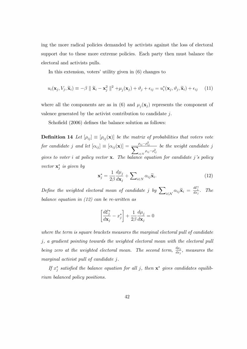
ing the more radical policies demanded by activists against the loss of electoral

support due to these more extreme policies. Each party then must balance the

electoral and activists pulls.

In this extension, voters’utility given in (6) changes to

ui(xj, Vj, xi) ≡ −β ‖ xi − x2j ‖2 +µj(xj) + ϑj + εij = u∗i (xj, ϑj, xi) + εij (11)

where all the components are as in (6) and µj(xj) represents the component of

valence generated by the activist contribution to candidate j.

Schofield (2006) defines the balance solution as follows:

Definition 14 Let [ρij] ≡ [ρij(x)] be the matrix of probabilities that voters vote

for candidate j and let [αij] ≡ [αij(x)] =ρij−ρ2ij∑i∈N

ρij−ρ2ijbe the weight candidate j

gives to voter i at policy vector x. The balance equation for candidate j’s policy

vector x∗j is given by

x∗j =1

2β

dµjdxj

+∑

i∈Nαijxi. (12)

Define the weighted electoral mean of candidate j by∑

i∈Nαijxi =

dE∗jdxj. The

balance equation in (12) can be re-written as

[dE∗jdxj− x∗j

]+

1

2β

dµjdxj

= 0

where the term is square brackets measures the marginal electoral pull of candidate

j, a gradient pointing towards the weighted electoral mean with the electoral pull

being zero at the weighted electoral mean. The second term,dµjdxj, measures the

marginal activist pull of candidate j.

If x∗j satisfied the balance equation for all j, then x∗ gives candidates equilib-

rium balanced policy positions.

42

Note that if µj(zj) = 0 for all j ∈ C, then we are back in Schofield’s (2007)

exogenous valence model. Schofield (2006) proves the following proposition.

Proposition 15 Let the stochastic valence component in voters’utility function

in (11) have a Type I extreme-value distribution in the model with exogenous and

activist valences. (i) The first order condition for x∗ to be an local strict Nash

Equilibrium is that it is a balance solution. (ii) If all activist valence functions

are highly concave, in the sense of having negative eigenvalues of suffi ciently great

magnitude, the balance solution will be a Pure Nash Equilibrium of the election.

Schofield’s (2006) endogenous valence model highlights that if the activists

valence functions are suffi ciently concave, there exists a strict LNE in which d-

dimensional policies balancing the activist and electoral pulls. With their re-

sources activist pull policies away from the electoral mean by providing resources

that candidates’use to increase their endogenous valence.

We now discuss empirical applications of Schofield’s (2007) valence models.

6.2.5 Empirical applications of Schofield-type valence models

The empirical literature provides substantial evidence that valence components

contribute in a significant way to an understanding of voter choice. For example,

Clarke, Kornberg and Scotto (2009) and Clarke, Sanders, Stewart and Whiteley

(2005), Clarke, Scotto and Kornberg (2011) and Clarke, Kornberg, MacLeod and

Scotto (2005) study the effect that electoral perceptions of leaders’character traits

have on British, Canadian and US elections. From their analysis for Britain, they

conclude that electoral responses

“... were a reflection largely of [the] changing perceptions of the

decision-making competence of the main political parties and their

43

leaders. At any point in time, [the] preferences were strongly influ-

enced by their perceptions of the capacity of the rival parties– the

putative alternative governments of the day– to solve the major pol-

icy problems facing the country.”

Thus, valence—as measured by voters’perceptions of the candidates’or party

leaders’ character traits—matter in electoral outcomes. Clarke, Kornberg and

Scotto (2009: 159) test the “Downsian” or pure spatial stochastic model and

a traits model of the 2000 and 2004 US presidential elections and conclude that

“the two models have approximately equal explanatory power.”

Taking this evidence seriously, Schofield and co-authors used his 2007 model

to study elections in developed and developing countries under various political

regimes (presidential, parliamentary and anocratic13). The advantage of using

Schofield’s (2007) model to study actual elections is that the model assumes that

voters’idiosyncratic valence components come from Type-I Extreme value distri-

butions. The probability that a voter chooses any party has a Logit specification

and provides an easy transition to using empirical multinomial Logit (MNL) mod-

els to estimate the coeffi cients in voter i’s utility functions in (6) in real elections.

In order to find if there is an equilibrium at the electoral mean x0 in a particular

election, party j’s expected vote share function in (8) at x0 must be estimated

and this requires estimating the probability that voter i chooses candidate j in

(7) in the election. Estimating this probability requires finding estimates of the

components in voter i’s utility in (6): the importance voters give to the policy

dimension, β, voter i’s ideal policy, xi, party j’s policy position, xj, and j’s

13In anocracies, a dictator governs alongside a legislature but exerts undue influence on theelection. Anocracies lack important democratic institutions such as freedom of the press. Sinceautocrats hold regular elections in an attempt to give their regime legitimacy, anocracies are alsocalled partial-democracies. Opposition parties participate in elections to become known politicalentities and to communicate with voters. Even though their objective is to oust the autocrateither in an election or through popular uprisings, the assumption is that they maximize theirvote share even when there is little chance of ousting the autocrat in the election.

44

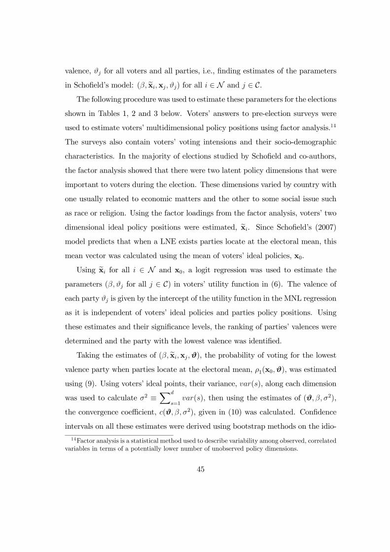
valence, ϑj for all voters and all parties, i.e., finding estimates of the parameters

in Schofield’s model: (β, xi,xj, ϑj) for all i ∈ N and j ∈ C.

The following procedure was used to estimate these parameters for the elections

shown in Tables 1, 2 and 3 below. Voters’answers to pre-election surveys were

used to estimate voters’multidimensional policy positions using factor analysis.14

The surveys also contain voters’voting intensions and their socio-demographic

characteristics. In the majority of elections studied by Schofield and co-authors,

the factor analysis showed that there were two latent policy dimensions that were

important to voters during the election. These dimensions varied by country with

one usually related to economic matters and the other to some social issue such

as race or religion. Using the factor loadings from the factor analysis, voters’two

dimensional ideal policy positions were estimated, xi. Since Schofield’s (2007)

model predicts that when a LNE exists parties locate at the electoral mean, this

mean vector was calculated using the mean of voters’ideal policies, x0.

Using xi for all i ∈ N and x0, a logit regression was used to estimate the

parameters (β, ϑj for all j ∈ C) in voters’utility function in (6). The valence of

each party ϑj is given by the intercept of the utility function in the MNL regression

as it is independent of voters’ideal policies and parties policy positions. Using

these estimates and their significance levels, the ranking of parties’valences were

determined and the party with the lowest valence was identified.

Taking the estimates of (β, xi,xj,ϑ), the probability of voting for the lowest

valence party when parties locate at the electoral mean, ρ1(x0,ϑ), was estimated

using (9). Using voters’ideal points, their variance, var(s), along each dimension

was used to calculate σ2 ≡∑d

s=1var(s), then using the estimates of (ϑ, β, σ2),

the convergence coeffi cient, c(ϑ, β, σ2), given in (10) was calculated. Confidence

intervals on all these estimates were derived using bootstrap methods on the idio-

14Factor analysis is a statistical method used to describe variability among observed, correlatedvariables in terms of a potentially lower number of unobserved policy dimensions.

45

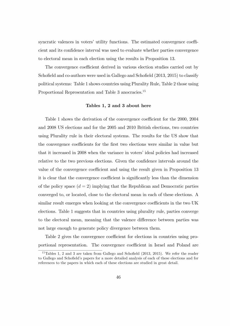
syncratic valences in voters’utility functions. The estimated convergence coeffi -

cient and its confidence interval was used to evaluate whether parties convergence

to electoral mean in each election using the results in Proposition 13.

The convergence coeffi cient derived in various election studies carried out by

Schofield and co-authors were used in Gallego and Schofield (2013, 2015) to classify

political systems: Table 1 shows countries using Plurality Rule, Table 2 those using

Proportional Representation and Table 3 anocracies.15

Tables 1, 2 and 3 about here

Table 1 shows the derivation of the convergence coeffi cient for the 2000, 2004

and 2008 US elections and for the 2005 and 2010 British elections, two countries

using Plurality rule in their electoral systems. The results for the US show that

the convergence coeffi cients for the first two elections were similar in value but

that it increased in 2008 when the variance in voters’ideal policies had increased

relative to the two previous elections. Given the confidence intervals around the

value of the convergence coeffi cient and using the result given in Proposition 13

it is clear that the convergence coeffi cient is significantly less than the dimension

of the policy space (d = 2) implying that the Republican and Democratic parties

converged to, or located, close to the electoral mean in each of these elections. A

similar result emerges when looking at the convergence coeffi cients in the two UK

elections. Table 1 suggests that in countries using plurality rule, parties converge

to the electoral mean, meaning that the valence difference between parties was

not large enough to generate policy divergence between them.

Table 2 gives the convergence coeffi cient for elections in countries using pro-

portional representation. The convergence coeffi cient in Israel and Poland are

15Tables 1, 2 and 3 are taken from Gallego and Schofield (2013, 2015). We refer the readerto Gallego and Schofield’s papers for a more detailed analysis of each of these elections and forreferences to the papers in which each of these elections are studied in great detail.

46

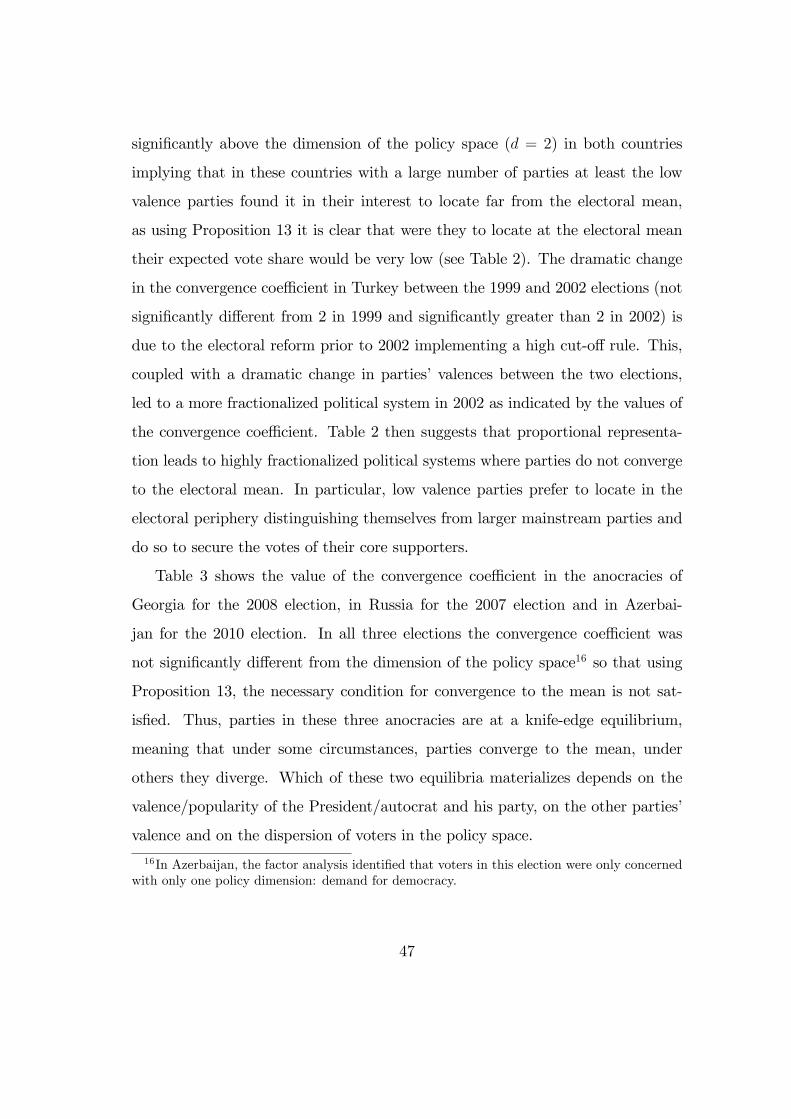
significantly above the dimension of the policy space (d = 2) in both countries

implying that in these countries with a large number of parties at least the low

valence parties found it in their interest to locate far from the electoral mean,

as using Proposition 13 it is clear that were they to locate at the electoral mean

their expected vote share would be very low (see Table 2). The dramatic change

in the convergence coeffi cient in Turkey between the 1999 and 2002 elections (not

significantly different from 2 in 1999 and significantly greater than 2 in 2002) is

due to the electoral reform prior to 2002 implementing a high cut-off rule. This,

coupled with a dramatic change in parties’valences between the two elections,

led to a more fractionalized political system in 2002 as indicated by the values of

the convergence coeffi cient. Table 2 then suggests that proportional representa-

tion leads to highly fractionalized political systems where parties do not converge

to the electoral mean. In particular, low valence parties prefer to locate in the

electoral periphery distinguishing themselves from larger mainstream parties and

do so to secure the votes of their core supporters.

Table 3 shows the value of the convergence coeffi cient in the anocracies of

Georgia for the 2008 election, in Russia for the 2007 election and in Azerbai-

jan for the 2010 election. In all three elections the convergence coeffi cient was

not significantly different from the dimension of the policy space16 so that using

Proposition 13, the necessary condition for convergence to the mean is not sat-

isfied. Thus, parties in these three anocracies are at a knife-edge equilibrium,

meaning that under some circumstances, parties converge to the mean, under

others they diverge. Which of these two equilibria materializes depends on the

valence/popularity of the President/autocrat and his party, on the other parties’

valence and on the dispersion of voters in the policy space.

16In Azerbaijan, the factor analysis identified that voters in this election were only concernedwith only one policy dimension: demand for democracy.

47

The general conclusion from Tables 1, 2 and 3, is that the convergence coef-

ficient varies across elections, countries and political systems and can be used to

classify political systems. In addition, in more fractionalized polities, the valence

of the parties, in particular that of small parties, the weight voters give to the

policy dimensions and the dispersion of voters across the policy space are crucial

elements in determining whether there is convergence to the electoral mean.

Extensions of Schofield’s (2007) model have also been taken to the data to

study the effect that regional parties have in the regional and national elections.

In these models, the voters’utilities depend on the region in which they live and

on the parties competing in that region. Gallego et al (2014) develop and test

a model of the Canadian 2004 federal election in which the Bloc Quebecois runs

only in Quebec. The model studies the effect that the Bloc’s policy positions and

valence had on the electoral outcome in Quebec and how the anticipated outcome

in Quebec and the parties’valences in Quebec and in the rest of Canada affected

the policy positions all parties in both Quebec and the rest of Canada. Labzina

and Schofield (2015) examine the 2010 British general election where the Scottish

National Party ran only in Scotland and Plaid Cymru only in Wales to study the

effect that these two parties and their valences had on the policy positions of all

parties including the national parties (the Conservatives, Labour and the Liberal

Democrats) who ran in Scotland, Wales and England.

The general conclusion of the empirical applications of Schofield -type valence

models is that valence matters in determining the outcome of the election as

the size of the valence advantages of some candidates together with the impor-

tance voters give to the policy dimensions relative to the valence issues determines

whether there is convergence to the electoral mean in different elections in the same

country, across countries and across political regimes.

48

7 The “unified model”à la Adams-Merrill-Grofman

In their 2005 book, Adams, Merrill and Grofman (AMG hereafter) propose a

“unified model”in which voters care both for multi-dimensional policies and for

the parties enacting them. Their modelling of how voters care for parties, and

how this relates with their preferences for policies, is richer than what has been

developed in the preceding sections. Voters differ in their partisanship, with some

being closer to one party and others to another party. Moreover, the members

of one party have different preferences over the policy issues. AMG also add

a random component to the voters’utility, as in section 4. We start with the

description of their model, including some analytical results that they obtain. We

then move to various empirical applications. Finally, AMG add a valence term to

their approach, as in sections 6.1.1 and 6.1.2. Section 7.3 presents some empirical

applications of their unified model with valence in unidimensional policy spaces.

7.1 Theory

There are J ≥ 2 political parties competing for the votes of n citizens by simulta-

neously proposing them policies in a d ≥ 1 policy space. Voter i’s most-preferred

location is denoted by the vector xi, with generic element k denoted by xik. Sim-

ilarly, party j proposes a vector xj with generic element xjk.

The utility of a voter i for party j proposing xj is given by

ui(xj, j) = −∑d

k=1ak(xik − xjk)2 + bjtij + εij. (13)

The first two components of the utility function are assumed to be observable,

while εij is a random variable (from the point of view of parties). The first com-

ponent denotes the utility that voter i derives from policy xj, and is given by the

Euclidean distance between proposed and most-preferred policy. The parameter

49

ak measures the salience of policy dimension k, and is the same for all voters. The

vector tij measures non-policy variables, with coordinate tijl for voter i, party j

and non-policy variable l. For instance, it can measure partisanship, and take a

value of one if voter i identifies with party j, and zero otherwise. The vector bj of

parameters has coordinates bjl, measuring the salience of non-policy issue l when

voting for party j so that the non-policy contribution to voter i’s utility is

bjtij =∑

lbjltijl.

An important aspect of this formulation is that it allows policy preferences to

depend on the vector of non-policy variables tij (for instance, as we will show in

a moment, AMG assume that the distribution of blisspoints xi may differ among

the partisans of different parties).

AMG assumes that the random variables εij are independently generated from

a type I extreme-value distribution. Denote by u∗i (xj, j) the observable component

of voter i’s utility when voting for party j, i.e.,

u∗i (xj, j) = −∑d

k=1ak(xik − xjk)2 + bjtij.

The probability that i votes for j has a logit specification and is given by

ρij(xj, x−j) =exp[u∗i (xj, j)]∑J

j′=1 exp[u∗i (xj′ , j′)].

Party j’s expected vote is the sum of the voting probabilities across voters,17

EVj(xj, x−j) =∑n

i=1ρij(xj, x−j),

17There is no aggregate uncertainty if the number of voters n is suffi ciently large.

50

so that parties maximize their expected vote share EVj.

AMG provides theoretical results when d = 1, in which case

ui(xj, j) = −a(xi − xj)2 + btij + εij,

where tij is a binary party identification variable.

They assume that a proportion mj of voters identifies with party j. Among

those voters, the distribution of blisspoints xi is represented by a density function

fj with mean µj. A fraction m0 of voters are “independent”, meaning that they

do not identify with any party. The overall mean of the blisspoints distribution is

µV , and AMG assume that the average blisspoint of the independents equals µV

(they check empirically that is is the case when they put the model to the data).

AMG (2005, appendix 4.1) have an existence (and uniqueness) theorem, pro-

vided that a condition on endogenous variables is satisfied. Their theorem does

not specify what the equilibrium policies are in equilibrium. Rather, they provide

an algorithm to compute the equilibrium policies numerically. We now list the

main characteristics of these equilibrium policies, starting with the simplest cases.

When b = 0, we are back to the stochastic partisan approach (section 4) with a

unique equilibrium in pure strategies where all parties propose the centrist policy

µV when a is close to zero. If a is larger than zero, then this equilibrium may

not be unique. It is worth emphasizing that this result holds for J ≥ 2– i.e.,

with more than two parties! If J = 2, we obtain a unique equilibrium with policy

convergence to µV even if b > 0 (provided that a is close to zero). This in some

sense generalizes the results obtained for the “probabilistic”approach.

More generally, if J ≥ 3, b > 0 and a tends towards zero, then parties propose

policies which are located in between the centrist position (µV ) and the average

position of their partisans (µk). The reason why vote-seeking candidates shift away

51

from the center in the direction of their partisans is that the marginal change in a

candidate’s probability of attracting her own partisans’votes via policy appeals is

higher than the marginal change in her probability of attracting a rival candidate’s

partisans.

AMG also provide comparative statics analysis of their model. They first

obtain that increasing a (the salience of policy issue) and σ2V (the dispersion of

policy preferences) both lead to more dispersed policies. They obtain the same

qualitative impact when partisans of party j become more extreme (as measured

by average preferred policy µj) and when they become more numerous (larger µj).

This is important, because more extreme parties often have fewer partisans, so

that the two effects go in opposite directions. As we will see with the empirical

applications to France and Norway, this leads to predictions that extreme parties

(such as the communists and the Front National in France, or the Progress party

in Norway) should have, in equilibrium, less extreme policy positions than more

moderate parties! The impact of increasing b (the salience of partisanship) is am-

biguous, but for empirically reasonable values of the parameters a larger value of

b should lead to more extreme parties. Also, increasing the number of parties, J ,

should make policy proposals more extreme for existing parties. Finally, increas-

ing the fraction of independent voters (m0) should lead to more centrist policy

proposals (as, at the limit, if all voters are independent, all parties converge to

the centrist policy µV ).

The AMG (2005) model is similar to Schofield’s (2007), as both predict con-

vergence to the electoral centre. For uniqueness of the equilibrium, AMG require

that the weighted sum of voters’ ideals be contained within an open ball. In

Schofield’s model the convergence condition differs, since the requirement is that

the convergence coeffi cient be less that the dimension of the policy space, d. Like

in the AGM model, convergence in Schofield’s model depends on the variance

52

of voters’ideals along all dimensions but in addition depends on the importance

voters give to the policy dimensions, β, and on the probability that voters chose

the lowest valence party, ρ1(z0,ϑ) in (9) which in turn depends on the valence

differences between the top and lowest valence candidates. It is the interaction of

these three factors through the convergence coeffi cient that determines whether

there is convergence to the mean in Schofield’s (2007) model. If the distribution

of voters’ideals is too dispersed along any dimension, i.e., high σ2, or if the prob-

ability that voters chose the lowest valence party, party 1 is high, a high ρ1(z0,ϑ),

or if voters care a lot about policies, high β, then there is no convergence to the

electoral mean.

We now turn to two applications of this unified model to party positioning in

elections hold in 1988 in France and in 1989 in Norway.

7.2 Applications of the unified model

7.2.1 France 1988 presidential elections

AMG (2005) study the 1988 presidential elections in France. They concentrate

on the five most prominent candidates (representing the extreme left, left, center

right, right and extreme right parties on the left-right dimension) and on the first

round of the election.

They use the answers to Pierce’s 1988 Presidential Election Study by the 748

respondents who have voted in the first round of the election. These respondents

position themselves and the 5 candidates on four different scales numbered from

1 to 7 (so that d = 4): (1) the classical “left-right”one, (2) an immigration scale,

(3) a public sector size scale and (4) a church school scale. They compute the

average position of the 5 candidates on the 4 scales and obtain the same ordering

on all 4 scales.

53

They first test what they call the “policy only model”which corresponds to

utility (13) with bj = 0, so they individuals care about policy only, with some

noise added to make voting probabilistic according to a conditional logit formula.

This model performs poorly when confronted to the data, for two reasons: (1) it

does a bad job at explaining the share of votes obtained by the 5 candidates in

the sample of 748 voters, when the policy positions of the candidates are given

by their average position as determined by these 748 voters and (2) it also does

a very poor job at explaining the policy positions of the five candidates. More

precisely, AMG obtain two types of equilibria, one with full convergence (where

all candidates propose the centrist position in the sample) and one with partial

convergence (where candidates form two blocks, a two-party block proposing a

moderate left policy and a three-party block proposing a moderate right policy).

They conclude that their “policy-only”model, together with the assumption

of vote maximization (which is very close to the stochastic partisanship model

developed in section 4) does a poor job at explaining this election.

AMG then move to the unified model, where they add non-policy preferences

by voters. More precisely, they add as covariates the class, income and gender

of the respondent, and his partisanship (defined as the candidate with whom the

respondent identifies). This model performs much better than the preceding one

on two counts: (1) it explains much better the share of votes that each candidates

received, when candidates policy positions are set at their average location as seen

by the respondents, and (2) it generates nicely dispersed equilibrium positions, in

the four dimensions studied (left-right, immigration, public sector size and atti-

tude toward church schools). AMG report results on the left-right scale, where

the expected vote functions are nicely concave in a candidate position when all

other candidates positions are kept fixed (at their computed equilibrium value).

The equilibrium positions are less extreme than the mean position advocated by

54

the partisans of the party, which is in line with the theoretical results provided

above. At the same time, two characteristics of the equilibrium are not found in

the actual candidates positions. First, the extreme parties (the communists and

the Front National) adopt at equilibrium less extreme policies than the moder-

ate (socialists and RPR, respectively) parties. This result falls in line with the

theoretical results presented above, but clashes with the real position of these par-

ties. AMG suggest that extreme political parties do not maximize their expected

vote, but rather an objective which induces them to be more extreme than if they

maximized expected vote. Second, the equilibrium policies are less extreme than

those observed in reality. One way to make the equilibrium policies more extreme

is to introduce the “unified model with discounting”where voters consider that

parties will not be able to enact their announced policy when elected, but rather

will cover the fraction 1 − dj of the distance between a status quo position SQ

and the announced policy xj, so that the policy preference of voter i becomes

−a(xi − (SQ+ (1− dj)(xj − SQ)))2.

Not surprisingly, this modified model (1) generates less convergent (i.e., more

extreme) policy proposals by parties and (2) better fits the empirical data (since

there is an additional degree of freedom in the estimation of the parameter dj).

The estimated value of the parameter (assumed to be the same for all parties j)

is dj = 0.34, meaning that voters discount candidates’promises by one third (and

believe that a candidate will, if elected, move the actual policy to two-thirds of

the distance between the status quo (exogenously set at the mid—point of the 1-7

scale) and the policy advertised by the candidate.

55

7.2.2 Norway 1989 elections

AMG proceed in a similar way to study the 1989 elections in Norway, which

counts 7 different parties. They obtain very similar results, with the “policy-

only”model incapable of reproducing the vote shares and policy positions of the

parties, and the “unified model” performing much better on both counts, but

generating positions which are (1) less extreme than the actual positions observed

and (2) such that the extreme right (Progress) party proposes a more centrist

position than the right party. The introduction of discounting in this unified

model also allows to generate more extreme policies, moving them closer to the

observed positions (with a discounting factor dj = 0.47).

AMG also consider an extension to their model, which includes the fact that

parties form one of two coalitions in Norway: a left-wing coalition comprised of two

parties, or a right wing (comprised of 3 parties) (the Liberal and Progress parties

were not potential members of either traditional bloc in 1989). They then consider

that a party maximizes a weighted sum of its expected vote share and of the vote

share of its coalition partners, with a relative weight of α on the latter. They

obtain numerically a unique Nash equilibrium for exogenous values of α (set at

0.5 and 0.75), while a Nash equilibrium does not exist for α = 1. The equilibrium

policies are actually not very responsive to the value of α, showing that moving

to coalition considerations does not affect much the parties’equilibrium policies.

Out of 7 parties, 4 equilibrium policies move closer to the actual policy positions,

including the extreme-right party whose position becomes more extreme.

7.3 Adding valence to the empirical unified model

In the two empirical applications with 2 candidates (J = 2) (France’s second round

and US presidential elections, both held in 1988), AMG add a valence component

56

(modelled as in section 6.1) to their unified model. They first estimate a con-

ditional logit voting model with partisanship (and other covariates), where they

interpret the intercept of the conditional logit equation for the winning candidate

(Mitterrand for France, Bush for the US) as the valence of this candidate.18

Before introducing uncertainty (as to the candidate’s valence or the election

results), they use this model to answer several questions. First, could the losing

candidate have won the elections by choosing another policy (keeping the policy of

the winner constant)? The answer is negative, showing that the winner’s valence

advantage was large enough to prevent the valence disadvantaged candidate from

winning. Second, they measure the policy leeway of the winner by computing the

range of policies he could have proposed while still winning the election, whatever

the policy choice of his opponent. They find quite large policy intervals for both

countries, which they call the “dominance zone”of the election winner. This in

turn means that the eventual winner had quite a lot of leeway to move close to

his most-preferred policy, while the valence disadvantaged candidate had no such

leeway and had to remain closer to the mean of the electorate.

They then introduce uncertainty for the valence of the winning candidate, as-

suming that this parameter (given by the intercept of their regression) is normally

distributed with some standard deviation σV . This model being much more com-

plex than the simple one developed in section 6.1.2, they can not focus on the

median voter’s voting behavior. Rather, they make the assumption (which they

call approximation) that the valence uncertainty generates a normal distribution

of the expected vote share of both candidates, with a standard deviation which

18AMG also study the 1997 UK election. They exogenously fix the Liberal Democrat party’spolicy at its observed position, and they endogenize the policy positions of the other two parties(Labour and Conservative). The rationale for this approach is that pre-election polls gave theLib-Dem no chance at all of winning the general election, and that the implemented policyis assumed to be the one proposed by the party obtaining the plurality. They obtain resultsqualitatively very similar to those reported here for the France and US 1988 elections.

57

does not vary with the candidates positions. In other words, the expected vote

share of candidate j is given by EVj(xj, x−j) + ε, where EVj(xj, x−j) is computed

from the unified model estimated above, and where ε is normally distributed with

a standard deviation of σε. The probability of winning of party j is then given by

πi(xj, x−j) = Φ

(EVj(xj, x−j)− 0.5

σε

),

where Φ denotes the cdf of the normal distribution.

Solving the model numerically for both of France and the US, they obtain an

equilibrium in pure strategies.19 They obtain in both cases that (1) the valence

advantaged candidate proposes at equilibrium a policy close to his most-preferred

policy (exogenously set for this exercise) while the valence disadvantaged candi-

date locates much closer to the average position of the electorate, and (2) that

both candidates propose more extreme policies than the ones they would have

proposed if their objective had been to maximize their probability of winning the

elections. These two results give strong support to the theoretical predictions

made at the end of section 6.1.2. Moreover, they obtain that the dispersion be-

tween equilibrium policy proposals increases with σε. Intutively, as the perceived

election probability becomes less responsive to shift in policies (because of more

valence uncertainty generating more uncertainty as to the winning probabilities),

parties obtain more leeway to move closer to their most-preferred policies xj.

AMG also apply the model of electoral uncertainty developed in section 6.1.1,

to the 1988 elections in France and in the US, and the 1997 elections in the UK.

They assume that the uncertainty in the location of the median voter translates

into an uncertain distribution of the expected vote shares of the parties, with a19They depict the expected utility and expected probability of winning of both candidates, as

a function of the candidate’s policy proposal, when his opponent policy proposal is fixed at hisequilibrium values. The curves depicted are not everywhere quasi-concave, but they do exhibita global maximum.

58

standard deviation increasing with the distance between the parties’policy pro-

posals. So, the assumption that the median location is set atm+ε with ε normally

distributed around zero with standard deviation σm translates into an expected

vote function normally distributed with a standard deviation σu defined by

σu = sσm |xA − xB| ,

with s a parameter whose value is inferred from the data. They then proceed to

numerical simulations of the two parties’equilibrium locations as a function of

their (exogenously set) ideologically preferred most-preferred points and amount

of uncertainty σm. They obtain a substantial amount of policy dispersion be-

tween the two parties even with low values of σm. For such low values, the

valence-advantaged candidate is more extreme than the other candidate, while

the opposite occurs for large values of σm. They then argue that the former case

corresponds better to developed countries where the pre-election polls are usually

quite informative, while the latter case (the “extreme underdog” effect) would

rather occur in less developed countries where pre-election polls are less infor-

mative. To the best of our knowledge, this conjecture concerning less developed

countries has not yet been put to the data.

8 Conclusion

This paper has surveyed the literature dealing with the positioning of political

parties in uni- and multi-dimensional policy spaces. Constraints on the length of

the paper have prevented us from surveying all contributions to this rich literature.

A notable limitation of our survey is the restriction to models with an exogenous

number of parties who commit to implement their policy proposals once elected.

We have tried to focus on the main contributions, as well as on the more recent

59

ones. Our main focus is on theoretical contributions, but we also survey papers

providing empirical applications of the theoretical concepts developed.

We first show that, in the absence of uncertainty, parties converge to the same

policy whether they are electorally or policy motivated when the policy space is

unidimensional, and that there is generically no equilibrium in pure strategies

for multidimensional policy spaces. The first conclusion we draw is then that

introducing some form of uncertainty as to the election results is primordial.

We first survey the papers assuming that voters’preferences are affected by

a random shock determining the bias the voter has for one of the two parties,

the so-called stochastic partisanship approach. The main result is that parties

converge to the same policy when a Nash equilibrium in pure strategies exists,

but that equilibrium existence requires a suffi ciently large amount of uncertainty.

It is worth stressing this point, often forgotten by contributions making use of

this approach, since it indicates that stochastic partisanship probabilistic voting

can actually create existence problems even in one-dimensional settings where a

deterministic, Downsian equilibrium in pure strategies exists.

We then move to an alternative way of introducing uncertainty assuming that

voters do not have partisan preferences, but rather that parties are uncertain as

to the policy preferences of voters. There are important equilibrium existence

issues when parties have electoral motivations, so that we concentrate on policy

motivations. Although there is no satisfactory general existence theorem, the

so-called Wittman equilibrium often exists in uni-dimensional policy spaces, and

exhibits the nice property (empirically validated) that parties do not converge

to the same policy. Unfortunately, equilibria generically fail to exist in multi-

dimensional policy spaces. We then examine the approach pioneered by Roemer,

where parties are composed of two factions, one having electoral motivations while

the other has policy objectives. The resulting Party Unanimity Nash Equilibria

60

often exist, and several papers provide empirical applications of this approach.

Next, we survey models in which candidates’electoral prospects depend on a

valence component– voters’non-policy evaluation of candidates– and where all

voters agree that one party has better characteristics than another. In a one-

dimensional policy model with valence and no unceratinty with two win and offi ce

motivated candidates, Groseclose (2001) proves the non-existence of Nash equilib-

ria in pure strategies. The intuition behind this result is that at any position one of

the two candidates wants to move. This result extends to multidimesinonal policy

two candidates models with no uncertainty, thus showing the knife-edge quality

of the Downs and Wittman results in valence models. Extensions of Gloseclose’s

model with mixed strategy Nash equilibria are discussed in the Appendix showing

that the knife-edge property of the Downsian model is an illusion since the mixed

strategy Nash equilibrium converges to the Downsian pure strategy equilibrium

when the valance advantage converges to zero. In a two-candidate one-dimensional

model with valence, Londregan and Romer (1993) show the existence divergent

policy platforms when parties are uncertain as to candidates’ability to generate

constituency services in which the degree of policy polarization increases in the

importance voters’give to the valence issue.

We then examine multi-dimensional policy models in which voters rank can-

didates along a single valence dimension. These models derive the necessary and

suffi cient conditions for the existence of a Nash equlibrium. Ansolabehere and

Snyder (2000) show that equilibrium existence in a win-motivated two-candidate

no uncertainty model depends on voters’ ideal policies not being too dispersed

in the policy space, but that equilibria typically fail to exist when candidates

maximize their vote share rather than their probability of wining.

Schofield’s (2007) multi-dimensional multi-candidate model shows that can-

didates converge to the electoral mean if the convergence coeffi cient is less that

61

the dimension of the policy space and this happens when voters do not give too

much importance to the policy space (or alternatively, when votes give greater

importance to the valence issue), when their ideal policies are not too dispersed

and when the probability of voting for the lowest valence candidate —when all can-

didates locate at the electoral mean—is high enough so that the valence difference

between the the lowest valence and all other candidates is not too large. We then

examine extensions to Schofield’s (2007) model to elections with regional parties

tha affect convergence to the electoral mean.

We also study Schofield’s (2006) endogenous valence model where activists

contribute resouces of time and money in an effort to influence candidates’policy

positions when candidates use these resources to influence voters’decisions. This

endogenous valence model shows that in equilibrium candidates’locate where the

activist and electoral pulls balance each other. The section ends with a discussion

of the empirical evidence on valence models as applied to several elections in

various countries under various political regimes.

In the final section, we present the “unified model” developed by Adams,

Merrill and Grofman where voters care both for multi-dimensional policies and for

the parties enacting them. More precisely, voters differ in their partisanship, with

some being closer to one party and others to another party, with this partisanship

affecting their policy preferences. This unified model has been fruitfully applied

to several elections, such as the 1988 French presidential elections, and the 1989

election in Norway. We also consider an empirical extension where valence is added

to this unified model.

62

9 Appendix: Equilibria in mixed strategy with

valence and offi ce motivation

Aragones and Palfrey (2002) solve the mixed strategy equilibrium version of the

Groseclose model where candidates chose from a finite number of position and

candidate A has an infinitesimal valence advantage (e.g., value of holding offi ce,

incumbent performance, constituency service, campaign advertising) over candi-

date D. Candidates maximize their probability of winning but don’t know the

location of the median voter’s ideal point. They assume that voters vote for A

unless D is closer to the voter’s ideal by some fixed distance, δ. In general, there

is no pure strategy Nash equilibria. In their unique symmetric mixed strategy

equilibrium with no gaps, candidates randomize over a fairly small number of po-

sitions in a region near the expected median. They show that as the number of

positions becomes fairly large– so that the policy space approximates a continu-

ous space– the region over which candidates chose positions converges to that of

the expected median voter’s position. They find that as A’s advantage converges

to zero, the equilibrium probability of winning converges to 1/2. This continuity

result also depends on the valence dimensions playing a minor role in the election.

Aragones and Palfrey conclude the knife-edged property of the Downsian model is

an illusion since the distribution of strategies in the mixed equilibrium converges

to the Downsian pure strategy equilibrium.

In their 2005 paper, Aragones and Palfrey argue that the limitations of their

2002 model is that (1) candidates do not have preferences over policies; (2) hard to

imagine how candidates implement mixed strategies; and (3) candidates have per-

fect information about the objective function of her opponent. Aragones and Pal-

frey (2005) argue that by adding private information they can justify mixed strat-

egy equilibrium and relax these assumptions in a two-candidate two-dimensional

63

asymmetric information model where one candidate has a quality advantage and

candidates care about policies and winning. The weight placed on winning and

their ideal policy are the candidate’s private information with the weight drawn

independently of each candidate from a commonly known distribution. The me-

dian voter’s ideal point is drawn from a distribution common to both candidates.

They show that candidates locate at the center if and only if her value of holding

offi ce is suffi ciently high. They also show that the advantaged (disadvantaged)

candidate A (D) is more (less) likely to locate at the centre the more likely D

(A) is to locate at the centre. An increase in the uncertainty about the median

voter’s ideal point (or alternatively, as the electorate becomes more polarized)

makes both candidates more likely to adopt more polarized policies. They show

that the equilibrium policies converge to those of Aragones and Palfrey (2002) as

the weight candidates give to policies converges to zero.

Aragones and Xefteris (2012) develop a two-candidate Downsian model in

which one candidate has a valence advantage and the policy space is continuous.

They assume that voters have quadratic (rather than Euclidean) policy prefer-

ences, thus making candidates payoff functions continuous (rather than discon-

tinuous) so that the best response function of the disadvantaged candidate is well

(rather than not well) defined. They study the pure strategy Nash equilibria when

candidates’beliefs on the distribution of the median’s ideal policy is unimodal. In

equilibrium, the advantaged candidate chooses to locate at the expected median

voter’s ideal with probability one and the disadvantaged candidate chooses to lo-

cate with equal probability at one of two policies symmetrically located about the

expected median. Their results show that an equilibrium exists for any size (small

enough so that there is no pure strategy equilibria) of the advantage if and only

if the variance of the location of the median voter’s ideal is low enough relative

to the size of the advantage, i.e., when candidates believe that the median voter’s

64

ideal is close enough to 1/2 with high enough probability. The advantage can-

didate adopts policies that are more moderate than the disadvantaged one with

the advantage candidate having a larger probability of winning than the disad-

vantaged candidate. Moreover, they find that as the advantage increases so does

the probability of the advantaged candidate winning, candidates’policies become

more differentiated, and the existence conditions on the variance of the median’s

ideal are relaxed. As the advantage disappears, the disadvantaged candidate’s pol-

icy moves closer to the advantage one, thus converging to the standard Downsian

model where both candidates converge to the expected median.

65

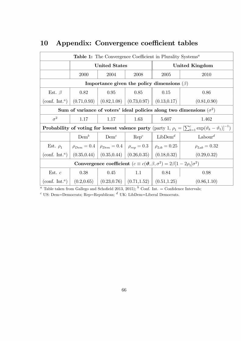
10 Appendix: Convergence coeffi cient tables

Table 1: The Convergence Coeffi cient in Plurality Systemsa

United States United Kingdom

2000 2004 2008 2005 2010

Importance given the policy dimensions (β)

Est. β 0.82 0.95 0.85 0.15 0.86

(conf. Int.a) (0.71,0.93) (0.82,1.08) (0.73,0.97) (0.13,0.17) (0.81,0.90)

Sum of variance of voters’ideal policies along two dimensions (σ2)

σ2 1.17 1.17 1.63 5.607 1.462

Probability of voting for lowest valence party (party 1, ρ1 = [∑c

k=1 exp(ϑk − ϑ1)]−1)

Demb Demc Repc LibDemd Labourd

Est. ρ1 ρDem = 0.4 ρDem = 0.4 ρrep = 0.3 ρLib = 0.25 ρLab = 0.32

(conf. Int.a) (0.35,0.44) (0.35,0.44) (0.26,0.35) (0.18,0.32) (0.29,0.32)

Convergence coeffi cient (c ≡ c(ϑ, β, σ2) = 2β[1− 2ρ1]σ2)

Est. c 0.38 0.45 1.1 0.84 0.98

(conf. Int.a) (0.2,0.65) (0.23,0.76) (0.71,1.52) (0.51,1.25) (0.86,1.10)a Table taken from Gallego and Schofield 2013, 2015); b Conf. Int. = Confidence Intervals;c US: Dem=Democrats; Rep=Republican; d UK: LibDem=Liberal Democrats.

66

Table 2: The Convergence Coeffi cient in Proportional Systemsa

Israel Turkey Poland1996 1999 2002 1997Weight of policy differences (β)

Central Est.b of β 1.207 0.375 1.520 1.739(conf. Int.c) (1.076,1.338) (0.203,0.547) (1.285,1.755) (1.512,1.966)

Electoral variance (trace5 = σ2)σ2 1.732 2.34 2.33 2.00

Probability of voting for lowest valence party (party 1, ρ1 = [∑p

k=1 exp(ϑk − ϑ1)]−1)

TWd FPe ANAPe ROPf

Central Est.b of ρ1 ρITW = 0.014 ρFP = 0.08 ρTANAP = 0.08 ρPROP = 0.007(conf. Int.c) (0.006,0.034) (0.046,0.145) (0.038,0.133) (0.002,0.022)

Convergence coeffi cient (c ≡ c(ϑ, β, σ2) = 2β[1− 2ρ1]σ2)Central Est.b of c 4.06 1.49 5.75 5.99(conf. Int.c) (3.474,4.579) (0.675,2.234) (4.388,7.438) (5.782,7.833)

a Table taken from Gallego and Schofield 2013, 2015); b Central Est. = Central Estimate;c Conf. Int. = Confidence Intervals; d Israel: TW = Third Way;e Turkey: DYP =True Path Party. f Poland: ROP = Movement for Reconstruction of Poland.

Table 3: The Convergence Coeffi cient in Anocraciesa

Georgia Russia Azerbaijane

2008 2007 2010Weight of policy differences (β)

Est. β 0.78 0.181 1.34(conf. Int.b) (0.66, 0.89) (0.15,0.20) (0.77,1.91)

Electoral variance (trace5 = σ2)σ2 1.73 5.90 0.93

Probability of voting for lowest valence party (party 1, ρ1 = [∑p

k=1 exp(ϑk − ϑ1)]−1)

Nd SRc AXCP-MPd

Est. ρ1 ρGN = 0.05 ρRSR = 0.07 ρAXCP−MP = 0.21(conf. Int.a) (0.03,0.07) (0.04,0.12) (0.08,0.47)

Convergence coeffi cient (c ≡ c(ϑ, β, σ2) = 2β[1− 2ρ1]σ2)Est. c 2.42 1.83 1.44

(conf. Int.a) (1.99,2.89) (1.35,2.28) (0.085,2.984)a Table taken from Gallego and Schofield 2013, 2015); b Conf. Int. = Confidence Intervals;c Georgia:.N=Natelashvili; d Russia: SR=Fair Russia;eAzerbaijan: AXCP-MP=Azerbaijan Popular Front Party (AXCP) and Musavat (MP).

The estimates for Azerbaijan are less precise because the sample is small.

67

References

[1] Adams JF, Merrill S, Grofman B. 2005. A unified theory of party competition:a cross-national analysis integrating spatial and behavioral factors.CambridgeUniversity Press.

[2] Ansolabehere S, Snyder JM. 2000. Valence Politics and Equilibrium in SpatialElection Models. Public Choice, 103(3):327-336.

[3] Ansolabehere S, Snyder JM, Stewart C. 2001. Candidate Positioning in U.S.House Elections. American Journal of Political Science 45(1):136—159.

[4] Aragones E, Palfrey T. 2002. Mixed Equilibrium in a Downsian Model witha Favored Candidate. Journal of Economic Theory, 103(1):131—161.

[5] Aragones E, Palfrey T. 2005. Electoral Competition Between Two Candi-dates of Different Quality: The Effects of Candidate Ideology and PrivateInformation. In Social Choice and Strategic Decisions: Essays in Honor ofJeffrey S. Banks eds D Austen-Smith, J Duggan. Springer.

[6] Aragones E, Xefteris D. 2012. Candidate quality in a Downsian model witha continuous policy space. Games and Economic Behavior, 75(2):464—480.

[7] Austen-Smith D, Banks J. 1999. Positive Political Theory I: Collective Pref-erences. Ann Arbor, MI: University of Michigan Press.

[8] Banks J. 1995. Singularity Theory and Core Existence in the Spatial Model,Journal of Mathematical Economics, 24:523—536.

[9] Banks J, Duggan J. 2005. Probabilistic Voting in the Spatial Model of Elec-tions: The Theory of Offi ce-motivated Candidates. in Social Choice andStrategic Decisions: Esssays in honour of J. Banks, Part of the series Studiesin Choice and Welfare, pp 15-56.

[10] Banks J, Duggan J, Le Breton M. 2002. Bounds for Mixed Strategy Equilibriaand the Spatial Model of Elections, Journal of Economic Theory, 103:88—105.

[11] Calvert R, 1985. Robustness of the Multidimensional Voting Model: Candi-date Motivations, Uncertainty, and Convergence. American Journal of Polit-ical Science 29 (1):69—95.

[12] Calvert R, 1986. Models of Imperfect Information in Politics, London: Har-wood Press.

68

[13] Caplin A, Nalebuff B. 1988. On 64% Majority Rule. Econometrica, 56:787—814.

[14] Caplin A, Nalebuff B. 1991. Aggregation and Social Choice: A Mean VoterTheorem. Econometrica, 59:1—23.

[15] Clarke, H, Kornberg A, MacLeod J, Scotto, T. 2005. Too Close to Call:Political Choice in Canada, 2004. PS: Political Science and Politics, 38: 247-253.

[16] Clarke, H, Kornberg A, Scotto, T. 2009. Making Political Choices. Toronto:Toronto University Press.

[17] Clarke, H, Sanders D, Stewart M, Whiteley P. 2005. Political Choice inBritain. Oxford: Oxford University Press.

[18] Clarke, HD, Sanders D, Stewart M, Whiteley P. 2009. Performance Politicsand the British voter. Cambridge: Cambridge University Press.

[19] Clarke, H, Scotto, T, Kornberg A. 2011. Valence Politics and Economic Crisis:Electoral Choice in Canada 2008. Electoral Studies 30(3):438-449.

[20] Cohen L, Mathews S. 1980, Constrained Plott Equilibria, Directional Equi-libria and Global Cycling Sets, Review of Economic Studies, 47:975—986.

[21] Coughlin P, 1992, Probabilistic Voting Theory. Cambridge University Press.

[22] Cox G. 1987. The Uncovered Set and the Core. American Journal of PoliticalScience, 31:408—422.

[23] Cremer H, De Donder Ph, Gahvari F. 2008. Political Competition within andbetween Parties: An Application to Environmental Policy. Journal of PublicEconomics, 92 (3-4):532-547.

[24] De Donder P, Hindriks J. 2007. Equilibrium social insurance with policy-motivated parties. European Journal of Political Economy, 23:624-640.

[25] Downs A. 1957. An Economic Theory of Political Action in a Democracy.Journal of Political Economy 65 (2):135—150.

[26] Duggan J. 2006a. A Note on Uniqueness of Electoral Equilibrium When theMedian Voter is Unobserved. Economics Letters, 92:240—244.

[27] Duggan J. 2006b. Candidate Objectives and Electoral Equilibrium. In: Wein-gast BR , Wittman DA (eds) The Oxford handbook of political economy. Ox-ford University Press, Oxford.

69

[28] Duggan J. 2014. A Survey of Equilibrium Analysis in Spatial Models of Elec-tions, mimeo, University of Rochester.

[29] Duggan J, Fey M. 2005. Electoral Competition with Policy-Motivated Can-didates, Games and Economic Behavior, 51:490-522.

[30] Duggan J, Jackson M. 2005. Mixed Strategy Equilibrium and Deep Coveringin Multidimensional Electoral Competition, mimeo.

[31] Eaton C, Lipsey R. 1975. The Principle of MinimumDifferentiation Reconsid-ered: Some New Developments in the Theory of Spatial Competition, Reviewof Economic Studies, 42:27—49.

[32] Enelow J, Hinich M. 1989. A general probabilistic spatial theory of elections.Public Choice, 61(2):101-113.

[33] Feld SL, Grofman B, Miller N. 1988. Centripetal forces in spatial voting: Onthe size of the Yolk. Public Choice, 59(1):37-50.

[34] Fiorina MP. 1973. Electoral margins, constituency influence, and policy mod-eration: A critical assesment. American Politics Quarterly, 1(4):479-498.

[35] Gallego M, Schofield N. 2013. The convergence coeffi cient across politicalregimes. The Scientific World Journal, Article ID 653035, 28 pages.

[36] Gallego M, Schofield N, McAlister K, Jeon JS. 2014. The variable choiceset logit model applied to the 2004 Canadian election. Public Choice, 158(3-4):427-463.

[37] Gallego M, Schofield N. 2015. Do parties converge to the elec-toral mean in all political systems? Journal of Theoretical Politics,doi:10.1177/0951629815586878.

[38] Gallego M, Schofield N. 2016a. Modelling the effect of campaign advertisingon US presidential elections. forthcoming In The Political Economy of SocialChoices, eds N Schofield, M Gallego. Springer.

[39] Gallego M, Schofield N. 2016b. Modelling the effect of campaign advertisingon US presidential elections when differences across states matter. Unpub-lished manuscript.

[40] Groseclose T. 2001. A Model of Candidate Location When One Candidatehas a Valence Advantage. American Journal of Political Science, 45:862—886.

70

[41] Hinich M. 1977. Equilibrium in Spatial Voting: The Median Voter Result isan Artifact. Journal of Economic Theory, 16:208—219.

[42] Hinich M. 1978. Some evidence on non-voting models in the spatial theoryof electoral competition. Public Choice, 33(2):83-102.

[43] Hinich M, Ledyard J, Ordeshook P. 1972. Nonvoting and the existence ofequilibrium under majority rule. Journal of Economic Theory, 4(2):144—153.

[44] Hinich M, Ledyard J, Ordeshook P. 1973. A Theory of Electoral Equilibrium:A Spatial Analysis Based on the Theory of Games, Journal of Politics, 35:154-193.

[45] Hotelling H. 1929. Stability in competition. Economic Journal. 39:41-57.

[46] Labzina E, Schofield N. 2015. Application of the Variable Choice Logit Modelto the British General Election of 2010. In The Political Economy of Gover-nance:Institutions, Political Performance and Elections, eds N Schofield, G.Caballero. Springer.

[47] Laussel D, Le Breton M. 2002. Unidimensional Downsian politics: median,utilitarian or what else? Economics Letters 76:351—356.

[48] Lee W, Roemer JE. 2006. Racism and redistribution in the United States:A solution to the problem of American exceptionalism. Journal of PublicEconomics. 90(6):1027-1052.

[49] Lindbeck A, Weibull J. 1987. Balanced-budget redistribution as the outcomeof political competition. Public Choice, 52(3):273-297.

[50] Lindbeck A, Weibull J. 1993. A model of political equilibrium in a represen-tative democracy. Journal of Public Economics, 51(2):195-209.

[51] Londregan J, Romer T. 1993. Polarization, Incumbency, and the PersonalVote. In Political Economy: Institutions, Competition and Representationeds WA Barnett, MJ Hinich and N Schofield. Cambridge University Press.

[52] McKelvey R. 1976. Intransitivities in Multidimensional Voting Models andSome Implications for Agenda Control. Journal of Economic Theory, 12:472—482.

[53] McKelvey R. 1979. General Conditions for Global Intransitivities in FormalVoting Models, Econometrica, 47:1085—1111.

71

[54] McKelvey R. 1986. Covering, Dominance and Institution-Free Properties ofSocial Choice, American Journal of Political Science, 30:283—314.

[55] McKelvey R, Schofield N. 1986. Structural Instability of the Core, Journal ofMathematical Economics, 15:179—198.

[56] McKelvey R, Schofield N. 1987. Generalized Symmetry Conditions at a CorePoint, Econometrica, 55:923—933.

[57] Persson T, Tabellini GE. 2000. Political economics: explaining economic pol-icy. The MIT Press.

[58] Plott C. 1967. A Notion of Equilibrium and its Possibility Under MajorityRule. The American Economic Review, 57(4):787—806.

[59] Riker W, Ordeshook P. 1973. An introduction to positive political theory.Prentice Hall.

[60] Roemer JE. 1994. A theory of policy differentiation in single issue electoralpolitics. Social Choice and Welfare, 11:355-380.

[61] Roemer JE. 1997. Political—economic equilibrium when parties represent con-stituents: The unidimensional case. Social Choice and Welfare, 14(4):479-502.

[62] Roemer JE. 1998. Why the poor do not expropriate the rich: an old argumentin new garb. Journal of Public Economics 70(3):399-424.

[63] Roemer JE. 1999. The democratic political economy of progressive incometaxation. Econometrica, 67(1):1-19.

[64] Roemer JE. 2001. Political Competition: Theory and Applications, Cam-bridge: Harvard University Press.

[65] Roemer JE. 2006. Modeling Party Competition in General Elections, OxfordHandbook of Political Economy, eds. B. Weingast, D. Wittman, pp. 1010-1030.

[66] Roemer JE. 2009. Political competition: Theory and applications. HavardUniversity Press.

[67] Saari D. 1997. The Generic Existence of a Core for q-Rules, Economic Theory,9:219—260.

[68] Schofield N. 1978. Instability of Simple Dynamic Games, Review of EconomicStudies, 45:575—594.

72

[69] Schofield N. 1983. Generic Instability of Majority Rule, Review of EconomicStudies, 50:695—705.

[70] Schofield N. 1984. Social Equilibrium and Cycles on Compact Sets. Journalof Economic Theory, 33:59—71.

[71] Schofield N. 1985. Social Choice and Democracy. Berlin: Springer.

[72] Schofield N. 2006. Equilibria in the Spatial Stochastic Model of Voting withParty Activists. The Review of Economic Design, 10(3):183-203.

[73] Schofield N. 2007. The Mean Voter Theorem: Necessary and Suffi cient Con-ditions for Convergent Equilibrium. Review of Economic Studies, 74:965—980.

[74] Stokes, D. 1963. Spatial Models of Party Competition, American PoliticalScience Review 57(2):368-377.

[75] Stokes, D. 1992. Valence Politics. In Electoral politics ed. by D Kavanagh.Claredon Press. Oxoford.

[76] Wittman D, 1977, Candidates with Policy Preferences: A Dynamic Model,Journal of Economic Theory, 14:180-189.

[77] Wittman D, 1983. Candidate Motivation: A Synthesis of Alternative Theo-ries. American Political Science Review, 77(1):142-157.

[78] Wittman D, 1990. Spatial strategies when candidates have policy preferences.In Advances in the Spataial Theory of Voting, eds. JM Enelow, MJ Hinich,Cambridge University Press.

73