2013-31

Dynamic effect of inter-airline rivalry on airfares and consumers’ welfare:

Japan’s full-service vs. new air carriers

Hideki Murakami　Yoshihisa Amano

Dynamic effect of inter-airline rivalry on airfares and consumers’ welfare:

Japan’s full-service vs. new air carriers

Hideki MURAKAMI and Yoshihisa AMANO

Abstract. We analyzed the dynamic changes in carriers’ airfares and outputs and computed the

changes in the consumers’ surplus year by year after new Japanese carriers entered thriving

routes and started to compete with Japanese full-service airlines (FSAs). Using unbalanced

panel data of 222 route-and-carrier-specific sample observations, we found that new carriers

discounted airfares significantly as soon as they entered new markets, but two early-comers,

Skymark Airlines and AIRDO that had entered with very low airfares raised their price year by

year. The two FSAs All Nippon Airways and Japan Airlines responded to the new entrants and

lowered their airfares to a much lesser extent than new entrants did, and kept their airfare levels

almost unchanged for at least four years from the first entry, although a tiny fluctuation of

airfares was recognized. The consumers’ surplus increased significantly in the first year of new

entries but gradually reduced as new entrants raised their airfares.

Key words: Japanese airlines, entry, dynamic change in airfare, consumers’ surplus

1. Introduction

In 1996, the Ministry of Transport of Japan authorized Skymark Airlines (SKY) and AIRDO

(ADO) to commence operations. These new entries were followed by Skynet Asia Airways

(SNA, now renamed Solaseed Air) and Star Flyer Inc. (SFJ), founded in 2000 when the

Japanese Ministry of Land, Infrastructure, and Transport deregulated airlines’ entry and exit and

airfares.

These new airlines were initially referred to as low-cost carriers (LCCs). However,

although new Japanese carriers have some features of LCCs in common with those of other

countries in terms of route-by-route service and low airfares, the services and cost structures of

Japan’s new entrants differ from those of foreign LCCs. The most salient difference between the

foreign LCCs and new Japanese carriers is that, unlike the situation in the U.S., Japan’s

metropolitan areas do not have secondary commercial airports available for LCCs. In addition,

the cost structures of the new Japanese carriers are almost the same as those of full-service

airlines (FSAs) except for the new carriers’ low labor cost. The airplane-maintenance cost of the

new carriers could be more expensive than those of the FSAs, however. The reason is that new

carriers do not have their own maintenance subsidiary company or division, and they had to

arrange to have the maintenance performed by the FSAs. Since FSAs charge the new carriers

high maintenance fees in order to weaken the new carriers’ cost competitiveness, the new

carrie

maint

witho

amon

FSAs

the co

The a

and J

finan

Sourc

JAL:

Skym

airlin

The a

mark

motiv

and h

estim

dumm

airfar

ers are com

tenance cost

out simplifyi

ng Japanese

s. However,

osts of the ne

Figure 1 de

average costs

JAS). In fact

ncial support

Fig.

ce: JAA Civil A

Japan Airlines

mark Airlines;

We analyze

nes (i.e., SKY

analysis inclu

ket in which s

Having obs

vated to anal

how the ma

mated the str

my variables

res and passe

In Section

mpelled to l

s. In addition

ng the servic

airlines; thu

the Japanese

ew Japanese

epicts the ave

s of the new

t, ADO wen

from the Ind

1. Changes

Aviation Data

s; ANA: All N

SNA: Solasee

ed the dynam

Y, ADO, SNA

uded not onl

several new a

served the air

lyze the mark

arket perform

ructural dem

s for the new

enger volume

2, we revie

ower their

n, new Japan

ce, and costs

us, there is n

e governmen

new airlines

erage cost of

carriers did

nt bankrupt i

dustrial Revit

in Japanese

abook and fina

Nippon Airway

ed Air; SFJ, St

mic price com

A, and SFJ).

ly the duopo

airlines have

rline regulato

ket performa

mance has c

mand and qu

w entrants an

e after the ne

ew the litera

input price

nese airlines

such as land

not much dif

nt imposes a

s are higher t

f seven Japan

not differ gr

in 2002, and

talizing Corp

airlines’ ave

ancial stateme

ys; JAS: Japan

tar Flyer Inc.

mpetition bet

. The carrier

oly market (i

e entered.

ory reforms

ance for the r

changed over

uasi-supply

nd for the FS

ew carriers en

ature on the

s such as l

offer some f

ding fees, fue

fference betw

a tax for the

than those of

nese airlines

reatly from th

d in 2004 SN

poration.

rage costs fr

ents of each ai

n Air System;

tween Japan

rs have differ

.e., served by

and the foun

routes in wh

r time. To m

equations, a

SAs to invest

ntered the m

e competitio

labor, in-flig

frequent flyer

el prices and

ween the new

fixed assets

f oversea LC

over a recent

hose of the F

NA/Solaseed

om 1998 to 2

rline, 1998–20

ADO: AIRDO

’s FSAs and

rent scales an

y JAL and A

nding of new

hich new carr

measure the

and we intro

tigate the dy

market.

n between F

ght services

r programs (

d taxes are un

w airlines an

on each air

CCs.

t 10-year per

FSAs (ANA,

Airlines rec

2008.

008.

O; SKY,

d the new Jap

and character

ANA), but al

w carriers, we

riers have en

performanc

oduced entry

ynamic chan

FSAs and c

s, and

FFPs)

niform

nd the

rplane,

riod.

, JAL,

ceived

panese

ristics.

so the

e were

ntered,

ce, we

y-year

ges in

carriers

providing heterogeneous service such as LCCs, mainly concerning the U.S. In Section 3 we model

the entry-effect of a firm on the market price and output in a “one-shot game” case, assuming

that two firms produce heterogeneous products. We discuss the results in relation to the dynamic

competition issue, and we describe the econometric model. In Section 4 we demonstrate our

dataset, and in Section 5 we present and discuss the empirical results and the consumer surplus.

Section 6 provides our concluding remarks.

2. Literature Review

Although Japanese new carriers cannot be classified in the LCC category, but it is useful to review

literatures on LCCs for our research1. There have been many studies on the economic impact of the

entry of the U.S. LCCs into the air transportation market. Morrison and Winston (1996)

empirically showed that Southwest Airlines forces its competitors to reduce their fares.2 Dresner

et al. (1996) and Morrison (2001) measured the airfare-reduction effect of LCC entry in the

primary and adjacent markets by incorporating LCC dummy variables in their econometric work.

In an empirical analysis of the U.S. domestic air markets that included a number of LCCs, Vowles

(2000) found that Southwest Airlines, other LCCs, and the market share of LCCs had statistically

significant effects on the decrease in carriers’ airfares. Alderighi et al. (2004) estimated the price

equations derived from oligopoly theories and found that competition between European LCCs

and FSAs reduced all classes of the FSAs’ airfares. The airfare changes after LCC entry were

investigated by Pitfield (2005, 2008) in time series analyses. Goolsbee and Syverson (2005) and

Oliveira and Huse (2009) studied the effects of LCC entries on the incumbents’ responses.

Fu et al. (2006) explicitly incorporated a duopolistic inter-firm rivalry into their LCCs

versus FSA competition study, and they incorporated the effect of the pricing behavior of an

unregulated-monopoly airport on the downstream competition between LCCs and FSAs.

Murakami (2011a) empirically analyzed the effect of LCC entry on airfares and market welfare

in the Japanese domestic airline industry. According to Fu et al. (2011), service differentiation

between FSAs and LCCs leads to the cartelized behavior of FSAs. Murakami and Asahi (2011)

studied the effect of multimarket contact on LCCs and FSAs and LCCs keep their airfares low

despite the fact that they frequently contact with each other.

Despite the number of studies on the effect of LCC entry on airfares, few researchers have

analyzed the dynamic effect of LCC entry on both airfares and market welfare using data that

have a time-series dimension. Here we explain our econometric analysis of these untried issues,

using panel data from 1998 to 2008 and focusing on the markets where new carriers entered.

1 Why we reviewed U.S. LCCs is that originally, Japan’s new carriers were called “LCC” and their pricing behavior, the quality of services (no or little frilled services) were similar to the U.S. LCCs’. 2Morrison and Winston, The Evolution of the Airline Industry, Brookings Institution (1996), pp.132-156.

For the time-series dimension of our dataset, we chose to discard the samples beyond 2008

since Japan Airlines’ data were inconsistent before and after the year 2008 and we found it

impossible to adjust the data to be consistent; Japan Airlines changed their manner of financial

disclosure from an unconsolidated to consolidated statement of accounting and then went

bankrupt in 2010.

3. The Model

In this section we explain the model and derive the demand and quasi-supply functions,

demonstrate the method of approximating marginal cost, and show what happens to market

output if FSAs increase the degree of service homogeneity.

3.1. Quasi-Supply and Demand Equations

In a perfect competition, a firm’s supply function can be derived by taking the

first-order condition of profit function with regard to price, according to Hoteling’s lemma.

However, since we focus on the oligopolistic airline industry of Japan, we must assume the

carrier-specific “quasi-supply” instead of an ordinary supply function. Assume the following

general profit functions of Carrier 1 (a new carrier) and Carrier 2 (an incumbent FSA) that

engage in Cournot competition with each other.

1111211 ;,,,max

1

qqTCqqPq

(1)

2222212 ;,,,max

2

qqTCqqPq

(2)

where 1 and 2 are the coefficients of rival’s output in the inverse demand function

usually assumed in a Cournot model.

For convenience, let 1 be the numeraire, and 2 be 1,0* . We can rewrite Eqs. (1) and (2) as follows:

111211 ,,,max

1

qqTCqqPq

(3)

*22221

2 ;,,,max2

qqTCqqPq

(4)

Taking the first-order condition of Eqs. (3) and (4) with regard to each output, we obtain the

best reply functions; these are also the inverse quasi-supply functions of Carrier 1 [Eq. (5)] and

Carrier 2 [Eq. (6)] with the theoretically expected sign ahead of each variable:

1111 )(,)(,)( mMCqfP (5)

*2222 )(;)(,)(,)( mMCqfP (6)

where 1m and 2m are the price mark-up factors.

As for the carrier-specific demand functions, ours is ordinary Marshallian demand,

where demand is explained by own price, cross-price, income, population, and other control

variables. The demand function of Carrier 1 is written as follows:

ControlPOPINCqqgq ,)(,)(,)(,)( 1111

(7)

These models explain the one-shot equilibria. As we see later, we will analyze the

dynamic effect of new carriers’ entries, so we need to explain how to relate these one-shot

equilibria to the dynamic issue. One possible method is that we assume the finite game with a

long time dimension or an infinite game. In this case, our solution is to derive the series of the

subgame-perfect equilibrium at each stage with the discount factor. Although this method does

not explain the true dynamic competition such as in Stackelberg fashion, our assumption of a

“series of one-shot games” is supported by a carrier.3

3.2. Approximating Marginal Costs

To approximate route- and carrier-specific marginal costs, the most commonly used

method is to estimate the translog total cost function together with the shared equations derived

from Shephard’s lemma, such as that reported by Caves et al. (1984), Gillen et al.(1990), and

Johnston and Ozment (2013).and Fischer and Kamerschen (2003). However, since we cannot

obtain a sufficient number of observations to use the translog functional form that requires many

numbers of variables, we use the following formula of approximation that was proposed by

Brander and Zhang (1990, 1993) and Oum et al. (1993)4 and used by Murakami (2011a,

2011b):

(8)

where is the aggregate average cost of carrier k in year t, is the distance of route i,

and is the average distance flown by airline k in year t.

The aggregate average cost is calculated by dividing operating costs by the available

ton-kilometer. And was derived by dividing total distance flown by the number of flights

of the year.

is a parameter that denotes the degree of taper. Caves et al. (1984) and Fischer and

Kamerschen (2003) showed that the total cost function was strictly concave. Therefore, in Eq.

(8) ranges between 0 and 1. If is 0, the carrier’s marginal cost is proportional to the distance

3Source: The authors’ interview of Mr. Go Nishimura and Katsuhiko Okamura, who worked in the pricing division in All Nippon Airways and Solaseed Air, respectively. According to them, carriers do not react to the previous day’s airfares of their rivals, but they refer to last year’s airfares from the same season. The interviews were conducted on May 24 and July 26, 2013, respectively. 4See Brander and Zhang (1990, pp.572-575), Brander and Zhang (1993, pp.417-420), Oum et al. (1993, pp.175-178).

flown by the carrier, whereas in the case of = 1, the marginal cost of each airline is

indifferent to distance.

Studies such as those by Brander and Zhang (1990, 1993) and Murakami (2011a, 2011b)

demonstrated that ranges between 0.15 and 0.67.5 We also estimate the unknown parameter

with the following equation:

/

1 (9)

To obtain , we estimate the price Eq. (9) above by the nonlinear least-squares method.

The system-wide conduct parameter ? is also obtained from Eq. (9).6

Before we estimate the price Eq. (9), we need the information about the price elasticity of

demand . Therefore, we will estimate the following Marshallian demand function by using

route-specific unbalanced panel data.

ln ln ln ∗ ln ln (10)

where is the lowest airfare at route i in year t. is the arithmetic average of per-capita

income of the cities/counties around route i in year t. Both and are adjusted by the

retail price index. is the arithmetic average of the population of route i in year t, and

is the Herfindahl index of route i at year t calculated from the share of each airline. “Time” is the

time trend variable. As we multiply and , parameter 2 stands for the “gross

regional income elasticity of demand.” The reason why we did this multiplication is that if we

separate these two variables, the estimate coefficient becomes negative (but not statistically

significant) against the assumption of microeconomics. Okinawa’s per-capita income is much

lower than Japan’s average, but the demand for air transportation is large since Okinawa is an

island isolated from the mainland (Honshu). This seems to affect the estimation, and when we

substitute per-capita income with gross regional income, this problem is eliminated as will be

shown in Table 1.

3.3. Entry effect of a new carrier when firms produce heterogeneous services

5Oum et al. (1993) obtained λ=0.43, and Murakami (2011a,2011b) obtained λ=0.374, 0.271. 6The conduct parameter “v”(= /⁄ ) means the prediction of changes in the supply amount of the

third airline when Airline k increases its supply. If all of the airlines move in the same direction at the

same rate, the result is N−1 (N = number of carriers), indicating collusion. If the conduct parameter is 0, it

implies the Cournot competition. If it is −1, the price equals the marginal cost, and we interpret it as

homogeneous Bertrand competition. See Brander and Zhang (1990), Oum et al. (1993), and Fischer and

Kamerchen (2003).

This subsection investigates the following question: if an FSA successfully separates its

markets from its rivals’ markets, what happens to the FSA’s output and that of new carriers.

When airlines provide homogeneous services, the model is rather simpler than what we have

presented, but it is natural that Japan’s FSAs provide higher-quality service than new carriers.

Considering this fact, we assume the following general profit functions of firm 1 (a new carrier)

and firm 2 (an incumbent FSA) that engage in Cournot competition with each other. There are

alternative versions of Eqs. (1) and (2) in subsection 3.1; functions (1) and (2) are written as

composite functional forms, and if we write (1) and (2) as function of outputs only, they will be:

1211 ;,max

1

qqq

(11)

2212 ;,max

2

qqq

(12)

where 1 and 2 are the coefficients of own output in the inverse demand function usually

assumed in a Cournot model.

For convenience, let 1 be the numeraire, and 2 be 1,0* . We can rewrite (11)

and (12) as follows:

211 ,max

1

qqq

(13)

*21

2 ;,max2

qqq

(14)

By our assumption, the smaller * is, the more independent an FSA’s markets, and the

FSA becomes a monopolist.

Taking the first-order condition of Eqs. (13) and (14) with regard to each output, we

obtain the best reply function described as the form of implicit function:

0, 2111 qq (15)

0;, *21

22 qq (16)

where i

iii q

.

Solving for each output, we obtain **1 q and **

2 q , and substituting **1 q and

**2 q into Eqs. (3) and (4), we obtain:

0, **2

**1

11 qq (17)

0;, ***2

**1

22 qq (18)

In order to see the effect of the increase in heterogeneity, we totally differentiate Eqs. (17) and

(18).

0*21

12*11

11

qq

(19)

02

2*22

22*12

21 *

qq

(20)

Rewriting Eqs. (19) and (20) into a matrix from, we obtain:

2

2*2

*1

222

221

112

111

*

0

q

q

(21)

Let

222

221

112

111

H , and since this is the symmetric nonsingular matrix, H can be inverted.

Then we obtain:

2

2111

221

112

222

221

112

222

111

*2

*1

*

01

q

q

(22)

From (22) we obtain:

*1

q

221

112

222

111

2

2

112 *

(23)

*2

q

221

112

222

111

2

2

111 *

(24)

Matrix H must be a negative definite matrix due to the second-order condition for profit

maximization. Therefore, 0111 and 02

21112

222

111 . In addition, since we assume

Cournot competition, 0112 , and 02

21 due to the “strategic substitute” effect. * is

the index of the degree of heterogeneity and comes to the right-hand side of the inverse demand

with a negative effect on price. As for the sign of 2

2 * , we take the derivative of Eq. (18) with

regard to * . Since it is obvious that * has a negative effect on price and therefore profit

[see Eq. (6)], 02

2 * . Substituting this result into Eqs. (23) and (24), we obtain:

*1

q

0)(

)()(221

112

222

111

2

2

112 *

(25)

*2

q

0)(

)()(221

112

222

111

2

2

111 *

(26)

And we can suggest the following proposition.

Proposition: If an FSA distinguishes its service and creates a new market against new carriers

(that is, smaller * ), its output increases and a new carrier’s output decreases.

This proposition implicitly states that the fixed effect dummy variable for FSAs in the

demand equation would be significantly positive as long as the FSAs provide differentiated

service against new carriers. In addition, the effect of * on airfares might not be specified;

theoretically, the effect of * on airfare is ⁄ ∗⁄⁄ 0 and

⁄ ∗⁄⁄ 0, but the creation of new market by FSAs could lead to the “shift-up”

of the quasi-supply and the demand curves, that is, pushing the equilibrium point to the

up-and-right direction. We will discuss this issue in the next subsection.

3.4. Structural Equations to Estimate

This subsection models the structural equations based on the prior subsections 3.1 to 3.3. Our

quasi-inverse supply function in the econometric model goes as follows:

ln ln ln ln

(27)

where, is the airfare of each carrier k at route i in year t, is the number of passengers at

route i in year t, and is the route-specific marginal cost of each carrier at route i in year t

calculated from Eq. (8). shows the market share of carrier k at route i in year t.

, , , are the carrier-fixed effect dummy variables for new carriers, and

subscript “n” stands for the year after their entries. By these dummy variables we see the

dynamic effect of entries. , , and are also the dummy variables used to see

the effect of the FSA’s airfare-restoring behavior. These variables are each 1 for the FSA’s

elements in the year after a new Japanese airline’s exit, and otherwise they are 0.

We will also estimate the following demand function together with the inverse

quasi-supply function.

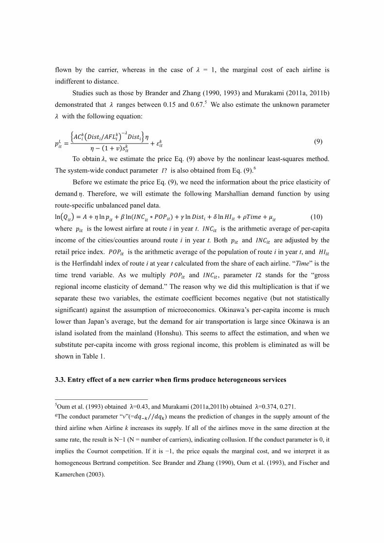
ln β β ln β ln β ln β ln β β

β β β β β

β

(28)

where is the origin-destination distance that is not affected by carrier or time. is

the fright frequency of each carrier k at route i in year t. is the

population-weighted-average of per-capita income, and is the weighted average of

populations of origin-destination cities or county areas around the main cities. The functional

form of these two variables are quadratic, and these forms were selected by comparing

log-likelihood functions of log-linear, log-linear of gross regional income (=ln( ∗ )

and linear-quadratic. , , , and are the carrier-specific fixed-effect

dummy variables to demonstrate the dynamic behavior of FSAs against new carriers’ entries.

The benchmark markets of these carrier-specific dummy variables are those without new

carriers’ entries; that is, one-year before new carriers’ entries and one-year after their exits.

Therefore, we expect the parameter of FSAs’ carrier-specific dummy variables will be positive.

According to our proposition in section 3.3, the effect of increasing * on new carriers’

outputs is negative, as long as FSAs successfully create their markets. However, the effect of

increasing * on airfares are not necessarily negative due to the effect of “shift-up” of

demand curve, that is, the positive sign of the parameters of carrier-specific dummy variables in

the demand function.

4. The Data

We used the data of Japanese domestic routes from 1998 to 2008. The total number of

routes is 14. The period of data for each route depends on the timing at which new carriers

entered. We chose the period from one year before the new entry to one year after the exit years.

For example, Tokyo-Miyazaki’s data starts from the year 2002 to 2008 because SNA had

entered in 2003 and it still continues to serve. The total number of samples is 222.

The data sources for available ton-kilometer, the operating costs of each carrier, the flight

distances, and the number of flights are the Koku Tokei Yoran (JAA Civil Aviation Handbook)

issued by the Japan Aeronautic Association and the website of each airline. The passenger data

and the distance of each route were obtained from the Koku Yuso Tokei Nempo (Yearly

Statistical Survey of Japanese Aviation) published by the Ministry of Land, Infrastructure and

Transport and Tourism. The fare information was obtained from the Jikoku Hyo (a timetable of

railways and airlines that is issued monthly by the Japan Tourist Bureau).

The demographic data sources such as population, income, and retail price index are from

the Kakei Chosa Hokoku (Family Income and Expenditure Survey), which is published by the

Japan Statistics Bureau, and the websites of the relevant prefectures and cities.

Passengers, numbers of flights, population and income are monthly data; we used April’s

data from each year, when the airline demand is the lowest in Japan. When evaluating the

lowest-demand month, we observed that the carriers issue various types of discount airfares to

generate demand. By choosing April, then, we can analyze the carriers that were most

competitive each year. The lists of routes and descriptive statistics are shown in Appendix 1

and Appendix 2, respectively.

5. Empirical Results and discussin

The estimation results of Eq. (7) are shown in Table 1. We estimated them by OLS

with heterocedasticity robust standard errors. The data are the route-specific unbalanced panel

data of 14 routes for 2–11 years.

Table 1. The estimated parameters of Eq. (10)

Variable Estimated Coefficient T-Ratio Price elasticity (η) −0.839 −2.562* Per-capita income*population (β） 1.381 4.124** Distance (γ) 2.038 4.659** Herfindahl index (δ) −1.140 −3.409** Time trend (ρ) −0.041 −1.486 Constant (A) −25.692 −1.936 Log likelihood function= −78.670, n = 76

Note: ** and * = significant at the 1% and 5% levels, respectively.

The price elasticity of demand (η) is −0.839, which was significant at the 5% level. Then,

using the estimated η, we further estimate λ and the system-wide conduct parameter ν. The data

used to estimate the Eq. (9) are different from those used for the estimation of Eq. (10). They are

the carrier-specific unbalanced panel data of 2 to 5 carriers in 14 routes for 2–11 years. Using

the nonlinear least-squares method, we obtain the estimated results shown in Table 2.

Table 2. The estimated parameters of Eq. (9)

Coefficient Estimated Coefficient T-Ratio

λ 0.216 13.671 ν 0.018 6.820 Log-likelihood function= −2548.48, n = 222

Note: Both parameters are significant at the 1% level.

The parameter λ is 0.216, which rejects the null hypothesis that λ equals 0 at the 1% level. The

system-wide conduct parameter ν is 0.018. This value is very close to the Cournot-competition

hypothesis, but is rejected at the 1% level of significance. Therefore, the system-wide fashion of

competition in Japanese domestic air markets falls between the Cournot fashion and collusion.

Comparing this result with Murakami (2011a), who found that ν was −0.242, Japanese airlines

are less competitive than before, since the “latecomer” carriers, SNA and SFJ, chose to soften

their competition compared to the first comers, that is, ADO and SKY.

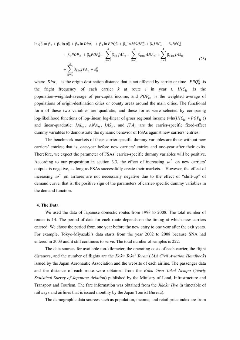
Next, we discuss the empirical results of the structural equation model in Table 3.

Table 3. Estimation results of the structural equations Inverse quasi-supply (=airfare) function Demand function

Variable Name Estimated Coefficient T-Ratio Variable Name Estimated

Coefficient T-Ratio

Passenger −0.038 −2.474* Air fare −0.762 −5.594**

Marginal cost 0.656 12.170** Distance 0.605 4.033** Share 0.111 4.359** Frequency 1.133 30.94**

JAL−JAS merger 0.178 5.450** Share 0.177 3.907**

JAL exit 0.017 0.209 Income −97.077 −0.738ANA exit −0.055 −0.525 Income2 3.725 0.734JAS exit −0.142 −1.098 Population −21.976 −2.135*

ADO exit 0.524 2.079* Population2 0.735 2.137*

ADO 1st year −0.658 −3.644** JAL 1st year 0.170 2.041*

ADO 2nd year −0.404 −3.157** JAL 2nd year 0.165 1.866ADO 3rd year −0.269 −2.113* JAL 3rd year 0.086 0.834ADO 4th year −0.169 −2.647** JAL 4th year 0.122 1.557SKY 1st year −0.532 −7.419** ANA 1st year 0.234 2.676**

SKY 2nd year −0.418 −5.801** ANA 2nd year 0.250 2.521*

SKY 3rd year −0.290 −3.557** ANA 3rd year 0.250 2.094*

SKY 4th year −0.249 −4.015** ANA 4th year 0.247 3.049**

SNA 1st year −0.215 −1.998* JAS 1st year 0.176 1.345SNA 2nd year −0.243 −1.883 JAS 2nd year 0.056 0.387SNA 3rd year −0.141 −1.086 JAS 3rd year 0.192 0.954SNA 4th year −0.311 −2.843** JAS 4th year 0.257 1.247SFJ 1st year −0.205 −1.604 JTA 1st year −0.076 −0.250SFJ 2nd year −0.168 −0.927 JTA 2nd year −0.026 −0.086SFJ 3rd year −0.004 −0.021

Constant 3.877 7.054 Constant 803.990 0.950

Note: ** and * = significant at the 1% and 5% levels, respectively. System R2=0.973, R2 of

quasi-supply=0.622, R2 of demand=0.916, n=222, estimated by Iterated 3SLS.

The endogenous variables are specified as airfare and price, so the model is

over-identified. As for the quasi-supply, the parameter ‘passengers’ is slightly negative. This

implies that economies of density exist. The first two new carriers discounted their airfares

significantly for the first four years of entries, unlike the two latecomers, but airfare levels have

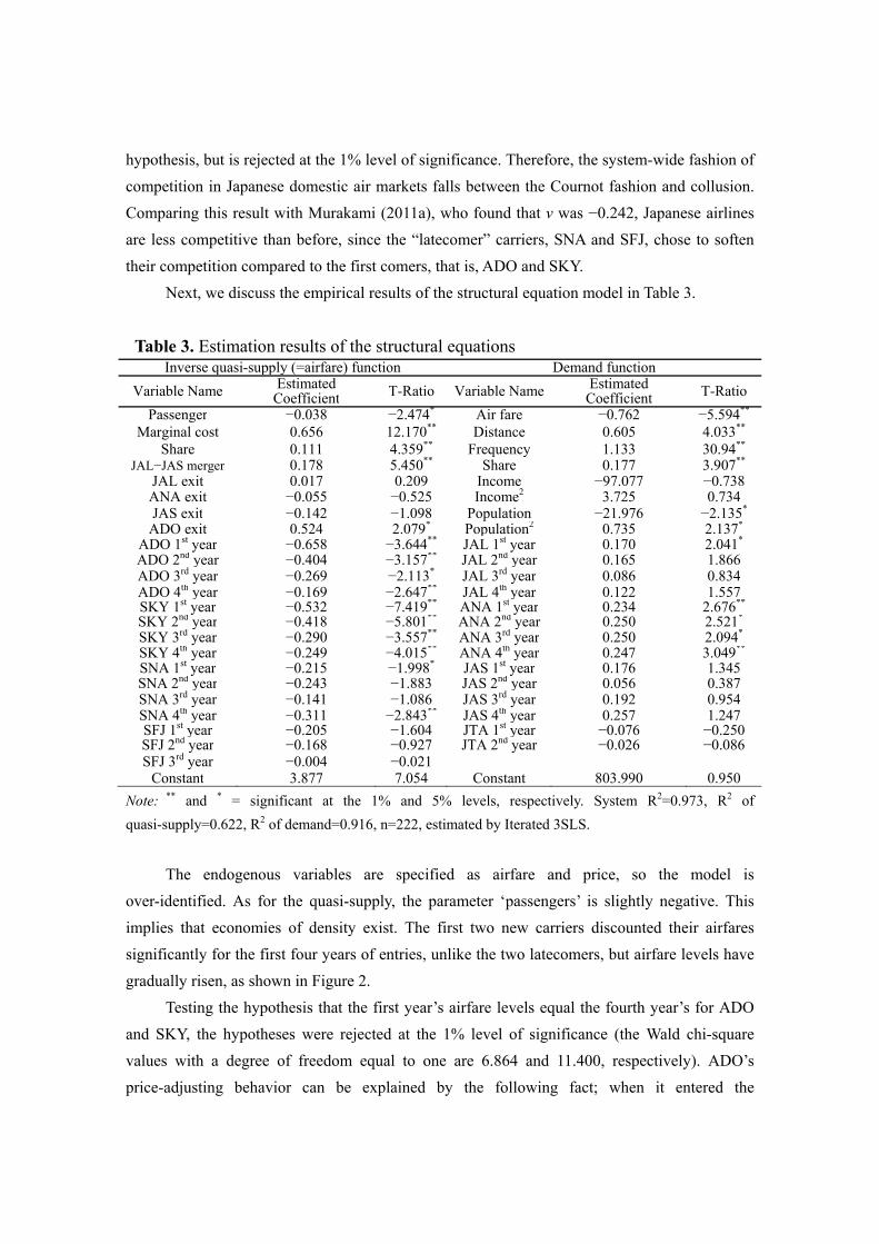
gradually risen, as shown in Figure 2.

Testing the hypothesis that the first year’s airfare levels equal the fourth year’s for ADO

and SKY, the hypotheses were rejected at the 1% level of significance (the Wald chi-square

values with a degree of freedom equal to one are 6.864 and 11.400, respectively). ADO’s

price-adjusting behavior can be explained by the following fact; when it entered the

Tokyo-Sapporo market in 1998, it was a budget carrier fully independent of the FSAs, but after

it went bankrupt and then revived under the codeshare agreement with ANA, ADO stopped

offering aggressive discounts. SKY has been independent of FSAs since its founding in 1996

(the first entry was in 1998) as of now, but its price-adjusting behavior is quite similar to

ADO’s.

Fig. 2. Overtime changes in the airfares of new Japanese carriers.

Note: The airfares were adjusted by retail price index (chain of average).

During the period we analyzed, SKY seems to have faced the same situation as ADO, but

unlike the case of ADO, SKY was saved by a large investment from an individual entrepreneur

who managed an internet service provider.7

Regarding the carrier-exit dummy variables, the FSAs did not raise airfares after their

rivals exited, but ADO did. This means that ADO is not a U.S.-type LCC like Southwest

Airlines in the 1990s that kept airfares at low levels, but rather is similar to FSAs.

In the demand function, the signs of ANA’s fixed-effect dummy variables are consistently

positive, and JAL’s first year is also positive and significant. Considering our Proposition, ANA

successfully created different markets against the entry of new carriers, but other FSAs did not

necessarily do so. When we derive the reduced form of demand function, new carriers’

parameters are also positive, and this result is contrary to the assumption of FSAs’ creation of

new markets. Considering this result and the unstable parameters of FSAs, only ANA succeeded

in distinguishing itself compared with other FSAs.

Our final analysis is how the consumers’ surplus changed from the first year of entries by

new carriers to the fourth year. Table 4 shows the increase or decrease in the consumers’ surplus

on year by year and carrier by carrier bases. The method of computation is to use the estimated

demand function and calculate the change in the triangle surrounded by the intercept of inverse

7The Nikkei, September 24th, 2003.

-0.700

-0.600

-0.500

-0.400

-0.300

-0.200

-0.100

0.0001st year 2nd year 3rd year 4th year

ADO

SKY

SNA

SFJ

demand, the average airfare of each carrier, and the corresponding quantities of each carrier.

Therefore, what is derived was is the size of trapezoids (=increase or decrease in consumers’

surplus).

Table 4. Change in consumers’ surplus after new entries of carriers

1st year 2nd year 3rd year 4th year Total JAL 362.51 351.77 182.72 259.61 1156.61ANA 583.82 624.17 624.17 616.60 2448.75JAS 229.73 72.71 250.79 336.64 889.88JTA −12.57 −4.31 −16.88ADO 553.68 337.12 223.47 139.93 1254.20SKY 359.11 281.10 194.20 166.52 1000.93SNA 96.54 109.21 63.15 140.08 408.98SFJ 156.21 127.86 3.03 287.09

TOTAL 2329.02 1899.63 1541.53 1659.38 7429.57

Note: 1,000USD (1 USD = 100 Yen).

Overall, the first-year impacts were the largest, and the impacts gradually got weaker.

However, the consumers’ surplus was apparently increased by the new entries. From the

viewpoint of consumers’ protection, the introduction of the policy allowing new carriers’ entries

was successful. However, it must be noted that this result may have come from the large

increase in consumes’ surplus in two large markets, Tokyo-Sapporo and Tokyo-Fukuoka.

Looking at the results of JTA and SFJ (which are comparatively small carriers), our concern is

that small communities might not have benefited or benefited only slightly from the policy.8

Another concern is that the merger of JAL and JAS generated a $230,000 USD loss of

consumers’ surplus in the merger year. More attention should be paid to merging carriers, and

forecasts of the welfare gain or loss will be needed.

6. Conclusions

The outstanding features of our analyses are that we modeled the effect of market

separation on the outputs of carriers and empirically found that the border of market separation

was ambiguous, that new entries improved the consumers’ surplus of large markets, seemingly,

and that the first-year impact on the improvement of the consumers’ surplus was largest and

then gradually declined. From the perspective of consumers’ welfare, it would be better to leave

ambiguous the border of market separation between FSAs and new carriers and to let

8JTA connects the mainland (Honshu) and Okinawa and flies between islands in Okinawa. SFJ was based at Kita-Kyushu Airport during this examination period and connected Kita-Kyushu City and Tokyo. Kita-Kyushu City is in Fukuoka Prefecture, but the Tokyo-Kitakyushu market is much smaller than the Tokyo-Fukuoka market.

passengers move between FSAs and new carriers, since the market separation enforces the

increase in FSAs’ output; this would lead to enhancement of the monopolistic power of FSAs.

We also need to let new entrants maintain their airfare levels in the long run. To do this, we need

to open the slots of large airports to new entrants and bring up the new entrants so that they can

survive the airfare competition with FSAs.

The limitations of our paper are that (1) we could not cover the period during which JAL

changed their disclosure method, and (2) we did not include Japanese LCCs such as Peach

Aviation, Jetstar Japan and Air Asia Japan due to the unavailability of data. These drawbacks

will be eliminated by our future research.

Appendix 1. The route list used for estimation

Appendix 2. Descriptive statistics

References

Alderighi, M., A. Cento, P. Nijkamp, and P. Rietveld, 2004. The entry of low-cost airlines: price

competition in the European airline market, Tinbergen Institute discussion paper, TI 04-074/3.

Brander, J. A., and A. Zhang, 1990. Market conduct in the airline industry: An empirical investigation,

RAND Journal of Economics 21, 567-583.

Brander, J. A., and A. Zhang, 1993. Dynamic oligopoly behavior in the airline industry, International

Route Period Distance (km) Carrier (period) SampleTokyo-Sapporo 1998-2008 894 JAL(98-08) ANA(98-08) JAS(98-02) ADO(99-08) SKY(06-08) 40

Tokyo-Fukuoka 1998-2008 1041 JAL(98-08) ANA(98-08) JAS(98-02) SKY(99-08) 37

Osaka-Sapporo 1998-2001 1161 JAL(98-01) ANA(98-01) JAS(98-01) SKY(00) 13

Osaka-Fukuoka 1998-2001 578 JAL(98-01) ANA(98-01) JAS(99-01) SKY(99-00) 13Tokyo-Asahikawa 2003-2008 1052 JAL(03-08) ANA(03) ADO(04-08) SKY(08) 13

Tokyo-Aomori 2002-2004 690 JAL(03-04) ANA(02-03) JAS(02) SKY(03) 6

Tokyo-Tokushima 2002-2007 703 JAL(03-07) ANA(02-03) JAS(02) SKY(03-06) 12

Tokyo-Miyazaki 2002-2008 1023 JAL(02-08) ANA(02-08) JAS(02) SNA(03-08) 21Tokyo-Kagoshima 2001-2008 1111 JAL(01-08) ANA(01-08) JAS(01-02) SKY(02-06) SNA(08) 24

Tokyo-Kobe 2006-2008 695 JAL(06-08) ANA(06-08) SKY(06-08) 9

Tokyo-Kitakyushu 2005-2008 958 JAL(05-08) SFJ(06-08) 7

Tokyo-Osaka 2007-2008 678 JAL(07-08) ANA(07-08) SFJ(08) 5

Tokyo-Nagasaki 2005-2008 1143 JAL(05-08) ANA(05-08) SNA(06-08) 11Tokyo-Okinawa 2006-2008 1687 JAL(06-08) ANA(06-08) JTA(06-08) SKY(07-08) 11

Number of Routes = 14, Number of Samples = 222

Variable Name Mean Standard Error Minimum Maximum MedianDistance 985.450 15.559 578.000 1109.000 1023.000Passenger 88433.982 5731.941 1599.000 324299.000 53069.000

Price 26787.838 497.385 9600.000 40800.000 28000.000Price (lowest) 23946.396 490.321 9600.000 40800.000 23000.000

Poplation 3944138.636 54251.184 1966125.798 4936713.245 4100038.640Income 2010057.529 127487.364 369972.647 4578925.465 432980.034Share 34.234 1.290 1.463 100.000 35.569

Journal of Industrial Organization 11, 407-435.

Caves, D. W., L. R. Chistensen, and M. W. Tretheway, 1984. Economies of density versus economies of

scale: Why trunk and local service airline costs differ, RAND Journal of Economics, 15, 471-489.

Dresner, M., J. S. C. Lin, and R. Windle, 1996. The impact of low-cost carriers on airport and route

competition, Journal of Transport Economics and Policy, 30(3), 309-328.

Fischer T. and D. R. Kamerschen, 2003. Price-cost margins in the US airline industry using a conjectural

variation approach, Journal of Transport Economics and Policy, 37(2), 227-259.

Fu, X., M. Dresner, and T.H. Oum, 2011. Effects of transport service differentiation in the US domestic

airline market, Transportation Research Part E,47(3), 297-305.

Gillen D. W., T. H. Oum and M. W. Tretheway, 1990. Airline cost structure and policy implications: A

multi-product approach for Canadian airlines, Journal of Transport Economics and Policy, 24(1),

9-33.

Goolsbee, A. and C. Syverson, 2005. How do incumbents respond to the threat of entry?: evidence from

the major airlines, NBER Working Paper, 11072.

Johnston, A. and J.Ozment, 2013. Economies of scale in the US airline industry. Transportation Research

Part E, 51, 95-108.

Morrison, S. A. and C. Winston, 1996. Evolution of Airline Industry, Brookings Institution, Chaper 4.

Morrison, S. A., 2001, Actual, adjacent, and potential competition: Estimating the full effect of Southwest

Airlines, Journal of Transport Economics and Policy, 35, 239-256.

Murakami, H.,2011a, An empirical analysis of inter-firm rivalry between Japanese full-service and

low-cost carriers, Pacific Economic Review, 16(1), 103-119.

Murakami, H.,2011b,Time effect of low-cost carrier entry and social welfare in US large air markets,

Transportation Research Part E, 47(3), 306-314

Murakami, H. and R. Asahi, 2011. An empirical analysis of the effect of multimarket contacts on US air

carriers' pricing behaviors, Singapore Economic Review, 56(4), 593-600.

Oliveira, A.V.M., and C. Huse,, 2009, Localized competitive advantage and price reactions to entry: Full-

service vs. low-cost airlines in recently liberalized emerging markets, Transportation Research Part E,

45(2), 307-320.

Oum, T. H., A. Zhang., and Y. Zhang, 1993. Inter-firm rivalry and firm-specific price elasticities in the

deregulated airline markets, Journal of Transport Economics and Policy, 27, 171-192.

Pitfield, D.E., 2005. Some speculations and empirical evidence on the oligopolistic behavior of

competing low-cost airlines,” Journal of Transport Economics and Policy, 39(3), 379-390.

Pitfield, D.E., 2008. The Southwest effect: A time-series analysis on passengers carried by selected routes

and a market share comparison, Journal of Air Transport Management, 14(3), 113-122.

Vowles, T. W., 2000, “The effect of low fare air carriers on airfares in the US”, Journal of Transport

Geography, 8, 121-128. [2013.8.28 1140]