Embed Size (px)
Citation preview

5/13/2018 2012.CFA.L1.Formula.sheet (1) - slidepdf.com
http://slidepdf.com/reader/full/2012cfal1formulasheet-1 1/73
ECONOMICAL EFFICIENT EFFECTIVE
ÉLANGUIDES
We believe that we offer the MOST EFFECTIVE study materials for CFA exam prep.Register for the free trial on our website to obtain FREE access to the following studymaterials.
Lecture videos, study guide readings and practice questions for Study Session 3(Quantitative Methods)
Lecture videos, study guide readings and practice questions for Study Session 16(Fixed Income)
Our products receive excellent reviews from customers. Sign up for our free trial nowto experience the difference that we can make to your CFA level I Prep.
40% Discount for Retakers.40% Discount for Full-Time Students.
Thousands of customers from
more than 80countries
around theworld have usedElan Guides toprepare for the
CFA Level Iexam.

5/13/2018 2012.CFA.L1.Formula.sheet (1) - slidepdf.com
http://slidepdf.com/reader/full/2012cfal1formulasheet-1 2/73
WHY USE ÉLAN GUIDES
Member of CFA Institute PrepProvider Guidelines Program
Video instruction (approx hrs)
Faculty Email Utility/ExpertGuidance
LOS Trackers
Prices
Study NotesLecture VideosReview BookPractice Questions
Discounts for retakers
Offers electronic versions of study materials
Offers individual videos andreadings for sale
Élan Guides
Yes
70
For all customers
Yes
$150$300$50
$150(2000 questions)
For every retakerincluding those who
have never usedÉlan Guides before
Applicable on eachand every product
and package
Yes
Yes
Kaplan Schweser
Yes
50
Only for customers
who purchase
packages worth
$599 or more
No
$299$499
$99
$299
(4000 questions)
Only if you buy a
package worth $599
or more
Only applicable on
packages worth
$999 or more
No
No
Stalla
Yes
60
Only for customers
who purchase
packages worth
$1,590
No
$350N/A*
$50
$350
(4000 questions)
Only for those who
have used Stalla
before
Stalla Promise
available if you buy
a package worth
$999 or more
No
No
* Not available as a stand-alone product
“I used Elan's study materials for the June 2011 Level I test and was highly impressed by the quality of the practice tests andexplanations, lecture videos, and study notes... as well as your quick replies when I had questions on my order. I would very muchlike to continue using Elan study materials as I work through the CFA curriculum and hope that you have found enough successto expand your offerings.” – Paul, USA
“Without really commenting on the quality of the others stuff, I must say that I found you guys to be the best.”- Sheila, Saudi Arabia
“You guys really do make a superior product and provide a better service in pretty much every way. Like I have said before, yourmaterials really are top quality. Thanks again for all your hard work. I have been consistently doing better on all my practiceexams since I switched over to your materials.”– Bijan, USA

5/13/2018 2012.CFA.L1.Formula.sheet (1) - slidepdf.com
http://slidepdf.com/reader/full/2012cfal1formulasheet-1 3/73
QUANTITATIVE METHODS
FVN = PV (1+ r)N
PV = FV
(1+ r)N
PVAnnuity Due = PVOrdinary Annuity (1 + r)
FVAnnuity Due = FVOrdinary Annuity (1 + r)
PV(perpetuity) =PMT
I/Y
FVN = PVe rs * N
EAR = (1 + Periodic interest rate)N- 1
where:
rBD = the annualized yield on a bank discount basis.
D = the dollar discount (face value – purchase price)
F = the face value of the bill
t = number of days remaining until maturity
rBD =D
360
F t
where:
P0 = initial price of the investment.
P1 = price received from the instrument at maturity/sale.
D1 = interest or dividend received from the investment.
HPY = P1 - P0 + D1 = P1 + D1 - 1
P0 P0
where
CFt = the expected net cash flow at time t
N = the investment’s projected life
r = the discount rate or appropriate cost of capital
CFt
(1 + r)t
t=0
NNPV =
Net Present Value
Bank Discount Yield
Holding Period Yield
The Future Value of a Single Cash Flow
The Present Value of a Single Cash Flow
Present Value of a Perpetuity
Continuous Compounding and Future Values
Effective Annual Rates
© 2011 ELAN GUIDES 3
QUANTITATIVE METHODS
5/13/2018 2012.CFA.L1.Formula.sheet (1) - slidepdf.com
http://slidepdf.com/reader/full/2012cfal1formulasheet-1 4/73
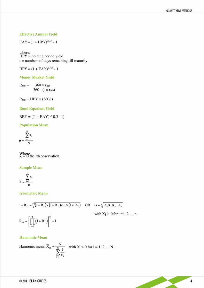
EAY= (1 + HPY)365/t - 1
where:HPY = holding period yield
t = numbers of days remaining till maturity
RMM = HPY (360/t)
RMM = 360 rBD
360 - (t rBD)
HPY = (1 + EAY)t/365 - 1
BEY = [(1 + EAY) ^ 0.5 - 1]
Where,xi = is the ith observation.
with Xi > 0 for i = 1, 2,..., N.
Effective Annual Yield
Money Market Yield
Bond Equalent Yield
Population Mean
Sample Mean
Geometric Mean
Harmonic Mean
© 2011 ELAN GUIDES 4
QUANTITATIVE METHODS

5/13/2018 2012.CFA.L1.Formula.sheet (1) - slidepdf.com
http://slidepdf.com/reader/full/2012cfal1formulasheet-1 5/73
Range = Maximum value - Minimum value
Where:
n = number of items in the data set
= the arithmetic mean of the sample
where:
y = percentage point at which we are dividing the distribution
Ly = location (L) of the percentile (Py) in the data set sorted in ascending order
where:
Xi = observation i
= population mean
N = size of the population
Percentiles
Range
Mean Absolute Deviation
Population Variance
Population Standard Deviation
where:
n = sample size.
Sample variance =
Sample Variance
© 2011 ELAN GUIDES 5
QUANTITATIVE METHODS

5/13/2018 2012.CFA.L1.Formula.sheet (1) - slidepdf.com
http://slidepdf.com/reader/full/2012cfal1formulasheet-1 6/73
where:
= mean portfolio return
= risk-free return
= standard deviation of portfolio returns
s
s
where:
s = sample standard deviation
= the sample mean.
Coefficient of variation
Sample Standard Deviation
Coefficient of Variation
Sharpe Ratio
SK =
n
i = 1
(Xi - X)3
s3
n
(n - 1)(n - 2)[ ]
As n becomes large, the expression reduces to the mean cubed deviation.
where:
s = sample standard deviation
n
n
i = 1
(Xi - X)3
s3
SK
Sample skewness, also known as sample relative skewness, is calculated as:
© 2011 ELAN GUIDES 6
QUANTITATIVE METHODS

5/13/2018 2012.CFA.L1.Formula.sheet (1) - slidepdf.com
http://slidepdf.com/reader/full/2012cfal1formulasheet-1 7/73
Where the odds for are given as ‘a to b’, then:
Odds for an event
Where the odds against are given as ‘a to b’, then:
Odds for an event
Sample Kurtosis uses standard deviations to the fourth power. Sample excess kurtosis is
calculated as:
For a sample size greater than 100, a sample excess kurtosis of greater than 1.0 would be
considered unusually high. Most equity return series have been found to be leptokurtic.
KE =
n
i = 1
(Xi - X)4
s4
n(n + 1)
(n - 1)(n - 2)(n - 3)( ) 3(n - 1)2
(n - 2)(n - 3)
where:
s = sample standard deviation
n
n
i = 1
(Xi - X)4
s4
KE 3
As n becomes large the equation simplifies to:
© 2011 ELAN GUIDES 7
QUANTITATIVE METHODS

5/13/2018 2012.CFA.L1.Formula.sheet (1) - slidepdf.com
http://slidepdf.com/reader/full/2012cfal1formulasheet-1 8/73
P(A or B) = P(A) + P(B) - P(AB)
P(A and B) = P(A) P(B)
Expected Value
Where:
Xi = one of n possible outcomes.
n
i=1
P(A) = P(AS) + P(ASc)
P(A) = P(A|S) P(S) + P(A|Sc) P(Sc)
P(A) = P(A|S1) P(S1) + P(A|S2) P(S2) + ...+ P(A|Sn) P(Sn)
where the set of events {S1, S2,..., Sn} is mutually exclusive and exhaustive.
The Total Probability Rule
Conditional Probabilities
Multiplication Rule for Probabilities
Addition Rule for Probabilities
For Independant Events
P(A|B) = P(A), or equivalently, P(B|A) = P(B)
The Total Probability Rule for n Possible Scenarios
© 2011 ELAN GUIDES 8
QUANTITATIVE METHODS

5/13/2018 2012.CFA.L1.Formula.sheet (1) - slidepdf.com
http://slidepdf.com/reader/full/2012cfal1formulasheet-1 9/73
Variance and Standard Deviation
2(X) = E{[X - E(X)]
2}
n
i=1
2(X) = P(Xi) [Xi - E(X)]
2
1. E(X) = E(X|S)P(S) + E(X|Sc)P(Sc)
2. E(X) = E(X|S1) P(S1) + E(X|S2) P(S2) + ...+ E(X|Sn) P(Sn)
Where:
E(X) = the unconditional expected value of X
E(X|S1) = the expected value of X given Scenario 1P(S1) = the probability of Scenario 1 occurring
The set of events {S1, S2,..., Sn} is mutually exclusive and exhaustive.
Cov (XY) = E{[X - E(X)][Y - E(Y)]}
Cov (RA,RB) = E{[RA - E(RA)][RB - E(RB)]}
Correlation Coefficient
Corr (RA,RB) = (RA,RB) =
Cov (RA,RB)
(A)(B)
The Total Probability Rule for Expected Value
Covariance
Expected Return on a Portfolio
Where:
Portfolio Variance
Variance of a 2 Asset Portfolio
© 2011 ELAN GUIDES 9
QUANTITATIVE METHODS

5/13/2018 2012.CFA.L1.Formula.sheet (1) - slidepdf.com
http://slidepdf.com/reader/full/2012cfal1formulasheet-1 10/73
Bayes’ Formula
The number of different ways that the k tasks can be done equals n1 n2 n3 …nk .
Remember: The combination formula is used when the order in which the items are assigned the
labels is NOT important.
Permutations
Counting Rules
Combinations
Variance of a 3 Asset Portfolio
F(x) = n p(x) for the nth observation.
Discrete uniform distribution
Binomial Distribution
where:
p = probability of success
1 - p = probability of failure
= number of possible combinations of having x successes in n trials. Stated differently, it is the number
of ways to choose x from n when the order does not matter.
Variance of a binomial random variable
© 2011 ELAN GUIDES 10
QUANTITATIVE METHODS

5/13/2018 2012.CFA.L1.Formula.sheet (1) - slidepdf.com
http://slidepdf.com/reader/full/2012cfal1formulasheet-1 11/73
Minimize P(RP< RT)
where:
RP = portfolio return
RT = target return
Roy’s safety-first criterion
= continuously compounded annual rate
Continuously Compounded Returns
The 90% confidence interval is
The 95% confidence interval is
The 99% confidence interval is
- 1.65s to
- 1.96s to
- 2.58s to
+ 1.65s
+ 1.96s
+ 2.58s
For a random variable X that follows the normal distribution:
The following probability statements can be made about normal distributions
Approximately 50% of all observations lie in the interval Approximately 68% of all observations lie in the interval Approximately 95% of all observations lie in the interval Approximately 99% of all observations lie in the interval
Confidence Intervals
z = (observed value - population mean)/standard deviation = (x – )/
z-Score
Shortfall Ratio
The Continuous Uniform Distribution
P(X < a), P (X >b) = 0
x2 -x1
b - aP (x1 X x2 ) =
© 2011 ELAN GUIDES 11
QUANTITATIVE METHODS

5/13/2018 2012.CFA.L1.Formula.sheet (1) - slidepdf.com
http://slidepdf.com/reader/full/2012cfal1formulasheet-1 12/73
where:
= the standard error of the sample mean
= the population standard deviation
n = the sample size
= standard error of sample mean
s = sample standard deviation.
where:
Point estimate (reliability factor standard error)
where:
Point estimate = value of the sample statistic that is used to estimate the population
parameter
Reliability factor = a number based on the assumed distribution of the point
estimate and the level of confidence for the interval (1- ).
Standard error = the standard error of the sample statistic (point estimate)
where:
= The sample mean (point estimate of population mean)z /2 = The standard normal random variable for which the probability of an
observation lying in either tail is / 2 (reliability factor).
= The standard error of the sample mean.n
= sample mean (the point estimate of the population mean)
= standard error of the sample mean
s = sample standard deviation
where:
= the t-reliability factor
Standard Error of Sample Mean when Population variance is Known
Standard Error of Sample Mean when Population variance is Not Known
Confidence Intervals
Sampling error of the mean = Sample mean - Population mean =
Sampling Error
© 2011 ELAN GUIDES 12
QUANTITATIVE METHODS

5/13/2018 2012.CFA.L1.Formula.sheet (1) - slidepdf.com
http://slidepdf.com/reader/full/2012cfal1formulasheet-1 13/73
Sample statistic - Hypothesized value
Standard error of sample statisticTest statistic =
Power of a test = 1 - P(Type II error)
[ ]( )sample
statistic
critical
value
standard
error
population
parameter- ( ) ( ) ( ) ( )sample
statistic+ ]critical
value
standard
error) ( )([x - (z) µ0 x + (z)( ) ( )
Test Statistic
Power of a Test
Confidence Interval
Decision
Do not reject H0
Reject H0
H0 is True
Correct decision
Incorrect decision
Type I error
Significance level =
P(Type I error)
H0 is False
Incorrect decision
Type II error
Correct decision
Power of the test
= 1 - P(Type II
error)
Decision Rules for Hypothesis Tests
Type of test
One tailed
(upper tail)
test
One tailed
(lower tail)
test
Two-tailed
Null
hypothesis
H0 : µ µ0
H0 : µ µ0
H0 : µ =µ0
Alternate
hypothesis
Ha : µ µ0
Ha : µ µ0
Ha : µ µ0
Reject null if
Test statistic >
critical value
Test statistic <
critical value
Test statistic <
Lower critical
value
Test statistic >
Upper critical
value
Fail to reject
null if
Test statistic critical value
Test statistic critical value
Lower critical
value test
statistic Upper critical
value
P-value represents
Probability that lies
above the computed
test statistic.
Probability that lies
below the computed
test statistic.
Probability that lies
above the positive
value of the computed
test statistic plus the
probability that lies
below the negative
value of the computed
test statistic
Summary
© 2011 ELAN GUIDES 13
QUANTITATIVE METHODS

5/13/2018 2012.CFA.L1.Formula.sheet (1) - slidepdf.com
http://slidepdf.com/reader/full/2012cfal1formulasheet-1 14/73
Tests for Means when Population Variances are Assumed Equal
Where:
2s1 = variance of the first sample
n2 = number of observations in second sample
n1 = number of observations in first sample
degrees of freedom = n1 + n2 -2
2
s2 = variance of the second sample
Where:
x = sample mean
µ0= hypothesized population mean
= standard deviation of the population
n = sample size
z-stat =x - µ0
t-stat =x - µ0
Where:
x = sample mean
µ0= hypothesized population mean
s = standard deviation of the sample
n = sample size
z-stat =x - µ0
Where:
x = sample mean
µ0= hypothesized population mean
s = standard deviation of the sample
n = sample size
t-Statistic
z-Statistic
© 2011 ELAN GUIDES 14
QUANTITATIVE METHODS

5/13/2018 2012.CFA.L1.Formula.sheet (1) - slidepdf.com
http://slidepdf.com/reader/full/2012cfal1formulasheet-1 15/73
Tests for Means when Population Variances are Assumed Unequal
t-stat
2s1 = variance of the first sample
n2 = number of observations in second sample
n1 = number of observations in first sample
2s2 = variance of the second sample
Where:
Where:
d = sample mean difference
sd = standard error of the mean difference=
sd = sample standard deviation
n = the number of paired observations
Paired Comparisons Test
Population
distribution
Normal
Normal
Normal
Relationship
between
samples
Independent
Independent
Dependent
Assumption
regarding
variance
Equal
Unequal
N/A
Type of test
t-test pooled
variance
t-test with
variance not
pooled
t-test with
paired
comparisons
Hypothesis Tests Concerning the Mean of Two Populations - Appropriate Tests
© 2011 ELAN GUIDES 15
QUANTITATIVE METHODS

5/13/2018 2012.CFA.L1.Formula.sheet (1) - slidepdf.com
http://slidepdf.com/reader/full/2012cfal1formulasheet-1 16/73
Where:
n = sample size
s2 = sample variance
= hypothesized value for population variance20
Where:
= Variance of sample drawn from Population 1
= Variance of sample drawn from Population 2
2s1
2s2
Chi Squared Test-Statistic
Test-Statistic for the F-Test
Hypothesis tests concerning the variance.
Hypothesis Test Concerning
Variance of a single, normally distributed
population
Equality of variance of two independent,
normally distributed populations
Appropriate test statistic
Chi-square stat
F-stat
Setting Price Targets with Head and Shoulders Patterns
Price target = Neckline - (Head - Neckline)
Setting Price Targets for Inverse Head and Shoulders Patterns
Price target = Neckline + (Neckline - Head)
Momentum or Rate of Change Oscillator
M = (V - V x) 100
where:M = momentum oscillator value
V = last closing price
V x = closing price x days ago, typically 10 days
© 2011 ELAN GUIDES 16
QUANTITATIVE METHODS

5/13/2018 2012.CFA.L1.Formula.sheet (1) - slidepdf.com
http://slidepdf.com/reader/full/2012cfal1formulasheet-1 17/73
Relative Strength Index
RSI = 100 1 + RS
100
where RS = (|Down changes for the period under consideration|)
(Up changes for the period under consideration)
Stochastic Oscillator
%K = 100 ( H14 L14
C L14 )where:
C = last closing price
L14 = lowest price in last 14 days
H14 = highest price in last 14 days
%D (signal line) = Average of the last three %K values calculated daily.
Short interest ratio = Average daily trading volume
Short interest
Short Interest ratio
Arms Index
Arms Index =Volume of advancing issues / Volume of declining issues
Number of advancing issues / Number of declining issues
© 2011 ELAN GUIDES 17
QUANTITATIVE METHODS

5/13/2018 2012.CFA.L1.Formula.sheet (1) - slidepdf.com
http://slidepdf.com/reader/full/2012cfal1formulasheet-1 18/73
ECONOMICS
DEMAND AND SUPPLY ANALYSIS: INTRODUCTION
Demand function: QDx = f(Px, I, Py, . . .) … (Equation 1)
The demand function captures the effect of all these factors on demand for a good.
Equation 1 is read as “the quantity demanded of Good X (QDX) depends on the price of
Good X (PX), consumers’ incomes (I) and the price of Good Y (PY), etc.”
The supply function can be expressed as:
Supply function: QSx = f(Px, W, . . .) … (Equation 5)
The own-price elasticity of demand is calculated as:
… (Equation 16)EDPx =%QDx
%Px
If we express the percentage change in X as the change in X divided by the value of X,
Equation 16 can be expanded to the following form:
… (Equation 17)EDPx =%QDx
%Px
=
QDxQDx
PxPx
=QDx
Px( )
Px
QDx( )
Arc elasticity is calculated as:
EP =% change in quantity demanded
% change in price=
% Qd
% P
(Q0 - Q1)
(Q0 + Q1)/2100
(P0 - P1)
(P0 + P1)/2100
=
Slope of demand
function.
Coefficient on own-price in market
demand function
© 2011 ELAN GUIDES 18
ECONOMICS

5/13/2018 2012.CFA.L1.Formula.sheet (1) - slidepdf.com
http://slidepdf.com/reader/full/2012cfal1formulasheet-1 19/73
Cross-Price Elasticity of Demand
Cross elasticity of demand measures the responsiveness of demand for a particular good to
a change in price of another good, holding all other things constant.
EC =% change in quantity demanded
% change in price of substitute or complement
… (Equation 19)EDPy =%QDx
%Py
=
QDx QDx
PyPy
=QDx
Py( )
Py
QDx( )
Income Elasticity of Demand
Income elasticity of demand measures the responsiveness of demand for a particular good
to a change in income, holding all other things constant.
EI =% change in quantity demanded
% change in income
… (Equation 18)EDI =%QDx
%I=
QDxQDx
II
=QDx
I( )I
QDx( )
Same as coefficienton I in market
demand function(Equation 11)
Same as coefficienton PY in market
demand function(Equation 11)
© 2011 ELAN GUIDES 19
ECONOMICS

5/13/2018 2012.CFA.L1.Formula.sheet (1) - slidepdf.com
http://slidepdf.com/reader/full/2012cfal1formulasheet-1 20/73
DEMAND AND SUPPLY ANALYSIS: CONSUMER DEMAND
he Utility Function
In general a utility function can be represented as:
U = f(Qx1 , Qx
2 ,..., Qx
n)
DEMAND AND SUPPLY ANALYSIS: THE FIRM
Accounting Profit
Accounting profit (loss) = Total revenue – Total accounting costs.
Economic Profit
Economic profit (also known as abnormal profit or supernormal profit) is calculated as:
Economic profit = Total revenue – Total economic costs
Economic profit = Total revenue – (Explicit costs + Implicit costs)
Economic profit = Accounting profit – Total implicit opportunity costs
Normal Profit
Normal profit = Accounting profit - Economic profit
Total, Average and Marginal Revenue
Table 2: Summary of Revenue Terms 2
Revenue
Total revenue (TR)
Average revenue (AR)
Marginal revenue (MR)
Calculation
Price times quantity (P Q), or the sum of individual units
sold times their respective prices; (Pi Qi)
Total revenue divided by quantity; (TR / Q)
Change in total revenue divided by change in quantity; (TR
/ Q)
© 2011 ELAN GUIDES 20
ECONOMICS

5/13/2018 2012.CFA.L1.Formula.sheet (1) - slidepdf.com
http://slidepdf.com/reader/full/2012cfal1formulasheet-1 21/73
Total, Average, Marginal, Fixed and Variable Costs
Table 5: Summary of Cost Terms 3
Costs
Total fixed cost (TFC)
Total variable cost (TVC)
Total costs (TC)
Average fixed cost (AFC )
Average variable cost (AVC)
Average total cost (ATC)
Marginal cost (MC)
Calculation
Sum of all fixed expenses; here defined to include all
opportunity costs
Sum of all variable expenses, or per unit variable cost
times quantity; (per unit VC Q)
Total fixed cost plus total variable cost; (TFC + TVC)
Total fixed cost divided by quantity; (TFC / Q)
Total variable cost divided by quantity; (TVC / Q)
Total cost divided by quantity; (TC / Q) or (AFC + AVC)
Change in total cost divided by change in quantity;
(TC / Q)
2 Exhibit 3, pg 106, Volume 2, CFA Program Curriculum 2012
Marginal revenue product (MRP) of labor is calculated as:
MRP of labor = Change in total revenue / Change in quantity of labor
For a firm in perfect competition, MRP of labor equals the MP of the last unit of labor times
the price of the output unit.
MRP = Marginal product * Product price
A profit-maximizing firm will hire more labor until:
MRPLabor = PriceLabor
Profits are maximized when:
MRP1
Price of input 1
MRPn
Price of input n= ... =
© 2011 ELAN GUIDES 21
ECONOMICS

5/13/2018 2012.CFA.L1.Formula.sheet (1) - slidepdf.com
http://slidepdf.com/reader/full/2012cfal1formulasheet-1 22/73
The relationship between MR and price elasticity can be expressed as:
THE FIRM AND MARKET STRUCTURES
MR = P[1 – (1/EP)]
In a monopoly, MC = MR so:
P[1 – (1/EP)] = MC
N-firm concentration ratio: Simply computes the aggregate market share of the N largest
firms in the industry. The ratio will equal 0 for perfect competition and 100 for a monopoly.
Herfindahl-Hirschman Index (HHI): Adds up the squares of the market shares of each of the
largest N companies in the market. The HHI equals 1 for a monopoly. If there are M firms
in the industry with equal market shares, the HHI will equal 1/M.
AGGREGATE OUTPUT, PRICE, AND ECONOMIC GROWTH
Nominal GDP refers to the value of goods and services included in GDP measured at current
prices.
Nominal GDP = Quantity produced in Year t Prices in Year t
Real GDP = Quantity produced in Year t Base-year prices
Real GDP refers to the value of goods and services included in GDP measured at base-year
prices.
GDP Deflator
GDP deflator =Value of current year output at base year prices
Value of current year output at current year prices 100
GDP deflator =Real GDP
Nominal GDP 100
© 2011 ELAN GUIDES 22
ECONOMICS

5/13/2018 2012.CFA.L1.Formula.sheet (1) - slidepdf.com
http://slidepdf.com/reader/full/2012cfal1formulasheet-1 23/73
GDP = C + I + G + (X M)
C = Consumer spending on final goods and services
I = Gross private domestic investment, which includes business investment in capital
goods (e.g. plant and equipment) and changes in inventory (inventory investment)
G = Government spending on final goods and services
X = Exports
M = Imports
The Components of GDP
Based on the expenditure approach, GDP may be calculated as:
Expenditure Approach
Under the expenditure approach, GDP at market prices may be calculated as:
GDP = Consumer spending on goods and services
+ Business gross fixed investment
+ Change in inventories
+ Government spending on goods and services
+ Government gross fixed investment
+ Exports – Imports
+ Statistical discrepancy
This equation is justa breakdown of the
expression for GDPwe stated in the
previous LOS, i.e.GDP = C + I + G +
(X – M).
Income Approach
Under the income approach, GDP at market prices may be calculated as:
… (Equation 1)
GDP = National income + Capital consumption allowance
+ Statistical discrepancy
National income equals the sum of incomes received by all factors of production used to
generate final output. It includes:
Employee compensation
Corporate and government enterprise profits before taxes, which includes:
o Dividends paid to households
o Corporate profits retained by businesses
o Corporate taxes paid to the government
Interest income
Rent and unincorporated business net income (proprietor’s income): Amounts earned
by unincorporated proprietors and farm operators, who run their own businesses.
Indirect business taxes less subsidies: This amount reflects taxes and subsidies that
are included in the final price of a good or service, and therefore represents the
portion of national income that is directly paid to the government.
© 2011 ELAN GUIDES 23
ECONOMICS

5/13/2018 2012.CFA.L1.Formula.sheet (1) - slidepdf.com
http://slidepdf.com/reader/full/2012cfal1formulasheet-1 24/73
The capital consumption allowance (CCA) accounts for the wear and tear or depreciation
that occurs in capital stock during the production process. It represents the amount that must
be reinvested by the company in the business to maintain current productivity levels. You
should think of profits + CCA as the amount earned by capital.
… (Equation 2)
National income
Indirect business taxes
Corporate income taxes
Undistributed corporate profits
+ Transfer payments
Personal income =
Personal disposable income = Household consumption + Household saving
Personal disposable income = Personal income Personal taxes … (Equation 3)
… (Equation 4)
Household saving = Personal disposable income
Consumption expenditures
Interest paid by consumers to businesses
Personal transfer payments to foreigners … (Equation 5)
Business sector saving = Undistributed corporate profits
+ Capital consumption allowance … (Equation 6)
GDP = Household consumption + Total private sector saving + Net taxes
S = I + (G – T) + (X – M) … (Equation 7)
The equality of expenditure and income
Disposable income = GDP – Business saving – Net taxes
The IS Curve (Relationship between Income and the Real Interest Rate)
S – I = (G – T) + (X – M) … (Equation 7)
© 2011 ELAN GUIDES 24
ECONOMICS

5/13/2018 2012.CFA.L1.Formula.sheet (1) - slidepdf.com
http://slidepdf.com/reader/full/2012cfal1formulasheet-1 25/73
The LM Curve
Quantity theory of money: MV = PY
The quantity theory equation can also be written as:
M/P and MD /P = kY
where :
k = I/V
M = Nominal money supply
MD = Nominal money demand
MD /P is referred to as real money demand and M/P is real money supply.
Equilibrium in the money market requires that money supply and money demand be equal.
Money market equilibrium: M/P = RMD
Solow (neoclassical) growth model
Y = AF(L,K)
Where:
Y = Aggregate output
L = Quantity of labor
K = Quantity of capital
A = Technological knowledge or total factor productivity (TFP)
Growth accounting equation
Growth in potential GDP = Growth in technology + WL(Growth in labor)
+ WK(Growth in capital)
Growth in per capital potential GDP = Growth in technology
+ WK(Growth in capital-labor ratio)
Measures of Sustainable Growth
Labor productivity = Real GDP/ Aggregate hours
Potential GDP = Aggregate hours Labor productivity
This equation can be expressed in terms of growth rates as:
Potential GDP growth rate = Long-term growth rate of labor force + Long-term labor
productivity growth rate
© 2011 ELAN GUIDES 25
ECONOMICS

5/13/2018 2012.CFA.L1.Formula.sheet (1) - slidepdf.com
http://slidepdf.com/reader/full/2012cfal1formulasheet-1 26/73
UNDERSTANDING BUSINESS CYCLES
Unit labor cost (ULC) is calculated as:
ULC = W/O
Where:
O = Output per hour per worker
W = Total labor compensation per hour per worker
MONETARY AND FISCAL POLICY
Required reserve ratio = Required reserves / Total deposits
Money multiplier = 1/ (Reserve requirement)
The Fischer effect states that the nominal interest rate (RN) reflects the real interest rate (RR)
and the expected rate of inflation (e).
RN = RR + e
The Fiscal Multiplier
Ignoring taxes, the multiplier can also be calculated as:
o 1/(1-MPC) = 1/(1-0.9) = 10
1
[1 - MPC(1-t)]
Assuming taxes, the multiplier can also be calculated as:
INTERNATIONAL TRADE AND CAPITAL FLOWS
Balance of Payment Components
A country’s balance of payments is composed of three main accounts.
The current account balance largely reflects trade in goods and services.
The capital account balance mainly consists of capital transfers and net sales of
non-produced, non-financial assets.
The financial account measures net capital flows based on sales and purchases of
domestic and foreign financial assets.
© 2011 ELAN GUIDES 26
ECONOMICS

5/13/2018 2012.CFA.L1.Formula.sheet (1) - slidepdf.com
http://slidepdf.com/reader/full/2012cfal1formulasheet-1 27/73
CURRENCY EXCHANGE RATES
The real exchange rate may be calculated as:
Real exchange rateDC/FC = SDC/FC (PFC / PDC)
where:
SDC/FC = Nominal spot exchange rate
PFC = Foreign price level quoted in terms of the foreign currency
PDC = Domestic price level quoted in terms of the domestic currency
FDC/FC =1
SFC/DC
(1 + rDC)
(1 + rFC)or FDC/FC = SDC/FC
(1 + rDC)
(1 + rFC)
This version of theformula is perhaps
easiest to rememberbecause it contains
the DC term innumerator for all
three components:FDC /FC, SDC /FC
and (1 + rDC)
The forward rate may be calculated as:
Forward rates are sometimes interpreted as expected future spot rates.
Ft = St+1
(St + 1)
S
(rDC rFC)
(1 + rFC)S(DC/FC)t + 1 =
Marshall-Lerner condition: XX + M(M 1) > 0
Where:X = Share of exports in total trade
M = Share of imports in total trade
X = Price elasticity of demand for exports
M = Price elasticity of demand for imports
Exchange Rates and the Trade Balance
The Elasticities Approach
© 2011 ELAN GUIDES 27
ECONOMICS

5/13/2018 2012.CFA.L1.Formula.sheet (1) - slidepdf.com
http://slidepdf.com/reader/full/2012cfal1formulasheet-1 28/73
FINANCIAL REPORTING AND ANALYSIS
© 2011 ELAN GUIDES 28
FINANCIAL REPORTING AND ANALYSIS
Exhibit 10, pg 72, Vol 3, CFA Program Curriculum 20122
5/13/2018 2012.CFA.L1.Formula.sheet (1) - slidepdf.com
http://slidepdf.com/reader/full/2012cfal1formulasheet-1 29/73
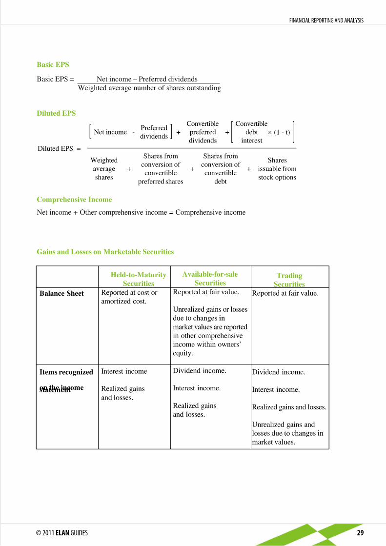
Basic EPS
Diluted EPS =
Weighted
average
shares
Shares from
conversion of
convertible
preferred shares
Shares from
conversion of
convertible
debt
Shares
issuable from
stock options
+ + +
Net incomePreferred
dividends
Convertible
preferred
dividends
Convertible
debt
interest
(1 - t)++-[ ] [ ]
Basic EPS = Net income – Preferred dividends
Weighted average number of shares outstanding
Net income + Other comprehensive income = Comprehensive income
Diluted EPS
Comprehensive Income
Balance Sheet
Items recognized
on the incomestatement
Held-to-Maturity
Securities
Reported at cost or
amortized cost.
Interest income
Realized gains
and losses.
Available-for-sale
Securities
Reported at fair value.
Unrealized gains or losses
due to changes in
market values are reported
in other comprehensive
income within owners’
equity.
Dividend income.
Interest income.
Realized gains
and losses.
Trading
Securities
Reported at fair value.
Dividend income.
Interest income.
Realized gains and losses.
Unrealized gains and
losses due to changes in
market values.
Gains and Losses on Marketable Securities
© 2011 ELAN GUIDES 29
FINANCIAL REPORTING AND ANALYSIS

5/13/2018 2012.CFA.L1.Formula.sheet (1) - slidepdf.com
http://slidepdf.com/reader/full/2012cfal1formulasheet-1 30/73
CFI
Inflows
Sale proceeds from fixed assets.
Sale proceeds from long-term investments.
CFF
Inflows
Proceeds from debt issuance.
Proceeds from issuance of equity instruments.
Outflows
Purchase of fixed assets.
Cash used to acquire LT investment
securities.
Outflows
Repayment of LT debt.
Payments made to repurchase stock.
Dividends payments.
CFO
Inflows
Cash collected from customers.Interest and dividends received.
Proceeds from sale of securities held for trading.
Outflows
Cash paid to employees.Cash paid to suppliers.
Cash paid for other expenses.
Cash used to purchase trading
securities.
Interest paid.
Taxes paid.
Classification of Cash Flows
Interest and dividends received
Interest paid
Dividend paid
Dividends received
Taxes paid
Bank overdrafts
Presentation Format
CFO
(No difference in CFI and
CFF presentation)
Disclosures
CFO or CFI
CFO or CFF
CFO or CFF
CFO or CFI
CFO, but part of the tax can be
categorized as CFI or CFF if it is clear
that the tax arose from investing or
financing activities.
Included as a part of cash equivalents.
Direct or indirect method. The former is
preferred.
Taxes paid should be presented separately
on the cash flow statement.
CFO
CFO
CFF
CFO
CFO
Not considered a part of cash equivalents
and included in CFF.
Direct or indirect method. The former is
preferred. However, if the direct method
is used, a reconciliation of net income
and CFO must be included.
If taxes and interest paid are not explicitly
stated on the cash flow statement, details
can be provided in footnotes.
IFRS U.S. GAAP
Cash Flow Statements under IFRS and U.S. GAAP
Cash Flow Classification under U.S. GAAP
© 2011 ELAN GUIDES 30
FINANCIAL REPORTING AND ANALYSIS

5/13/2018 2012.CFA.L1.Formula.sheet (1) - slidepdf.com
http://slidepdf.com/reader/full/2012cfal1formulasheet-1 31/73
Free Cash Flow to the Firm
FCFE = CFO - FCInv + Net borrowing
FCFF = NI + NCC + [Int * (1 – tax rate)] – FCInv – WCInv
FCFF = CFO + [Int * (1 – tax rate)] – FCInv
Free Cash Flow to Equity
Inventory turnover =
Cost of goods sold
Average inventory
Inventory Turnover
Days of inventory on hand (DOH) =
365
Inventory turnover
Days of Inventory on Hand
Receivables turnover =
Revenue
Average receivables
Receivables Turnover
Days of sales outstanding (DSO) =
365
Receivables turnover
Days of Sales Outstanding
Payables turnover =
Purchases
Average trade payables
Payables Turnover
Number of days of payables =
365
Payables turnover
Number of Days of Payables
Working capital turnover =
Revenue
Average working capital
Working Capital Turnover
Fixed asset turnover =
Revenue
Average fixed assets
Fixed Asset Turnover
Total Asset Turnover = RevenueAverage total assets
Total Asset Turnover
© 2011 ELAN GUIDES 31
FINANCIAL REPORTING AND ANALYSIS

5/13/2018 2012.CFA.L1.Formula.sheet (1) - slidepdf.com
http://slidepdf.com/reader/full/2012cfal1formulasheet-1 32/73
Current Ratio
Current ratio =
Current assets
Current liabilities
Quick ratio =
Cash + Short-term marketable investments + Receivables
Current liabilities
Quick Ratio
Cash ratio =
Cash + Short-term marketable investments
Current liabilities
Cash Ratio
Defensive interval ratio = Cash + Short-term marketable investments + ReceivablesDaily cash expenditures
Defensive Interval Ratio
Cash conversion cycle = DSO + DOH – Number of days of payables
Cash Conversion Cycle
Debt-to-assets ratio =
Total debt
Total assets
Debt-to-Assets Ratio
Debt-to-capital ratio =
Total debt
Total debt + Shareholders’ equity
Debt-to-Capital Ratio
Debt-to-equity ratio =
Total debt
Shareholders’ equity
Debt-to-Equity Ratio
Financial leverage ratio =
Average total assets
Average total equity
Financial Leverage Ratio
Interest coverage ratio =
EBIT
Interest payments
Interest Coverage Ratio
Fixed charge coverage ratio =
EBIT + Lease payments
Interest payments + Lease payments
Fixed Charge Coverage Ratio
Gross profit margin =
Gross profit
Revenue
Gross Profit Margin
© 2011 ELAN GUIDES 32
FINANCIAL REPORTING AND ANALYSIS

5/13/2018 2012.CFA.L1.Formula.sheet (1) - slidepdf.com
http://slidepdf.com/reader/full/2012cfal1formulasheet-1 33/73
Operating Profit Margin
Operating profit margin =
Operating profit
Revenue
Net profit margin =
Net profit
Revenue
Net Profit Margin
Pretax margin =
EBT (earnings before tax, but after interest)
Revenue
Pretax Margin
ROA = Net incomeAverage total assets
Adjusted ROA =
Net income + Interest expense (1 – Tax rate)
Average total assets
Operating ROA =
Operating income or EBIT
Average total assets
Return on Assets
Return on total capital =
EBIT
Short-term debt + Long-term debt + Equity
Return on Total Capital
Return on equity =
Net income
Average total equity
Return on Equity
Return on common equity =
Net income – Preferred dividends
Average common equity
Return on Common Equity
ROE = Net incomeAverage shareholders’ equity
DuPont Decomposition of ROE
2-Way Dupont Decomposition
ROE =Net income
Average total assets
Average total assets Average shareholder’s equity
ROA Leverage
3-Way Dupont Decomposition
ROE = Net income Revenue Average total assetsRevenue Average total assets Average shareholders’ equity
Net profit margin Asset turnover Leverage
© 2011 ELAN GUIDES 33
FINANCIAL REPORTING AND ANALYSIS

5/13/2018 2012.CFA.L1.Formula.sheet (1) - slidepdf.com
http://slidepdf.com/reader/full/2012cfal1formulasheet-1 34/73
P/CF =
Price per share
Cash flow per share
Price to Cash Flow
P/S =
Price per share
Sales per share
Price to Sales
P/BV =
Price per share
Book value per share
Price to Book Value
P/E =
Price per share
Earnings per share
Price- to-Earnings Ratio
Dividends per share = Common dividends declaredWeighted average number of ordinary shares
Cash flow per share =Cash flow from operations
Average number of shares outstanding
EBITDA per share =EBITDA
Average number of shares outstanding
Per Share Ratios
Dividend payout ratio =Common share dividends
Net income attributable to common shares
Dividend Payout Ratio
Retention Rate =Net income attributable to common shares – Common share dividends
Net income attributable to common shares
Retention Rate
Sustainable growth rate = Retention rate ROE
Growth Rate
5-Way Dupont Decomposition
ROE =Net income
EBT
EBIT
Revenue
Average total assets
EBT EBIT Revenue Average total assets Avg. shareholders’ equity
Tax burden
Interest burden
EBIT margin
Asset turnover
Leverage
© 2011 ELAN GUIDES 34
FINANCIAL REPORTING AND ANALYSIS

5/13/2018 2012.CFA.L1.Formula.sheet (1) - slidepdf.com
http://slidepdf.com/reader/full/2012cfal1formulasheet-1 35/73
LIFO versus FIFO (with rising prices and stable inventory levels.)
COGS
Income before taxes
Income taxes
Net income
Cash flow
EI
Working capital
LIFO
Higher
Lower
Lower
Lower
Higher
Lower
Lower
FIFO
Lower
Higher
Higher
Higher
Lower
Higher
Higher
LIFO versus FIFO when Prices are Rising
Effect on
Numerator
Income is lower
under LIFO because
COGS is higher
Same debt levels
Current assets are
lower under LIFO
because EI is lower.
Assets are higher as
a result of lower
taxes paid
COGS is higher
under LIFO
Sales are the same
Type of Ratio
Profitability ratios.
NP and GP margins
Debt to equity
Current ratio
Quick ratio
Inventory turnover
Total asset turnover
Effect on
Denominator
Sales are the same
under both.
Lower equity under
LIFO
Current liabilities
are the same.
Current liabilities
are the same
Average inventory
is lower under LIFO
Lower total assets
under LIFO
Effect on Ratio
Lower under LIFO.
Higher under LIFO
Lower under LIFO
Higher under LIFO
Higher under LIFO
Higher under LIFO
© 2011 ELAN GUIDES 35
FINANCIAL REPORTING AND ANALYSIS

5/13/2018 2012.CFA.L1.Formula.sheet (1) - slidepdf.com
http://slidepdf.com/reader/full/2012cfal1formulasheet-1 36/73
Net income decreases by the entire after-tax
amount of the cost.
No related asset is recorded on the balance
sheet and therefore, no depreciation oramortization expense is charged in future
periods.
Operating cash flow decreases.
Expensed costs have no financial statement
impact in future years.
Initially when the cost is
capitalized
In future periods when the asset
is depreciated or amortized
Effect on Financial Statements
Noncurrent assets increase.
Cash flow from investing activities decreases.
Noncurrent assets decrease.
Net income decreases.
Retained earnings decrease.
Equity decreases.
When the cost is expensed
Net income (first year)Net income (future years)
Total assets
Shareholders’ equity
Cash flow from operations
Cash flow from investing
Income variability
Debt to equity
Capitalizing
HigherLower
Higher
Higher
Higher
Lower
Lower
Lower
Expensing
LowerHigher
Lower
Lower
Lower
Higher
Higher
Higher
Financial Statement Effects of Capitalizing versus Expensing
© 2011 ELAN GUIDES 36
FINANCIAL REPORTING AND ANALYSIS

5/13/2018 2012.CFA.L1.Formula.sheet (1) - slidepdf.com
http://slidepdf.com/reader/full/2012cfal1formulasheet-1 37/73
Straight Line Depriciation
Depreciation expense =Original cost - Salvage value
Depreciable life
DDB depreciation in Year X =2
Book value at the beginning of Year XDepreciable life
Accelerated Depriciation
Estimated useful life = Gross investment in fixed assets
Annual depreciation expense
Estimated Useful Life
Average age of asset = Accumulated depreciationAnnual depreciation expense
Average Cost of Asset
Remaining useful life = Net investment in fixed assets
Annual depreciation expense
Remaining Useful Life
Carrying amount is greater.Tax base is greater.
Carrying amount is greater.
Tax base is greater.
Treatment of Temporary Differences
© 2011 ELAN GUIDES 37
FINANCIAL REPORTING AND ANALYSIS

5/13/2018 2012.CFA.L1.Formula.sheet (1) - slidepdf.com
http://slidepdf.com/reader/full/2012cfal1formulasheet-1 38/73
Income Tax Accounting under IFRS versus U.S. GAAP
Revaluation is prohibited.
No recognition of deferred
taxes for foreign subsidiaries
that fulfill indefinite reversal
criteria.
No recognition of deferred
taxes for domestic
subsidiaries when amountsare tax-free.
No recognition of deferred
taxes for foreign corporate
joint ventures that fulfill
indefinite reversal criteria.
Deferred taxes are recognized
from temporary differences.
Only enacted tax rates and
tax laws are used.
Deferred tax assets are
recognized in full and thenreduced by a valuation
allowance if it is likely that
they will not be realized.
Same as in IFRS.
Classified as either current ornoncurrent based on
classification of underlying
asset and liability.
Revaluation of fixed
assets and intangible
assets.
Treatment of
undistributed profit
from investment in
subsidiaries.
Treatment of
undistributed profit
from investments in
joint ventures.
Treatment of
undistributed profitfrom investments in
associates.
Tax rates.
Deferred tax asset
recognition.
Offsetting of deferred
tax assets and liabilities.
Balance sheetclassification.
Recognized in equity as deferred
taxes.
Recognized as deferred taxes
except when the parent company
is able to control the distribution
of profits and it is probable that
temporary differences will not
reverse in future.
Recognized as deferred taxes
except when the investor controls
the sharing of profits and it is
probable that there will be no
reversal of temporary differences
in future.
Recognized as deferred taxes
except when the investor controlsthe sharing of profits and it is
probable that there will be no
reversal of temporary differences
in future.
Tax rates and tax laws enacted
or substantively enacted.
Recognized if it is probable that
sufficient taxable profit will beavailable in the future.
Offsetting allowed only if the
entity has right to legally enforce
it and the balance is related to a
tax levied by the same authority.
Classified on balance sheet asnet noncurrent with
supplementary disclosures.
IFRS U.S. GAAP
ISSUE SPECIFIC TREATMENTS
DEFERRED TAX MEASUREMENT
DEFERRED TAX PRESENTATION
© 2011 ELAN GUIDES 38
FINANCIAL REPORTING AND ANALYSIS
5/13/2018 2012.CFA.L1.Formula.sheet (1) - slidepdf.com
http://slidepdf.com/reader/full/2012cfal1formulasheet-1 39/73
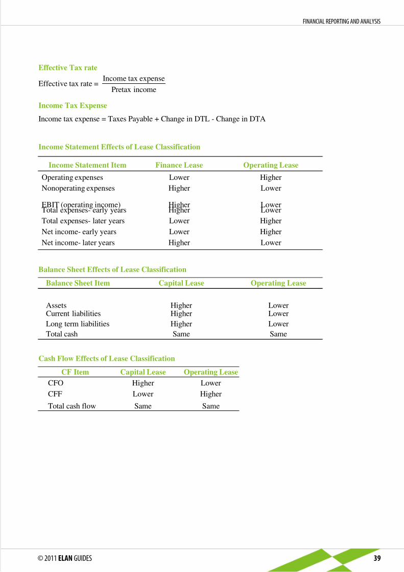
Effective Tax rate
Income tax expense
Pretax incomeEffective tax rate =
Income tax expense = Taxes Payable + Change in DTL - Change in DTA
Income Tax Expense
Income Statement Effects of Lease Classification
Income Statement Item
Operating expenses
Nonoperating expenses
EBIT (operating income)Total expenses- early years
Total expenses- later years
Net income- early years
Net income- later years
Finance Lease
Lower
Higher
HigherHigher
Lower
Lower
Higher
Operating Lease
Higher
Lower
LowerLower
Higher
Higher
Lower
Balance Sheet Item
AssetsCurrent liabilities
Long term liabilities
Total cash
Capital Lease
HigherHigher
Higher
Same
Operating Lease
LowerLower
Lower
Same
Balance Sheet Effects of Lease Classification
CF Item
CFO
CFF
Total cash flow
Capital Lease
Higher
Lower
Same
Operating Lease
Lower
Higher
Same
Cash Flow Effects of Lease Classification
© 2011 ELAN GUIDES 39
FINANCIAL REPORTING AND ANALYSIS

5/13/2018 2012.CFA.L1.Formula.sheet (1) - slidepdf.com
http://slidepdf.com/reader/full/2012cfal1formulasheet-1 40/73
Impact of Lease Classification on Financial Ratios
Effect on Ratio
Lower
Lower
Lower
Higher
Lower
Denominator
under FinanceLease
Assets- higher
Assets- higher
Current
liabilities-
higher
Equity same.
Assets higher
Equity same
Numerator
under FinanceLease
Sales- same
Net income lower
in early years
Current assets-
same
Debt- higher
Net income lower
in early years
Ratio Better or
Worse underFinance Lease
Worse
Worse
Worse
Worse
Worse
Ratio
Asset turnover
Return on assets*
Current ratio
Leverage ratios
(D/E and D/A)
Return on equity*
* In early years of the lease agreement.
Operating Lease
Same
Lower
Lower
Higher
Lower
Same
Financing Lease
Same
Higher
Higher
Lower
Higher
Same
Total net income
Net income (early years)
Taxes (early years)
Total CFO
Total CFI
Total cash flow
Financial Statement Effects of Lease Classification from Lessor’s Perspective
© 2011 ELAN GUIDES 40
FINANCIAL REPORTING AND ANALYSIS

5/13/2018 2012.CFA.L1.Formula.sheet (1) - slidepdf.com
http://slidepdf.com/reader/full/2012cfal1formulasheet-1 41/73
Solvency Ratios
Leverage Ratios
Debt-to-assets ratio
Debt-to-capital ratio
Debt-to-equity ratio
Financial leverage ratio
Coverage Ratios
Interest coverage ratio
Fixed charge coverage ratio
Numerator
Total debt
Total debt
Total debt
Average total assets
EBIT
EBIT + Lease
payments
Denominator
Total assets
Total debt + Total
shareholders’ equity
Total shareholders’
equity
Average shareholders’
equity
Interest payments
Interest payments +
Lease payments
Description
Expresses the percentage
of total assets financed by
debt
Measures the percentage
of a company’s total capital
(debt + equity) financed by
debt.
Measures the amount of
debt financing relative to
equity financing
Measures the amount of
total assets supported by
one money unit of equity.
Measures the number of times a company’s EBIT
could cover its interest
payments.
Measures the number of
times a company’s earnings
(before interest, taxes and
lease payments) can cover
the company’s interest and
lease payments.
Definitions of Commonly Used Solvency Ratios
© 2011 ELAN GUIDES 41
FINANCIAL REPORTING AND ANALYSIS

5/13/2018 2012.CFA.L1.Formula.sheet (1) - slidepdf.com
http://slidepdf.com/reader/full/2012cfal1formulasheet-1 42/73
Gross investment in fixed assets=
Accumulated depreciation+
Net investment in fixed assets
Annual depreciation expense Annual depreciation expense Annual depreciation expense
Estimated useful or depreciable
life
The historical cost of an asset
divided by its useful life equals
annual depreciation expense under
the straight line method. Therefore,
the historical cost divided by annual
depreciation expense equals the
estimated useful life.
Average age of asset
Annual depreciation expense times
the number of years that the asset
has been in use equals
accumulated depreciation.
Therefore, accumulated
depreciation divided by annual
depreciation equals the average
age of the asset.
Remaining useful life
The book value of the asset divided
by annual depreciation expense
equals the number of years the asset
has remaining in its useful life.
Adjustments related to inventory:
EIFIFO = EILIFO + LR
whereLR = LIFO Reserve
COGSFIFO = COGSLIFO - (Change in LR during the year)
Net income after tax under FIFO will be greater than LIFO net income after tax by:
Change in LIFO Reserve (1 - Tax rate)
When converting from LIFO to FIFO assuming rising prices:
Equity (retained earnings) increase by:
LIFO Reserve (1 - Tax rate)
Liabilities (deferred taxes) increase by:
LIFO Reserve (Tax rate)
Current assets (inventory) increase by:
LIFO Reserve
Adjustments related to property, plant and equipment:
© 2011 ELAN GUIDES 42
FINANCIAL REPORTING AND ANALYSIS

5/13/2018 2012.CFA.L1.Formula.sheet (1) - slidepdf.com
http://slidepdf.com/reader/full/2012cfal1formulasheet-1 43/73
Categories of Marketable Securities and Accounting Treatment
Classification
Balance Sheet
Value
Unrealized and
Realized Gains and
Losses
Income (Interest &
Dividends)
Held-to-maturity Amortized cost
(Par value +/-
unamortized
premium/ discount).
Unrealized: Not
reported
Realized:
Recognized on
income statement.
Recognized on
income statement.
Held-for-trading
Available-for-sale
Fair Value. Unrealized:
Recognized on
income statement.
Realized:
Recognized on
income statement.
Unrealized:
Recognized in other
comprehensive
income.
Realized:
Recognized on
income statement.
Recognized on
income statement.
Recognized on
income statement.Fair Value.
© 2011 ELAN GUIDES 43
FINANCIAL REPORTING AND ANALYSIS

5/13/2018 2012.CFA.L1.Formula.sheet (1) - slidepdf.com
http://slidepdf.com/reader/full/2012cfal1formulasheet-1 44/73
Inventory Accounting under IFRS versus U.S. GAAP
Property, Plant and Equipment
The increase in the asset’s
value from revaluation is
reported as a part of equity
unless it is reversing a
previously-recognized
decrease in the value of the
asset.
A decrease in the value of
the asset is reported on the
income statement unless it
is reversing a previously-
reported upward
revaluation.
U.S. GAAP
IFRS
Balance Sheet
Cost minus
accumulated
depreciation.
Cost minus
accumulated
depreciation.
Effects of Changes
in Balance Sheet
Value
Changes in Balance
Sheet Value
Does not permit upward
revaluation.No effect.
Permits upward
revaluation.
Asset is reported at fair
value at the revaluation
date less accumulated
depreciation following
the revaluation.
Permitted Cost
Recognition MethodsChanges in Balance
Sheet Value
U.S. GAAP
IFRS
Balance Sheet
Lower of cost or
market.
Lower of cost or net
realizable value.
FIFO.
Weighted Average
Cost.
Permits inventory
write downs,
and also reversals of
write downs.
LIFO.
FIFO.
Weighted average
cost.
Permits inventory
write downs,
but not reversal of
write downs.
© 2011 ELAN GUIDES 44
FINANCIAL REPORTING AND ANALYSIS

5/13/2018 2012.CFA.L1.Formula.sheet (1) - slidepdf.com
http://slidepdf.com/reader/full/2012cfal1formulasheet-1 45/73
Percent Ownership Extent of Control Accounting Treatment
Less than 20% No significant control Classified as held-to-maturity, trading,or available for sale securities.
20% - 50% Significant Influence
Significant Control
Equity method.
Consolidation.
Shared (joint ventures)
More than 50%
Joint Control Equity method/ proportionate
consolidation.
Long-Term Investments
U.S. GAAP
IFRS
Balance Sheet
Only purchased intangibles
may be recognized as
assets. Internally developed
items cannot be recognized
as assets.
Reported at cost minus
accumulated amortization
for assets with finite useful
lives.
Reported at cost minus
impairment for assets with
infinite useful lives.
Only purchased intangibles
may be recognized as
assets. Internally developed
items cannot be recognized
as assets.
Reported at cost minus
accumulated amortization
for assets with finite useful
lives.
Reported at cost minus
impairment for assets with
infinite useful lives.
Effects of Changes in
Balance Sheet
Value
No effect.
An increase in value is
recognized as a part of
equity unless it is a
reversal of a
previously recognized
downward revaluation.
A decrease in value is
recognized on the
income statement
unless it is a reversalof a previously
recognized upward
revaluation.
Changes in
Balance Sheet
Value
Does not permit
upward
revaluation.
Permits upward
revaluation.
Assets are
reported at fair
value as of the
revaluation date
less subsequent
accumulated
amortization.
Treatment of Identifiable Intangible Assets
© 2011 ELAN GUIDES 45
FINANCIAL REPORTING AND ANALYSIS

5/13/2018 2012.CFA.L1.Formula.sheet (1) - slidepdf.com
http://slidepdf.com/reader/full/2012cfal1formulasheet-1 46/73
Long-Term Contracts
U.S. GAAP
IFRS
Outcome can be reliably
estimated
Percentage-of-completion
method.
Percentage-of-completion
method.
Outcome cannot be reliably
estimated
Completed contract
method.
Revenue is recognized to the
extent that it is probable to
recover contract costs.
Profit is only recognized at project
completion.
© 2011 ELAN GUIDES 46
FINANCIAL REPORTING AND ANALYSIS

5/13/2018 2012.CFA.L1.Formula.sheet (1) - slidepdf.com
http://slidepdf.com/reader/full/2012cfal1formulasheet-1 47/73
CORPORATE FINANCE
where
CFt = after-tax cash flow at time, t.
r = required rate of return for the investment. This is the firm’s cost of capital adjusted
for the risk inherent in the project.
Outlay = investment cash outflow at t = 0.
AAR =Average net income
Average book value
PI = PV of future cash flows = 1 + NPVInitial investment Initial investment
Where:
wd = Proportion of debt that the company uses when it raises new funds
rd = Before-tax marginal cost of debt
t = Company’s marginal tax ratewp = Proportion of preferred stock that the company uses when it raises new funds
rp = Marginal cost of preferred stock
we = Proportion of equity that the company uses when it raises new funds
re = Marginal cost of equity
Net Present Value (NPV)
Internal Rate of Return (IRR)
Average Accounting Rate of Return (AAR)
Profitability Index
Weighted Average Cost of Capital
To Transform Debt-to-equity Ratio into a component’s weight
© 2011 ELAN GUIDES 47
CORPORATE FINANCE

5/13/2018 2012.CFA.L1.Formula.sheet (1) - slidepdf.com
http://slidepdf.com/reader/full/2012cfal1formulasheet-1 48/73
where:
P0 = current market price of the bond.
PMTt = interest payment in period t.
rd = yield to maturity on BEY basis.
n = number of periods remaining to maturity.
FV = Par or maturity value of the bond.
Vp =Dp
rp
where:
Vp = current value (price) of preferred stock..
Dp = preferred stock dividend per share.
rp = cost of preferred stock.
Valuation of Bonds
Valuation of Preferred Stock
where
[E(RM) - RF] = Equity risk premium.
RM = Expected return on the market.
i = Beta of stock . Beta measures the sensitivity of the stock’s returns to
changes in market returns.
RF = Risk-free rate.
re = Expected return on stock (cost of equity)
re = RF + i[E(RM) - RF]
Capital Asset Pricing Model
where:
P0 = current market value of the security.
D1= next year’s dividend.
re = required rate of return on common equity.g = the firm’s expected constant growth rate of dividends.
Dividend Discount Model
Required Return on a Stock
© 2011 ELAN GUIDES 48
CORPORATE FINANCE

5/13/2018 2012.CFA.L1.Formula.sheet (1) - slidepdf.com
http://slidepdf.com/reader/full/2012cfal1formulasheet-1 49/73
Where (1 - (D/EPS)) = Earnings retention rate
Sustainable Growth Rate
r
Country risk
premium
Sovereign yield
spread=
Annualized standard deviation of equity index
Annualized standard deviation of sovereign
bond market in terms of the developed market
currency
Break point =Amount of capital at which a component’s cost of capital changes
Proportion of new capital raised from the component
Country Risk Premium
Bond Yield plus Risk Premium Approach
DOL =Percentage change in operating income
Percentage change in units sold
Degree of Operating Leverage
Rearranging the above equation gives us a formula to calculate the required return on equity:
To Unlever the beta
To Lever the beta
© 2011 ELAN GUIDES 49
CORPORATE FINANCE

5/13/2018 2012.CFA.L1.Formula.sheet (1) - slidepdf.com
http://slidepdf.com/reader/full/2012cfal1formulasheet-1 50/73
DOL =Q (P – V)
Q (P – V) – F
where:Q = Number of units sold
P = Price per unit
V = Variable operating cost per unit
F = Fixed operating cost
Q (P – V) = Contribution margin (the amount that units sold contribute to covering fixed
costs)
(P – V) = Contribution margin per unit
Degree of Financial Leverage
DFL =Percentage change in net income
Percentage change in operating income
DFL = =[Q(P – V) – F](1 – t)
[Q(P – V) – F – C](1 – t)
[Q(P – V) – F]
[Q(P – V) – F – C]
where:
Q = Number of units soldP = Price per unit
V = Variable operating cost per unit
F = Fixed operating cost
C = Fixed financial cost
t = Tax rate
Degree of Total Leverage
DTL =Percentage change in net income
Percentage change in the number of units sold
DTL = DOL DFL
DTL =Q (P – V)
[Q(P – V) – F – C]
where:
Q = Number of units produced and sold
P = Price per unitV = Variable operating cost per unit
F = Fixed operating cost
C = Fixed financial cost
© 2011 ELAN GUIDES 50
CORPORATE FINANCE

5/13/2018 2012.CFA.L1.Formula.sheet (1) - slidepdf.com
http://slidepdf.com/reader/full/2012cfal1formulasheet-1 51/73
PQ = VQ + F + C
where:
P = Price per unit
Q = Number of units produced and sold
V = Variable cost per unit
F = Fixed operating costs
C = Fixed financial cost
The breakeven number of units can be calculated as:
QBE
=F + C
P – V
Operating breakeven point
PQOBE = PV + F
QOBE =F
P – V
Break point
© 2011 ELAN GUIDES 51
CORPORATE FINANCE

5/13/2018 2012.CFA.L1.Formula.sheet (1) - slidepdf.com
http://slidepdf.com/reader/full/2012cfal1formulasheet-1 52/73
’
Purchases = Ending inventory + COGS - Beginning inventory
© 2011 ELAN GUIDES 52
CORPORATE FINANCE

5/13/2018 2012.CFA.L1.Formula.sheet (1) - slidepdf.com
http://slidepdf.com/reader/full/2012cfal1formulasheet-1 53/73
% Discount =Face value - Price
Price
365
Inventory turnover
Number of days of payables =Accounts payable
Average day’s purchases
Accounts payable
Purchases / 365
365
Payables turnover=
© 2011 ELAN GUIDES 53
CORPORATE FINANCE

5/13/2018 2012.CFA.L1.Formula.sheet (1) - slidepdf.com
http://slidepdf.com/reader/full/2012cfal1formulasheet-1 54/73
© 2011 ELAN GUIDES 54
CORPORATE FINANCE

5/13/2018 2012.CFA.L1.Formula.sheet (1) - slidepdf.com
http://slidepdf.com/reader/full/2012cfal1formulasheet-1 55/73
Holding Period Return
PT + DT
P0
- 1=
R =Pt – Pt-1 + Dt
Pt-1
+Pt – Pt-1
Pt-1
Dt
Pt-1
= Capital gain + Dividend yield=
where:
Pt = Price at the end of the period
Pt-1 = Price at the beginning of the period
Dt = Dividend for the period
Holding Period Returns for more than One Period
R = [(1 + R1) (1 + R2) .... (1 + Rn)] – 1
where:
R1, R2,..., Rn are sub-period returns
Geometric Mean Return
R = {[(1 + R1) (1 + R2) .... (1 + Rn)]1/n
} – 1
Annualized Return
rannual = (1 + rperiod)n- 1
where:
r = Return on investment
n = Number of periods in a year
PORTFOLIO MANAGEMENT
© 2011 ELAN GUIDES 55
PORTFOLIO MANAGEMENT

5/13/2018 2012.CFA.L1.Formula.sheet (1) - slidepdf.com
http://slidepdf.com/reader/full/2012cfal1formulasheet-1 56/73
Portfolio Return
Rp = w1R1 + w2R2
where:Rp = Portfolio return
w1 = Weight of Asset 1
w2 = Weight of Asset 2
R1 = Return of Asset 1
R2 = Return of Asset 2
Variance of a Single Asset
2
=
(Rt - )2
T
T
t = 1
where:
Rt = Return for the period t
T = Total number of periods
= Mean of T returns
Variance of a Representative Sample of the Population
s2
=
(Rt - R)2
T-1
T
t = 1
where:
R = mean return of the sample observations
s2
= sample variance
Standard Deviation of an Asset
=
(Rt - )2
T
T
t = 1s =
(Rt - R)2
T-1
T
t = 1
Variance of a Portfolio of Assets
P =2 wiw jCov(Ri,R j)
N
i,j = 1, i j
N
i = 1
wi Var(Ri) +2
P =2 wiw jCov(Ri,R j)N
i,j = 1
© 2011 ELAN GUIDES 56
PORTFOLIO MANAGEMENT

5/13/2018 2012.CFA.L1.Formula.sheet (1) - slidepdf.com
http://slidepdf.com/reader/full/2012cfal1formulasheet-1 57/73
Standard Deviation of a Portfolio of Two Risky Assets
U = E(R) A2
2
Utility Function
where:
U = Utility of an investment
E(R) = Expected return2
= Variance of returns
A = Additional return required by the investor to accept an additional unit of risk.
The CAL has an intercept of RFR and a constant slope that equals:
Capital Allocation Line
Expected Return on portfolios that lie on CML
E(Rp) = w1Rf + (1 - w1) E(Rm)
Variance of portfolios that lie on CML
2
= w1 f + (1 - w1) m + 2w1(1 - w1)Cov(Rf ,Rm)2 2 2 2
Equation of CML
E(Rp) = Rf + p
E(Rm) - Rf
m
where:
y-intercept = Rf = risk-free rate
slope = = market price of risk.E(Rm) - Rf
m
© 2011 ELAN GUIDES 57
PORTFOLIO MANAGEMENT

5/13/2018 2012.CFA.L1.Formula.sheet (1) - slidepdf.com
http://slidepdf.com/reader/full/2012cfal1formulasheet-1 58/73
Total Risk = Systematic risk + Unsystematic risk
Systematic and Nonsystematic Risk
Return-Generating Models
E(Ri) - Rf = k
j = 1
ij E(F j) =
i1[E(Rm) - Rf ] + ij E(F j)
k
j = 2
The Market Model
Ri = i + iRm + ei
Calculation of Beta
i =Cov(Ri,Rm)
m2
= =i,mim
m2
i,mi
m
The Capital Asset Pricing Model
E(Ri) = Rf + i[E(Rm) Rf ]
Sharpe ratio
Rp Rf
p
Sharpe ratio =
Treynor ratio
Rp Rf
p
Treynor ratio =
M-squared (M2)
m
p
M2
= (Rp Rf ) Rm Rf
Jensen’s alpha
pRp [Rf pRm Rf )]
Security Characteristic Line
Ri Rf iiRm Rf )
© 2011 ELAN GUIDES 58
PORTFOLIO MANAGEMENT

5/13/2018 2012.CFA.L1.Formula.sheet (1) - slidepdf.com
http://slidepdf.com/reader/full/2012cfal1formulasheet-1 59/73
The price at which an investor who goes long on a stock receives a margin call is calculated
as:
P0
(1 - Initial margin)
(1 – Maintenance margin)
The value of a price return index is calculated as follows:
VPRI =
ni Pi
D
N
i = 1
where:VPRI = Value of the price return index
ni = Number of units of constituent security i held in the index portfolio
N = Number of constituent securities in the index
Pi = Unit price of constituent security i
D = Value of the divisor
Price Return
PRI =VPRI1 VPRI0
VPRI0
where:
PRI = Price return of the index portfolio (as a decimal number)
VPRI1 = Value of the price return index at the end of the period
VPRI0 = Value of the price return index at the beginning of the period
The price return of an index can be calculated as:
The price return of each constituent security is calculated as:
PRi =Pi1 Pi0
Pi0
where:
PRi = Price return of constituent security i (as a decimal number)
Pi1 = Price of the constituent security i at the end of the period
Pi0 = Price of the constituent security i at the beginning of the period
EQUITY
© 2011 ELAN GUIDES 59
EQUITY

5/13/2018 2012.CFA.L1.Formula.sheet (1) - slidepdf.com
http://slidepdf.com/reader/full/2012cfal1formulasheet-1 60/73
The price return of the index equals the weighted average price return of the constituent
securities. It is calculated as:
PRI = w1PR1 + w2PR2 + ....+ wNPRN
where:
PRI = Price return of the index portfolio (as a decimal number)
PRi = Price return of constituent security i (as a decimal number)
wi = Weight of security i in the index portfolio
N = Number of securities in the index
Total Return
The total return of an index can be calculated as:
TRI =VPRI1 VPRI0 IncI
VPRI0
where:
TRI = Total return of the index portfolio (as a decimal number)
VPRI1 = Value of the total return index at the end of the period
VPRI0 = Value of the total return index at the beginning of the period
IncI = Total income from all securities in the index held over the period
The total return of each constituent security is calculated as:
TRi =P1i P0i Inci
P0i
where:
TRi = Total return of constituent security i (as a decimal number)
P1i = Price of constituent security i at the end of the period
P0i = Price of constituent security i at the beginning of the period
Inci = Total income from security i over the period
The total return of the index equals the weighted average total return of the constituent
securities. It is calculated as:
TRI = w1TR1 + w2TR2 + ....+ wNTRN
where:
TRI = Total return of the index portfolio (as a decimal number)
TRi = Total return of constituent security i (as a decimal number)
wi = Weight of security i in the index portfolio
N = Number of securities in the index
© 2011 ELAN GUIDES 60
EQUITY

5/13/2018 2012.CFA.L1.Formula.sheet (1) - slidepdf.com
http://slidepdf.com/reader/full/2012cfal1formulasheet-1 61/73
Calculation of Index Returns over Multiple Time Periods
Given a series of price returns for an index, the value of a price return index can be calculated
as:
VPRIT = VPRI0 (1 + PRI1) (1 + PRI2) ... (1 + PRIT)
where:
VPRI0 = Value of the price return index at inception
VPRIT = Value of the price return index at time t
PRIT = Price return (as a decimal number) on the index over the period
VTRIT = VTRI0 (1 + TRI1) (1 + TRI2) ... (1 + TRIT)
Similarly, the value of a total return index may be calculated as:
where:
VTRI0 = Value of the index at inception
VTRIT = Value of the index at time t
TRIT = Total return (as a decimal number) on the index over the period
Price Weighting
wi =P
Pi
N
i = 1
Pi
Equal Weighting
wi =E
N
1
where:
wi = Fraction of the portfolio that is allocated to security i or weight of security i
N = Number of securities in the index
Market-Capitalization Weighting
wi =M
Q jP jN
j = 1
QiPi
where:
wi = Fraction of the portfolio that is allocated to security i or weight of security i
Qi = Number of shares outstanding of security iPi = Share price of security i
N = Number of securities in the index
© 2011 ELAN GUIDES 61
EQUITY

5/13/2018 2012.CFA.L1.Formula.sheet (1) - slidepdf.com
http://slidepdf.com/reader/full/2012cfal1formulasheet-1 62/73
The float-adjusted market-capitalization weight of each constituent security is calculated as:
wi =M
f jQ jP jN
j = 1
f iQiPi
where:
f i = Fraction of shares outstanding in the market float
wi = Fraction of the portfolio that is allocated to security i or weight of security i
Qi = Number of shares outstanding of security i
Pi = Share price of security i
N = Number of securities in the index
Fundamental Weighting
wi =F
F jN
j = 1
Fi
where:
Fi = A given fundamental size measure of company i
Return Characteristics of Equity Securities
Total Return, Rt = (Pt – Pt-1 + Dt) / Pt-1
where:
Pt-1 = Purchase price at time t – 1
Pt = Selling price at time t
Dt = Dividends paid by the company during the period
Accounting Return on Equity
ROEt = =NIt
Average BVEt
NIt
(BVEt + BVEt-1)/2
Dividend Discount Model (DDM)
© 2011 ELAN GUIDES 62
EQUITY

5/13/2018 2012.CFA.L1.Formula.sheet (1) - slidepdf.com
http://slidepdf.com/reader/full/2012cfal1formulasheet-1 63/73
One year holding period:
Multiple-Year Holding Period DDM
where:
Pn = Price at the end of n years.
Infinite Period DDM (Gordon Growth Model)
PV0 =D0 (1 + g
c)
1
(1 + k e)
1 +D0 (1 + g
c)
2
(1 + k e)
2 +D0 (1 + g
c)
3
(1 + k e)
3 +...+D0 (1 + g
c)
(1 + k e)
This equation simplifies to:
D0 (1 + gc)
1
(k e
- gc)
1PV = =D1
k e
- gc
The long-term (constant) growth rate is usually calculated as:
gc = RR ROE
Multi-Stage Dividend Discount Model
Dn = Last dividend of the supernormal growth period
Dn+1 = First dividend of the constant growth period
where:
The Free-Cash-Flow-to-Equity (FCFE) Model
FCFE = CFO – FC Inv + Net borrowing
© 2011 ELAN GUIDES 63
EQUITY

5/13/2018 2012.CFA.L1.Formula.sheet (1) - slidepdf.com
http://slidepdf.com/reader/full/2012cfal1formulasheet-1 64/73
Analysts may calculate the intrinsic value of the company’s stock by discounting their
projections of future FCFE at the required rate of return on equity.
V0 =
t = 1
FCFEt
(1 + k e)t
Value of a Preferred Stock
V0 =D0
r
When preferred stock is non-callable, non-convertible, has no maturity date and pays dividends
at a fixed rate, the value of the preferred stock can be calculated using the perpetuity formula:
For a non-callable, non-convertible preferred stock with maturity at time, n, the value of the
stock can be calculated using the following formula:
V0 = n
t = 1
Dt
(1 + r)t
F
(1 + r)n
+
where:
V0 = value of preferred stock today (t = 0)
Dt = expected dividend in year t, assumed to be paid at the end of the year
r = required rate of return on the stock F = par value of preferred stock
Price Multiples
=D1 /E1
r - g
P0
E1
Market price of share
Cash flow per share
Price to cash flow ratio =
Market price per share
Net sales per sharePrice to sales ratio =
Market value of equity
Total net salesPrice to sales ratio =
© 2011 ELAN GUIDES 64
EQUITY

5/13/2018 2012.CFA.L1.Formula.sheet (1) - slidepdf.com
http://slidepdf.com/reader/full/2012cfal1formulasheet-1 65/73
Current market price of share
Book value per shareP/BV =
Market value of common shareholders’ equity
Book value of common shareholders’ equityP/BV =
where:
Book value of common shareholders’ equity =
(Total assets - Total liabilities) - Preferred stock
Enterprise Value Multiples
EV/EBITDA
where:
EV = Enterprise value and is calculated as the market value of the company’s common stock
plus the market value of outstanding preferred stock if any, plus the market value of debt,
less cash and short term investments (cash equivalents).
© 2011 ELAN GUIDES 65
EQUITY

5/13/2018 2012.CFA.L1.Formula.sheet (1) - slidepdf.com
http://slidepdf.com/reader/full/2012cfal1formulasheet-1 66/73
FIXED INCOME
Coupon rate = K – L (Reference rate)
Bond Coupon
Coupon = Coupon rate Par value
Coupon Rate = Reference rate + Quoted margin
Coupon Rate (Floating)
Coupon Rate (Inverse Floaters)
Price of a callable bond = Value of option-free bond – Value of embedded call option
Callable Bond Price
Price of a putable bond = Value of option-free bond + Value of embedded put option
Putable Bond Price
Dollar duration = Duration Bond value
Dollar Duration
Nominal spread (Bond Y as the reference bond) = Yield on Bond X – Yield on Bond Y
Nominal spread
Relative yield spread =Yield on Bond X – Yield on Bond Y
Yield on Bond Y
Relative Yield spread
Yield ratio =
Yield on Bond X
Yield on Bond Y
Yield Ratio
After-tax yield = Pretax yield (1- marginal tax rate)
After-Tax Yield
Taxable-equivalent yield = Tax-exempt yield(1 – marginal tax rate)
Taxable-Equalent Yield
Inflation-Indexed Treasury Securities
TIPS coupon = Inflation adjusted par value (Stated coupon rate/2)
© 2011 ELAN GUIDES 66
FIXED INCOME

5/13/2018 2012.CFA.L1.Formula.sheet (1) - slidepdf.com
http://slidepdf.com/reader/full/2012cfal1formulasheet-1 67/73
Formula to Convert BEY into Annual-Pay YTM:
](Annual-pay yield = 1 +Yield on bond equivalent basis
2 -1
2
Bond Value =Maturity value
(1+i) years till maturity 2
where i equals the semiannual discount rate
Bond Value
Current yield =Annual cash coupon
Bond price
Current Yield
where:
Bond price = Full price including accrued interest.
CPNt = The semiannual coupon payment received after t semiannual periods.
N = Number of years to maturity.
YTM = Yield to maturity.
Bond price
Bond Price
BEY = [(1 + monthly CFY)6 – 1] 2
Formula to Convert Monthly Cash Flow Yield into BEY
d = (1-p)360
N
Discount Basis Yeild
Valuing a Bond Between Coupon Payments.
w =Days between settlement date and next coupon payment date
Days in coupon period
where:
w = Fractional period between the settlement date and the next coupon payment date.
Present value t =Expected cash flow
(1 + i) t – 1 + w
© 2011 ELAN GUIDES 67
FIXED INCOME

5/13/2018 2012.CFA.L1.Formula.sheet (1) - slidepdf.com
http://slidepdf.com/reader/full/2012cfal1formulasheet-1 68/73
Duration
Duration =V- - V+
2(V0)(y)
where:
y = change in yield in decimalV0 = initial priceV- = price if yields decline by yV+ = price if yields increase by y
Z-spread = OAS + Option cost; and OAS = Z-spread - Option cost
Z-Spread
Portfolio duration = w1D1 + w2D2 + …..+ wNDN
where:
N = Number of bonds in portfolio.
Di = Duration of Bond i.
wi = Market value of Bond i divided by the market value of portfolio.
Portfolio Duration
Percentage change in bond price = duration effect + convexity adjustment= {[-duration (y)] + [convexity (y)2]} 100where:
y = Change in yields in decimals.
Percentage Change in Bond Price
C =V+ + V- - 2V0
2V0(y)2
Convexity
Price value of a basis point = Duration 0.0001 bond value
Price Value of a Basis Point
© 2011 ELAN GUIDES 68
FIXED INCOME

5/13/2018 2012.CFA.L1.Formula.sheet (1) - slidepdf.com
http://slidepdf.com/reader/full/2012cfal1formulasheet-1 69/73
Floating rate at expiration – FRA rate (days in floating rate/ 360)
1 + [Floating rate at expiration (days in floating rate/ 360)
Numerator: Interest savings on the hypothetical loan. This number is positive when the floating rate
is greater than the forward rate. When this is the case, the long benefits and expects to receive a payment
from the short. The numerator is negative when the floating rate is lower than the forward rate. When this
is the case, the short benefits and expects to receive a payment from the long.
Denominator: The discount factor for calculating the present value of the interest savings.
FRA Payoff
DERIVATIVES
© 2011 ELAN GUIDES 69
DERIVATIVES

5/13/2018 2012.CFA.L1.Formula.sheet (1) - slidepdf.com
http://slidepdf.com/reader/full/2012cfal1formulasheet-1 70/73
Moneyness and Intrinsic Value of a Put Option
Call Option Payoffs
Put Option Payoffs
Intrinsic value of call = Max [0, (St - X)]
Intrinsic Value of a Call Option
© 2011 ELAN GUIDES 70
DERIVATIVES

5/13/2018 2012.CFA.L1.Formula.sheet (1) - slidepdf.com
http://slidepdf.com/reader/full/2012cfal1formulasheet-1 71/73
Strategy
fiduciary
call
long
call
long
put
long
underlying
asset
longbond
Consisting of
long call +
long bond
long
call
long
put
long
underlying
asset
longbond
Equals
=
=
=
=
=
Strategy
Protective
put
Synthetic
call
Synthetic put
Synthetic
underlying
asset
Syntheticbond
Consisting of
long put + long
underlying asset
long put + long
underlying asset+ short bond
long call + short
underlying asset
+ long bond
long call
+ long bond
+ short put
long put + longunderlying asset
+ short call
Value
P0 + S0
P0 + S0
- X/(1+RF)T
C0 - S0
+X/(1+RF)T
C0
+ X/(1+RF)T
- P0
P0 + S0
- C0
Synthetic Derivative Securities
Value
C0 + X
(1 + RF)T
C0
P0
S0
X(1 + RF)
T
Option
European call
American call
European put
American put
Minimum Value
ECt 0
ACt 0
EPt 0
APt 0
Maximum Value
ECt St
ACt St
EPt X/ (1 + RFR)T
APt X
Option Value Limits
Option premium = Intrinsic value + Time value
Option Premium
C0 + X = P0 + S0
(1 + RF)T
Put-Call Parity
© 2011 ELAN GUIDES 71
DERIVATIVES

5/13/2018 2012.CFA.L1.Formula.sheet (1) - slidepdf.com
http://slidepdf.com/reader/full/2012cfal1formulasheet-1 72/73
Option Value Bounds
Interest Rate Put Holder’s Payoff
= Max (0, Exercise rate – Underlying rate at expiration) (Days in underlying rate) NP
360
where:
NP = Notional principal
Interest Rate Call Holder’s Payoff
= Max (0, Underlying rate at expiration - Exercise rate) (Days in underlying Rate) NP
360
where: NP = Notional principal
Net fixed-rate paymentt = (Swap fixed rate - LIBORt-1 )(No. of days/360)(NP)
where:
NP equals the notional principal.
Net Payment for a Fixed-Rate-Payer
© 2011 ELAN GUIDES 72
DERIVATIVES
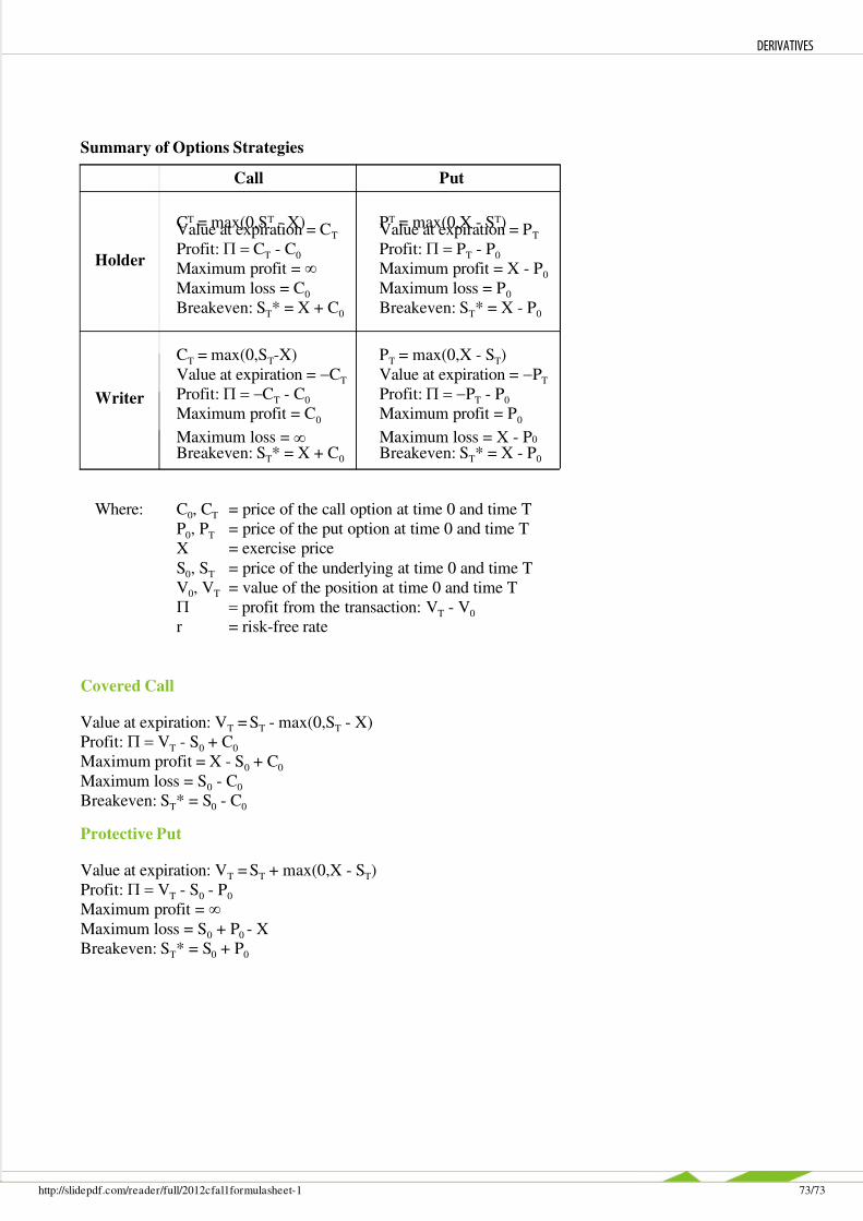
5/13/2018 2012.CFA.L1.Formula.sheet (1) - slidepdf.com
http://slidepdf.com/reader/full/2012cfal1formulasheet-1 73/73
C0, CT = price of the call option at time 0 and time T
P0, PT = price of the put option at time 0 and time T
X = exercise price
S0, ST = price of the underlying at time 0 and time T
V0, VT = value of the position at time 0 and time T
profit from the transaction: VT - V0
r = risk-free rate
CT = max(0,ST - X)Value at expiration = CT
Profit: CT - C0
Maximum profit = Maximum loss = C0
Breakeven: ST* = X + C0
PT = max(0,X - ST)Value at expiration = PT
Profit: PT - P0
Maximum profit = X - P0
Maximum loss = P0
Breakeven: ST* = X - P0
PT = max(0,X - ST)
Value at expiration = PT
Profit: PT - P0
Maximum profit = P0
Maximum loss = X - P0
Breakeven: ST* = X - P0
Call Put
Holder
Writer
CT = max(0,ST-X)
Value at expiration = CT
Profit: CT - C0
Maximum profit = C0
Maximum loss = Breakeven: ST* = X + C0
Summary of Options Strategies
Where:
Covered Call
Value at expiration: VT = ST - max(0,ST - X)
Profit: VT - S0 + C0
Maximum profit = X - S0 + C0
Maximum loss = S0 - C0
Breakeven: ST* = S0 - C0
Protective Put
Value at expiration: VT = ST + max(0,X - ST)
Profit: VT - S0 - P0
Maximum profit = Maximum loss = S0 + P0 - X
Breakeven: ST* = S0 + P0
DERIVATIVES


![Pomalidomide Activity Blood 2012 Dispenzieri Blood 2012-02-413161[1][1]](https://img.pdfslide.us/doc/110x75/577d1d8f1a28ab4e1e8c86af/pomalidomide-activity-blood-2012-dispenzieri-blood-2012-02-41316111.jpg)