2011/2012 upgraded cost model final version - · PDF file · 2014-12-02Report for the Danish Business Authority (DBA) 2011/2012 upgraded cost model – final version Reconciliation

Report for the Danish Business Authority (DBA)

2011/2012 upgraded cost model –

final version

Reconciliation paper for the calculation of

actual operator costs

17 July 2012

Ref: 19176-144

.

Ref: 19176-144 .

Contents

1 Introduction 3

2 Model calibration 5

3 Model reconciliation 7

3.1 Unit capital costs of equipment 9

3.2 Asset price trends 10

3.3 Asset lifetimes 11

3.4 Top-down capex 12

3.5 Top-down opex 13

4 Cost optimisation 14

5 Updates to calibration and reconciliation of the cost model 16

5.1 Updates related to calibration in the 5.0vD model 16

5.2 Updates related to reconciliation in the 5.0vD model 17

5.3 Updates to the 5.0vR model 19

2011/2012 upgraded cost model – final version

Ref: 19176-144 .

Copyright © 2012. Analysys Mason Limited has produced the information contained herein

for the Danish Business Authority (DBA). The ownership, use and disclosure of this

information are subject to the Commercial Terms contained in the contract between

Analysys Mason Limited and the DBA.

Analysys Mason Limited

St Giles Court

24 Castle Street

Cambridge CB3 0AJ

UK

Tel: +44 (0)845 600 5244

Fax: +44 (0)1223 460866

[email protected]

www.analysysmason.com

Registered in England No. 5177472

2011/2012 upgraded cost model – final version | 3

Ref: 19176-144 .

1 Introduction

In early 2011 the Danish Business Authority (DBA) contracted Analysys Mason Limited („Analysys

Mason‟) to undertake a significant upgrade of the original mobile long-run average incremental cost

(LRAIC) model (hereinafter referred to as „the original mobile LRAIC model‟ or „the v4 model)

used by the DBA to set the prices for mobile termination in Denmark between June 2008 and

November 2011.

The mobile LRAIC model was originally constructed in 2007/2008 and version four of the model

was released for consultation in June 2008. The DBA has since updated the original mobile LRAIC

model on an annual basis. The first version of the “upgraded cost model” („the 5.0vD model‟) was

completed in November 2011.1 On 14 December 2011 the DBA issued this model to the Danish

mobile operators for consultation, followed by the revised version of this cost model (“the 5.0vR

model”), released to industry for consultation in April 2012. In July 2012, the DBA issued the final

version of this cost model (“the 5.0vF model”) to industry.

The upgraded cost model contains calculations of the network drivers and deployments, and

reasonably reflects the level of the Danish operators‟ actual network deployments over the period to

the end of 2010. It also includes a network costing calculation for a generic operator.2]

The 5.0vF model used the inputs and calculations from the DBA‟s 2011 pricing decisions on the

market for voice call termination on individual mobile networks (Market 7) as a starting point.3 At

the same time, the DBA received top-down information from the four mobile operators in Denmark

(TDC, Telenor, Telia and Hi3G) covering their actual network and expenditures to the end of 2010.

This document describes the calibration and reconciliation of the actual operator calculations for

TDC, Telenor, Telia and Hi3G for the years 2007–2010, which has been finalised for the 5.0vF

model:

calibration has been undertaken to ensure the network design algorithm was capable of

reflecting the actual network deployment of the mobile operators

reconciliation was undertaken to examine the expenditure levels, identify differences and

resolve discrepancies between top-down and bottom-up costing approaches (where cost

information existed for both bottom-up and top-down models).

For details of the calibration and reconciliation of the model undertaken for the years prior to 2007,

please refer to the reconciliation paper4 released with the v4 model on 16 June 2008. As far as

1 http://www.itst.dk/tele-og-internetregulering/smp-regulering/engrospriser/lraic-1/lraic-priser/mobil/2011.

2 This calculation is described in Section 4.2 of the model documentation.

3 Available at http://www.itst.dk/tele-og-internetregulering/smp-regulering/engrospriser/lraic-1/lraic-priser.

4 The public version of the previous reconciliation paper was released on 16 June 2008– http://www.itst.dk/tele-og-

internetregulering/smp-regulering/engrospriser/filarkiv-engrospriser/lraic/lraic-processer/lraic-mobil/endelig-model-og-prisafgorelser/Reconciliation%20paper%20Public_160608.pdf


Ref: 19176-144 .

possible, the calibration and reconciliation exercises undertaken to arrive at the 5.0vF model have

only been designed to affect the years after 2006.

This document includes references to confidential information. In the public release of this

document, confidential information has been replaced by the scissor symbol (‘’).

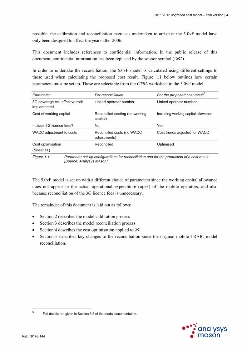
In order to undertake the reconciliation, the 5.0vF model is calculated using different settings to

those used when calculating the proposed cost result. Figure 1.1 below outlines how certain

parameters must be set up. These are selectable from the CTRL worksheet in the 5.0vF model.

Parameter For reconciliation For the proposed cost result5

3G coverage cell effective radii

implemented

Linked operator number Linked operator number

Cost of working capital Reconciled costing (no working

capital)

Including working capital allowance

Include 3G licence fees? No Yes

WACC adjustment to costs Reconciled costs (no WACC

adjustments)

Cost trends adjusted for WACC

Cost optimisation

(Sheet )

Reconciled Optimised

Figure 1.1: Parameter set-up configurations for reconciliation and for the production of a cost result [Source: Analysys Mason]

The 5.0vF model is set up with a different choice of parameters since the working capital allowance

does not appear in the actual operational expenditure (opex) of the mobile operators, and also

because reconciliation of the 3G licence fees is unnecessary.

The remainder of this document is laid out as follows:

Section 2 describes the model calibration process

Section 3 describes the model reconciliation process

Section 4 describes the cost optimisation applied to

Section 5 describes key changes to the reconciliation since the original mobile LRAIC model

reconciliation.

5 Full details are given in Section 3.5 of the model documentation.


Ref: 19176-144 .

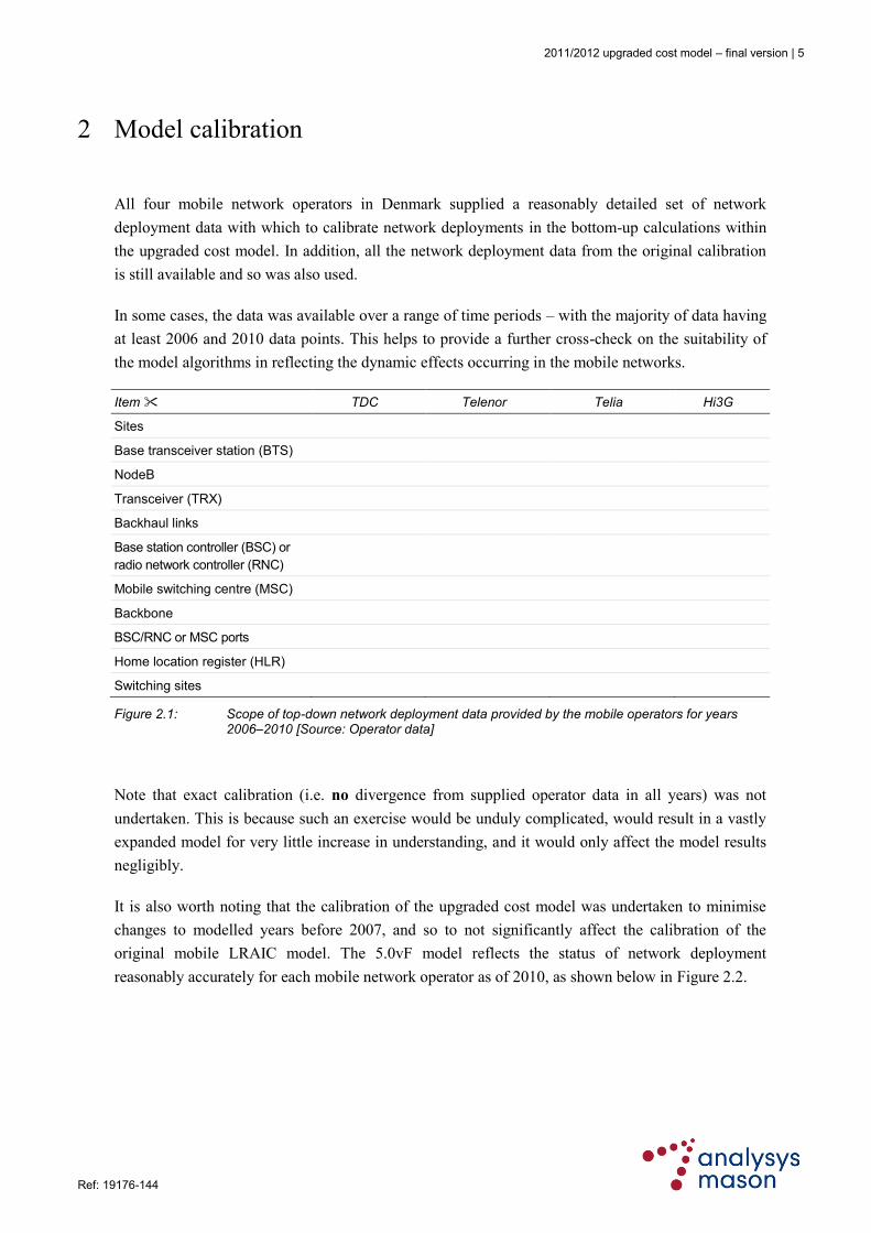
2 Model calibration

All four mobile network operators in Denmark supplied a reasonably detailed set of network

deployment data with which to calibrate network deployments in the bottom-up calculations within

the upgraded cost model. In addition, all the network deployment data from the original calibration

is still available and so was also used.

In some cases, the data was available over a range of time periods – with the majority of data having

at least 2006 and 2010 data points. This helps to provide a further cross-check on the suitability of

the model algorithms in reflecting the dynamic effects occurring in the mobile networks.

Item TDC Telenor Telia Hi3G

Sites

Base transceiver station (BTS)

NodeB

Transceiver (TRX)

Backhaul links

Base station controller (BSC) or

radio network controller (RNC)

Mobile switching centre (MSC)

Backbone

BSC/RNC or MSC ports

Home location register (HLR)

Switching sites

Figure 2.1: Scope of top-down network deployment data provided by the mobile operators for years 2006–2010 [Source: Operator data]

Note that exact calibration (i.e. no divergence from supplied operator data in all years) was not

undertaken. This is because such an exercise would be unduly complicated, would result in a vastly

expanded model for very little increase in understanding, and it would only affect the model results

negligibly.

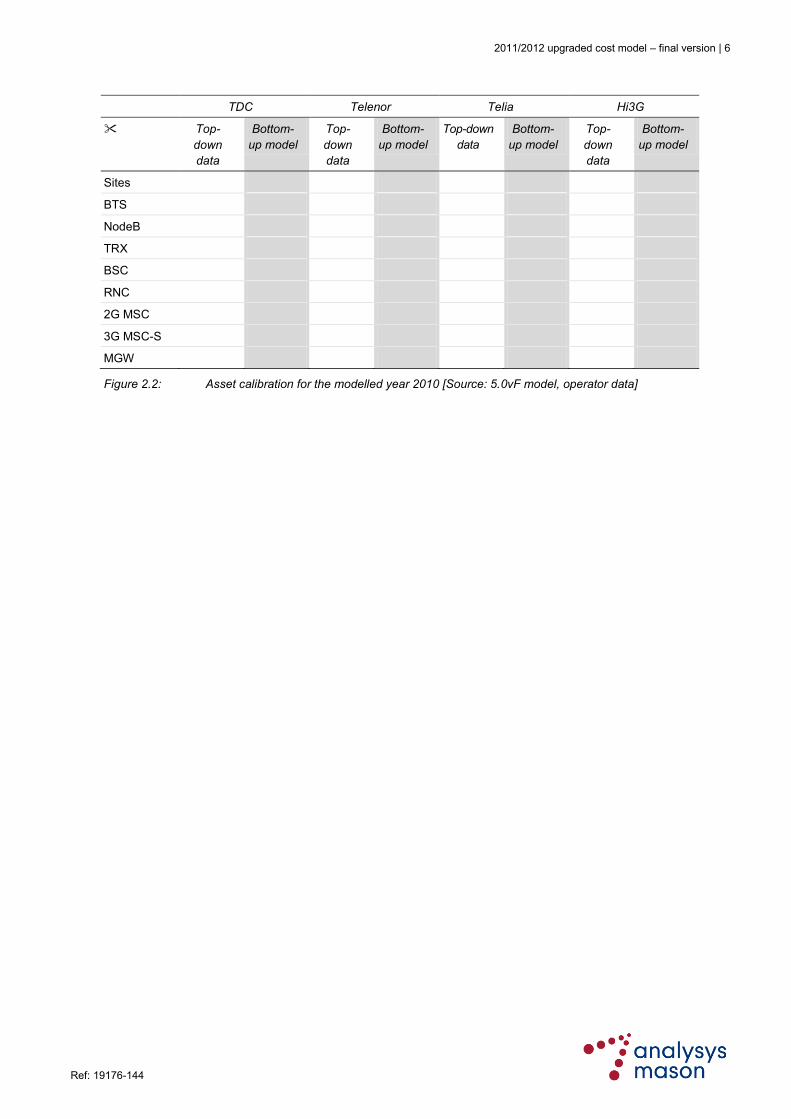
It is also worth noting that the calibration of the upgraded cost model was undertaken to minimise

changes to modelled years before 2007, and so to not significantly affect the calibration of the

original mobile LRAIC model. The 5.0vF model reflects the status of network deployment

reasonably accurately for each mobile network operator as of 2010, as shown below in Figure 2.2.


Ref: 19176-144 .

TDC Telenor Telia Hi3G

Top-

down

data

Bottom-

up model

Top-

down

data

Bottom-

up model

Top-down

data

Bottom-

up model

Top-

down

data

Bottom-

up model

Sites

BTS

NodeB

TRX

BSC

RNC

2G MSC

3G MSC-S

MGW

Figure 2.2: Asset calibration for the modelled year 2010 [Source: 5.0vF model, operator data]


Ref: 19176-144 .

3 Model reconciliation

Reconciliation of the bottom-up calculations within the upgraded cost model, as distinct from

calibration, is the process of comparing bottom-up expenditures of the model with top-down (actual)

expenditures submitted by the mobile operators. This reconciliation process can take into account

the breadth of expenditure information in the upgraded cost model:

unit capital prices of equipment

price trends

asset lifetimes

top-down capital expenditures (capex)

top-down opex

WACC.

The range of information provided in response to the data request issued to the Danish mobile

operators in June 2011 is presented below in Figure 3.1.6

Item TDC Telenor Telia Hi3G

Unit capital prices

Price trends

Asset lifetimes

Capex Yes Yes Yes Yes

Opex Yes Yes Yes Yes

Figure 3.1: Provision of reconciliation data [Source: Analysys Mason]

Accordingly, Analysys Mason‟s approach to reconciling the cost model utilised different methods in

each of these areas, as described below:

Unit capital prices

of equipment

The existing unit capital prices were in most cases kept unchanged from

the original mobile LRAIC model. The costs of equipment supplied by

were used as the basis of a check on the assumed capital prices for the

period 2007–2010. The two exceptions were the costs of owned site

acquisition and third-party site acquisition. In the original mobile LRAIC

model, for some (but not all) operators the costs of these two types of site

were set to be equal. In the 5.0vF model, the cost of owned site

acquisition has now been set higher than that for third-party site

acquisition in all cases.

Where new assets have been added to the 5.0vR model, the equipment

prices submitted by and international benchmarks (e.g. the unit costs

6 During the development of the original mobile LRAIC model, operators provided top-down data up to the end of 2006.

As part of the development of the 5.0vD model, data was requested for the period 2007–2011. This data was then used in conjunction with the data prior to 2006, in order to extend the reconciliation from 2006 to 2010.


Ref: 19176-144 .

in PTS‟s (the Swedish regulator) mobile LRIC model)7 have been used as

the basis of the direct equipment price for all operators. No new assets

have been added in the 5.0vF model.

Where operators, or benchmarks, have not provided necessary equipment

prices, Analysys Mason has developed its own estimates. In most cases,

these estimates were cross-checked (in aggregate) with the resulting top-

down cost data to ensure validity for the Danish context.

In addition to direct equipment prices, mobile operators undertake a wide

range of indirect capital investments – incremental upgrades, tools,

facilities, ancillary equipment, civil works, etc. These indirect costs do

not have a standard list price per unit, and therefore are usually only

identifiable from detailed asset register manipulation, business

plan/budgets or through top-down comparison. We have left the indirect

mark-ups used for the assets unchanged from the v4 model. For the new

assets (Ethernet backhaul, high-speed packet access (HSPA) upgrades

etc.), we have primarily used the cost model recently developed by PTS

in Sweden as a benchmark. None of these assets has a mark-up for

indirect costs in the PTS model and no data was provided by operators to

allow estimation of indirect mark-ups for these assets. Therefore, in the

5.0vF model, the indirect mark-ups are assumed to be zero.

We note that no operators provided unit prices for the operating costs of

assets.

Asset price trends The information on asset price trends supplied by operators concerned

capital equipment prices. To validate the existing annual price trends in

the model, the information provided by the mobile operators along with

Analysys Mason‟s estimates from other public mobile long-run

incremental cost (LRIC) models were compared.

Following this, a top-down comparison of capex and opex was

undertaken, applying cost trends between 2006–2010 to ensure that the

2006 unit prices had reach appropriate levels by 2010, based on the

information provided by .

Asset lifetimes The model uses economic lifetimes to drive the replacement of network

assets. The economic lifetimes in the original mobile LRAIC model were

based upon a number of information points:

typical mortgage durations in Denmark

economic lifetimes applied by the mobile cost model

7 http://www.pts.se/sv/Bransch/Telefoni/SMP---Prisreglering/Kalkylarbete-mobilnat/Gallande-prisreglering/.


Ref: 19176-144 .

Analysys Mason‟s estimates of the economic lifetime of network

elements in the absence of replacement, driven by accounting rules,

technology upgrade or service enhancement.

Although the model contains „accounting lifetimes‟ for reference, both

the reconciliation and the proposed cost result use „economic lifetimes‟.

In this way, assets are only replaced after their estimated useful life,

rather than after their average accounting lifetime.

For the 5.0vF model, no existing assets had their lifetimes revised. For the

new assets added to the model, economic lifetimes consistent with similar

existing assets were used.

Top-down capex We have been able to compare capex calculated by the model directly (in

nominal terms) with the data provided by all four operators. This was

performed at an aggregate and sub-category level in order to compare the

capital investments associated with each operator‟s business.

Top-down opex Due to the lack of bottom-up information on opex per network element

from the mobile operators, we have checked the total opex levels in the

model for each operator according to reconciliation with the categorised

top-down data.

Each of these areas is discussed in greater detail below.

3.1 Unit capital costs of equipment

The capital equipment cost for each network element was initially set in the reconciliation of the

original mobile LRAIC model, with values derived according to:

direct equipment prices from the price list information submitted by the mobile operators

the identification of additional indirect capital investments from the top-down accounting

information.

However, the upgraded cost model contains a number of entirely new assets in the asset list. To derive

unit costs for the entirely new assets, a similar process was undertaken as in generating the original asset

costs. Both the direct equipment prices from and international benchmarks (e.g. prices in PTS‟s

mobile LRIC model)8 were used as the basis for equipment prices.

Figure 3.2 below shows those assets in the upgraded cost model that have either been modified or are

entirely new. A color-coding system is used to illustrate the sources of information used to calculate

them.

Figure 3.2: Direct equipment prices [Source: 5.0vF model]

8 http://www.pts.se/sv/Bransch/Telefoni/SMP---Prisreglering/Kalkylarbete-mobilnat/Gallande-prisreglering/.


Ref: 19176-144 .

The colour-coding system used in Figure 3.2 is explained below.

Colour Description Figure 3.3: Colour scheme used in cost base inputs [Source: Analysys Mason]

Calculated from the bottom-up costs supplied by the

operator9

Based on bottom-up costs supplied by another operator

Derived from international benchmarks

Derived from actual top-down expenditures

Unit cost not required for that case

3.2 Asset price trends

In reconciling the asset price trends in the upgraded cost model, it was decided to consider the trends

after 2006 in two separate parts, namely the trends from 2006–2010 and the trends in the long term.

We describe these considerations separately below.

3.2.1 Price trends between 2006–2010

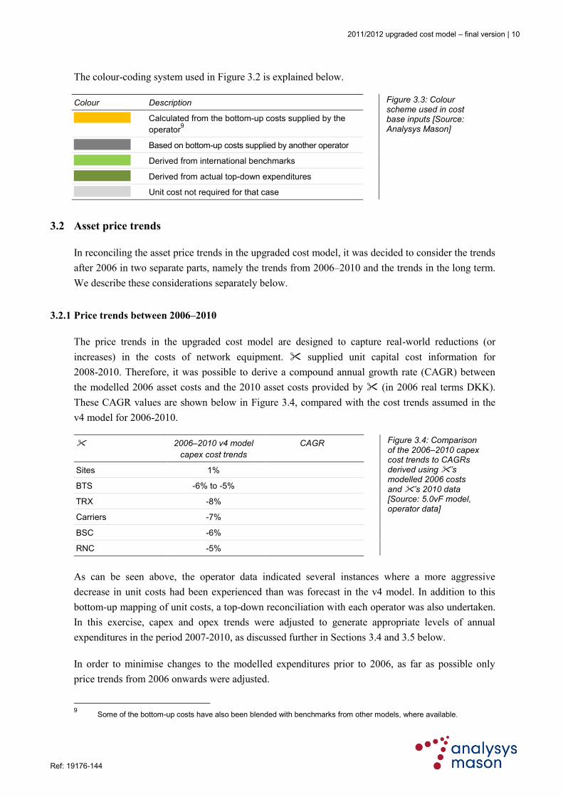
The price trends in the upgraded cost model are designed to capture real-world reductions (or

increases) in the costs of network equipment. supplied unit capital cost information for

2008-2010. Therefore, it was possible to derive a compound annual growth rate (CAGR) between

the modelled 2006 asset costs and the 2010 asset costs provided by (in 2006 real terms DKK).

These CAGR values are shown below in Figure 3.4, compared with the cost trends assumed in the

v4 model for 2006-2010.

2006–2010 v4 model

capex cost trends

CAGR Figure 3.4: Comparison of the 2006–2010 capex cost trends to CAGRs derived using ’s modelled 2006 costs and ’s 2010 data [Source: 5.0vF model, operator data]

Sites 1%

BTS -6% to -5%

TRX -8%

Carriers -7%

BSC -6%

RNC -5%

As can be seen above, the operator data indicated several instances where a more aggressive

decrease in unit costs had been experienced than was forecast in the v4 model. In addition to this

bottom-up mapping of unit costs, a top-down reconciliation with each operator was also undertaken.

In this exercise, capex and opex trends were adjusted to generate appropriate levels of annual

expenditures in the period 2007-2010, as discussed further in Sections 3.4 and 3.5 below.

In order to minimise changes to the modelled expenditures prior to 2006, as far as possible only

price trends from 2006 onwards were adjusted.

9 Some of the bottom-up costs have also been blended with benchmarks from other models, where available.


Ref: 19176-144 .

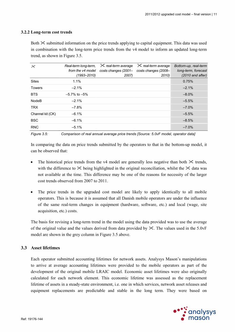
3.2.2 Long-term cost trends

Both submitted information on the price trends applying to capital equipment. This data was used

in combination with the long-term price trends from the v4 model to inform an updated long-term

trend, as shown in Figure 3.5.

Real-term long-term,

from the v4 model

(1993–2010)

real-term average

costs changes (2001–

2007)

real-term average

costs changes (2008–

2010)

Bottom-up, real-term

long-term, forecast

(2010 and after)

Sites 1.1% 0.75%

Towers –2.1% –2.1%

BTS –5.7% to –5% –8.0%

NodeB –2.1% –5.5%

TRX –7.8% –7.0%

Channel kit (CK) –6.1% –5.5%

BSC –6.1% –8.5%

RNC –5.1% –7.0%

Figure 3.5: Comparison of real annual average price trends [Source: 5.0vF model, operator data]

In comparing the data on price trends submitted by the operators to that in the bottom-up model, it

can be observed that:

The historical price trends from the v4 model are generally less negative than both trends,

with the difference to being highlighted in the original reconciliation, whilst the data was

not available at the time. This difference may be one of the reasons for necessity of the larger

cost trends observed from 2007 to 2011.

The price trends in the upgraded cost model are likely to apply identically to all mobile

operators. This is because it is assumed that all Danish mobile operators are under the influence

of the same real-term changes in equipment (hardware, software, etc.) and local (wage, site

acquisition, etc.) costs.

The basis for revising a long-term trend in the model using the data provided was to use the average

of the original value and the values derived from data provided by . The values used in the 5.0vF

model are shown in the grey column in Figure 3.5 above.

3.3 Asset lifetimes

Each operator submitted accounting lifetimes for network assets. Analysys Mason‟s manipulations

to arrive at average accounting lifetimes were provided to the mobile operators as part of the

development of the original mobile LRAIC model. Economic asset lifetimes were also originally

calculated for each network element. This economic lifetime was assessed as the replacement

lifetime of assets in a steady-state environment, i.e. one in which services, network asset releases and

equipment replacements are predictable and stable in the long term. They were based on


Ref: 19176-144 .

characteristics of the Danish market (e.g. typical mortgage durations) and the economic lifetimes

used by Ofcom (UK) and PTS (Sweden).

Additionally, in the original mobile LRAIC model, economic lifetimes were limited to a maximum

of 20 years to reflect a conservative view of long-lived assets. This principle has been maintained in

the 5.0vF model.

When determining the lifetimes for the new assets added to the 5.0vF model, values from existing

equivalent assets have been used, or benchmarks from other mobile cost models where this was not

possible.

3.4 Top-down capex

All four operators submitted categorised top-down capex. These actual data points were used to

assess the degree to which the direct bottom-up equipment prices managed to capture the levels of

expenditure actually accumulated by the mobile businesses.

The majority of new data received from operators was given in the format as outlined in the operator

data request. These categories where mapped to the existing broad capex categories, as shown in

Figure 3.6, so as to expand the previous reconciliations to 2010.

Data request TDC Telenor Telia Hi3G

Radio network

Last-mile backhaul

BSCs/RNCs

Transmission, excl.

backbone

Switching

Backbone

transmission

Other core

infrastructure

Indirect network

costs

Non-network costs

Business

overheads

Figure 3.6: Broad capex categories; note that the number of categories provided varies by operator [Source: Analysys Mason]

The aggregated direct bottom-up equipment prices, including both direct and indirect costs, have

been reconciled against the actual top-down expenditures given by operators. The cumulative capex

was compared as this removes possible timing effects from the expenditures. Figure 3.7 below


Ref: 19176-144 .

shows a comparison of the modelled cumulative capex versus the actual cumulative capex for each

operator.

TDC Telenor Telia10

Hi3G

Top-

down

Bottom-

up

Top-

down

Bottom-

up

Top-

down

Bottom-

up

Top-

down

Bottom-

up

Cumulative capex

to end 2006

% difference

Cumulative capex

to end 2010

% difference

Figure 3.7: Cumulative capex comparison for modelled direct and indirect expenditures (nominal DKK million) [Source: 5.0vF model, operator data]

3.5 Top-down opex

Given the limited availability of bottom-up unit opex applicable to the Danish mobile network

operators, the level of opex in the upgraded cost model has been set according to the available top-

down data. A comparison of total opex for the four mobile operators for both 2006 and 2010 is

shown below in Figure 3.8.

TDC Telenor Telia Hi3G

Top-

down

Bottom-

up

Top-

down

Bottom-

up

Top-

down

Bottom-

up

Top-

down

Bottom-

up

Total opex, 2006

% difference

Total opex, 2010

% difference

Figure 3.8: Comparison of total opex (nominal 2006 DKK million) [Source: 5.0vF model, operator data]

As is the case with capex, there have been no revisions made to the indirect opex mark-ups.

Similarly, there have been no indirect mark-ups derived for the new assets, due to lack of available

data. Instead, the direct cost is assumed to capture all associated operating costs for the asset.

10

In the development of the original mobile LRAIC model, did not provide a full-time series of in-year investments for

its historical investments. As an alternative, the present value of capex was calculated instead for the purposes of reconciliation instead.


Ref: 19176-144 .

4 Cost optimisation

In this section we revisit the cost optimisation previously applied to . We have compared the costs

calculated across TDC, Telenor and Telia in order to ascertain where network and costing differences

exist. Figure 4.1 shows the components of total cumulative economic costs (sum of capex and

opex over time) calculated with the unit costs applicable to each mobile operator. In this comparison

it is important to observe that the inventory of assets being considered in each case is identical; the

only difference is the unit capex and opex assumed.

Figure 4.1: Network costs under different unit cost situations [Source: 5.0vF model]

We note that this comparison still raises questions about the expenditure allocation provided by ,

since:

The last-mile access backhaul layer of the network exhibits a significant and material difference

when compared to costs calculated according to the cost bases of the other operators.

The proportion of capex, and hence termination costs, contributed by the appears high compared

to Analysys Mason‟s experience of this part of the cost base in similar cost models, and is

significantly higher than for the other Danish mobile operators.

fully reconciled expenditures are calculated using the following unit prices:

unit capex (1992) = direct capex (1992) plus indirect costs

unit opex (1992) = × unit capex (1992).

Based on our comparison between the mobile operators, we consider that costs in the 5.0vF

model should still be reduced by an indirect cost multiplier and a unit opex multiplier. This level of

unit costs for can therefore be considered fully optimal for the purpose of wholesale mobile

termination regulation in the Danish context.

When undertaking this analysis for the 5.0vD model, it was observed that Figure 4.1 showed a

significant change in the economic cost within “other core infrastructure” and “backbone

transmission” when using the cost base of Operator 1 (). The reason for the difference in

backbone transmission was that the unit opex for the “National site-site circuit switched backbone

distance (SDH STM1)” was almost an order of magnitude higher for than the other operators.

We reduced this level in the 5.0vD model, producing closer agreement for this category. This is also

accounted for in the opex reconciliation in Figure 3.8, and does not significantly affect the opex

reconciliation for . The reason for the difference in other core infrastructure (which can still be

seen in Figure 4.1 above) is primarily the higher costs assumed in the cost base for the voicemail


Ref: 19176-144 .

server and the billing system, compared with the other operators. We have not revised these inputs in

the calculation in the model, although this can be investigated further.


Ref: 19176-144 .

5 Updates to calibration and reconciliation of the cost model

This section describes some of the key changes to the model as a result of the calibration and

reconciliation of the actual operator calculations for TDC, Telenor, Telia and Hi3G for the years

2007–2010.

Section 5.1 describes updates made related to the calibration of modelled assets

Section 5.2 describes updates made related to the reconciliation of modelled expenditures

Section 5.3 describes modifications made as a result of deriving the 5.0vR model

Section 5.4 describes modifications made as a result of deriving the 5.0vF model.

5.1 Updates related to calibration in the 5.0vD model

Choice of 3G cell

radii used for

calibration

In the original reconciliation, the effective cell radii implemented for 3G

coverage was assumed to be „Draft v2 voice, outdoor‟. When either

calculating a cost result, or undertaking calibration/reconciliation, this input

is now set to „Linked operator number‟.

The reason for using „Draft v2 voice, outdoor‟ radii in the v4 model was that

urban indoor cell radii, as used in the cost result at the time, caused a rapid

deployment of sites, with the look-ahead effect in the model leading to 3G

costs being incurred in 2006 and 2007. In addition, 3G coverage was too

limited in order to adequately calibrate the 3G coverage inputs by operator

in the model.

In 2011, following four more years of evolution in the 3G networks in

Denmark, these 3G coverage inputs can now be more accurately calibrated.

This means that it can now be considered reasonable to use these radii

during calibration/reconciliation, thus aligning the 3G methodology with

that used for 2G.

Updated traffic

measures

The various proportions of daily traffic in the busy hour were updated with

more recent data for each operator. Although this affects the model results

prior to 2007, none of the parameters had changed significantly, meaning

that any differences to the calibration prior to 2006 were not substantial.

In addition, operator information was used to populate the 5.0vD model

busy-hour parameters for both Release 99 and HSPA.

Updated site splits The split of sites by owned tower, third-party tower and third-party rooftop

sites was updated for 2010 and 2011 using operator data. The number of

2G/3G indoor sites and repeaters in tunnels were also updated for each


Ref: 19176-144 .

operator.

Updated BSC/RNC

capacities

To update the BSC and RNC capacities in a similar fashion as described by

operators in their data submissions, a BSC and RNC „upgrade path‟ was

defined. This functionality is intended to represent the fact that both BSCs

and RNCs are available in a range of step-wise capacities, with operators

tending to deploy a mixture of capacities. Therefore, the capacity used in the

model each year becomes a weighted average of the capacity options.

Updated other

asset capacities

In addition to updating the BSC and RNC capacities, other assets‟ capacities

were revised only where necessary. Examples of such revision are the HLR

capacity for and the capacity of the SMS centre (SMSC) throughput for

.

Updated some

utilisation factors

During the calibration, some of the operators‟ utilisation factors were

updated. This was mostly related to 3G assets. Where utilisation factors

varied over time, such as that for the BSC, they were updated for the years

2007-2010.

Other updates In addition to the above, various smaller updates were made:

To capture a roll-out of HSPA across the network, the minimum speed

deployment for high-speed downlink packet access (HSDPA) for each

geotype was calibrated with operator data. Minimum speeds were

usually set so that the urban geotypes had equal speeds to, or faster than,

the suburban geotypes, which in turn had equal speeds to, or faster than,

the rural geotypes. The HSUPA grade deployed was then that

corresponding to the ladder of HSDPA speed deployed.

The percentage of pre-existing 2G sites available for 3G upgrade was

adjusted to match the data submitted by the mobile operators.

Call attempts per successful call and average call durations were checked

against the new operator information and adjusted where appropriate.

5.2 Updates related to reconciliation in the 5.0vD model

Choice of 3G cell

radii used for

reconciliation

This change, as described above, is also used to reconcile expenditures.


Ref: 19176-144 .

Used modelled

lifetimes rather

than accounting or

economic lifetimes

for reconciliation

We have used the modelled lifetimes for reconciliation rather than using

purely economic-based or purely accounting-based asset depreciation

lifetimes. We believe this is reasonable since we are modelling replacement

capex in the upgraded cost model, which should reflect the lifetimes of

assets enduring in the network, rather than when they are fully depreciated.

Revised unit capex

for existing assets

In response to data submission that the type of sites being purchased

change in value over time, site assets were further split down by geotype to

allow for their unit costs to vary by geotype. For the 5.0vD model, the unit

cost of a site is assumed to be the same in all four geotypes, which is

consistent with the v4 model.

The unit capex for owned sites and third-party sites has also been updated so

that the former has a higher unit cost than the latter for all operators (in the

original v4 model, these were set as equal for some operators).

Following the investigations in Section 4, unit opex for the “National

site-site circuit switched backbone distance (SDH STM1)” asset was

reduced to a level closer to that of the other operators.

Added unit costs for

new assets

New assets were added to the upgraded cost model including HSPA,

Ethernet backhaul, and an Ethernet backbone. The unit costs for these new

assets were calculated using a blend of benchmarking from other cost

models and cost data submitted by .

Revised 2006–2010

capex trends

The cost trends between 2006 and 2010 were revised, as described in

Section 3.2.1. To capture operator unit cost changes over this time,

significant negative cost trends had to be applied to many assets.

While the cost trends are more negative than usual, it is felt that in this

instance they are appropriate as they are only applied for a small number of

years. They are also indicated as appropriate in order to get closer top-down

reconciliation with actual opex. The long-term trend is more conservative

than these short-term reductions. In addition, both the mobile cost models

developed by Ofcom (in the UK) and ARCEP (in France) have precedents

for large negative trends in this time period.

Revised long-term

capex trends

The long-term capex trends were revised as is detailed in Section 3.2.2,

using operator data from , as well as international benchmarks.


Ref: 19176-144 .

Revised 2006–2010

opex trends

The opex cost trends between 2006 and 2010 were revised during the top-

down opex reconciliation to capture annual operator opex over this period.

To achieve similar opex charges as seen in operator data, significant

negative cost trends had to be applied to some of the asset classes, though as

with the capex trends this is felt to be reasonable over the short time period.

As is the case for capex, there are also precedents for negative price trends

(in real terms) from the models developed by both Ofcom and ARCEP.

Revised long-term

opex trends

The majority of long-term opex trends remained as in the original

calibration. New cost trends were added for new assets according to

benchmarks, or to be consistent with existing assets in the same asset class.

Adjustments to

operator data

Data supplied by operators was adjusted prior to calibration to ensure the

accuracy of the comparison. The key adjustments are listed below:

„indirect network‟ capex in 2010 was assumed to be the same as

in 2009, as otherwise there was a significantly inflated capex in

2010

„network transmission‟ opex in 2010 was assumed to be the

same as in 2006 to take into account having internalised

transmission costs

„interconnect‟, „handsets‟ and „depreciation and amortisation‟ opex

values were excluded from reconciliation data

the 2009 and 2010 „business overheads‟ capex for was assumed

to be the same as in 2008, to remove effects of

„non-network costs‟ were excluded from ‟s opex to better

correspond to its previous submission; „capitalised indirect network

costs‟ were included in the capex reconciliation.

5.3 Updates to the 5.0vR model

Adjusted

radii/SNOCC

values

The 3G SNOCC values in the model were adjusted for each operator to be

slightly more accurate. In addition, where 3G 2100MHz and 1800MHz

SNOCC values had been previously adjusted for calibration, these were

returned to the original calculated values.


Ref: 19176-144 .

Recalibrated 2G

base station assets

The model was adjusted so that operators which use 900MHz as their

primary spectrum (including the generic operator), had their secondary

1800MHz spectrum coverage profiles de-activated. This means that any

sites using 1800MHz spectrum are now fully traffic-driven.

As a result of these changes to the SNOCC, the 2G network asset calibration

for all three 2G operators had to be recalibrated. This was achieved by

modifying the BTS utilisation, the TRX utilisation and the “Proportion of

capacity driven additional sites by spectrum type.”

Revised long-term

opex trend for site

assets

The opex trend from 2010 onwards for site assets was revised from 0% to

0.45%, based on data from Danmarks Statistik.

Updated unit costs

for two operators

For , several asset unit capex costs were updated using recently supplied

data. In addition, the cost trends for Indoor_BTS, Tunnel_BTS and

NodeB_indoor were modified to retain reconciliation.

5.4 Updates to the 5.0vF model

Revised long-term

opex trend for site

assets

The cost trend for all site rental type charges were adjusted to follow a 3%

nominal cost trend (converted into real terms using the model‟s inflation

forecast).

Documents

2011/2012 upgraded cost model final version - · PDF file · 2014-12-02Report for the Danish Business Authority (DBA) 2011/2012 upgraded cost model – final version Reconciliation