Embed Size (px)
Citation preview

Calhoun: The NPS Institutional Archive
Theses and Dissertations Thesis Collection
2011-03
Authorship attribution of short messages
using multimodal features
Boutwell, Sarah R.
Monterey, California. Naval Postgraduate School
http://hdl.handle.net/10945/5813

NAVAL
POSTGRADUATE SCHOOL
MONTEREY, CALIFORNIA
THESIS
Approved for public release; distribution is unlimited
AUTHORSHIP ATTRIBUTION OF SHORT MESSAGES USING MULTIMODAL FEATURES
by
Sarah R. Boutwell
March 2011
Thesis Co-Advisors: Robert Beverly Craig H. Martell

THIS PAGE INTENTIONALLY LEFT BLANK

i
REPORT DOCUMENTATION PAGE Form Approved OMB No. 0704-0188Public reporting burden for this collection of information is estimated to average 1 hour per response, including the time for reviewing instruction, searching existing data sources, gathering and maintaining the data needed, and completing and reviewing the collection of information. Send comments regarding this burden estimate or any other aspect of this collection of information, including suggestions for reducing this burden, to Washington headquarters Services, Directorate for Information Operations and Reports, 1215 Jefferson Davis Highway, Suite 1204, Arlington, VA 22202-4302, and to the Office of Management and Budget, Paperwork Reduction Project (0704-0188) Washington DC 20503. 1. AGENCY USE ONLY (Leave blank)
2. REPORT DATE March 2011
3. REPORT TYPE AND DATES COVERED Master’s Thesis
4. TITLE AND SUBTITLE Authorship Attribution of Short Messages Using Multimodal Features 6. AUTHOR(S) Sarah R. Boutwell
5. FUNDING NUMBERS
7. PERFORMING ORGANIZATION NAME(S) AND ADDRESS(ES) Naval Postgraduate School Monterey, CA 93943-5000
8. PERFORMING ORGANIZATION REPORT NUMBER
9. SPONSORING /MONITORING AGENCY NAME(S) AND ADDRESS(ES)
N/A
10. SPONSORING/MONITORING AGENCY REPORT NUMBER
11. SUPPLEMENTARY NOTES The views expressed in this thesis are those of the author and do not reflect the official policy or position of the Department of Defense or the U.S. Government. IRB Protocol number: n/a ________________. 12a. DISTRIBUTION / AVAILABILITY STATEMENT Approved for public release; distribution is unlimited
12b. DISTRIBUTION CODE
13. ABSTRACT (maximum 200 words) In this thesis, we develop a multimodal classifier for authorship attribution of short messages. Standard natural language processing authorship attribution techniques are applied to a Twitter text corpus. Using character n-gram features and a Naïve Bayes classifier, we build statistical models of the set of authors. The social network of the selected Twitter users is analyzed using the screen names referenced in their messages. The timestamps of the messages are used to generate a pattern-of-life model. We analyze the physical layer of a network by measuring modulation characteristics of GSM cell phones. A statistical model of each cell phone is created using a Naïve Bayes classifier. Each phone is assigned to a Twitter user, and the probability outputs of the individual classifiers are combined to show that the combination of natural-language and network-feature classifiers identifies a user to phone binding better than when the individual classifiers are used independently.
15. NUMBER OF PAGES
187
14. SUBJECT TERMS Authorship Attribution, Machine Learning, Twitter, GSM, Device Identification, Multimodal Classifier, Naïve Bayes
16. PRICE CODE
17. SECURITY CLASSIFICATION OF REPORT
Unclassified
18. SECURITY CLASSIFICATION OF THIS PAGE
Unclassified
19. SECURITY CLASSIFICATION OF ABSTRACT
Unclassified
20. LIMITATION OF ABSTRACT
UU NSN 7540-01-280-5500 Standard Form 298 (Rev. 2-89) Prescribed by ANSI Std. 239-18

ii
THIS PAGE INTENTIONALLY LEFT BLANK

iii
Approved for public release; distribution is unlimited
AUTHORSHIP ATTRIBUTION OF SHORT MESSAGES USING MULTIMODAL FEATURES
Sarah R. Boutwell Lieutenant, United States Navy
B.S., Johns Hopkins University, 1996
Submitted in partial fulfillment of the requirements for the degree of
MASTER OF SCIENCE IN COMPUTER SCIENCE
from the
NAVAL POSTGRADUATE SCHOOL March 2011
Author: Sarah R. Boutwell
Approved by: Robert Beverly Thesis Co-Advisor
Craig H. Martell Thesis Co-Advisor
Peter J. Denning Chair, Department of Computer Science

iv
THIS PAGE INTENTIONALLY LEFT BLANK

v
ABSTRACT
In this thesis, we develop a multimodal classifier for
authorship attribution of short messages. Standard natural
language processing authorship attribution techniques are
applied to a Twitter text corpus. Using character n-gram
features and a Naïve Bayes classifier, we build statistical
models of the set of authors. The social network of the
selected Twitter users is analyzed using the screen names
referenced in their messages. The timestamps of the
messages are used to generate a pattern-of-life model. We
analyze the physical layer of a network by measuring
modulation characteristics of GSM cell phones. A
statistical model of each cell phone is created using a
Naïve Bayes classifier. Each phone is assigned to a
Twitter user, and the probability outputs of the individual
classifiers are combined to show that the combination of
natural-language and network-feature classifiers identifies
a user to phone binding better than when the individual
classifiers are used independently.

vi
THIS PAGE INTENTIONALLY LEFT BLANK

vii
TABLE OF CONTENTS
I. INTRODUCTION ............................................1 A. IDENTITY ISSUES ....................................1 B. RESEARCH QUESTIONS .................................3 C. SIGNIFICANT FINDINGS ...............................3 D. ORGANIZATION OF THESIS .............................4
II. BACKGROUND ..............................................7 A. INTRODUCTION .......................................7 B. TWITTER ............................................7
1. Twitter Attributes ............................8 C. PRIOR WORK IN AUTHORSHIP ATTRIBUTION ...............9
1. Lexical Feature Analysis ......................9 2. N-Gram Feature Analysis ......................11
D. PRIOR WORK IN DEVICE IDENTIFICATION ...............15 1. Signal Transient Characteristic Method .......16 2. Steady State Signal Characteristic Method ....17 3. Modulation Characteristic Method .............19 4. Transport Layer Characteristic Method ........21
E. GSM OVERVIEW ......................................22 1. GSM Network Infrastructure ...................23 2. Mobile Handset ...............................24 3. GSM Modulation ...............................25
F. MACHINE LEARNING TECHNIQUES .......................27 1. Naïve Bayes Classifier .......................28 2. Smoothing ....................................30
a. Laplace Smoothing .......................30 b. Witten-Bell Smoothing ...................31
3. Combining Classifiers ........................31 G. EVALUATION CRITERIA ...............................35
III. TECHNIQUES .............................................39 A. INTRODUCTION ......................................39 B. CORPUS GENERATION .................................39
1. Twitter Streaming ............................39 2. Text Data Collection and Processing ..........40
C. AUTHORSHIP ATTRIBUTION PROCESS ....................42 1. Feature Extraction ...........................43 2. Naïve Bayes Classifier .......................45
D. PATTERN OF LIFE ANALYSIS ..........................46 1. Twitter Time Analysis ........................46 2. Social Network Analysis ......................47
E. CELL PHONE SIGNAL ANALYSIS ........................48 1. Signal Collection ............................48 2. Data Analysis and Classification .............52

viii
F. COMBINING CLASSIFIERS .............................53 IV. RESULTS AND ANALYSIS ...................................57
A. TEXT RESULTS ......................................57 B. PATTERN OF LIFE RESULTS ...........................67 C. SOCIAL NETWORK RESULTS ............................69 D. PHONE SIGNAL ANALYSIS .............................71 E. COMBINED CLASSIFIERS ..............................73 F. DETECTING AUTHOR CHANGES ..........................80
V. CONCLUSIONS ............................................89 A. SUMMARY ...........................................89 B. FUTURE WORK .......................................92
1. Social Network Analysis ......................92 2. Other Machine Learning Methods ...............92 3. Expanded Phone Signal Analysis ...............93 4. Segmentation Inside Boundaries ...............93 5. Temporal Posting Aspects .....................94
C. CONCLUDING REMARKS ................................94 APPENDIX A: MEASURING GSM PHASE AND FREQUENCY ERRORS .....97 APPENDIX B: ADDITIONAL TEXT CLASSIFICATION DATA .........101 APPENDIX C: TWEET SEND TIME ADDITIONAL DATA .............113 APPENDIX D: PHONE CLASSIFIER ADDITIONAL DATA ............123 APPENDIX E: COMBINED CLASSIFIER ADDITIONAL DATA .........141 LIST OF REFERENCES .........................................159 INITIAL DISTRIBUTION LIST ..................................163

ix
LIST OF FIGURES
Figure 1. Typical Twitter Message..........................9 Figure 2. Comparison of Several Authorship Attribution
Techniques on Different Textual Domains (After [10], [11], [12], [3])..........................15
Figure 3. QPSK Error Shown on an I/Q Plane (From [4]).....20 Figure 4. Vector Display of Modulation Errors (From [4])..20 Figure 5. GSM Network Structure (From [19])...............23 Figure 6. GMSK Modulation Block Diagram (From [23]).......26 Figure 7. GMSK Demodulation Block Diagram (From [23]).....27 Figure 8. Naïve Bayes Classification Process..............43 Figure 9. NPSML Format....................................44 Figure 10. Date/Time Field Format..........................46 Figure 11. Cell Control Screen (From [35]).................49 Figure 12. Data Bits Screen (From [35])....................50 Figure 13. Phase and Frequency Error Screen (Multi-burst
on)(From [35])..................................51 Figure 14. Classification Accuracy for 50 Authors Using
150 Tweets per Author With Increasing Document Size............................................61
Figure 15. Classification Accuracy for 50 Authors by Document Size and Total Number of Tweets per Author..........................................61
Figure 16. Classification Accuracy Results for Various Total Tweet Values Per Author With Increasing Author Count....................................62
Figure 17. Classification Accuracy Results for Various Author Counts With Increasing Total Tweet Per Author Values...................................63
Figure 18. Classification Results for 20 Authors With Varying Values of Tweets per Author and Tweets per Document....................................64
Figure 19. Classification Results for 20 Authors With More Than 100 Tweets per Author and Varying Tweets per Document....................................65
Figure 20. Classification Accuracy for 50 Authors of 120 Tweet Times per Author With Increasing Number of Tweet Times per Training Set.................68
Figure 21. Classification Accuracy Results for Social Network Analysis of 120 @names per Author With Increasing Number of @names per Training Set....70
Figure 22. Classification Accuracy for 20 Devices With Varying Vectors per Training Set and Total Vectors per Device..............................72

x
Figure 23. Classification Accuracy Results for 20 Phones With 150 Data Vectors and Varying Document Size.73
Figure 24. Classification Accuracy of Individual and Combined Classifiers for 30 Tweets/Signal Vectors and Various Training Set Sizes..........74
Figure 25. Classification Accuracy of Individual and Combined Classifiers for 50 Tweets/Signal Vectors and Various Training Set Sizes..........75
Figure 26. Classification Accuracy of Individual and Combined Classifiers for 100 Tweets/Signal Vectors and Various Training Set Sizes..........75
Figure 27. Classification Accuracy of Individual and Combined Classifiers for 120 Tweets/Signal Vectors and Various Training Set Sizes..........76
Figure 28. Classification Accuracy of Individual and Combined Classifiers for 150 Tweets/Signal Vectors and Various Training Set Sizes..........76
Figure 29. GMSK Phase Error Measurement (From [38])........98 Figure 30. GMSK Modulation Errors and Specified Limits
(From [38]).....................................99 Figure 31. Author 1045 Tweet Send Time Histogram..........113 Figure 32. Author 1388 Tweet Send Time Histogram..........113 Figure 33. Author 1734 Tweet Send Time Histogram..........114 Figure 34. Author 1921 Tweet Send Time Histogram..........114 Figure 35. Author 2546 Tweet Send Time Histogram..........115 Figure 36. Author 2744 Tweet Send Time Histogram..........115 Figure 37. Author 3155 Tweet Send Time Histogram..........116 Figure 38. Author 3693 Tweet Send Time Histogram..........116 Figure 39. Author 5599 Tweet Send Time Histogram..........117 Figure 40. Author 5742 Tweet Send Time Histogram..........117 Figure 41. Author 6111 Tweet Send Time Histogram..........118 Figure 42. Author 6886 Tweet Send Time Histogram..........118 Figure 43. Author 7100 Tweet Send Time Histogram..........119 Figure 44. Author 7241 Tweet Send Time Histogram..........119 Figure 45. Author 7754 Tweet Send Time Histogram..........120 Figure 46. Author 7958 Tweet Send Time Histogram..........120 Figure 47. Author 8164 Tweet Send Time Histogram..........121 Figure 48. Author 8487 Tweet Send Time Histogram..........121 Figure 49. Author 9417 Tweet Send Time Histogram..........122 Figure 50. Author 9800 Tweet Send Time Histogram..........122 Figure 51. Averaged Accuracy Results of Normalized
Combined Classifiers for Each Phone-Author Pairing Matrix Using One Tweet per Training Set157
Figure 52. Averaged Accuracy Results of Normalized Combined Classifiers for Each Phone-Author

xi
Pairing Matrix Using Three Tweets per Training Set............................................157
Figure 53. Averaged Accuracy Results of Non-Normalized Combined Classifiers for Each Phone-Author Pairing Matrix Using One Tweet per Training Set158
Figure 54. Averaged Accuracy Results of Non-Normalized Combined Classifiers for Each Phone-Author Pairing Matrix Using Three Tweets per Training Set............................................158

xii
THIS PAGE INTENTIONALLY LEFT BLANK

xiii
LIST OF TABLES
Table 1. Collection Quantities...........................41 Table 2. Top Five n-grams................................44 Table 3. Classification Accuracy Results for 50 Authors
With 230 Tweets Per Author......................58 Table 4. Classification Accuracy Results for 50 Authors
With 120 Tweets Per Author With Comparison to SCAP Method.....................................58
Table 5. Classification Accuracy Results for 50 Authors With 230 Tweets per Author Combined into Documents of Size 23 Tweets.....................59
Table 6. Classification Accuracy Results for 50 Authors Using 10 Documents With Increasing Number of Tweets per Document.............................60
Table 7. Classification Accuracy Results for Single Tweet Documents Tested on Models Trained on Multi-Tweet Documents of the Specified Quantity.66
Table 8. Classifier Accuracy Results for Each Author Using 120 Tweet Times per Author and Increasing Number of Tweet Times per Training Set..........69
Table 9. Comparing Combination of Probability Logarithms and Combination of Normalized Probability Logarithms......................................77
Table 10. Normalized Probability Logarithm Combination Resulting in Incorrect Classification...........79
Table 11. Confusion Matrix for Text Classifier for Simulated Author Change Using 50 Tweets per Author With One Tweet per Document With Ten Tweets Exchanged Between Authors................82
Table 12. Confusion Matrix for Text Classifier for Simulated Author Change Using 50 Tweets per Author With Three Tweets per Document With Nine Tweets Exchanged Between Authors................82
Table 13. Confusion Matrix for Text Classifier for Simulated Author Change Using 120 Tweets per Author With Five Tweets per Document With 25 Tweets Exchanged Between Authors................83
Table 14. Classification Accuracy of Text Classifier for Simulated Author Change – True Positives (non-swap) and False Positives (Swap)................83
Table 15. Confusion Matrix for Normalized Combined Classifier for Simulated Author Change Using 50 Tweets per Author With One Tweet per Document With Ten Tweets Exchanged Between Authors.......84

xiv
Table 16. Confusion Matrix for Normalized Combined Classifier for Simulated Author Change Using 50 Tweets per Author With Three Tweets per Document With Nine Tweets Exchanged Between Authors.........................................84
Table 17. Confusion Matrix for Normalized Combined Classifier for Simulated Author Change Using 120 Tweets per Author With Five Tweets per Document With 25 Tweets Exchanged Between Authors.........................................85
Table 18. Confusion Matrix for Non-normalized Combined Classifier for Simulated Author Change Using 50 Tweets per Author With One Tweet per Document With Ten Tweets Exchanged Between Authors.......85
Table 19. Confusion Matrix for Non-normalized Combined Classifier for Simulated Author Change Using 50 Tweets per Author With Three Tweets per Document With Nine Tweets Exchanged Between Authors.........................................86
Table 20. Confusion Matrix for Non-normalized Combined Classifier for Simulated Author Change Using 120 Tweets per Author With Five Tweets per Document With 25 Tweets Exchanged Between Authors.........................................86
Table 21. Classification Accuracy of Combined Classifiers for Detecting Simulated Author Change – True Positives (non-swap) and False Positives (Swap).87
Table 22. Confusion Matrix for 30 Tweets per Author With One Tweet per Document.........................101
Table 23. Confusion Matrix for 30 Tweets per Author With Three Tweets per Document......................102
Table 24. Confusion Matrix for 50 Tweets per Author With One Tweet per Document.........................103
Table 25. Confusion Matrix for 50 Tweets per Author With Three Tweets per Document......................104
Table 26. Confusion Matrix for 50 Tweets per Author With Five Tweets per Document.......................105
Table 27. Confusion Matrix for 120 Tweets per Author With One Tweet per Document.........................106
Table 28. Confusion Matrix for 120 Tweets per Author With Three Tweets per Document......................107
Table 29. Confusion Matrix for 120 Tweets per Author With Five Tweets per Document.......................108
Table 30. Confusion Matrix for 150 Tweets per Author With One Tweet per Document.........................109

xv
Table 31. Confusion Matrix for 150 Tweets per Author With Three Tweets per Document......................110
Table 32. Confusion Matrix for 150 Tweets per Author With Five Tweets per Document.......................111
Table 33. Per Author Accuracy Rates for Various Total Tweets per Author and Tweets per Document......112
Table 34. Confusion Matrix for 30 Signal Vectors per Phone With One Signal Vector per Training Set..123
Table 35. Confusion Matrix for 30 Signal Vectors per Phone With Two Signal Vectors per Training Set.124
Table 36. Confusion Matrix for 30 Signal Vectors per Phone With Three Signal Vectors per Training Set............................................125
Table 37. Confusion Matrix for 50 Signal Vectors per Phone With One Signal Vector per Training Set..126
Table 38. Confusion Matrix for 50 Signal Vectors per Phone With Two Signal Vectors per Training Set.127
Table 39. Confusion Matrix for 50 Signal Vectors per Phone With Three Signal Vectors per Training Set............................................128
Table 40. Confusion Matrix for 50 Signal Vectors per Phone With Four Signal Vectors per Training Set129
Table 41. Confusion Matrix for 50 Signal Vectors per Phone With Five Signal Vectors per Training Set130
Table 42. Confusion Matrix for 100 Signal Vectors per Phone With One Signal Vector per Training Set..131
Table 43. Confusion Matrix for 100 Signal Vectors per Phone With Two Signal Vectors per Training Set.132
Table 44. Confusion Matrix for 100 Signal Vectors per Phone With Three Signal Vectors per Training Set............................................133
Table 45. Confusion Matrix for 120 Signal Vectors per Phone With One Signal Vector per Training Set..134
Table 46. Confusion Matrix for 120 Signal Vectors per Phone With Two Signal Vectors per Training Set.135
Table 47. Confusion Matrix for 120 Signal Vectors per Phone With Three Signal Vectors per Training Set............................................136
Table 48. Confusion Matrix for 150 Signal Vectors per Phone With One Signal Vector per Training Set..137
Table 49. Confusion Matrix for 150 Signal Vectors per Phone With Two Signal Vectors per Training Set.138
Table 50. Confusion Matrix for 150 Signal Vectors per Phone With Three Signal Vectors per Training Set............................................139

xvi
Table 51. Per Phone Accuracy Rates for Various Total Signal Vectors per Phone and Vectors per Training Set...................................140
Table 52. Phone to Author Pairing Matrix.................141 Table 53. Confusion Matrix for Normalized Combined
Classifier Matrix Pairing 1 Using 30 Tweets/Signal Vectors With One Tweet/Signal Vector per Training Set........................142
Table 54. Confusion Matrix for Non-normalized Combined Classifier Matrix Pairing 1 Using 30 Tweets/Signal Vectors With One Tweet/Signal Vector per Training Set........................143
Table 55. Confusion Matrix for Normalized Combined Classifier Matrix Pairing 1 Using 30 Tweets/Signal Vectors With Three Tweets/Signal Vectors per Training Set.......................144
Table 56. Confusion Matrix for Non-normalized Combined Classifier Matrix Pairing 1 Using 30 Tweets/Signal Vectors With Three Tweets/Signal Vectors per Training Set.......................145
Table 57. Confusion Matrix for Normalized Combined Classifier Matrix Pairing 1 Using 50 Tweets/Signal Vectors With One Tweet/Signal Vector per Training Set........................146
Table 58. Confusion Matrix for Non-normalized Combined Classifier Matrix Pairing 1 Using 50 Tweets/Signal Vectors With One Tweet/Signal Vector per Training Set........................147
Table 59. Confusion Matrix for Normalized Combined Classifier Matrix Pairing 1 Using 50 Tweets/Signal Vectors With Three Tweets/Signal Vectors per Training Set.......................148
Table 60. Confusion Matrix for Non-normalized Combined Classifier Matrix Pairing 1 Using 50 Tweets/Signal Vectors With Three Tweets/Signal Vectors per Training Set.......................149
Table 61. Confusion Matrix for Normalized Combined Classifier Matrix Pairing 1 Using 120 Tweets/Signal Vectors With One Tweet/Signal Vector per Training Set........................150
Table 62. Confusion Matrix for Non-normalized Combined Classifier Matrix Pairing 1 Using 120 Tweets/Signal Vectors With One Tweet/Signal Vector per Training Set........................151
Table 63. Confusion Matrix for Normalized Combined Classifier Matrix Pairing 1 Using 120

xvii
Tweets/Signal Vectors With Three Tweets/Signal Vectors per Training Set.......................152
Table 64. Confusion Matrix for Non-normalized Combined Classifier Matrix Pairing 1 Using 120 Tweets/Signal Vectors With Three Tweets/Signal Vectors per Training Set.......................153
Table 65. Confusion Matrix for Normalized Combined Classifier Matrix Pairing 1 Using 120 Tweets/Signal Vectors With Five Tweets/Signal Vectors per Training Set.......................154
Table 66. Confusion Matrix for Non-normalized Combined Classifier Matrix Pairing 1 Using 120 Tweets/Signal Vectors With Five Tweets/Signal Vectors per Training Set.......................155
Table 67. Per Pair Combined Classifier Accuracy Results by Total Tweets/Signal Vectors and Tweets/Signal Vectors per Training Set.........156

xviii
THIS PAGE INTENTIONALLY LEFT BLANK

xix
LIST OF ACRONYMS AND ABBREVIATIONS
3GPP 3rd Generation Partnership Project
API Application Programming Interface
ARFCN Absolute Radio Frequency Channel Number
BSC Base Station Controller
BTS Base Transceiver Station
ETSI European Telecommunications Standards Institute
FDM Frequency Division Multiplexing
FPGA Field-Programmable Gate Array
GMSK Gaussian Minimum-Shift Keying
GMT Greenwich Mean Time
GSM Global System for Mobile Communications
I/Q In-phase/Quadrature
ICMP Internet Control Message Protocol
IMEI International Mobile Equipment Identifier
IMSI International Mobile Subscriber Identity
JSON JavaScript Object Notation
kNN k-Nearest Neighbor
MAC Media Access Control
NIC Network Interface Card
NPSML Naval Postgraduate School Machine Learning
NRZ Non-Return-To-Zero
PARADIS Passive Radiometric Device Identification System
PCH Physical Channel
PSTN Public Switched Telephone Network
QPSK Quadrature Phase Shift Keying
RF Radio Frequency
RMS Root Mean Square
SCAP Source Code Author Profiles
SIM Subscriber Identity Module
SMS Short Message Service

xx
SVM Support Vector Machine
TacBSR Tactical Base Station Router
TCP Transport Control Protocol
TDM Time Division Multiplexing
UMOP Unintentional Modulation on Pulse
URL Uniform Resource Locator
WARP Wireless Open-Access Research Platform
XML Extensible Markup Language

xxi
ACKNOWLEDGMENTS
I would like to acknowledge the many people who helped
make this work possible. I would like to thank my advisors
Professor Rob Beverly and Professor Craig Martell. Without
your guidance and insight, this work would not have been
possible, and Professor Beverly’s critical eye and rigor
helped make this an excellent product.
I would like to thank the other members of my cohort
for the support in finishing this program. Particularly, I
would like to thank the other members of the Natural
Language Processing Lab, CDR Jody Grady, LT Charles Ahn, LT
Randy Honaker, and LT Kori Levy-Minzie for help with
software and all the shared suffering.
I would also like to thank Brandon for all the moral
support through this process.

xxii
THIS PAGE INTENTIONALLY LEFT BLANK

1
I. INTRODUCTION
The cellular telephone has become ubiquitous.
Teenagers carry them to school, and adults carry them to
work. They provide connection and communication,
information and entertainment. In the U.S., 93% of the
population has access to a cell phone, and 24.5% of
households have abandoned the landline to use cellular only
[1]. Along with the cell phone, the short messaging
service (SMS) has also gained popularity. Americans sent
7.2 billion SMS messages a month in 2005. In 2010, that
value increased to 173.2 billion a month. The annualized
value of 1.81 trillion text messages a year comes close to
matching the 2.26 trillion minutes of cell phone use in
2010 [1]. SMS messages are an integral part of modern
communication.
A. IDENTITY ISSUES
The benefits and convenience of SMS messaging,
however, bring with them new difficulties for human
identity. For example, one can answer a phone call and
immediately detect that it is one’s sister on the other end
of the line by the sound of her voice. However, upon
receiving a text message from one’s sister, it may be her,
or she may have her husband key the message while she is
driving. While this is an innocuous example of an identity
mismatch, it is easy to imagine more malicious behavior.
Identity is a crucial part of network security.
Devices communicate their identity to a network at the
network link layer in the form of a media access control
(MAC) address; cell phones on a Global System for Mobile

2
Communications (GSM) network use an international mobile
equipment identifier (IMEI). A sophisticated adversary can
falsify or “spoof” these identification codes to appear as
a different device. Users authenticate to the network at
the application layer in the form of passwords or biometric
information. Passwords have well-known vulnerabilities if
they are not carefully selected, and biometrics have not
achieved widespread use. Users can access web-based
applications from any internet-capable device, allowing
independence from a specific platform.
For authentication mechanisms in cell phone networks,
the provider mandates the user have a physical token in the
form of a registered phone or subscriber identity module
(SIM) card to gain access to the network. Even this notion
of “registration” is not uniformly employed. Legislators
in the Philippines just introduced a bill in January 2011
regulating the sale and distribution of SIM cards.
Currently, pre-paid SIM cards and cellular phones can be
purchased in the Philippines and many other countries,
without having to provide any identification or register a
legal name with a network provider. More trivially, phones
may also be lost or misappropriated. Thus, it is difficult
to tie a cell phone used in an illegal activity, such as a
kidnapping, with its user [2].
A registration system may improve accountability in
cell phone use, but policy alone cannot guarantee that the
name in the database associated with a phone is the same
person using the phone at any point in time. This identity
uncertainty can also be problematic in situations that do
not involve illegal activities. A business that issues

3
cell phones to its employees may not want those phones used
for non-work-related communications. A government agency
may want an unobtrusive way to ensure that an employee has
not lost or loaned his phone to a family member. In these
situations, an authority wants to establish and monitor a
device-to-user binding, associating a specific user to a
specific phone. Beyond security, a phone that is
contextually aware may wish to display specific information
or act differently depending on the user. We propose that
it is possible to identify the user of a mobile wireless
device based on the statistical analysis of user’s text
messaging characteristics and their phones’ radio
transmission signals.
B. RESEARCH QUESTIONS
This thesis addresses two questions related to
identity determination on mobile devices. We first examine
whether combining user-specific text authorship
characteristics and device-specific signal characteristics
in a naïve Bayes classifier improves upon the accuracy
results of classifying these characteristics individually.
The second question asks if this classifier can detect when
a phone normally used by one individual begins to be used
by a different individual. We use an authorship
attribution analysis of the text of short messages as the
user classifier, and an analysis of signal modulation
characteristics as the device classifier.
C. SIGNIFICANT FINDINGS
This research produced the following significant
results:

4
• Classification of 120 individual Twitter messages from 50 authors using a multiclass naïve Bayes classifier produced 40.3% authorship attribution accuracy, less than the 54.4% found by Layton, Watters, and Dazeley using the Source Code Author Profiles (SCAP) method [3].
• Combining multiple Twitter messages to generate a text feature vector for input to the classifier improves authorship attribution accuracy. Using a feature vector from 23 combined messages produces the best result of 99.6% accuracy.
• Classification of 120 individual cell phone radio signal modulation characteristic vectors for 20 GSM cell phones resulted in a 90% classification accuracy. This compares favorably to the 99% accuracy of Brik et al. for modulation characteristics of 802.11 devices [4].
• Sum rule combination of the text and phone classifiers improves upon the results of the text classifier. Multimodal classifier accuracies over 99% were attained when using individual classifiers that employed the method of combining multiple messages to create the input feature vectors.
• The multimodal classifier was able to detect a simulated new user on a phone 36% of the time in the best-performing configuration.
D. ORGANIZATION OF THESIS
This thesis is organized as follows:
• Chapter I discusses the difficulty of ascertaining identity on mobile devices and the research questions we address in our experimentation.
• Chapter II discusses prior work in authorship attribution, device identification, and the machine learning techniques used in this study.
• Chapter III describes the methods used to collect and process data and set up and execute the classification experiments.

5
• Chapter IV contains the results of the experiments and analysis of their significance.
• Chapter V contains conclusions drawn from the results and possible areas of future research.

6
THIS PAGE INTENTIONALLY LEFT BLANK

7
II. BACKGROUND
A. INTRODUCTION
Developing a binding between a user and a device
involves merging the efforts to classify the user by
applying authorship attribution methods, e.g., statistical
word counts, social network structure, etc., and to
classify the device using the characteristics of its
wireless signal. This chapter describes the textual and
signal domains that provide our data. We discuss
authorship attribution and device identification
techniques, followed by an overview of machine learning
classification methods. A description of the software
tools used in this research concludes the chapter.
B. TWITTER
Twitter provides a popular “microblogging” service,
allowing users to communicate with messages of 140
characters or less known as tweets. Users subscribe to
another user’s message “feed” to “follow” them, receiving
messages from the user they follow. Twitter also provides
a mechanism for users to reply to a tweet, directly send a
message to another user, or repeat a received tweet to
their own set of followers, thereby expanding the
readership of that tweet. Users have the option to specify
that their tweets are private, viewable only by their
followers or the direct recipient of a tweet, or publicly
viewable. Users post their messages to Twitter via
twitter.com, text messages, or third party clients,
including mobile applications. As of September 14, 2010,
Twitter reports it has 175 million users, while 95 million

8
tweets are sent per day [5]. We expect Twitter, and
Twitter-like services, to continue to gain in popularity
and that our work will be relevant to not only Twitter, but
to new services that emerge.
1. Twitter Attributes
Twitter’s primary characteristic that differentiates
it from e-mail, chat, or a standard blog is its 140-
character length limit. In this respect, tweets have more
in common with short message service (SMS) messages than
any other communication technology [6]. Many language
conventions of chat and SMS such as abbreviated spellings,
acronyms, misspellings, and emoticons (i.e., combinations
of characters that represent emotions, for instance a
smiley face using a colon and a right parenthesis) are also
used extensively in Twitter. While some misspellings are
accidental, others are for effect, such as writing
“sleeeepy” instead of “sleepy.” Another technique we note
in our examination of our Twitter corpus is the chat
convention where writers use asterisks before and after a
statement to indicate action, for example “really? *bangs
head on desk*.” The similarities noted between SMS and
Twitter text imply that analysis methods that work in one
domain will also work in the other.
Twitter adds two unique message attributes beyond SMS:
the @ sign followed by a user’s screen name to indicate a
reference to that user, and the # sign followed by a topic
tag for use in grouping and searching messages by topic
thread. We shall refer to these attributes as @names and
#tags. In [7], Boyd, et al. found that, in a random sample
of 720,000 tweets, 36% of them contain a @name and 5%

9
contain a #tag. Figure 1 is an anonymized example of a
tweet using these attributes. In this example, the sender
directs the tweet to @User1 in a conversational manner,
referencing @User2 within the comment.
Figure 1. Typical Twitter Message
Another common message attribute is the Internet URL.
As a text-only communication medium, Twitter users include
Uniform Resource Locator (URL) links to outside content
they wish to share [8]. This practice has given rise to
URL shorteners, services such as http://bit.ly that provide
redirection from a longer standard URL to a shortened URL
(i.e., http://bit.ly/a1b2c3), enabling more efficient use
of the limited message space.
C. PRIOR WORK IN AUTHORSHIP ATTRIBUTION
Authorship attribution takes a piece of written
material and attempts to identify its author. Typically,
this is done through a supervised learning process, taking
material known to be written by an author and building a
model from it, then gauging how well the writing in
question fits the model. Researchers have found different
ways to build these models. A discussion of several of
these techniques follows, with an emphasis on those that
have shown success with short messages.
1. Lexical Feature Analysis
Lexical features treat the text as a series of tokens,
with a token consisting of a word, number, or punctuation
@User1 no wonder @User2 never wrote me back #epicfail

10
mark, or some combination of alphanumeric characters. The
author model consists of statistics such the distribution
of sentence length, vocabulary richness, word frequencies,
etc. An example of vocabulary richness is the ratio of the
number of unique words in a corpus to the total number of
words in the corpus. Vectors built from word frequencies
that include the most common words, such as prepositions
and pronouns, represent the author’s style, and are most
often used in authorship detection. When vectors discard
high frequency words with little semantic content, those
prepositions and pronouns tend to perform better in topic
detection [9].
In her 2007 thesis, Jane Lin used lexical features to
profile authors of the NPS Chat Corpus by age and gender.
In the processing of her corpus, she grouped Internet chat
utterances by the age reported in the user’s profile,
maintaining punctuation marks intact. This allowed her to
build a dictionary of common emoticons and use them as a
feature for classification. In her analysis she used the
following features: emoticon token counts, emoticon types
per sentence, punctuation token counts, punctuation types
per sentence, average sentence length, and average count of
word types per document (vocabulary richness). She used a
naïve Bayes classifier, which we describe later, to compute
classification accuracy both with and without prior
probability [10].
Lin found that while classifying teens against 20-
year-olds showed poor results, comparing them to
increasingly older age groups improved the results. The
top F-score, a metric of combined precision and recall that

11
we detail later, of 0.932 came from comparing teens to 50-
year-olds. As most sexual predators are 26 and older, she
compared those under 26 to those over 26 with a resulting
F-score of 0.702. Based on the results and her data, she
suggested that other machine learning techniques may
perform better [10].
2. N-Gram Feature Analysis
While the use of word features captures the style of
the author well, it fails to capture certain features
common to short messaging. Emoticons, abbreviations, and
creative punctuation use may carry morphological
information useful in stylistic discrimination. Custom-
built parsers, such as used by Lin in the work described
above, could pull these features out of the text but add a
level of complexity to tokenizing and smoothing [9]. An
alternative approach uses character-level n-grams as the
feature type. This method disregards language-specific
information such as word spacing, letter case, or new line
markers. It also eliminates the need for taggers, parsers,
or any other complex text preprocessing.
In [11], Keselj et al. used byte-level n-grams for
authorship attribution of English, Greek, and Chinese
texts. For each author they built a profile of the L most
common character n-grams and their normalized frequencies.
The basic theory of this method is that authorship is
determined by the amount of similarity between the profiles
of two texts, classifying a test profile as the author
profile from which it is least dissimilar. The measure of
dissimilarity is a normalized distance metric based on the
n-gram frequencies within the text profiles. They refer to

12
this measurement as the relative distance between two
texts. For English texts by eight classic authors, they
achieved 100% accuracy for several different n-gram and
profile sizes. On Greek data sets drawn from newspaper
texts they attained an accuracy of 85%, surpassing the
previous best reported accuracy of 73% for that data set.
These results suggest that byte-level n-grams have some
useful application in authorship attribution.
Keselj’s method of determining the difference between
two author profiles of byte-level n-gram features was
expanded upon and simplified by [12] in order to apply the
technique to a different textual domain. Instead of the
normalized distance metric used by Keselj to differentiate
authors, Frantzeskou et al. built profiles of the L most
common n-grams used by the authors of computer source code
samples. Unlike the previous method, this approach does
not normalize the n-gram frequencies. They call this the
Source Code Author Profiles (SCAP) method. The size of the
set of n-grams in the intersection of the two author
profile sets measures the distance between the authors. A
test document gets classified as the author with whom this
intersection set is largest.
Frantzeskou et al. used a corpus of C++ programs
applying Keselj’s method and the SCAP method to data from
six authors. While results were similarly good for both
methods with 100% accuracy at higher profile size (L)
values, or number of n-grams per author, SCAP performed
slightly better at lower values of L, and significantly
better with bi-grams. On a corpus consisting of Java code
with no comments, SCAP again performed better with

13
accuracies from 92 – 100% across several values of L and n-
gram sizes. The relative distance method performed well at
lower values of L, but poorly at the highest L value tested
[12]. The SCAP method provides a mathematically simple and
effective means of conducting authorship attribution on
source code material. While computer program source code
and short messages have very different structures, both
domains may present at first glance the impression of very
broken, oddly punctuated English. Although Twitter covers
a wider vocabulary range, authorship attribution methods
effective in one domain may show similar effectiveness in
the other.
The success of the SCAP method with source code led to
an examination by [3] of its viability for authorship
attribution of short messages, specifically those sent via
Twitter. Layton, Watters, and Dazeley examined 50 users
randomly from a set of 14,000. The 140-character limit of
Twitter messages restricted the amount of unique characters
sufficiently that they used a value of L that encompassed
all characters used by an author. The value of n was
varied from 2 to 7 characters. The experiment used three
different text preprocessing methods to gauge the effect of
the tagging conventions unique to Twitter, with one method
removing @names from the text, one removing #tags, and one
removing both.
Applying the SCAP methodology to Twitter produced a
best result of 72.9% accuracy using character 4-grams and
with both @names and #tags included in the message text.
The @name influenced results the most, showing an average
26% accuracy drop when removed. The #tags reduced accuracy

14
by only 1% on average. This implies that the inclusion of
user social network analysis can significantly improve the
ability to identify that user. The threshold number of
tweets per author beyond which accuracy did not
significantly improve was found to be 120. This study
showed that authorship attribution of short messages with
the SCAP method performs much better than chance, with the
addition of information on the user’s social network
significantly improving the classification performance [3].
As short messages sent via SMS do not generally contain
this social network information, their best accuracy result
of 54.4% with both @names and #tags removed is a more
realistic benchmark for authorship attribution of short
messages.
This subsection described several different methods
for authorship attribution in a variety of textual domains.
Figure 2 summarizes the key points discussed.

15
Figure 2. Comparison of Several Authorship Attribution
Techniques on Different Textual Domains (After [10], [11], [12], [3])
D. PRIOR WORK IN DEVICE IDENTIFICATION
Accurate identification of individuals on a network is
an important security concern. A number of security
exploits involve mimicking an authorized user to gain
access to a network. There is a parallel problem of trying
to identify individuals involved in nefarious activities
who may be trying to obfuscate their communications
activities by routinely changing devices or otherwise
misrepresenting themselves on a communications network. A
passive means of correctly identifying an authorized device
and its user by means of network characteristics,
electronic emissions, and/or textual analysis could

16
minimize the impact of spoofing attacks and contribute to
intelligence or law enforcement efforts to track a specific
individual.
Research in the 802.11 wireless domain shows that
individual devices can be identified quite well by their
radiometric signatures, even among users with the same
brand of device. This is due to inherent variability in
the manufacturing process. Other research has focused on
authorship attribution based on analysis of an individual’s
language use. No known research to date has combined the
two identification methods in an effort to improve the
classification of users to devices in a network. This study
will attempt to do so, with a focus on wireless and
cellular SMS communications.
Identification of radio frequency (RF) transmitters by
their signal characteristics has been accomplished with
good success, particularly in the radar domain. That
technology has advanced from basic measures of frequency,
amplitude, and pulse width to fine-grained analysis of
unintentional modulation on pulse (UMOP), which looks at
pulse artifacts unique to individual transmitters. Once a
radar is positively identified as transmitting a signal,
that radar can be identified by that signal in the future.
Unknown radars can be classified by manufacturer. A Litton
Applied Technology UMOP analysis method was able to
identify radars at 90—95% confidence level in the early
1990s [13].
1. Signal Transient Characteristic Method
Communications and data signals can be more complex
than radars, with different modulation schemes, spread
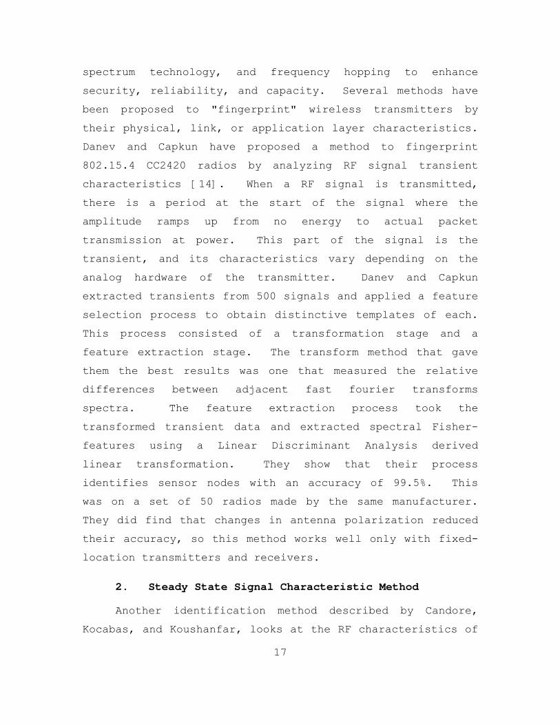
17
spectrum technology, and frequency hopping to enhance
security, reliability, and capacity. Several methods have
been proposed to "fingerprint" wireless transmitters by
their physical, link, or application layer characteristics.
Danev and Capkun have proposed a method to fingerprint
802.15.4 CC2420 radios by analyzing RF signal transient
characteristics [14]. When a RF signal is transmitted,
there is a period at the start of the signal where the
amplitude ramps up from no energy to actual packet
transmission at power. This part of the signal is the
transient, and its characteristics vary depending on the
analog hardware of the transmitter. Danev and Capkun
extracted transients from 500 signals and applied a feature
selection process to obtain distinctive templates of each.
This process consisted of a transformation stage and a
feature extraction stage. The transform method that gave
them the best results was one that measured the relative
differences between adjacent fast fourier transforms
spectra. The feature extraction process took the
transformed transient data and extracted spectral Fisher-
features using a Linear Discriminant Analysis derived
linear transformation. They show that their process
identifies sensor nodes with an accuracy of 99.5%. This
was on a set of 50 radios made by the same manufacturer.
They did find that changes in antenna polarization reduced
their accuracy, so this method works well only with fixed-
location transmitters and receivers.
2. Steady State Signal Characteristic Method
Another identification method described by Candore,
Kocabas, and Koushanfar, looks at the RF characteristics of

18
the steady-state part of the signal for unique elements
imparted by transmitter hardware [15]. They do this by
developing individual classifiers that may be weak for the
following characteristics: frequency difference, magnitude
difference, phase difference, distance vector, and I/Q
origin offset, where difference/distance/offset refers to
difference between the ideal values and actual measured
values of the signal. These individual classifiers are
then combined with weighted voting to form a stronger
classifier. Their work uses a Wireless Open-Access
Research Platform (WARP) built around a computer, field-
programmable gate array (FPGA) for the digital signal
processing, and radio cards operating in the 2.4 GHz and 5
GHz bands. They use Differential Quadrature phase-shift
keying modulation and extract their signal signatures in
the modulation domain. After training the classifier on
data collected from 200 frames of 1844 random symbols, they
then use five frames to test it. At five frames, results
were rather poor for six different radios. Testing with at
least 25 frames, the individual characteristic classifiers
each surpassed 50% identification accuracy. Combining the
classifiers with weighted voting, they got 88% accuracy
with a 12.8% false alarm probability of correct transmitter
identification on five frames. One reason they suggested
for the less than perfect identification results is that
their WARP radio cards contain many digital components,
which would have less inherent variability than other
radios with more analog components in the transmission
processing stream. If that is true, our software-oriented
test system may show the same signal stability.

19
3. Modulation Characteristic Method
The modulation domain was used again in a paper by
Brik et al., this time applied to 802.11 network interface
cards (NIC) [4]. They developed a methodology called the
passive radiometric device identification system (PARADIS).
Four of the five characteristics they used were the same as
in the WARP paper: frequency error, I/Q origin offset,
magnitude error, and phase error. They also used another
characteristic called SYNC correlation, which is the
difference between the measured and ideal I/Q values of the
SYNC, the short signal used to synchronize the transmitter
and receiver prior to transmitting the data. The 802.11
physical layer, in many instances, encodes data with two
sub-carriers, in-phase (I) and quadrature (Q) that are
separated by π/2. In quadrature phase shift keying (QPSK),
each symbol encodes two data bits and is represented by
points in the modulation domain using a constellation
diagram that plots the points in each of the four quadrants
of a two-dimensional grid. Errors in modulation are
usually measured by comparing vectors corresponding to the
I and Q values at a point of time. Phase error is the
angle between the ideal and measured phasor. Error vector
magnitude is magnitude of vector difference between ideal
and measured phasor. Those errors are taken as averages
across all symbols in the frame in order to minimize the
effects of channel noise. Figures 3 and 4 are a graphical
display of the error measurements.

20
Figure 3. QPSK Error Shown on an I/Q Plane (From [4])
Figure 4. Vector Display of Modulation Errors (From [4])
For their experiment, the Brik group used identical
Atheros NICs configured as 802.11b access points and an
Agilent vector signal analyzer as the sensor. They tried
both a k-Nearest Neighbor (kNN) and support vector machine
(SVM) classification schemes to associate a MAC address to
a NIC based on the collected modulation parameters. After
evaluating data from 138 NICs, the best feature set was
found to be, in order, frequency error, SYNC correlation,

21
I/Q offset, magnitude and phase errors for SVM. Freq
error, SYNC correlation, I/Q offset for kNN. The SVM
classifier error rate was 0.34%, and kNN classifier error
rate was 3%. Based on their data, no one NIC was able to
masquerade as another. Modulation similarities were under
5% for 99% of the cards. One NIC had a similarity to
others of 17% [4]. They also suggest that this method
could work with any digital modulation scheme.
4. Transport Layer Characteristic Method
A passive fingerprinting technique proposed by Kohno,
Broido, and Claffy, eschews the physical layer signal
analysis, instead exploiting the transport layer for
identity information by measuring clock skew in transport
control protocol (TCP) timestamps [16]. Their method
exploits two clocks on a computer: the system time clock
and a TCP timestamps option clock internal to the TCP
network stack. The system time clock may or may not be
synchronized with true time by connection to a Network Time
Protocol server. If not, the difference between system
time and true time can be measured. Most modern operating
systems enable the TCP timestamps option in their network
stack. Thus, each TCP packet sent contains a 32-bit
timestamp embedded in the packed header. They describe
methods for passively collecting TCP timestamps from
computers running various operating systems and formulas
for calculating clock skew from the timestamps. They also
describe a method for estimating system clock skew by
sending Internet control message protocol ICMP Timestamp
Requests to a targeted device, but focus on the TCP method,
as most network stacks use clocks operating at lower

22
frequencies than system clocks. Also, many routers and
firewalls filter ICMP messages. For clock skew measurement
to be effective, different devices must have different
clock skews, and the skews must be consistent over time.
Others have shown that both those assumptions hold, but
they prove it by collecting two hours of traffic on a major
link and using their process to find the clock skew of the
first hour, second hour, and entire period and comparing
them for each source that was active at least 30 minutes of
each hour. A plot of their findings found that they were
able to differentiate between some individual machines by
their clock skew, but not all. This is an interesting
method but not useful in our research, as cell phones
synchronize their clocks with their network upon
connection.
E. GSM OVERVIEW
The Global System for Mobile Communications (GSM)
standard is the basis for the most popular mobile phone
system in the world, with over 3 billion connections [17].
Its ubiquity and well-established hardware technology make
it a good platform for experimentation and a good target
for exploitation. GSM operates as a cellular network with
a set of base stations distributed over a service area.
The distribution is based on the desired coverage level,
which depends on geography and connection demand. A rural
area may have a few, high powered base stations spread out
over a large area, while an urban area might have many
lower powered units in close proximity [18]. The structure
of a GSM network is shown in Figure 1. The two left blocks
of Figure 1 contain the part of the network relevant to

23
this study: the handset, the base transceiver station
(BTS), and the air, or Um, interface between the two.
Figure 5. GSM Network Structure (From [19])
1. GSM Network Infrastructure
In a GSM network, the BTS contains the antennas, the
transceivers for transmitting and receiving RF signals, and
encryption gear as needed. While the complete capabilities
of the BTS vary depending on the network provider, the
minimum function is to receive the modulated analog RF
signal from the handset, convert it to a modulated digital
signal, and send it to the base station controller (BSC).
The BTS can contain more functionality, to include handling
handover between cells. The BTS is controlled by the BSC,
which typically controls several BTSs in a network. The
BSC manages the frequency channels used by its towers,
handles handovers and switching among its towers, and may
do the conversion from the air interface’s voice channel
coding to the coding used in the circuit-switched Public

24
Switched Telephone Network (PSTN) [20]. A small and simple
limited network can be assembled using only a BTS with
appropriate software to manage a specific number of
handsets. The network assembled for the experimentation
conducted here is one such limited network.
2. Mobile Handset
The end of the cellular wireless network most familiar
to typical users is the handset. Along with a transceiver
and digital signal processing unit, a GSM handset also
contains the subscriber identity module (SIM) card. The
SIM card is what identifies the user to the network,
allowing the network to choose to provide or deny access to
the user. A user can easily switch phones and still access
their subscribed services by transferring their SIM card to
the new phone, assuming that phone is unlocked and
compatible with the network technology. The indentifying
feature of the SIM card is the International Mobile
Subscriber Identity (IMSI) number. Each SIM card has a
unique IMSI associated to the user. The phone itself also
has a unique identifier, the International Mobile Equipment
Identity (IMEI) number [20]. These two numbers are
unrelated, though both may be transmitted through the
network as part of control signal metadata.
The air interface between the handset and the BTS is
the focus of part of the experimentation conducted here.
GSM providers operate in the licensed 450 MHz, 850 MHz, 900
MHz, 1800 MHz, and 1900 MHz radio frequency bands. Uplink
and downlink bands are typically each 25 MHz wide and
separated by 45 – 50 MHz. Each of these bands is divided
into 124 carrier frequencies with a 200 kHz bandwidth. An

25
uplink/downlink channel pair is referred to by an absolute
radio frequency channel number (ARFCN). Time-division
multiplexing is used to divide each channel into eight time
slots. A single timeslot in a specific ARFCN is called a
physical channel (PCH) [21]. Thus, GSM combines FDM and
TDM to make the most efficient use of its spectrum
assignment. Each timeslot, or burst, generally consists of
two 57 bit data fields separated by a 26 bit “training
sequence” for equalization, three tail bits at each end,
and an 8.25 bit guard sequence. Gaussian Minimum-Shift
Keying (GMSK) is the signal modulation scheme used to
modulate the digital data into the analog RF signal [21].
3. GSM Modulation
GSM uses the Gaussian Minimum Shift Keying modulation
scheme. This modulation method applies a Gaussian filter
to the data signal prior to the MSK modulator. MSK is a
form of digital frequency modulation with a 0.5 modulation
index. It has several properties that make it good for
efficient mobile radio use: a constant envelope, a narrow
bandwidth, and coherent detection capability. This makes
it relatively impervious to noise. The one thing it lacks
is the ability to minimize energy occurring out-of-band in
transmission. The Gaussian filter has a narrow bandwidth
and the cutoff properties to minimize extraneous
frequencies, shaping the input data waveform so that the
output fits a constant envelope. The single channel per
carrier characteristic of GSM, with carriers spaced 200 kHz
apart, minimizes off-carrier energy, and thus the Gaussian
filter is important to clear transmission [22].

26
The modulation sequence of a typical GMSK signal
modulator is shown in Figure 6. In this example, a stream
of binary data formed in a Non-Return-To-Zero (NRZ)
sequence is sampled and integrated into an analog signal.
It is then convoluted with a Gaussian function to filter
out the energy outside the Gaussian form. The real, in
phase (I) and quadrature (Q) components of the data signal
are calculated, then modulated onto the I and Q carrier
waves. The two components are added, and the modulated
signal is formed [23].
Figure 6. GMSK Modulation Block Diagram (From [23])
Demodulation of the GMSK signal is more complicated,
particularly for GSM applications. Operating in the 900
MHz range, GSM is subject to a significant amount of
interference, to include signal attenuation, multipath
propagation, and co-channel or adjacent band interference.
The GSM standard does not specify a demodulation algorithm,
but does say that it has to be able to handle two multipath
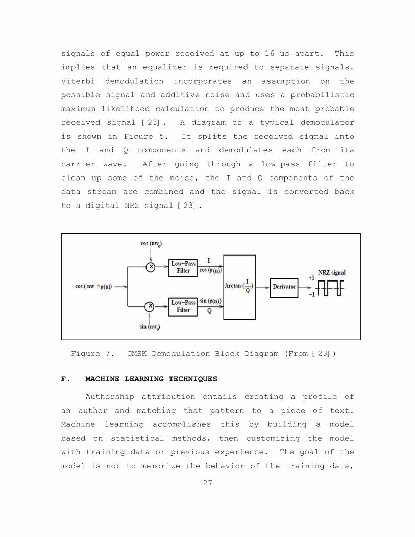
27
signals of equal power received at up to 16 µs apart. This
implies that an equalizer is required to separate signals.
Viterbi demodulation incorporates an assumption on the
possible signal and additive noise and uses a probabilistic
maximum likelihood calculation to produce the most probable
received signal [23]. A diagram of a typical demodulator
is shown in Figure 5. It splits the received signal into
the I and Q components and demodulates each from its
carrier wave. After going through a low-pass filter to
clean up some of the noise, the I and Q components of the
data stream are combined and the signal is converted back
to a digital NRZ signal [23].
Figure 7. GMSK Demodulation Block Diagram (From [23])
F. MACHINE LEARNING TECHNIQUES
Authorship attribution entails creating a profile of
an author and matching that pattern to a piece of text.
Machine learning accomplishes this by building a model
based on statistical methods, then customizing the model
with training data or previous experience. The goal of the
model is not to memorize the behavior of the training data,

28
but to use it to decide if new data points fit into the
pattern. While there are many machine learning techniques
based on different statistical mechanisms, this research
employs naïve Bayes.
1. Naïve Bayes Classifier
The naïve Bayes classifier uses Bayes’ Rule of
probability to assign a given set of features to a class.
( | ) ( )( | )( )
P C P CP CP
=FF
F
Bayes’ rule is particularly useful in many practical
situations where it is easier to estimate the conditional
probability of a particular feature given a class. The
conditional probability of the class given the features,
P(C|F), depends on the probabilities of the class and the
features and the probability of the features given the
class. When F is a vector of d random feature values, F =
(f1,…,fj,…,fd), and all documents fall into one of n random
classes conditional on the feature set, C = (c1,…,ck,…,cn),
Bayes’ Rule may be expressed as [24]:
( | ) ( )( | )( )k k
kP c P cP c
P=
FFF
The classification problem becomes simple when P(ck|F)
is known; as discussed in [10], [25], and [26] the document
with feature vector F is assigned to the class with the
highest conditional probability value, c*:
( | ) ( )* arg max( )k
k k
c C
P c P ccP∈
⎡ ⎤= ⎢ ⎥
⎣ ⎦
FF
29
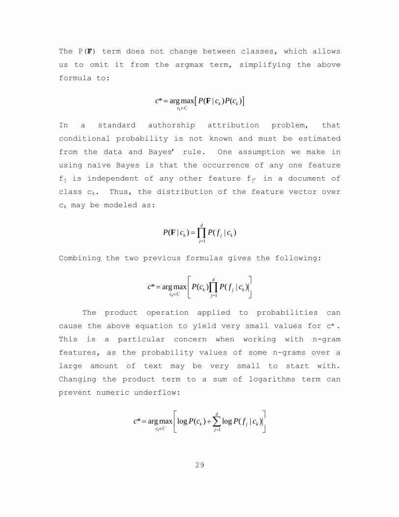
The P(F) term does not change between classes, which allows
us to omit it from the argmax term, simplifying the above
formula to:
[ ]* arg max ( | ) ( )k
k kc C
c P c P c∈
= F
In a standard authorship attribution problem, that
conditional probability is not known and must be estimated
from the data and Bayes’ rule. One assumption we make in
using naïve Bayes is that the occurrence of any one feature
fj is independent of any other feature fj’ in a document of
class ck. Thus, the distribution of the feature vector over
ck may be modeled as:
1
( | ) ( | )d
k j kj
P c P f c=
=∏F
Combining the two previous formulas gives the following:
1
* arg max ( ) ( | )k
d
k j kc C j
c P c P f c∈ =
⎡ ⎤= ⎢ ⎥
⎣ ⎦∏
The product operation applied to probabilities can
cause the above equation to yield very small values for c*.
This is a particular concern when working with n-gram
features, as the probability values of some n-grams over a
large amount of text may be very small to start with.
Changing the product term to a sum of logarithms term can
prevent numeric underflow:
1* arg max log ( ) log ( | )
k
d
k j kc C j
c P c P f c∈ =
⎡ ⎤= +⎢ ⎥
⎣ ⎦∑

30
The P(ck) term reflects the prior probability of the
class occurring in the data set. This is typically modeled
in one of two ways: as a uniform distribution of classes,
or as the actual proportion of the count of the class in
the training data. A training set containing equal
occurrences of four classes gives a prior probability of
0.25. One in which half the class occurrences belong to c1
gives that class a prior probability of 0.5. Thus the
balance of classes in the training data affects the naïve
Bayes classifier result.
2. Smoothing
The naïve Bayes classifier builds a probabilistic
model of a class based on training data from that class. A
problem arises when the test data contains features that
the model has not seen in training. These zero counts have
a zero probability, leaving the naïve Bayes classifier
unable to predict a class. Smoothing, the process of
shifting probability mass from frequently appearing
features to zero count features while retaining their
relative influence on the classifier, mitigates this
problem. Two smoothing techniques, Laplace and Witten-
Bell, are discussed here.
a. Laplace Smoothing
A simple algorithm, Laplace smoothing adds a
value of 1 to each feature count in the data set, both test
and training. This prevents a zero probability situation
by ensuring every feature has a probability of occurring
based on at least a single count, even if it does not
appear in the training data. Adding to the feature counts

31
requires a similar adjustment in the normalization step.
If N is the total count of all tokens in the data set and V
is the count of unique tokens, or types, a total of V is
added to the individual counts by adding 1 to each [26].
The normalization must also be adjusted by V for a Laplace
probability formula for a term:
1( ) iLaplace i
cP tN V+
=+
b. Witten-Bell Smoothing
Instead of altering the count of all features in
the data set, Witten-Bell uses the probabilities of the
features occurring in the training set to estimate the
probability of an unseen feature. As the training set is
processed, the probability that the next token will be of
type i is given by [27]:
( ) iW B i
cP tn v− =+
where n is the number of tokens seen so far and v is the
number of types seen so far. The total probability of an
unseen type occurring next is based on the fact that it has
already occurred v times in the training set and given by
[27]:
( )W B novelvP t
n v− =+
3. Combining Classifiers
A classifier for detecting a device to user binding
must derive information from both the user and the device.
In this research, the user is modeled by their short
message writing style and the device is modeled by signal

32
characteristics. The variety of features used makes it
mathematically difficult to simply plug them all into one
high-dimensional classifier, though it is possible with
appropriate normalization of the data. The fields of
biometrics, image analysis, and handwriting analysis also
use diverse feature sets for classification of target
items. Researchers in these fields have developed methods
to combine multiple classifiers, each focusing on a single
feature type, into a multimodal classifier system producing
accuracy rates superior to those of the individual
classifiers used independently.
Design of a multimodal classifier depends on the
outputs of the individual input classifiers. When
combining single class labels, a majority vote scheme may
be used. The class labels output by each component
classifier are counted, with the class that collects the
most votes selected as the output of the combined
classifier [28]. Variants of this system may apply
weights, potentially learned, to the inputs to the combined
classifier based on a quality metric or require the winning
class to have more than a simple majority. Input
classifiers providing a set of ranked class labels use a
combined classifier that joins the individual sets and re-
ranks the labels, selecting the top-ranked label as the
output [29].
The input classifiers that generate the greatest
amount of classification information provide the
probability distribution of the class labels, such as the
posterior probabilities produced by a Bayesian classifier.
[29] shows how the output probabilities Pk(Ci|x) of several

33
Bayesian classifiers may be averaged to create posterior
probabilities of the combined classifier:
1
1( | ) ( | )K
E i k ik
P C P CK =
= ∑x x
where i ranges from 1 to M classes and k from 1 to K
classifiers. The class selected by the combined classifier
is the one with the maximum value of PE(Ci|x). A similar
method uses the median value of posterior probabilities, as
averages can be skewed by large outlier values. The
combined posterior priorities become:
1
( | )( | )( | )
m iE i M
m ii
P CP CP C
=
=
∑xx
x
where Pm(Ci|x) is the median value of Pk(Ci|x) for the class.
These methods provide a simplistic way to combine the
output probabilities of Bayesian classifiers, with the
median technique providing particularly good results as
discussed in the biometric experimentation below.
Bayesian probability theory lends itself to developing
classifier combination schemes using the probability
distributions output by individual classifiers. [28]
provides the derivation of the product and sum rules based
on the joint probability distribution P(x1,…,xR|Ci).
Assuming the measurements are statistically independent,
the probability distribution becomes the product of all the
individual probability values P(xk|Ci). Applying Bayes’
rule and the Bayes classifier decision process yields the
product rule where Z is assigned to class Ci if:

34
( 1) ( 1)
11 1
( ) ( | ) max ( ) ( | )R Rm
R Ri i j k k jkj j
p C P C x P C P C x− − − −
== =
=∏ ∏
The sum rule makes the assumption that the posterior
probabilities of the individual classifiers will not differ
significantly from the prior probabilities. In that
situation, the posterior probabilities may be expressed as:
( | ) ( )(1 )i j i ijP C x P C σ= +
where σij << 1. Substituting this value in the product rule
form gives:
( 1)
1 1
( ) ( | ) ( ) (1 )R R
Ri i j i ij
j j
p C P C x P C σ− −
= =
= +∏ ∏
Expanding the product on the right hand side of the
above equation and ignoring the second and higher order
terms, as they will approach zero in size, allows us to
rewrite the equation as:
( 1)
11
( ) ( | ) ( ) ( )R R
Ri i j i i ij
jj
p C P C x P C P C σ− −
==
= + ∑∏
The decision rule for the sum method then states that
Z is assigned to Ci if:
11 1(1 ) ( ) ( | ) max (1 ) ( ) ( | )
R Rm
i i j k k jkj jR P C P C x R P C P C x
== =
⎡ ⎤− + = − +⎢ ⎥
⎣ ⎦∑ ∑
In an experimental comparison of classifier
combination methods [28] evaluated three biometric
modalities, frontal face image, face profile image, and
voice. For 37 users, the face images were trained with
three pictures and tested with one. Similarity in facial
images was gauged by distance measurements. The voice
classifier used Hidden Markov Models to classify utterances

35
of digits from zero to nine. Results for the individual
classifiers showed speech provided the best performance
with a 1.4% error rate, profile images with 8.5%, and
frontal face images with 12.2%. When the results of the
three classifiers were combined using the techniques
described above, the sum rule provided the best results,
with 0.7% error rate. The product rule gave 1.4% and the
median rule 1.2%. While the product rule was unable to
improve on the best individual classifier, the sum and
median rules both yielded better results. The assumptions
made by the sum rule, that posterior and prior
probabilities will not differ much, are not very realistic,
but the insensitivity of the method to estimation errors
allows it to yield good accuracy rates. This work shows
that combining individual classifiers of different features
may improve the results of a multimodal classification
problem.
G. EVALUATION CRITERIA
Once the classifier has run, we must have a way to
evaluate the results and compare those of different
experiments. Standard performance metrics include
precision, recall, F-score, and accuracy. [26] and [30]
explain these measurements.
Precision measures the proportion of documents
correctly classified as belonging to a particular class, or
the number of documents correctly labeled as a class
divided by the total documents labeled as that class.
Recall measures the proportion of documents belonging
to a particular class that the classifier actually
identified, or the number of documents correctly labeled as

36
a class divided by the total number of those documents in
the data set. The formulas for precision and recall
follow:
TPprecisionTP FP
=+
TPrecallTP FN
=+
Where TP is a true positive, the number of documents
correctly assigned to a class. FP is a false positive, the
number of documents incorrectly assigned to a class. FN is
a false negative, the number of documents of one class
identified as a member of another class.
The F-score combines these two measures into one
metric balanced so that neither one affects the result more
than the other. This prevents the experimenter from making
design adjustments that favor one measure or another. F-
score is the harmonic mean of the precision and recall:
21 1F
P R
=+
Accuracy is a generalized measure of the performance
of the classifier, finding the proportion of documents
labeled correctly. It is obtained by dividing the number
of correctly classified documents by the total number of
documents in the set. While accuracy gives some indication
as to the effectiveness of the classifier, precision and
recall do a better job of reflecting false negatives.
False positives and false negatives are relevant in binary

37
class problems but not in multiclass problems such as the
one this research focuses on, meaning accuracy is a useful
metric of evaluation.

38
THIS PAGE INTENTIONALLY LEFT BLANK
39
III. TECHNIQUES
A. INTRODUCTION
This chapter describes the design and analysis of the
experiments conducted over the course of this research. We
first explain how the Twitter data was collected and
processed to generate the corpus. Then we discuss the
authorship attribution analysis of the text data. Next is
a description of the signal collection process followed by
the device identification analysis of the signal data.
Last, we detail the machine learning classifier combination
scheme and analysis.
B. CORPUS GENERATION
1. Twitter Streaming
The text data for this research was collected from
Twitter’s public streaming Application Programming
Interface (API). This interface allows users to write
programs to collect and filter Twitter status updates, to
include replies to other tweets, a user mentioned by
another user, and direct messages, created by a non-
protected public account. A Twitter account is required to
access the streaming API. To initiate a connection to the
Streaming API, the client forms an HTTP request to a
Twitter server. Once the connection is established, the
client consumes the resulting stream indefinitely. Closure
of the connection may be initiated by the user, or because
of duplicate log-ins, server restarts, lag in the
connection due to bandwidth or a slow client, or Twitter
network maintenance [31].

40
The streaming feed provides data in extensible markup
language (XML) or JavaScript object notation (JSON) format.
The stream can be filtered by any of the keys in the data
structure, to include user ID, keyword, or geographic
location. Twitter offers a service called Firehose, which
delivers all public status update data for a fee. The free
sample feed from the basic streaming API randomly samples
1% of the Firehose stream. The exception is when
conducting a following filter on a user ID, which has the
effect of “following” that user, capturing all status
updates associated with him [31].
2. Text Data Collection and Processing
To build a representative, real-world, short-text
messaging corpus, we collected the basic Twitter sample
feed on a near-daily basis from June 16, 2010 to August 26,
2010. Collection of the feed occurred during weekdays and
some nights and weekends. Any tweets in the stream flagged
as retweets were removed in order to prevent associating
text not written by a user with that user. The tweets were
sorted into files by user ID. We manually discarded users
with fewer than ten tweets, users that did not tweet in
English, and users with tweets that appeared to be spam,
news headlines, or overly repetitive. A goal of 50 users
with over 500 tweets per user was set to provide a robust
text corpus that would also allow comparison to the Twitter
text analysis in [3]. From the group of “good” users, we
selected the 53 most prolific and conducted further
collection from November 8, 2010, to December 17, 2010,
using the follow feed to obtain all tweets sent by, to, or

41
referencing those users. Out of the 53, we were able to
obtain 50 authors active enough to meet our tweet quantity
goal.
The initial sample feed collection resulted in 4045
tweets by 53 users. The follow feed collection boosted
this value to 114,000 tweets. The tweets were processed to
remove @names and #tags from the text and throw out any
tweets with fewer than three words. Those short tweets
tended to consist of emoticons or brief comments of
approval, amusement, disgust, or other expressions.
Removing the short tweets changes the total tweet count to
97,090. Table 1 provides the total tweets and maximum,
minimum, and median tweets per author for each collection
run and following processing.
Table 1. Collection Quantities
Sample Feed
Follow Feed Processed
Total 4045 114000 97090Minimum 60 290 278Maximum 134 9004 8416Median 73 1890 1644
The next step in data preparation was to split the
tweets into files by author. Each tweet constituted one
line in the author file. To provide anonymity, the files
were labeled with a randomly selected number code instead
of the user ID. A line-by-line random shuffle was applied
to each file to randomize the order of tweets. For the
first set of experiments, the first 230 tweets of each file
were taken as the text data set. As one tweet contains
very little feature count information to build a profile,

42
we tried combining several tweets into one document to
represent the author. The 230 tweets were divided into ten
documents of 23 tweets each to serve as the training set.
In another set of experiments each document contained only
one tweet, for a training set of 230 documents. This
treats each utterance independently in the subsequent
classification process. A third experiment used 120 tweets
from each author with one tweet per document in order to
compare results with those in [3]. The text files were
shuffled prior to extracting the 120 tweets, generating a
different text set than the 230 tweet set. Other
experiments were conducted with varying tweet quantities
and training set sizes, which are explained in the Results
section of this thesis.
C. AUTHORSHIP ATTRIBUTION PROCESS
Figure 8 shows a flowchart of the text processing and
classification process.
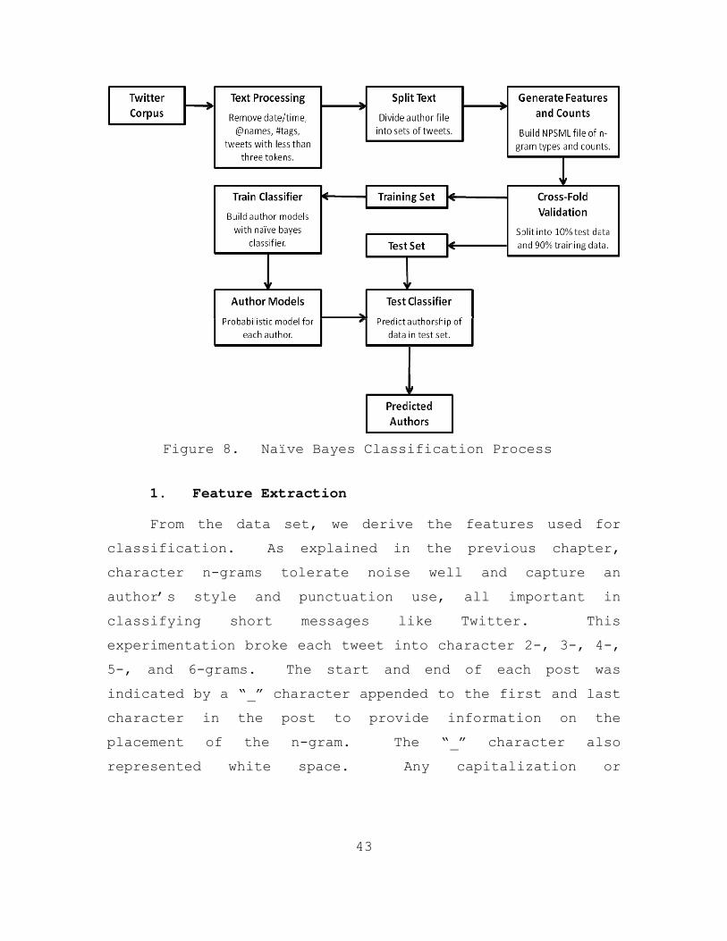
43
Figure 8. Naïve Bayes Classification Process
1. Feature Extraction
From the data set, we derive the features used for
classification. As explained in the previous chapter,
character n-grams tolerate noise well and capture an
author’s style and punctuation use, all important in
classifying short messages like Twitter. This
experimentation broke each tweet into character 2-, 3-, 4-,
5-, and 6-grams. The start and end of each post was
indicated by a “_” character appended to the first and last
character in the post to provide information on the
placement of the n-gram. The “_” character also
represented white space. Any capitalization or
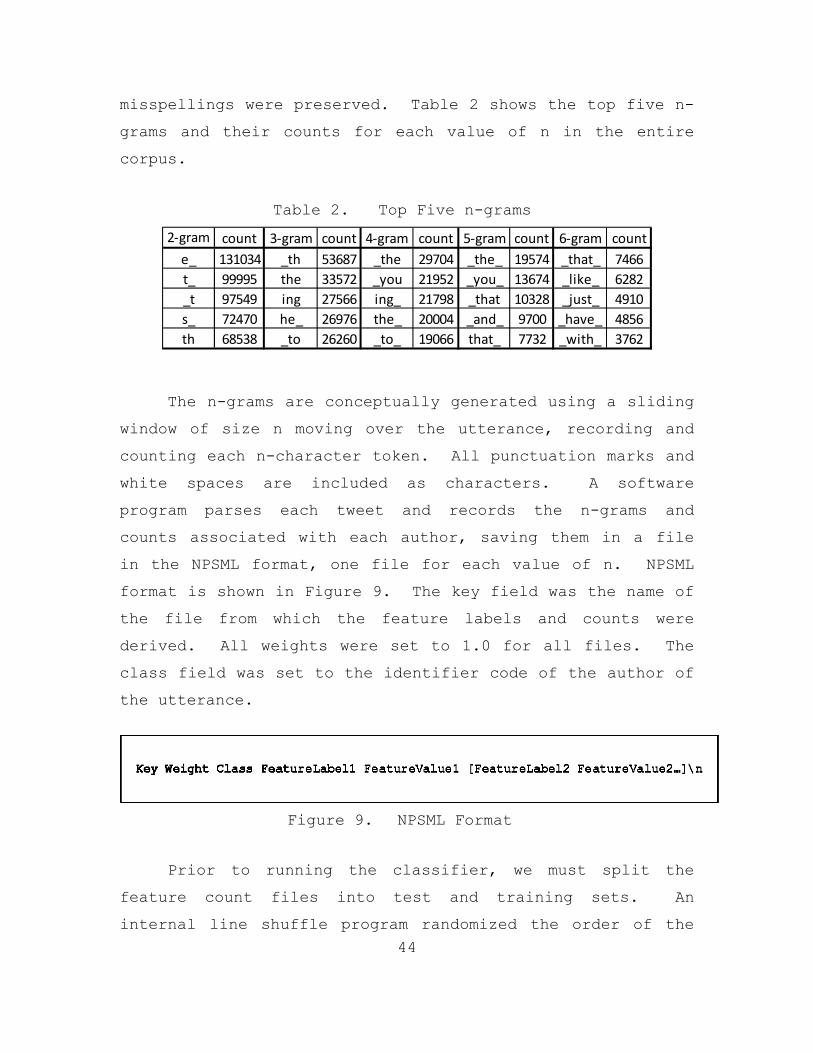
44
misspellings were preserved. Table 2 shows the top five n-
grams and their counts for each value of n in the entire
corpus.
Table 2. Top Five n-grams
2‐gram count 3‐gram count 4‐gram count 5‐gram count 6‐gram counte_ 131034 _th 53687 _the 29704 _the_ 19574 _that_ 7466t_ 99995 the 33572 _you 21952 _you_ 13674 _like_ 6282_t 97549 ing 27566 ing_ 21798 _that 10328 _just_ 4910s_ 72470 he_ 26976 the_ 20004 _and_ 9700 _have_ 4856th 68538 _to 26260 _to_ 19066 that_ 7732 _with_ 3762
The n-grams are conceptually generated using a sliding
window of size n moving over the utterance, recording and
counting each n-character token. All punctuation marks and
white spaces are included as characters. A software
program parses each tweet and records the n-grams and
counts associated with each author, saving them in a file
in the NPSML format, one file for each value of n. NPSML
format is shown in Figure 9. The key field was the name of
the file from which the feature labels and counts were
derived. All weights were set to 1.0 for all files. The
class field was set to the identifier code of the author of
the utterance.
Figure 9. NPSML Format
Prior to running the classifier, we must split the
feature count files into test and training sets. An
internal line shuffle program randomized the order of the

45
posts in the feature count files. A ten-fold cross
validation was applied, in which a feature count file was
split into ten subfiles, with nine used for training the
classifier and one used for testing it. The nps-bTTSplit
software program from the NPS Machine Learning Library [32]
was used to generate the test and train files, ensuring
each author was represented with an equal number of posts
in each of the subfiles. None of the posts used in a
training file were also used in the associated test file.
2. Naïve Bayes Classifier
This experimentation used the Naval Postgraduate
School Natural Language Processing Lab naïve Bayes
classification package. This software package uses the
NPSML file format as input. The learning portion uses the
smoothed feature counts from the input training data file
to generate a probabilistic model. One set of experiments
was conducted using Laplace add-one smoothing. A second
set was conducted using Witten-Bell smoothing. The
classification program used the model generated by the
learning program and the NPSML-formatted test data to
determine the most probable class assignment for each test
utterance. The program output the key and predicted class
for each utterance in the test file. Each fold of the 10-
fold cross validation was run and the outputs averaged for
the final classification result. As each author has an
equal number of tweets in the data set, prior probabilities
for each author were fixed and equal.

46
D. PATTERN OF LIFE ANALYSIS
Human beings often fall into habitual daily routines.
The act of communicating with others may fit into this
routine, allowing an observer to discern a pattern. A user
may log into his computer at the same time every weekday
morning, or call his mother to chat during his commute home
every evening. Analyzing a user’s communication patterns
may aid in the identification of the user.
1. Twitter Time Analysis
Each tweet collected includes a date/time field.
Figure 10 shows the format of the date/time field. This
analysis focused on a simple pattern analysis of send time
by hour of the day. This may capture any user patterns
centered on a work or school schedule.
Figure 10. Date/Time Field Format
The date/time fields were stripped from each tweet and
saved in a separate file for each user. A line-by-line
shuffle program randomized the order of the timestamps.
The first 120 were taken from each author file as a sample
set. This sample set was then subdivided, grouping
timestamps into files labeled with the author as the class.
We used training set sizes of three, five, ten, and twelve

47
for testing. The files were processed into the NPSML
format with the sent hours and their counts as the keys and
values contained in each file. The NPSML files were
processed in the same manner as the text files. The hours
and counts were divided into test and training groups,
holding out 10% as a test set. The naïve Bayes learning
and classify programs were run on a 10-fold cross
validation using Witten-Bell smoothing and the results
averaged to determine the final output class for each test
input. Other experiments were conducted with varying
timestamp quantities and training set sizes, which are
explained in the Results section of this thesis.
2. Social Network Analysis
Another characteristic of an individual’s
communication patterns is the group of people with whom he
communicates. In a telephone or SMS network, discerning
this would require some access to signaling information or
service provider records. In Twitter, users often include
the screen name of the user they are specifically speaking
to or about in their tweet. Layton et al. noted a 26%
reduction in the accuracy of their authorship attribution
method when screen names were removed from the tweets. For
a simple social network analysis, we examined the screen
names referenced by the users in our corpus independent of
the text of their tweets.
The data processing used to conduct the social network
analysis was identical to the date analysis. Instead of
pulling the date/time field out of each tweet, any @name
found in parsing was saved to a file by author. The
shuffling, splitting, and grouping into training sets was

48
conducted using sets of three, six, ten, and twelve out of
120 @names per author. NPSML files of @names and their
counts per author were built. These were divided into test
and train sets, and naïve Bayes learning and classification
with Witten-Bell smoothing was performed on a 10-fold cross
validation with the results averaged to give final output
classes for each input.
E. CELL PHONE SIGNAL ANALYSIS
Based on the success of [4], we focused on signal
modulation features to build device characteristic vectors.
GSM modulation parameters are governed by the European
Telecommunications Standards Institute (ETSI) in their 3rd
Generation Partnership Project (3GPP) standards [33], [34].
Cell phone manufacturers test their products for quality
assurance purposes, ensuring phone users have an acceptable
link quality and that phones do not interfere with other
users. Three signal characteristics that are measured and
controlled are peak phase error, root mean square (RMS)
phase error, and frequency error. The Agilent 8922S GSM
Test Set is a signal analyzer geared for measuring these
standard modulation characteristics of a GSM mobile
station.
1. Signal Collection
The equipment used in conducting the mobile station
signal measurements was the Agilent 8922S GSM Test Set, the
LGS Innovations Tactical Base Station Router (TacBSR), and
an assortment of unlocked GSM-capable cell phones. The
8922S was run in test mode with small whip antenna serving
as the RF input element. The use of an antenna required

49
adjustment of the expected input amplitude decibel value.
This varied by phone and was set based on Test Set
measurements of the phone output power and the presence or
absence of RF overload errors. Figure 11 shows the cell
control screen where these values were set.
Figure 11. Cell Control Screen (From [35])
In test mode, the 8922S transmits a GSM broadcast
signal on a specified frequency channel, or absolute radio
frequency channel number (ARFCN). It has a separate ARFCN
designated for the traffic channel the phone will use to
communicate with the BTS. Our phones could not connect to
the 8922S as a BTS with the antenna and SIM cards we had
available for use, so we used the TacBSR as the BTS. The
TacBSR was configured to operate in the E-GSM900 spectrum
using ARFCN 875 as the traffic channel. This correlates to
an uplink frequency of 882.2 MHz. The 8922S was configured
as a midpoint collector listening to ARFCN 875. All the
phones we tested operated in this GSM band.

50
Besides the amplitude of the input, two other settings
required adjustment before taking measurements, the traffic
channel timeslot and the trigger delay. When setting up a
call with the TacBSR, we noted the calling phone was
assigned timeslot 2 and the called phone was assigned
timeslot 3. To establish a traffic channel for
measurement, we had to establish a voice call between two
phones. The calling phone was noted and proper traffic
channels were set when conducting measurements. The
trigger delay sets the time delay between a valid trigger
event and the beginning of a measurement. The 8922S uses
the midamble of a GSM frame as a trigger, as it is easy to
detect. The Data Bits screen of the Phase/Frequency page
shows the bit sequence of the GSM frame, highlighting the
midamble. Figure 12 shows an example of this screen. The
trigger timing was set by observing the value of the First
Bit field and adjusting the trigger delay to force that
value close to zero.
Figure 12. Data Bits Screen (From [35])

51
Once the amplitude, timeslot, and trigger delay were
set, we measured the three modulation characteristics. A
more detailed explanation of the modulation measurements is
included in Appendix A. This was done from the
Phase/Frequency page, shown in Figure 13. To get an
average value over a fixed number of transmission bursts
for each measurement, we used the multi-burst feature for
ten bursts. The measured phone was held near the antenna
of the 8922S, while the phone on the other end of the call
was placed across the room to minimize cross-channel
interference. We collected 30 values for peak phase, RMS
phase, and frequency error as averaged over 10 transmission
bursts. The values were read from the screen and recorded.
Figure 13. Phase and Frequency Error Screen (Multi-
burst on)(From [35])

52
The data collection method for the cell phone features
was sufficiently time and labor intensive that we used the
30 data samples of each feature from each phone as the
foundation for building a larger data set. The measured
values of each feature were input into a program that built
a probability density function based on a histogram of the
results. The program smoothed the samples by building a
histogram, and then used the scipy gaussian_kde module to
create the probability density function. It then drew a
specified number of random values weighted by the
probability density [36]. We used this method to generate
160 more values representative of each handset.
2. Data Analysis and Classification
The modulation characteristic data required some
preprocessing before use as an identification vector. An
average and standard deviation value was calculated for
each characteristic for each phone. The smallest standard
deviation value of each feature was used as a bin size, and
the raw data was binned, generating histograms for each
phone. For example, if the standard deviation of the
frequency error for phone 1 was 8.2, phone 2 was 9.5, and
phone 3 was 7.3, the bin size for frequency error for the
three phones would be 7.3. Binning the data reduced noise
from the measurement process and discretized values from
continuous domains to aid in feature counting for the
classification step. Each set of {peak phase error, RMS
phase error, frequency error} bin values for each
collection data point served as a feature vector for the
phone it was associated with.

53
For learning and classification, the feature vectors
were split into separate files. As with the time and name
analysis, we experimented with varying the size of the
training set. A software program turned each set of files
into an NPSML-formatted file of features and their counts.
The NPSML files were provided as input to the NPS naive
Bayes learning and classifying programs. The average
results of a 10-fold cross validation were given as the
output classes. We conducted experiments with varying
numbers of feature vectors and document sizes, which are
explained further in the next chapter of this thesis.
F. COMBINING CLASSIFIERS
Once the individual classification results were
obtained, we experimented with combining these results to
see if there was any subsequent improvement in accuracy.
The NPS nb-classify program can provide as its output the
logarithms of the probabilities for each class label.
Based on the availability of that information and the prior
work described in the previous chapter, we chose the sum
rule combination scheme. The sum rule takes the
probability outputs of a set of classifiers and adds the
probability values of each class label. The class label
with the maximum summed value is selected as the output
label.
In the first set of experiments, one phone was
assigned to one author. The output probability logarithms
for each class label from the phone classifier were added
to the output probability logarithms of the text
classifier. The maximum combined value of each
classification test was taken as the result. We conducted

54
20 experiments rotating the author assignment for each
phone to verify the consistency of results across phone-
author pairings. The accuracy results for each pairing
were averaged to obtain the overall accuracy. Appendix E
contains the phone-author pairing matrix.
To mitigate the influence of the differences in
magnitudes of the text and device probability logarithms on
the summation result, these values were normalized across
the individual classes for each classifier output. The
normalized output of the signal classifier for a particular
phone was added to the normalized output of the text
classifier for its associated author. The experimentation
process was repeated on these values. The pattern of life
classifier results were included in another set of
experiments, adding the output values to the text and
device output values to attain a combined output value.
Another experiment was conducted to gauge the
effectiveness of the combined classifier at detecting a
change of author on a single phone. Using the same set of
20 authors and phones as above, the tweet text set was
modified to simulate a change of author. We chose two of
the 20 authors to swap. Out of the 50 tweet per author
data set, 10 tweets from each of the two authors were
labeled as the other author. The labeling scheme included
a flag so that we could identify the modified tweets after
classification. The modified test set was classified using
the classifier model trained previously. None of the
tweets in the test data had been part of the training
model. The results were normalized and added to the
normalized phone classifier results. The results of the
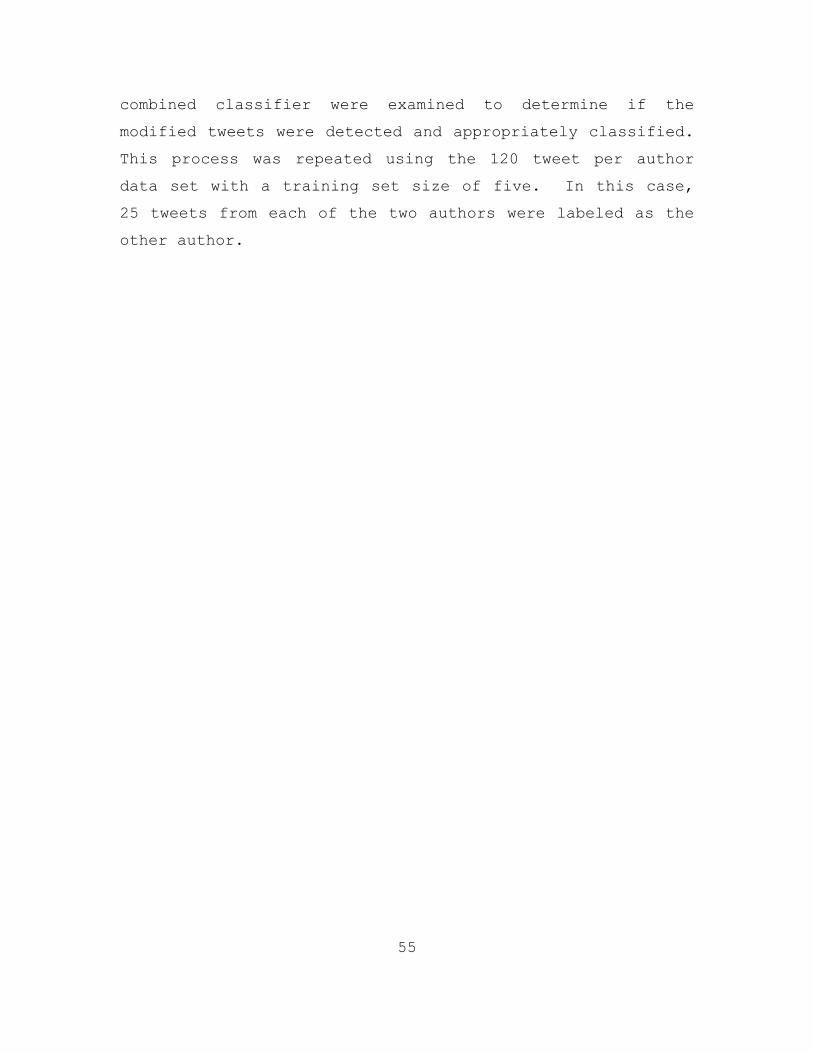
55
combined classifier were examined to determine if the
modified tweets were detected and appropriately classified.
This process was repeated using the 120 tweet per author
data set with a training set size of five. In this case,
25 tweets from each of the two authors were labeled as the
other author.

56
THIS PAGE INTENTIONALLY LEFT BLANK

57
IV. RESULTS AND ANALYSIS
A. TEXT RESULTS
This section examines the authorship attribution
results from classification of the Twitter text corpus. We
first present the effects of varying the size of the
character n-gram in the feature set and the type of
smoothing used. As 140 characters or less do not contain
much feature information to make a profile, we experiment
with combining several individual tweets from one author
into a “document”, increasing the total word count of the
experimental unit of analysis by using a set of multiple
tweets rather than just one tweet, then training the
classifier and testing with these “documents”. We
experiment with classifying data sets consisting of
different total quantities of tweets per author, combining
these tweets into documents of varying tweet count. We
then test the effect on classifier accuracy of changing the
number of authors and the total number of tweets per author
in the data set.
Analysis of the Twitter text showed that the author
could be determined by a naïve Bayes classifier at a rate
significantly better than chance. Table 3 shows the
accuracy results averaged over a ten-fold cross validation
of a multiclass classification of 50 authors using 230
tweets per author with character 2- through 6-grams as the
feature set. Results for LaPlace add-one and Witten-Bell
smoothing are presented. These smoothing techniques are

58
explained in more detail in Chapter II, Section F. As
expected, the Witten-Bell smoothing performed better than
the add-one smoothing.
Table 3. Classification Accuracy Results for 50 Authors With 230 Tweets Per Author
LaPlace Witten‐Bell2‐gram 0.369 0.4073‐gram 0.412 0.4954‐gram 0.427 0.4935‐gram 0.420 0.4586‐gram 0.389 0.415
Smoothing
In order to compare our results to those published in
[3], we performed the same analysis using 120 tweets per
author. The SCAP method shows better results than our
classifier. Table 4 shows our accuracy results compared to
their results when their @name and #tag removal
preprocessor is applied.
Table 4. Classification Accuracy Results for 50 Authors With 120 Tweets Per Author With Comparison to SCAP
Method
LaPlace Witten‐Bell SCAP [3]2‐gram 0.300 0.349 0.3573‐gram 0.326 0.403 0.5274‐gram 0.327 0.375 0.5445‐gram 0.313 0.334 0.5366‐gram 0.287 0.299 0.512
Smoothing
The results presented thus far use a single tweet as a
document for classification purposes. Combining multiple

59
tweets in a document and using a set of these documents to
build the feature and count values for the training and
test inputs to the classifier improves the accuracy results
significantly. Table 5 shows the accuracy results of the
classifier averaged over the ten-fold cross validation for
50 authors with 230 total tweets per author divided into
ten documents of 23 tweets each, a value determined
empirically to provide the best accuracy results as
described next.
Table 5. Classification Accuracy Results for 50 Authors With 230 Tweets per Author Combined into Documents
of Size 23 Tweets
LaPlace Witten‐Bell2‐gram 0.915 0.9773‐gram 0.811 0.9964‐gram 0.849 0.9965‐gram 0.913 0.9946‐gram 0.947 0.992
Smoothing
Grouping multiple tweets into a document improves the
accuracy of the classifier significantly. As the character
3-gram feature and Witten-Bell smoothing process provided
the best results in early testing, we continued further
testing with those parameters fixed. The next set of tests
evaluated the effects of document size, in tweets, on
accuracy. To complete the 90%:10% train to test split, a
minimum of ten documents are required for classification.
We used ten documents with a range of five to 20 tweets per
document. Table 6 shows the results of that experiment.

60
Table 6. Classification Accuracy Results for 50 Authors Using 10 Documents With Increasing Number of
Tweets per Document
document size
total # tweets accuracy
5 50 0.55410 100 0.88215 150 0.9720 200 0.99
Fixing the previous experiment at ten documents caused
the larger document sizes to use a proportionally larger
total number of tweets for classification. To determine
whether the accuracy improvement could be attributed to the
document size or the total number of tweets in the data
set, we conducted another experiment in which we set the
total number of tweets at or near 150. In a situation
where the available number of messages per author is
limited, this distinction is important in designing an
accurate classification process. If the use of multi-tweet
documents enhances classifier accuracy in a fixed corpus
size, acceptable results may be obtained using fewer tweets
per author than if tweets are tested individually. The
document size was varied from five to 15 tweets per
document. The total number of tweets per classification
run was the multiple of the document size closest to 150.
Figure 14 shows the results of this experiment. The
document size range from one to five tweets was examined
further, finding the classification accuracy for 50, 100,
and 150 tweets across that range. Those results are
displayed in Figure 15.

61
Figure 14. Classification Accuracy for 50 Authors Using 150 Tweets per Author With Increasing Document
Size
Figure 15. Classification Accuracy for 50 Authors by
Document Size and Total Number of Tweets per Author

62
The effects of changing the number of tweets per
author and changing the number of authors were evaluated in
more detail. The number of authors in each trial was
varied from two to 50, selected randomly from the set of 50
authors. The number of tweets was varied from 30 to 190
with a document size of one tweet. Figures 16 and 17 show
graphs of the accuracy results over the range examined.
Improvement in accuracy appears to level off at about 22
authors.
Figure 16. Classification Accuracy Results for Various
Total Tweet Values Per Author With Increasing Author Count

63
Figure 17. Classification Accuracy Results for Various
Author Counts With Increasing Total Tweet Per Author Values
The classification accuracy curve for increasing
number of authors in the data set levels out at 20 authors.
We conducted further experimentation with a set of 20
authors randomly selected from the 50-author data set. We
used total tweet per author values of 30, 50, 100, 120, and
150. The document sizes tested ranged from one to 15
tweets per document. Figures 18 and 19 show the classifier

64
accuracy results averaged over a ten-fold cross validation
for 20 authors with varying numbers of tweets per author
and tweets per document.
Figure 18. Classification Results for 20 Authors With
Varying Values of Tweets per Author and Tweets per Document

65
Figure 19. Classification Results for 20 Authors With
More Than 100 Tweets per Author and Varying Tweets per Document
We next investigated if the improvement in
classification accuracy results generated by combining
multiple tweets into a document occurred during the
training or the testing of the classifier. Using the set
of 20 authors, we took the models built for 50 tweets per
author with five tweets per document, 100 tweets per author
with five and ten tweets per document, and 120 tweets per
author with five and 12 tweets per document and tested a
new set of single tweets of the appropriate size on each
model. The results of these tests are presented in Table
7. The consistency of the accuracy results implies the
added feature depth of the multi-tweet document generates
its accuracy benefits during the testing of the classifier
rather than the training.

66
Table 7. Classification Accuracy Results for Single Tweet Documents Tested on Models Trained on Multi-Tweet
Documents of the Specified Quantity
Tweets per Author
Document Size Trained On
Accuracy
50 1 0.33550 5 0.335100 1 0.417100 5 0.421100 10 0.4275120 1 0.4496120 5 0.4554120 12 0.4471
This section presented the results of a series of
classification experiments conducted on a Twitter corpus of
50 authors. We found that using character 3-grams as a
feature set and Witten-Bell smoothing produced the best
accuracy results. Classification accuracy improved as the
number of tweets per author increased, reaching 49.5%
accuracy at 230 tweets per author, a value based on the
smallest author data set in the corpus. Increasing the
feature depth of the text by combining multiple tweets into
a document and training and testing the classifier with the
multi-tweet documents improves classification accuracy
significantly, with accuracy levels reaching 90% at ten
tweets per document for 120 and 150 tweets per author and
99% at 23 tweets per document for 230 tweets per author.
Confusion matrices and per-author accuracy results for the
above tests are provided in Appendix B.

67
B. PATTERN OF LIFE RESULTS
The pattern of life analysis builds a basic
description of an author’s tweeting habits by examining the
time of day he sends his messages. We use the hour of day
the message is sent as the feature used for classification.
Like in the text classification process, we try to increase
the depth of the feature set by combining the send times of
multiple tweets into one training set and using the
<feature, count> values of the combined set as the input to
the classifier.
Analysis of the hour of day the users tweet showed
that the author of a tweet could be determined by a naïve
Bayes classifier at an accuracy rate just slightly better
than chance. We used the send hour (GMT) of 120 tweets for
each author as the time value. As the send time is
reported in hour:minute:second format, this serves to bin
the times into 24 bins, one per hour. The 120-hour values
were split into training sets, similar to grouping multiple
tweets into documents as in the previous section. We
experimented with training set sizes ranging from one to 12
tweet hours per set. As with the message text, accuracy
improved when grouping multiple tweet times into a training
set. The training sets are input into the naïve Bayes
classifier and trained and tested using Witten-Bell
smoothing. Figure 20 shows the classification accuracy
results averaged over a ten-fold cross validation for 50
authors with 120 tweet time values per author grouped into
training sets ranging in size from one to 12 tweet time
values per set.

68
Figure 20. Classification Accuracy for 50 Authors of
120 Tweet Times per Author With Increasing Number of Tweet Times per Training Set
Compared to the text classification results, time of
day was not an effective way to discriminate between
authors. As the testing focused on English speakers, it is
possible that many of the users were located in similar
time zones, and thus maintained similar schedules. A few
authors could be classified with very good results, with
two authors identified at over 60% accuracy over 120 tweets
with a training set size of three. Table 8 shows the
accuracy result for each author for 120 tweets per author
and training set sizes of three, five, ten, and 12 tweet
hours per set. Histograms of the tweet send times for each
author are presented in Appendix C.

69
Table 8. Classifier Accuracy Results for Each Author Using 120 Tweet Times per Author and Increasing Number
of Tweet Times per Training Set
Author 3 5 10 12 Author 3 5 10 120785 0.0000 0.0833 0.0833 0.2000 5599 0.0500 0.1667 0.4167 0.40000806 0.1000 0.1250 0.4167 0.5000 5698 0.3500 0.3750 0.8333 0.60001045 0.1500 0.2083 0.2500 0.5000 5742 0.3000 0.3750 0.4167 0.50001388 0.0000 0.0833 0.0833 0.2000 6111 0.0250 0.0417 0.0000 0.30001734 0.1500 0.1250 0.3333 0.4000 6172 0.1000 0.1250 0.2500 0.20001921 0.2000 0.1250 0.3333 0.3000 6705 0.2500 0.2500 0.4167 0.60001931 0.2500 0.2500 0.3333 0.4000 6886 0.0250 0.1250 0.2500 0.20002241 0.1250 0.3333 0.3333 0.2000 7100 0.0250 0.0000 0.0000 0.00002319 0.0250 0.0417 0.0000 0.1000 7106 0.0750 0.2500 0.4167 0.40002546 0.1250 0.1250 0.2500 0.3000 7227 0.6250 0.8333 0.9167 1.00002622 0.2000 0.3333 0.3333 0.5000 7241 0.1250 0.1667 0.1667 0.00002691 0.0000 0.0000 0.0000 0.0000 7457 0.1750 0.2500 0.4167 0.40002744 0.1000 0.2917 0.4167 0.5000 7541 0.0250 0.0833 0.0833 0.10002753 0.0000 0.0417 0.0000 0.0000 7754 0.0750 0.1667 0.1667 0.40003155 0.3750 0.4583 0.7500 0.8000 7958 0.0750 0.0833 0.3333 0.20003204 0.0500 0.1250 0.2500 0.2000 8164 0.1000 0.2500 0.5000 0.30003281 0.6000 0.3750 0.5833 0.8000 8181 0.0500 0.0833 0.0000 0.30003317 0.1250 0.1250 0.1667 0.4000 8487 0.0000 0.0417 0.0000 0.20003565 0.1750 0.1667 0.4167 0.4000 8632 0.0250 0.0833 0.1667 0.10003693 0.4500 0.4167 0.6667 0.7000 8700 0.0250 0.0833 0.0000 0.00003824 0.6250 0.7500 0.9167 0.9000 8832 0.0500 0.1667 0.0833 0.30003883 0.0250 0.1667 0.1667 0.3000 8846 0.2250 0.1667 0.5000 0.50004045 0.0250 0.0000 0.0833 0.1000 9235 0.1750 0.2083 0.5000 0.50004117 0.1000 0.1667 0.2500 0.3000 9417 0.3250 0.2500 0.5000 0.30004133 0.2750 0.2083 0.7500 0.7000 9716 0.0250 0.0417 0.0833 0.00004431 0.1250 0.1667 0.1667 0.3000 9800 0.0000 0.0833 0.3333 0.10005106 0.2000 0.2500 0.3333 0.4000
Tweet Hours per Training Set Tweet Hours per Training Set
C. SOCIAL NETWORK RESULTS
Analysis of the social network of the authors as
determined by the @names referenced in their tweets
provided excellent accuracy results. The corpus contained
a total of 72,888 references to 6,105 unique @names. The
least connected author, gauged by the author’s ratio of
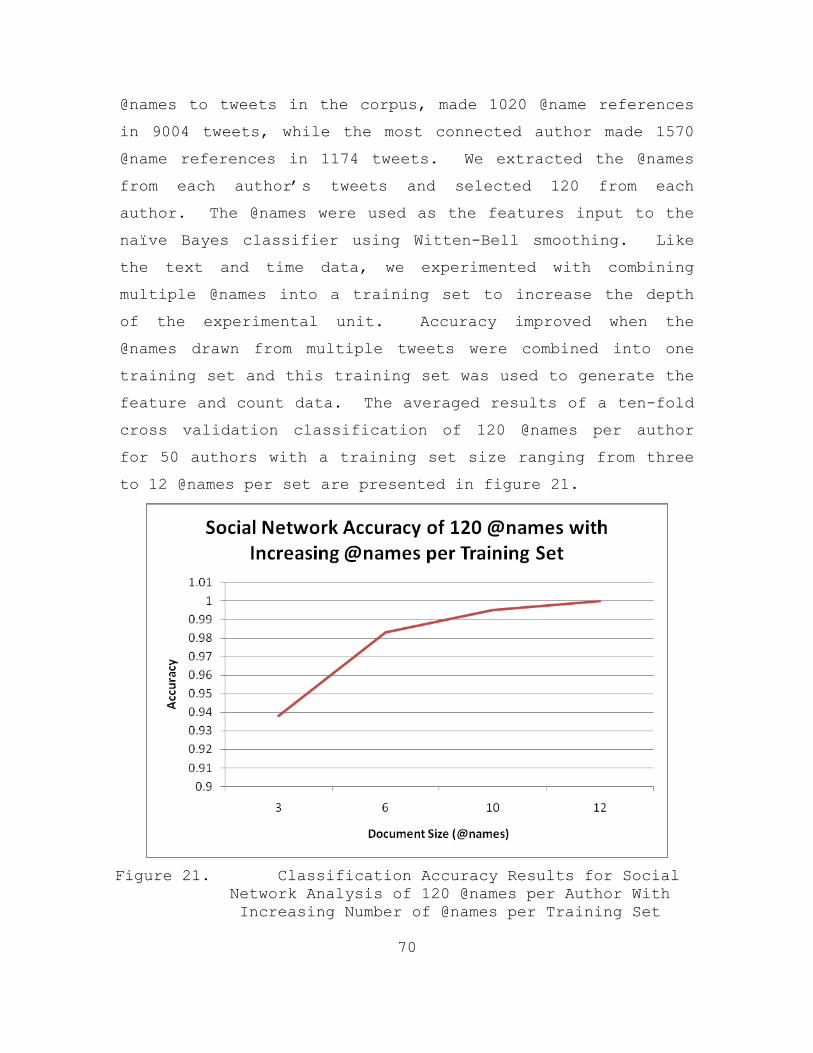
70
@names to tweets in the corpus, made 1020 @name references
in 9004 tweets, while the most connected author made 1570
@name references in 1174 tweets. We extracted the @names
from each author’s tweets and selected 120 from each
author. The @names were used as the features input to the
naïve Bayes classifier using Witten-Bell smoothing. Like
the text and time data, we experimented with combining
multiple @names into a training set to increase the depth
of the experimental unit. Accuracy improved when the
@names drawn from multiple tweets were combined into one
training set and this training set was used to generate the
feature and count data. The averaged results of a ten-fold
cross validation classification of 120 @names per author
for 50 authors with a training set size ranging from three
to 12 @names per set are presented in figure 21.
Figure 21. Classification Accuracy Results for Social
Network Analysis of 120 @names per Author With Increasing Number of @names per Training Set
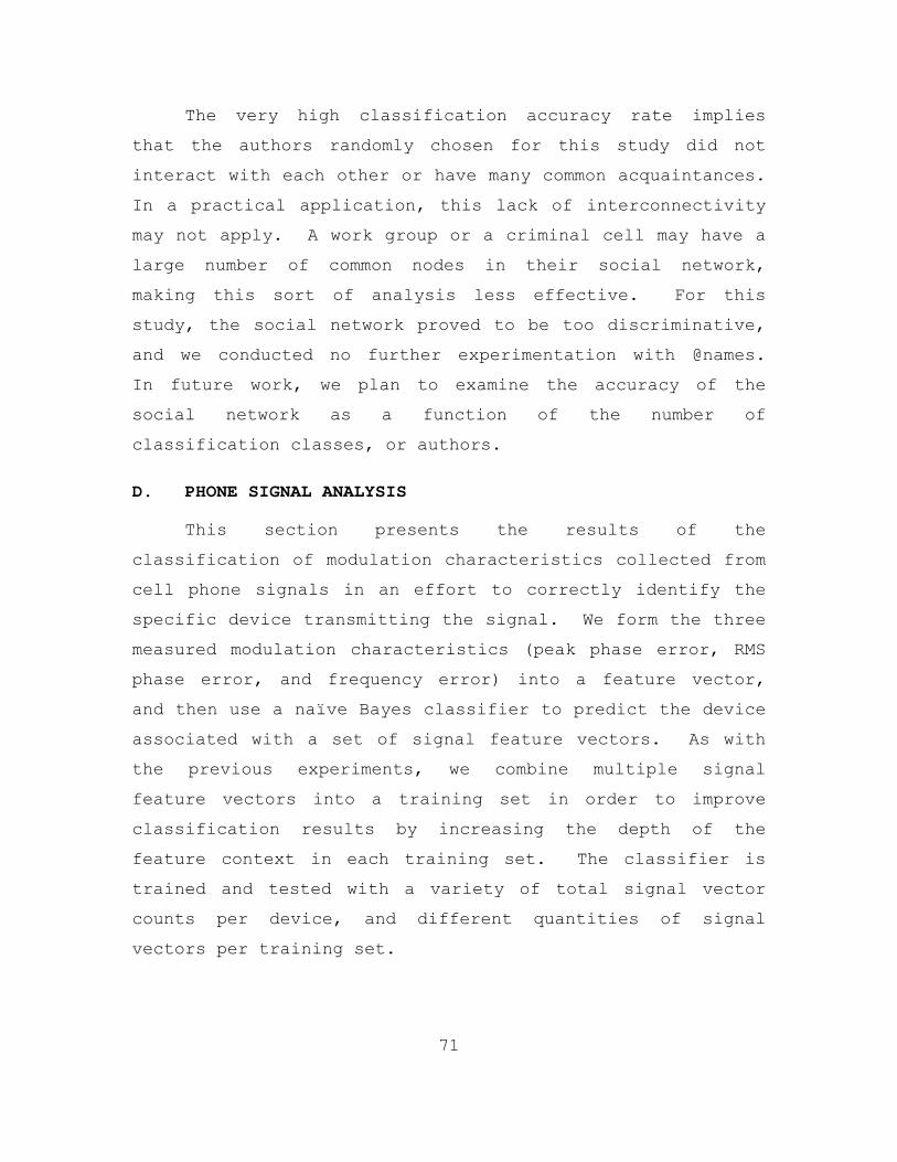
71
The very high classification accuracy rate implies
that the authors randomly chosen for this study did not
interact with each other or have many common acquaintances.
In a practical application, this lack of interconnectivity
may not apply. A work group or a criminal cell may have a
large number of common nodes in their social network,
making this sort of analysis less effective. For this
study, the social network proved to be too discriminative,
and we conducted no further experimentation with @names.
In future work, we plan to examine the accuracy of the
social network as a function of the number of
classification classes, or authors.
D. PHONE SIGNAL ANALYSIS
This section presents the results of the
classification of modulation characteristics collected from
cell phone signals in an effort to correctly identify the
specific device transmitting the signal. We form the three
measured modulation characteristics (peak phase error, RMS
phase error, and frequency error) into a feature vector,
and then use a naïve Bayes classifier to predict the device
associated with a set of signal feature vectors. As with
the previous experiments, we combine multiple signal
feature vectors into a training set in order to improve
classification results by increasing the depth of the
feature context in each training set. The classifier is
trained and tested with a variety of total signal vector
counts per device, and different quantities of signal
vectors per training set.

72
Analysis of the phone signal modulation
characteristics showed that devices could be identified by
the naïve Bayes classifier at an accuracy level well above
random chance. Figure 22 shows the accuracy results
averaged over a ten-fold cross validation for 20 phones
with a total signal feature vector quantity of 30 – 150
vectors per device and a training set size of one to five
vectors per training set.
Figure 22. Classification Accuracy for 20 Devices With
Varying Vectors per Training Set and Total Vectors per Device
Training set sizes larger than five vectors per set
were explored using 150 total data vectors. Figure 23
shows the results of these experiments for 20 phones. As
the training set size increases the total number of
classification results per phone decreases, giving each
incorrect classification a larger impact on the accuracy

73
result. For example, 150 data vectors divided into five
per training set gives 30 sets for classification.
Incorrectly classifying one of these documents yields a
96.7% accuracy result. When 150 data vectors are grouped
into training sets of size 15, ten sets are created for
classification. Incorrectly classifying one set yields a
90% accuracy result. Figure 23 reflects this phenomenon.
Figure 23. Classification Accuracy Results for 20
Phones With 150 Data Vectors and Varying Document Size
Confusion matrices and accuracy results per phone are
included in Appendix D. In future work, we wish to
investigate which features of the phone signals provide the
most discriminatory classification power.
E. COMBINED CLASSIFIERS
Combining the outputs of the individual classifiers
improved upon the authorship attribution results of the

74
individual text classifier. Per the sum-rule combination
scheme discussed in Chapter II, our experimentation added
the output probability logarithms, averaged over a ten-fold
cross validation, of the individual phone and text
classifiers. The text data sets used in the experiments
were the classification results from the 20 authors using
30, 50, 100, 120, and 150 tweets per author and document
sizes of one to 15 tweets per document. The phone data
sets used were the classification results from 20 phones
using the same number of signal vectors per phone and
signal vectors per training set as the text data sets. We
repeated this process for selected data sets after
normalizing the output probability logarithms. Figures 24-
28 show the accuracy results of the individual and combined
classifiers for the five data sets. Appendix E contains
the accuracy results for each author-phone pairing tested.
Figure 24. Classification Accuracy of Individual and
Combined Classifiers for 30 Tweets/Signal Vectors and Various Training Set Sizes

75
Figure 25. Classification Accuracy of Individual and
Combined Classifiers for 50 Tweets/Signal Vectors and Various Training Set Sizes
Figure 26. Classification Accuracy of Individual and
Combined Classifiers for 100 Tweets/Signal Vectors and Various Training Set Sizes

76
Figure 27. Classification Accuracy of Individual and
Combined Classifiers for 120 Tweets/Signal Vectors and Various Training Set Sizes
Figure 28. Classification Accuracy of Individual and
Combined Classifiers for 150 Tweets/Signal Vectors and Various Training Set Sizes

77
Normalizing the output probability logarithms, before
adding them together, results in accuracy values superior
to either of the individual classifiers. The probability
logarithm outputs of the text classifier are orders of
magnitude smaller than the phone classifier, with bigger
variance between the label values because of the much
larger text feature space. Table 9 shows an example using
the author 2744 and the phone htc376.
Table 9. Comparing Combination of Probability Logarithms and Combination of Normalized Probability
Logarithms
probability logarithms normalizedhtc376 2744 sum htc376 2744 sum
bberry 1045 ‐58.390 ‐1536.188 ‐1594.578 ‐0.0579 ‐0.0498 ‐0.1077htc371 1388 ‐55.380 ‐1481.225 ‐1536.605 ‐0.0550 ‐0.0480 ‐0.1030htc373 1734 ‐48.555 ‐1573.074 ‐1621.629 ‐0.0482 ‐0.0510 ‐0.0992htc374 1921 ‐32.916 ‐1524.800 ‐1557.716 ‐0.0327 ‐0.0494 ‐0.0821htc375 2546 ‐47.781 ‐1530.894 ‐1578.675 ‐0.0474 ‐0.0496 ‐0.0970htc376 2744 ‐30.337 ‐1515.917 ‐1546.253 ‐0.0301 ‐0.0491 ‐0.0792htc601 3155 ‐47.069 ‐1527.684 ‐1574.753 ‐0.0467 ‐0.0495 ‐0.0962htc_rob 3693 ‐47.608 ‐1603.219 ‐1650.828 ‐0.0472 ‐0.0520 ‐0.0992iphone4 5599 ‐53.588 ‐1522.475 ‐1576.063 ‐0.0532 ‐0.0493 ‐0.1025iphone5 5742 ‐51.262 ‐1548.413 ‐1599.674 ‐0.0509 ‐0.0502 ‐0.1011iphone7 6111 ‐50.704 ‐1567.741 ‐1618.446 ‐0.0503 ‐0.0508 ‐0.1011n8_594 6886 ‐56.335 ‐1545.237 ‐1601.572 ‐0.0559 ‐0.0501 ‐0.1060n97_430 7100 ‐54.006 ‐1542.504 ‐1596.511 ‐0.0536 ‐0.0500 ‐0.1036n97_444 7241 ‐56.450 ‐1570.351 ‐1626.801 ‐0.0560 ‐0.0509 ‐0.1069n97_618 7754 ‐56.529 ‐1496.549 ‐1553.078 ‐0.0561 ‐0.0485 ‐0.1046n97_620 7958 ‐54.762 ‐1523.541 ‐1578.304 ‐0.0543 ‐0.0494 ‐0.1037nok_128 8164 ‐51.402 ‐1600.487 ‐1651.889 ‐0.0510 ‐0.0519 ‐0.1029nok_e5 8487 ‐60.139 ‐1554.265 ‐1614.404 ‐0.0597 ‐0.0504 ‐0.1101nok_e62 9417 ‐49.989 ‐1543.362 ‐1593.351 ‐0.0496 ‐0.0500 ‐0.0996treo 9800 ‐44.480 ‐1546.871 ‐1591.351 ‐0.0441 ‐0.0501 ‐0.0943
Max ‐30.337 ‐1481.225 ‐1536.605 ‐0.0301 ‐0.0480 ‐0.0792
78
The text classifier incorrectly selects author 1388 as
the most probable class, with a probability logarithm
output 34.691 orders of magnitude higher than the actual
class. The phone classifier correctly selects htc376, but
its probability logarithm output is only 25.043 orders of
magnitude more than htc371, the phone associated with
author 1388. Thus, the combined classifier selects the
htc371-1388 pair. Once the probability logarithms are
normalized, the relative variation between class labels
decreases. The text classifier selection of 1388 is only
0.0011 orders of magnitude greater than the value for 2744,
while the value of htc371 is now 0.0249 orders of magnitude
less than the correct value of htc376. Thus, the combined
classifier outputs the correct htc376-2744 pairing based on
the strength of the phone classifier.
Another example using the same phone-author pair
demonstrates how the normalized probability logarithms can
have a negative effect on the combined classifier accuracy.
Table 10 shows a set of classifier outputs in which the
incorrect phone classifier causes the normalized
probability logarithm combination to make an incorrect
phone-author pair classification, while the non-normalized
output combination selected the correct pair.

79
Table 10. Normalized Probability Logarithm Combination Resulting in Incorrect Classification
probability logarithms normalizedhtc376 2744 sum htc376 2744 sum
bberry 1045 ‐61.569 ‐1889.374 ‐1950.943 ‐0.0576 ‐0.0501 ‐0.1077htc371 1388 ‐59.819 ‐1835.965 ‐1895.783 ‐0.0560 ‐0.0487 ‐0.1047htc373 1734 ‐57.650 ‐1886.810 ‐1944.460 ‐0.0540 ‐0.0500 ‐0.1040htc374 1921 ‐34.498 ‐1829.496 ‐1863.993 ‐0.0323 ‐0.0485 ‐0.0808htc375 2546 ‐50.496 ‐1828.648 ‐1879.145 ‐0.0473 ‐0.0485 ‐0.0958htc376 2744 ‐36.906 ‐1805.979 ‐1842.885 ‐0.0345 ‐0.0479 ‐0.0824htc601 3155 ‐55.518 ‐1889.277 ‐1944.794 ‐0.0520 ‐0.0501 ‐0.1021htc_rob 3693 ‐51.020 ‐2004.238 ‐2055.258 ‐0.0478 ‐0.0531 ‐0.1009iphone4 5599 ‐55.867 ‐1855.938 ‐1911.805 ‐0.0523 ‐0.0492 ‐0.1015iphone5 5742 ‐50.603 ‐1922.999 ‐1973.602 ‐0.0474 ‐0.0510 ‐0.0984iphone7 6111 ‐47.807 ‐1902.916 ‐1950.723 ‐0.0448 ‐0.0505 ‐0.0952n8_594 6886 ‐57.837 ‐1884.001 ‐1941.838 ‐0.0541 ‐0.0500 ‐0.1041n97_430 7100 ‐57.482 ‐1879.858 ‐1937.340 ‐0.0538 ‐0.0498 ‐0.1037n97_444 7241 ‐58.516 ‐1875.332 ‐1933.848 ‐0.0548 ‐0.0497 ‐0.1045n97_618 7754 ‐59.387 ‐1894.904 ‐1954.291 ‐0.0556 ‐0.0502 ‐0.1058n97_620 7958 ‐57.586 ‐1898.507 ‐1956.092 ‐0.0539 ‐0.0503 ‐0.1042nok_128 8164 ‐51.677 ‐1920.182 ‐1971.859 ‐0.0484 ‐0.0509 ‐0.0993nok_e5 8487 ‐58.015 ‐1891.816 ‐1949.830 ‐0.0543 ‐0.0502 ‐0.1045nok_e62 9417 ‐54.917 ‐1923.301 ‐1978.218 ‐0.0514 ‐0.0510 ‐0.1024treo 9800 ‐51.128 ‐1894.848 ‐1945.976 ‐0.0479 ‐0.0502 ‐0.0981
Max ‐34.498 ‐1805.979 ‐1842.885 ‐0.0323 ‐0.0479 ‐0.0808
In this case, the output probability logarithm
combination provided the correct classification based on
the strength of the text classifier, but the normalized
outputs emphasized the phone classifier and produced an
incorrect classification result. In future work we wish to
investigate different classifier combination mechanisms to
evaluate in more detail the effects of the individual
classifier inputs on the combined result, and find ways to
balance these effects on the final result.
80
F. DETECTING AUTHOR CHANGES
In this section, we test whether the combined
classification system we have built is able to detect a
simulated change in user. For example, a criminal may use
a cell phone for a period of time, then sell the cell phone
to someone else and get a new one in order to elude anyone
who may be tracking the old cell phone. Our research
question asks: in the absence of any other knowledge about
the target user and device, can our classifier detect that
someone new is using the phone. We do this by simulating a
“change” in author in the combination scheme, exchanging
tweets from two authors in our set of 20 and analyzing if
the previously trained models of the text and combined
classifiers can detect and correctly classify the
mislabeled tweets in the test set.
Analysis of the combined classifiers, with the
simulated change in author in two author-phone pairings,
showed that the classifier combination could detect the
change in tweet author less than 40% of the time. Tweets
from authors 7958 and 9417 were exchanged to simulate a
change in user on a phone. Testing was conducted using a
set of 50 tweets per author with training set sizes of one
and three tweets per set, and with a set of 120 tweets per
author with a training set size of five tweets per set.
The text classifier alone was able to detect the change up
to 100% of the time, but the classification accuracy of the
unaltered text, true positives, was also rather low.
Tables 11-13 show the text-only classification confusion
matrices for the two affected authors. The “Original” row
shows the results for the unaffected tweets. The “Swapped”

81
row shows the results for the tweets that were exchanged
between the authors, listed under the labeled author. The
true positives are highlighted. Table 14 lists the
accuracy rates these matrices display and compares to the
accuracy over all 20 authors.
Based on previous testing, adding the phone classifier
output to the text classifier output should improve the
true positive rate. Our analysis shows the true positive
rate does improve, but the false positive rate also
increases. When using the output probability logarithms in
combination a small difference in accuracy between the
actual and injected text is noted, with author 7958 more
distinct than author 9147. When using the normalized
output probability logarithms in combination, no difference
between the actual and injected text can be detected.
Tables 15–20 are the combined classifier confusion matrices
for the two affected authors. Counts are added for all 20
phone-author pairs tested. The “Original” row shows the
results for the unaffected tweets. The “Swapped” row shows
the results for the tweets that were exchanged between the
authors, listed under the labeled author. The true
positives are highlighted. Table 21 shows the accuracy
results averaged over all 20 author-phone pairings.

82
Table 11. Confusion Matrix for Text Classifier for Simulated Author Change Using 50 Tweets per Author With One Tweet per Document With Ten Tweets Exchanged Between
Authors
label ‐>Author 1045 1388 1734 1921 2546 2744 3155 3693 5599 5742 6111 6886 7100 7241 7754 7958 8164 8487 9417 9800
Original 7958 1 1 0 1 1 1 0 0 2 1 4 2 2 1 1 18 1 2 0 19417 2 4 3 1 0 5 4 4 0 4 1 1 0 2 2 3 1 0 3 0
Swapped 7958 1 1 0 2 1 1 0 1 0 0 0 1 0 0 0 1 0 0 1 09417 0 3 0 0 0 0 0 0 0 1 1 0 0 0 0 5 0 0 0 0
Table 12. Confusion Matrix for Text Classifier for Simulated Author Change Using 50 Tweets per Author With Three Tweets per Document With Nine Tweets Exchanged
Between Authors
label ‐>Author 1045 1388 1734 1921 2546 2744 3155 3693 5599 5742 6111 6886 7100 7241 7754 7958 8164 8487 9417 9800
Original 7958 0 0 0 0 1 1 0 0 0 1 0 1 0 0 0 10 0 0 0 09417 1 2 0 0 0 1 3 0 0 1 0 0 0 1 0 2 0 0 3 0
Swapped 7958 0 0 0 0 0 0 0 0 0 0 0 0 0 0 0 1 0 0 2 09417 0 0 0 0 0 0 0 0 0 0 0 0 0 0 0 2 0 0 1 0

83
Table 13. Confusion Matrix for Text Classifier for Simulated Author Change Using 120 Tweets per Author With Five Tweets per Document With 25 Tweets Exchanged Between
Authors
label ‐>Author 1045 1388 1734 1921 2546 2744 3155 3693 5599 5742 6111 6886 7100 7241 7754 7958 8164 8487 9417 9800
Original 7958 0 0 0 0 0 1 0 0 0 0 0 1 1 0 0 14 0 0 2 09417 0 0 1 0 0 2 0 0 0 0 0 1 0 0 1 4 0 0 10 0
Swapped 7958 0 1 0 0 0 0 0 0 0 0 0 0 0 0 0 1 0 0 3 09417 0 0 0 0 0 0 0 0 0 0 0 0 0 0 0 5 0 0 0 0
Table 14. Classification Accuracy of Text Classifier for Simulated Author Change – True Positives (non-swap) and False Positives (Swap)
Tweets 120Train Set 1 3 5Overall 0.319 0.4912 0.775
7958 non‐swap 0.45 0.7143 0.73687958 Swap 0.1 0.3333 0.2
9147 non‐swap 0.075 0.2143 0.52639147 Swap 0 0.3333 0
50

84
Table 15. Confusion Matrix for Normalized Combined Classifier for Simulated Author Change Using 50 Tweets per Author With One Tweet per Document With Ten Tweets Exchanged
Between Authors
label ‐>Author 1045 1388 1734 1921 2546 2744 3155 3693 5599 5742 6111 6886 7100 7241 7754 7958 8164 8487 9417 9800
Original 7958 2 0 2 0 1 1 0 1 2 3 5 4 14 15 14 707 13 4 8 49417 9 14 8 2 2 2 0 2 0 0 1 1 1 3 6 17 19 20 680 13
Swapped 7958 3 1 1 0 2 0 1 2 0 4 0 1 3 4 2 170 5 0 0 19417 0 3 2 1 2 1 0 0 0 1 0 0 6 0 0 6 5 4 164 5
Table 16. Confusion Matrix for Normalized Combined Classifier for Simulated Author Change Using 50 Tweets per Author With Three Tweets per Document With Nine Tweets
Exchanged Between Authors
label ‐>Author 1045 1388 1734 1921 2546 2744 3155 3693 5599 5742 6111 6886 7100 7241 7754 7958 8164 8487 9417 9800
Original 7958 1 0 0 0 0 0 1 0 0 1 0 1 3 2 6 262 1 1 1 09417 2 1 1 1 1 0 0 0 0 1 0 0 2 0 1 5 2 7 256 0
Swapped 7958 0 1 0 0 0 0 0 0 0 1 0 0 0 1 0 57 0 0 0 09417 0 0 0 0 0 0 0 0 0 0 0 1 1 0 0 0 0 0 58 0

85
Table 17. Confusion Matrix for Normalized Combined Classifier for Simulated Author Change Using 120 Tweets per Author With Five Tweets per Document With 25 Tweets
Exchanged Between Authors
label ‐>Author 1045 1388 1734 1921 2546 2744 3155 3693 5599 5742 6111 6886 7100 7241 7754 7958 8164 8487 9417 9800
Original 7958 0 0 0 0 0 0 0 0 0 0 0 0 0 0 1 359 0 0 0 09417 0 0 0 0 0 0 0 0 0 0 0 0 0 0 0 0 0 1 359 0
Swapped 7958 0 0 0 0 0 0 0 0 0 0 0 0 0 0 0 100 0 0 0 09417 0 0 0 0 0 0 0 0 0 0 0 0 0 0 0 0 0 0 100 0
Table 18. Confusion Matrix for Non-normalized Combined Classifier for Simulated Author Change Using 50 Tweets per Author With One Tweet per Document With Ten Tweets
Exchanged Between Authors
label ‐>Author 1045 1388 1734 1921 2546 2744 3155 3693 5599 5742 6111 6886 7100 7241 7754 7958 8164 8487 9417 9800
Original 7958 17 10 7 4 12 21 0 6 22 18 67 10 42 23 32 458 22 14 4 119417 29 97 42 13 12 68 77 57 2 35 17 13 9 38 33 49 5 24 176 4
Swapped 7958 20 24 0 8 15 25 7 20 0 0 0 5 2 1 5 36 2 5 25 09417 0 44 0 0 2 0 8 0 0 20 14 7 3 5 1 70 0 14 12 0

86
Table 19. Confusion Matrix for Non-normalized Combined Classifier for Simulated Author Change Using 50 Tweets per Author With Three Tweets per Document With Nine
Tweets Exchanged Between Authors
label ‐>Author 1045 1388 1734 1921 2546 2744 3155 3693 5599 5742 6111 6886 7100 7241 7754 7958 8164 8487 9417 9800
Original 7958 0 1 0 0 0 0 0 0 0 1 1 4 4 0 0 269 0 0 0 09417 13 37 0 2 8 26 48 0 0 4 0 1 1 12 1 29 0 0 98 0
Swapped 7958 0 0 1 0 0 0 0 0 0 0 0 0 0 0 0 59 0 0 0 09417 0 0 0 0 0 0 0 0 0 0 0 0 0 0 0 20 0 0 40 0
Table 20. Confusion Matrix for Non-normalized Combined Classifier for Simulated Author Change Using 120 Tweets per Author With Five Tweets per Document With 25 Tweets
Exchanged Between Authors
label ‐>Author 1045 1388 1734 1921 2546 2744 3155 3693 5599 5742 6111 6886 7100 7241 7754 7958 8164 8487 9417 9800
Original 7958 0 0 0 0 0 4 0 0 0 0 0 1 0 0 0 355 0 0 0 09417 0 0 6 0 0 8 0 0 0 0 0 0 0 0 1 4 0 0 341 0
Swapped 7958 0 0 0 0 0 0 0 0 0 0 0 1 0 0 5 81 0 0 13 09417 0 0 0 0 0 0 0 0 0 0 0 0 0 0 0 13 0 0 87 0

87
Table 21. Classification Accuracy of Combined Classifiers for Detecting Simulated Author Change – True Positives (non-swap) and False Positives (Swap)
Tweets 120 120Train Set 1 3 5 1 3 5Overall 0.4669 0.7607 0.9700 0.8738 0.9432 0.9966
7958 non‐swap 0.5700 0.9714 0.9842 0.8838 0.9357 0.99747958 Swap 0.1900 0.9833 0.6400 0.8500 0.9500 0.9500
9147 non‐swap 0.1900 0.3500 0.9500 0.8500 0.9143 1.00009147 Swap 0.0600 0.6667 0.8700 0.8200 0.9667 1.0000
50 50Normalized OutputsNon‐normalized Outputs

88
THIS PAGE INTENTIONALLY LEFT BLANK

89
V. CONCLUSIONS
A. SUMMARY
This thesis asked two questions: can a multi-modal
naïve Bayes classifier, combining user-specific text
authorship characteristics and device-specific signal
characteristics, improve on the accuracy results of a text
classifier alone — especially for short messages — and can
such a classifier detect if a phone, normally used by one
individual, is unexpectedly used by a different individual.
Our results show that the answer to the first question is
yes, while the answer to the second is that it is possible,
but our method requires further refinement to improve
accuracy.
In our text classification experiments, classification
of 120 individual Twitter messages from 50 authors using a
multiclass naïve Bayes classifier produced 40.3% authorship
attribution accuracy, less than the 54.4% found by Layton,
Watters, and Dazeley, using the Source Code Author Profiles
(SCAP) method [3], the most comparable related work to our
own. However, combining multiple tweets to generate a text
feature vector for input to the classifier improves
authorship attribution accuracy. Using a feature vector
from 23 combined messages produces the best result of 99.6%
accuracy.
Analysis of a user’s message communication pattern by
the time of day they sent tweets did not produce a good
classifier. In the best case tested, using the send times
of 120 tweets per author from 50 authors combined into 12
tweets per training set, the classification accuracy was
90
35%. It is possible that by selecting for English speakers
we obtained a set of authors living in similar time zones.
The social network analysis, classifying authors by the
@names mentioned in their tweets, performed extremely well.
We attained 94% accuracy classifying 120 @names per author
from 50 authors combined into 3 @names per training set,
with better accuracy results as training set size
increased. The random selection of authors for the study
likely chose users unrelated to each other, with
distinctive social networks that enabled high
classification accuracy, suggesting that the performance of
such approaches may decrease as the author set size
increases.
The device identification portion of the research
performed very well. Classification of 120 individual cell
phone radio signal modulation characteristic vectors for 20
GSM cell phones resulted in a 90% classification accuracy.
This compares favorably to the 99% accuracy of Brik et al.
for modulation characteristics of 802.11 devices [4].
Combining the signal vectors into training sets of five
signal vectors per set improved classification accuracy to
99%.
Sum-rule combination of the text and phone
classifiers, adding the probability logarithm outputs of
the individual classifiers, improves upon the results of
the text classifier. The multimodal classifier performed
better than the text classifier in every experiment as the
high device identification accuracies influenced the
combined accuracy result. For 20 author-phone pairs with
120 tweets/signal vectors per pair the multimodal
91
classifier accuracy was 60%. When the tweets/signal
vectors were combined into 5 per training set, the
multimodal classifier accuracy surpassed 98%. Predictably,
summing the classifier outputs produces better accuracy
results when the individual classifier accuracy results are
also high.
The phone user change simulation testing showed that
the multimodal classifier could not reliably detect if
tweets from two of the authors were exchanged to simulate a
different author in a phone-author pairing. The text
classifier alone achieved the best results in detecting
author change, achieving a false positive rate of 0% with a
true positive rate of 52.6% for one author, and a false
positive rate of 20% and true positive rate of 73.7% for
the other. Those numbers were using 120 tweets per author
grouped into training sets of five tweets per set. The
multimodal classifier results on the same data set were a
false positive rate of 87% and true positive rate of 95%
for one author, and a false positive rate of 64% and true
positive rate of 98.4% for the other. This indicates that
the phone classifier results are skewing the multimodal
classifier to favor the phone detection. A more accurate
text classifier may produce better author change detection
results.
These results suggest that the classification of the
user-device binding is feasible. It could be employed as a
secondary security layer for a business or government cell
phone management scheme to detect unauthorized phone use or
the loss or theft of a phone. In a law enforcement
context, this method could help verify the author of SMS

92
messages sent from a suspect’s phone. With improvement of
the author change detection method, it may help detect when
a suspect ceases to use or sells a temporary, or “burner”,
phone. Authorship attribution of short messages is a
difficult problem, but we have shown that a multimodal
classifier can improve upon the current state of the art.
B. FUTURE WORK
This research suggests a number of avenues for further
research in authorship attribution of short messages.
1. Social Network Analysis
The social network analysis conducted here was
superficial, but showed potentially highly effective
results. Future work could build a new Twitter corpus,
possibly using some of the authors here as a basis. The
follow-feed collection of a starting set of selected
authors would gather tweets to and from users with whom
they are routinely in contact. Then repeat this process to
expand their networks. A larger set of interconnected
users could be built through this discover-and-collect
method. Once a satisfactorily sized corpus is built, the
text-based authorship attribution methods used in this
research could be repeated.
2. Other Machine Learning Methods
This research used naïve Bayes classification for
every data type. Future research could try other machine
learning techniques, particularly SVM, to try to improve
accuracy results. The binning conducted to discretize
continuous variables in the phone signal collection and in

93
the time analysis may hurt accuracy results. SVM is better
suited for machine learning of continuous variables. This
research used a multiclass classifier. Developing an
effective one-of-many classifier may have more practical
application uses when searching for a specific individual
in an undefined population set.
Another potential research avenue would be to further
tune the multimodal classifier, experimenting with
different classifier combination schemes, and possibly
using input weighting to mitigate the heavy influence of
the phone signal results on the multimodal results.
3. Expanded Phone Signal Analysis
We used three easily obtained modulation
characteristics of the cell phone signal to conduct our
classification testing. Future research could determine
which of these three characteristics is the most
discriminative. Other signal characteristics such as bit
error rate and signal ramp time could also be explored.
An additional research area in the phone signal
analysis would be to develop a means for measuring these
signal characteristics with a software defined radio
system. The test equipment used in our research is not a
useful product for a practical application of phone signal
analysis. A software defined radio receiver would be a
more transportable and covert collection asset.
4. Segmentation Inside Boundaries
The author change in phone-author pairings experiment
conducted here could be expanded upon. Our experiment used
the technique of combining multiple tweets into a document

94
and classifying the feature vector of that document in
order to increase the feature space and improve
classification accuracy. In the change of author
experiment, all the tweets in one document belonged to the
same author. The author change was simulated by exchanging
the documents of two authors. Treating the document as a
bounded feature space, one could exchange tweets within a
document. The goal then would be to detect in which
document the change of author in the author-phone pairing
occurs, and where within that document it occurs.
5. Temporal Posting Aspects
The tweets used in this research were treated as
independent slices of text data from an author. Tweets
were selected randomly for use. In reality, tweets, and
short message communication units in general, have a
temporal linkage between each other, especially in a
conversational context. Future work could examine the
linkages between sequential tweets, and if those linkages
could be defined and exploited. Also of interest is
whether these linkages can be discriminated by topic or by
stylistic characteristics.
C. CONCLUDING REMARKS
This research explores a holistic view of
communication as a function of a user and a device
together. We explore the user-to-device binding and our
ability to detect this binding as a pair. The results of
this work show that it is easier to detect an author when
he is bound to a device than it is to detect this author
alone, with a 50% accuracy improvement in the most

95
disparate case. Knowing that in a real-world application a
security professional may have a limited number of text and
phone signal data points to work with, we tested our method
on data sets of various sizes, looking to find ways to
elicit quality accuracy results from minimal data sets.
Authorship attribution of short messages is a difficult
problem, but we have shown here that there are ways to
effectively accomplish it. The practical applications of
this research range from law enforcement and intelligence
gathering to wireless network security.

96
THIS PAGE INTENTIONALLY LEFT BLANK

97
APPENDIX A: MEASURING GSM PHASE AND FREQUENCY ERRORS
Errors in signal modulation generated by a GSM
transmitter cause degradation in the performance of the
system. Small manufacturing variations in the electronics
fabrication and assembly may cause persistent error in
signal modulation and transmission. The ETSI 3GPP
standards [33] and [34] impose quality standards on the
allowable error for base stations and mobile stations.
Manufacturers have developed quality control test
mechanisms and equipment for their devices to ensure
compliance with the standards and acceptable performance
for users in the field. We use these mechanisms for test
and identification of the mobile devices used in our
experiments.
Once a call is established between the handset and the
tower, the 8922S samples the uplink signal. This sampling
collects the actual phase trajectory of the signal. In
GMSK modulation, the signal carries bit-level data by
affecting changes in carrier frequency, which cause
corresponding changes in phase state. A one is represented
by a carrier frequency change of +67.708 kHz, causing a
phase state change of +90 degrees in the I/Q plane. A zero
is represented by a carrier frequency change of -67.708
kHz, a phase state change of -90 degrees. The phase
trajectory, then, consists of the phase state changes
representing the series of data bits in the signal [37].
An error in the phase state change is reflected by a
deviation from the 90 degree value. The signal analyzer
collects the actual phase trajectory transmitted by the

98
handset. It then demodulates the signal to determine the
transmitted bit sequence. From the bit sequence, it
calculates the ideal phase trajectory. The phase error is
the difference between these two trajectories [38]. Figure
29 is a graphical representation of this process.
Figure 29. GMSK Phase Error Measurement (From [38])
The phase error measurement forms the basis of the
three error values we use in our device identification
scheme. The root mean square of the error measurement is
calculated and reported as the RMS phase error. The
largest phase deviation from ideal is reported as the peak
phase error. The frequency error is the mean slope of the

99
error line (phase/time) [38]. Figure 30 is a graphical
representation of these error measurements relative to the
calculated error line.
Figure 30. GMSK Modulation Errors and Specified Limits
(From [38])
The Agilent 8922S collects the GSM signal from the
handset, performs the calculations described above over the
signal bursts, and reports the peak phase error, RMS phase
error, and frequency error. These modulation errors
provide the basis for the device identification
classification experiments conducted in this thesis.

100
THIS PAGE INTENTIONALLY LEFT BLANK

101
APPENDIX B: ADDITIONAL TEXT CLASSIFICATION DATA
Table 22. Confusion Matrix for 30 Tweets per Author With One Tweet per Document
label ‐>1045 1388 1734 1921 2546 2744 3155 3693 5599 5742 6111 6886 7100 7241 7754 7958 8164 8487 9417 9800
truth 1045 4 2 0 3 2 2 1 1 3 1 1 3 2 1 1 2 0 1 0 0| 1388 0 6 1 2 1 4 2 0 5 1 0 2 0 1 1 1 1 0 0 2v 1734 0 3 1 0 1 1 3 4 0 1 1 3 1 1 0 5 1 0 3 1
1921 1 2 0 4 1 4 5 0 0 0 3 0 1 2 1 3 0 2 1 02546 1 0 0 1 11 4 1 0 6 0 2 0 2 0 0 0 0 0 0 22744 0 5 1 2 1 10 0 1 2 1 0 0 4 0 0 1 0 0 2 03155 0 3 2 3 3 3 8 0 0 2 0 1 2 2 0 0 0 1 0 03693 0 0 0 1 3 1 0 18 3 0 0 0 1 0 1 0 1 1 0 05599 0 1 0 0 3 0 0 0 22 0 1 0 1 0 0 0 1 1 0 05742 3 1 1 1 1 1 6 2 2 2 0 2 1 0 0 1 0 1 3 26111 1 1 0 3 0 0 1 0 6 0 14 0 0 1 0 0 0 0 1 26886 1 2 1 0 1 2 2 0 6 0 1 9 2 0 0 1 1 1 0 07100 0 2 3 1 2 6 3 1 3 0 0 1 8 0 0 0 0 0 0 07241 0 0 1 3 3 3 3 0 3 1 2 0 2 5 0 2 0 0 1 17754 0 1 2 1 2 1 1 0 0 0 1 3 0 1 10 1 1 1 2 27958 0 0 1 5 1 3 4 0 0 0 1 1 2 0 0 8 1 0 3 08164 0 2 0 2 1 1 1 0 0 0 3 1 2 0 0 2 14 0 0 18487 1 3 0 1 2 2 3 1 4 0 1 0 1 1 1 1 0 8 0 09417 1 2 0 1 1 3 1 1 2 1 0 2 0 0 2 1 1 1 10 09800 0 1 0 1 5 3 4 0 1 0 1 3 4 0 0 0 1 1 0 5

102
Table 23. Confusion Matrix for 30 Tweets per Author With Three Tweets per Document
label ‐>1045 1388 1734 1921 2546 2744 3155 3693 5599 5742 6111 6886 7100 7241 7754 7958 8164 8487 9417 9800
truth 1045 5 0 0 1 0 0 1 0 0 0 0 2 1 0 0 0 0 0 0 0| 1388 0 6 0 0 0 3 1 0 0 0 0 0 0 0 0 0 0 0 0 0v 1734 0 1 1 1 1 0 4 0 0 0 0 0 0 0 0 1 1 0 0 0
1921 0 2 0 2 0 2 2 0 1 0 0 0 1 0 0 0 0 0 0 02546 0 1 0 0 7 0 1 0 0 0 0 0 0 0 0 1 0 0 0 02744 0 2 0 1 1 6 0 0 0 0 0 0 0 0 0 0 0 0 0 03155 0 0 0 1 0 1 7 0 0 0 0 1 0 0 0 0 0 0 0 03693 0 0 0 0 1 0 0 7 2 0 0 0 0 0 0 0 0 0 0 05599 0 0 0 0 1 0 0 0 9 0 0 0 0 0 0 0 0 0 0 05742 0 0 1 0 0 2 4 0 0 1 0 1 0 0 0 0 0 0 0 16111 0 1 0 1 0 0 1 0 1 0 6 0 0 0 0 0 0 0 0 06886 0 1 0 0 0 2 1 0 1 0 0 4 1 0 0 0 0 0 0 07100 0 0 0 1 0 0 3 0 0 0 0 1 5 0 0 0 0 0 0 07241 0 0 0 1 3 1 1 0 1 0 0 1 0 2 0 0 0 0 0 07754 0 1 0 0 0 0 1 0 0 1 0 2 0 0 3 2 0 0 0 07958 0 0 0 0 1 1 0 0 0 0 0 0 1 0 0 7 0 0 0 08164 0 0 0 1 0 1 0 0 0 0 0 0 1 0 0 0 7 0 0 08487 1 1 0 0 1 0 0 0 3 0 0 0 0 0 0 0 0 4 0 09417 1 0 0 0 0 2 0 0 0 0 0 0 0 0 1 0 0 0 6 09800 0 0 0 0 1 1 2 0 0 0 1 0 2 0 0 0 0 0 0 3

103
Table 24. Confusion Matrix for 50 Tweets per Author With One Tweet per Document
label ‐>1045 1388 1734 1921 2546 2744 3155 3693 5599 5742 6111 6886 7100 7241 7754 7958 8164 8487 9417 9800
truth 1045 6 5 1 0 3 6 1 4 3 4 6 1 2 1 1 3 0 2 0 1| 1388 0 21 2 2 1 7 3 0 4 2 2 1 1 1 1 0 1 1 0 0v 1734 2 1 4 1 0 6 3 7 0 4 2 5 2 1 2 3 2 0 2 3
1921 1 6 0 15 1 7 2 0 1 1 3 1 2 2 1 3 0 1 2 12546 1 3 0 0 15 10 4 0 6 0 1 0 2 1 1 2 0 3 0 12744 1 7 2 3 4 20 0 1 3 2 2 1 2 0 0 0 0 0 1 13155 1 4 1 3 4 4 24 0 1 1 1 2 1 1 0 1 0 1 0 03693 1 0 0 1 5 1 0 27 3 0 1 2 1 0 1 0 1 4 1 15599 0 2 0 0 2 0 1 0 37 1 2 1 1 0 0 0 0 3 0 05742 7 5 0 0 3 4 4 3 1 7 0 3 4 1 3 1 0 0 2 26111 0 4 0 1 3 5 2 0 4 0 25 1 1 1 0 1 0 1 0 16886 2 8 0 2 2 4 0 1 2 1 2 13 1 0 3 7 0 0 1 17100 1 3 1 1 6 6 3 0 4 0 1 2 18 1 1 2 0 0 0 07241 0 5 0 1 7 3 5 0 4 1 1 2 5 10 1 1 1 1 1 17754 0 3 2 1 2 6 1 1 0 3 0 6 2 0 12 1 0 0 7 37958 1 3 1 1 0 3 3 0 0 2 3 4 3 3 0 22 0 0 1 08164 1 4 1 1 0 2 1 0 2 2 4 1 3 2 3 0 18 1 2 28487 3 1 0 0 2 5 5 1 9 0 2 1 1 0 0 0 0 19 0 19417 2 5 3 1 2 2 2 2 1 5 0 3 2 0 4 2 1 0 13 09800 1 3 0 3 6 5 6 0 3 2 3 1 4 0 1 1 0 1 1 9

104
Table 25. Confusion Matrix for 50 Tweets per Author With Three Tweets per Document
label ‐>1045 1388 1734 1921 2546 2744 3155 3693 5599 5742 6111 6886 7100 7241 7754 7958 8164 8487 9417 9800
truth 1045 5 1 1 0 0 1 2 0 1 3 0 0 0 0 0 2 0 0 1 0| 1388 0 14 0 0 1 1 1 0 0 0 0 0 0 0 0 0 0 0 0 0v 1734 0 1 1 0 0 4 2 0 0 2 0 2 0 0 2 1 1 0 1 0
1921 0 4 0 5 1 4 2 0 0 0 0 0 0 0 0 1 0 0 0 02546 0 2 0 0 11 1 0 0 1 0 1 0 0 0 0 1 0 0 0 02744 0 3 0 0 2 10 1 0 0 0 0 0 1 0 0 0 0 0 0 03155 0 2 0 1 0 1 13 0 0 0 0 0 0 0 0 0 0 0 0 03693 0 0 0 0 2 0 0 11 1 0 0 1 0 0 0 0 0 2 0 05599 0 0 0 0 1 0 0 0 16 0 0 0 0 0 0 0 0 0 0 05742 1 1 1 1 0 2 1 0 0 5 0 2 1 0 1 0 0 0 0 16111 0 0 0 3 2 2 1 0 0 0 8 0 0 1 0 0 0 0 0 06886 0 4 0 0 1 2 0 0 1 0 0 5 1 0 0 2 0 0 1 07100 0 0 0 0 3 3 1 0 1 0 0 0 9 0 0 0 0 0 0 07241 0 0 0 1 4 2 1 0 1 0 0 1 0 6 0 0 0 0 0 17754 2 1 1 0 2 1 1 0 0 2 0 2 0 0 1 2 0 0 2 07958 2 1 0 1 0 0 0 0 0 0 0 3 0 1 0 9 0 0 0 08164 0 2 0 2 0 0 0 0 1 0 1 1 1 0 1 0 8 0 0 08487 0 1 0 0 3 0 1 0 0 1 0 0 0 0 0 1 0 10 0 09417 0 1 0 1 1 2 0 0 0 0 0 2 1 0 1 1 0 0 7 09800 0 0 0 1 3 1 2 0 0 1 2 1 2 0 0 0 0 0 0 4

105
Table 26. Confusion Matrix for 50 Tweets per Author With Five Tweets per Document
label ‐>1045 1388 1734 1921 2546 2744 3155 3693 5599 5742 6111 6886 7100 7241 7754 7958 8164 8487 9417 9800
truth 1045 5 0 1 0 1 1 0 0 0 0 0 1 0 0 0 1 0 0 0 0| 1388 0 9 0 0 1 0 0 0 0 0 0 0 0 0 0 0 0 0 0 0v 1734 0 0 0 0 0 5 1 0 0 1 0 0 0 0 1 1 0 0 1 0
1921 0 2 0 3 0 2 2 0 0 0 1 0 0 0 0 0 0 0 0 02546 0 0 0 0 9 0 0 0 0 0 1 0 0 0 0 0 0 0 0 02744 0 1 0 0 0 9 0 0 0 0 0 0 0 0 0 0 0 0 0 03155 0 1 0 1 0 0 8 0 0 0 0 0 0 0 0 0 0 0 0 03693 1 0 0 0 0 0 0 8 1 0 0 0 0 0 0 0 0 0 0 05599 0 0 0 0 0 0 0 0 10 0 0 0 0 0 0 0 0 0 0 05742 0 1 2 1 0 1 3 0 0 2 0 0 0 0 0 0 0 0 0 06111 0 1 0 0 0 1 0 0 0 0 8 0 0 0 0 0 0 0 0 06886 0 3 0 0 2 0 0 0 0 0 0 4 0 0 0 1 0 0 0 07100 0 0 0 0 2 1 0 0 0 0 0 0 7 0 0 0 0 0 0 07241 0 1 0 1 2 2 0 0 0 0 0 0 0 4 0 0 0 0 0 07754 0 1 0 0 1 2 0 0 0 1 0 2 0 0 2 1 0 0 0 07958 1 0 0 1 0 0 0 0 0 0 0 1 0 0 0 7 0 0 0 08164 0 2 0 0 0 0 0 0 0 0 0 1 0 0 0 0 7 0 0 08487 0 0 0 0 2 0 0 0 1 0 0 0 0 0 0 0 0 7 0 09417 1 1 0 0 0 2 0 0 0 0 0 0 0 0 0 1 0 0 5 09800 0 0 0 1 2 0 0 0 0 0 0 2 1 0 0 0 0 0 0 4

106
Table 27. Confusion Matrix for 120 Tweets per Author With One Tweet per Document
label ‐>1045 1388 1734 1921 2546 2744 3155 3693 5599 5742 6111 6886 7100 7241 7754 7958 8164 8487 9417 9800
truth 1045 34 5 1 2 7 15 3 10 7 5 5 3 7 2 2 5 0 2 2 3| 1388 0 48 4 6 1 17 10 2 9 3 2 0 6 2 2 2 1 0 2 3v 1734 1 9 22 3 4 12 5 14 1 6 1 9 5 3 2 4 4 0 12 3
1921 1 9 1 61 6 14 7 0 0 1 5 1 1 3 2 4 0 0 2 22546 1 5 1 2 58 13 7 0 14 0 2 2 5 1 1 1 0 1 3 32744 1 7 2 2 6 74 3 1 8 3 3 1 1 1 1 0 1 2 1 23155 1 9 2 8 11 12 59 1 0 2 3 0 2 3 3 1 0 0 0 33693 4 0 2 0 6 3 2 73 19 0 1 1 2 0 0 0 1 1 0 55599 1 2 0 0 8 5 1 0 94 0 3 1 1 1 0 0 0 2 0 15742 5 4 9 5 1 14 6 11 2 39 2 3 2 0 3 5 0 1 6 26111 0 8 0 5 10 12 4 1 4 2 65 3 0 1 0 0 0 1 0 46886 3 5 1 4 4 9 0 4 4 2 4 59 5 2 2 6 0 2 2 27100 0 7 2 3 5 15 6 0 5 1 0 1 64 2 1 2 1 5 0 07241 1 7 1 11 8 12 5 0 4 3 2 3 9 42 3 2 0 3 3 17754 1 8 2 4 3 13 5 4 3 6 1 8 2 3 45 4 1 0 6 17958 2 6 2 7 2 5 3 4 2 3 2 7 4 4 3 57 1 3 1 28164 3 3 3 4 5 9 4 3 4 3 4 3 1 2 4 1 53 3 5 38487 4 0 1 4 12 12 2 3 10 2 4 1 2 2 0 1 1 53 2 49417 2 9 8 4 2 12 5 11 1 4 3 3 0 3 6 6 0 0 41 09800 2 4 2 4 13 8 10 0 6 0 7 8 6 3 1 2 0 4 2 38
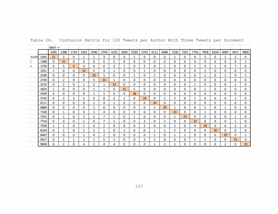
107
Table 28. Confusion Matrix for 120 Tweets per Author With Three Tweets per Document
label ‐>1045 1388 1734 1921 2546 2744 3155 3693 5599 5742 6111 6886 7100 7241 7754 7958 8164 8487 9417 9800
truth 1045 21 3 0 1 1 3 0 3 1 0 0 0 1 0 0 3 0 1 2 0| 1388 0 31 0 0 0 6 2 0 0 0 0 0 0 0 0 0 0 0 0 1v 1734 0 3 9 0 0 6 2 1 0 5 0 1 0 0 1 4 1 0 7 0
1921 1 0 0 32 0 4 1 0 0 1 0 0 0 0 0 1 0 0 0 02546 0 0 0 0 30 5 0 0 1 0 1 0 0 0 0 1 0 1 0 12744 0 2 0 0 3 34 1 0 0 0 0 0 0 0 0 0 0 0 0 03155 0 2 0 1 2 1 32 0 0 0 0 0 0 0 1 0 0 0 1 03693 1 0 0 0 1 1 0 31 5 0 0 0 0 0 0 1 0 0 0 05599 0 0 0 0 1 1 0 0 38 0 0 0 0 0 0 0 0 0 0 05742 0 2 2 2 0 8 2 1 0 18 0 1 2 0 1 0 0 0 1 06111 0 0 0 0 1 4 1 0 0 0 34 0 0 0 0 0 0 0 0 06886 0 0 0 0 1 6 0 0 0 0 1 29 1 0 0 1 0 1 0 07100 0 1 0 0 1 4 0 0 0 0 0 0 33 0 0 1 0 0 0 07241 0 1 0 3 2 7 1 0 1 0 0 0 1 23 0 0 0 0 1 07754 0 3 0 1 0 7 1 0 0 2 0 2 0 0 23 0 0 0 1 07958 1 1 0 1 0 2 0 0 0 2 0 0 2 0 0 29 0 0 2 08164 0 1 0 1 2 1 0 1 0 0 1 1 2 0 0 0 30 0 0 08487 0 0 0 1 4 2 0 0 0 0 1 0 1 1 0 0 0 29 0 19417 0 1 1 1 1 5 1 0 0 2 1 0 0 0 1 1 0 0 25 09800 0 2 0 4 1 4 4 0 0 0 1 2 1 0 0 0 0 2 0 19
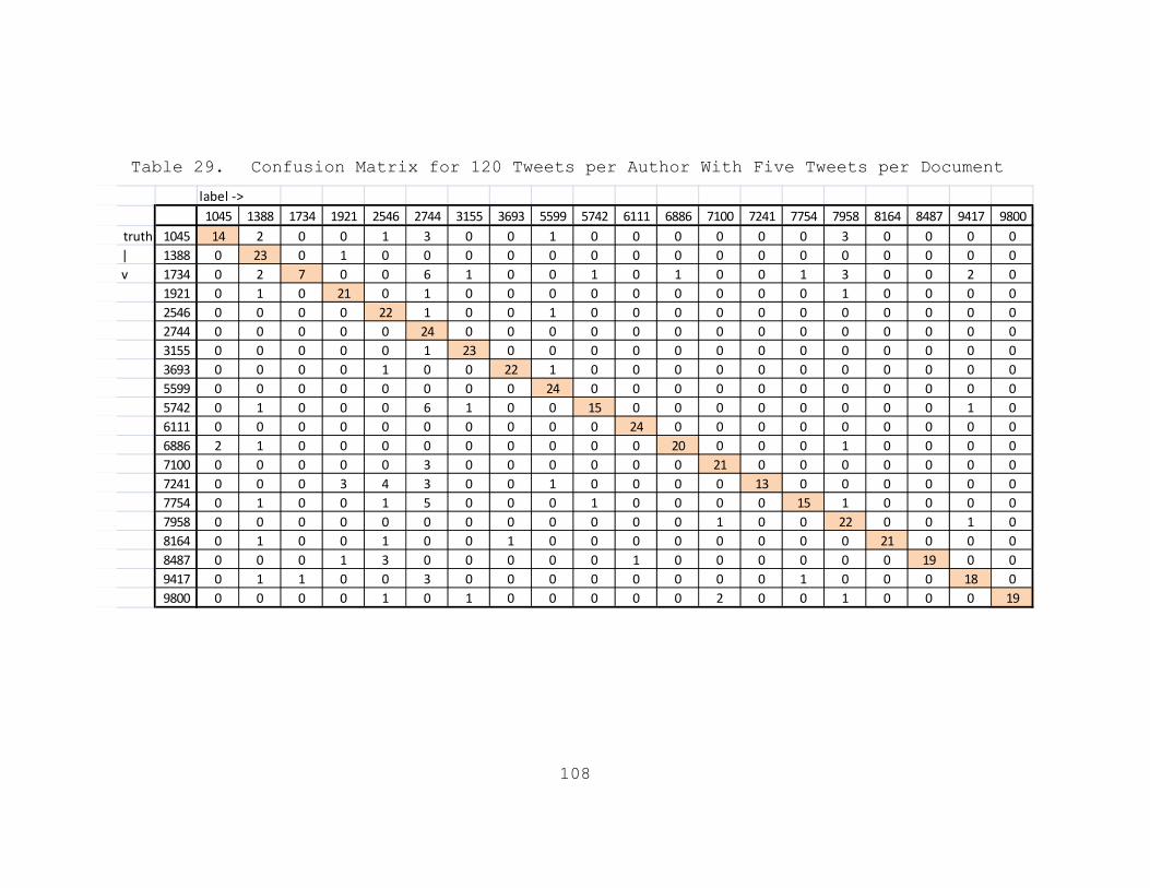
108
Table 29. Confusion Matrix for 120 Tweets per Author With Five Tweets per Document
label ‐>1045 1388 1734 1921 2546 2744 3155 3693 5599 5742 6111 6886 7100 7241 7754 7958 8164 8487 9417 9800
truth 1045 14 2 0 0 1 3 0 0 1 0 0 0 0 0 0 3 0 0 0 0| 1388 0 23 0 1 0 0 0 0 0 0 0 0 0 0 0 0 0 0 0 0v 1734 0 2 7 0 0 6 1 0 0 1 0 1 0 0 1 3 0 0 2 0
1921 0 1 0 21 0 1 0 0 0 0 0 0 0 0 0 1 0 0 0 02546 0 0 0 0 22 1 0 0 1 0 0 0 0 0 0 0 0 0 0 02744 0 0 0 0 0 24 0 0 0 0 0 0 0 0 0 0 0 0 0 03155 0 0 0 0 0 1 23 0 0 0 0 0 0 0 0 0 0 0 0 03693 0 0 0 0 1 0 0 22 1 0 0 0 0 0 0 0 0 0 0 05599 0 0 0 0 0 0 0 0 24 0 0 0 0 0 0 0 0 0 0 05742 0 1 0 0 0 6 1 0 0 15 0 0 0 0 0 0 0 0 1 06111 0 0 0 0 0 0 0 0 0 0 24 0 0 0 0 0 0 0 0 06886 2 1 0 0 0 0 0 0 0 0 0 20 0 0 0 1 0 0 0 07100 0 0 0 0 0 3 0 0 0 0 0 0 21 0 0 0 0 0 0 07241 0 0 0 3 4 3 0 0 1 0 0 0 0 13 0 0 0 0 0 07754 0 1 0 0 1 5 0 0 0 1 0 0 0 0 15 1 0 0 0 07958 0 0 0 0 0 0 0 0 0 0 0 0 1 0 0 22 0 0 1 08164 0 1 0 0 1 0 0 1 0 0 0 0 0 0 0 0 21 0 0 08487 0 0 0 1 3 0 0 0 0 0 1 0 0 0 0 0 0 19 0 09417 0 1 1 0 0 3 0 0 0 0 0 0 0 0 1 0 0 0 18 09800 0 0 0 0 1 0 1 0 0 0 0 0 2 0 0 1 0 0 0 19
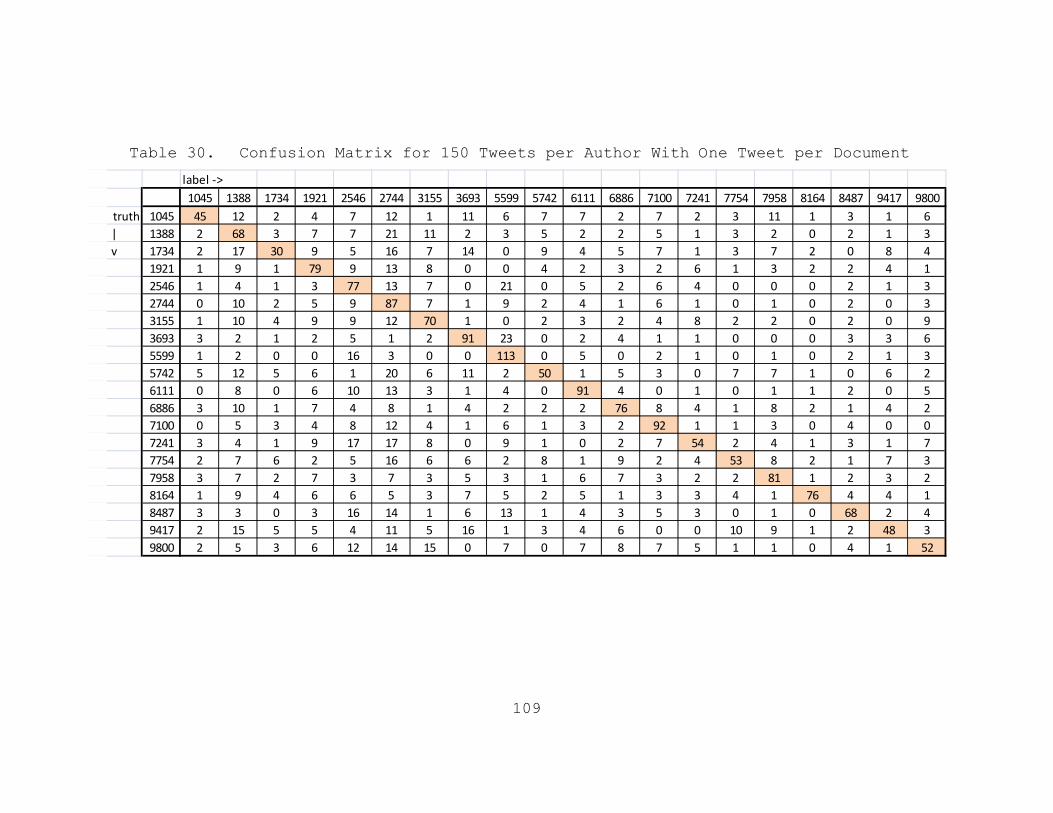
109
Table 30. Confusion Matrix for 150 Tweets per Author With One Tweet per Document
label ‐>1045 1388 1734 1921 2546 2744 3155 3693 5599 5742 6111 6886 7100 7241 7754 7958 8164 8487 9417 9800
truth 1045 45 12 2 4 7 12 1 11 6 7 7 2 7 2 3 11 1 3 1 6| 1388 2 68 3 7 7 21 11 2 3 5 2 2 5 1 3 2 0 2 1 3v 1734 2 17 30 9 5 16 7 14 0 9 4 5 7 1 3 7 2 0 8 4
1921 1 9 1 79 9 13 8 0 0 4 2 3 2 6 1 3 2 2 4 12546 1 4 1 3 77 13 7 0 21 0 5 2 6 4 0 0 0 2 1 32744 0 10 2 5 9 87 7 1 9 2 4 1 6 1 0 1 0 2 0 33155 1 10 4 9 9 12 70 1 0 2 3 2 4 8 2 2 0 2 0 93693 3 2 1 2 5 1 2 91 23 0 2 4 1 1 0 0 0 3 3 65599 1 2 0 0 16 3 0 0 113 0 5 0 2 1 0 1 0 2 1 35742 5 12 5 6 1 20 6 11 2 50 1 5 3 0 7 7 1 0 6 26111 0 8 0 6 10 13 3 1 4 0 91 4 0 1 0 1 1 2 0 56886 3 10 1 7 4 8 1 4 2 2 2 76 8 4 1 8 2 1 4 27100 0 5 3 4 8 12 4 1 6 1 3 2 92 1 1 3 0 4 0 07241 3 4 1 9 17 17 8 0 9 1 0 2 7 54 2 4 1 3 1 77754 2 7 6 2 5 16 6 6 2 8 1 9 2 4 53 8 2 1 7 37958 3 7 2 7 3 7 3 5 3 1 6 7 3 2 2 81 1 2 3 28164 1 9 4 6 6 5 3 7 5 2 5 1 3 3 4 1 76 4 4 18487 3 3 0 3 16 14 1 6 13 1 4 3 5 3 0 1 0 68 2 49417 2 15 5 5 4 11 5 16 1 3 4 6 0 0 10 9 1 2 48 39800 2 5 3 6 12 14 15 0 7 0 7 8 7 5 1 1 0 4 1 52

110
Table 31. Confusion Matrix for 150 Tweets per Author With Three Tweets per Document
label ‐>1045 1388 1734 1921 2546 2744 3155 3693 5599 5742 6111 6886 7100 7241 7754 7958 8164 8487 9417 9800
truth 1045 25 2 0 1 2 4 0 3 2 4 1 0 1 0 0 5 0 0 0 0| 1388 0 38 0 1 0 7 3 0 0 1 0 0 0 0 0 0 0 0 0 0v 1734 1 8 11 0 0 6 1 1 0 8 0 0 1 0 0 3 1 0 9 0
1921 0 3 0 41 1 3 0 0 0 1 0 0 0 0 0 1 0 0 0 02546 0 0 0 0 43 3 0 0 1 0 0 0 0 1 0 1 0 0 0 12744 0 1 0 0 2 46 0 0 0 0 0 0 0 0 0 0 0 1 0 03155 0 0 0 2 2 1 42 0 0 0 1 0 0 0 1 0 0 0 1 03693 0 0 0 0 3 0 0 40 5 0 0 0 0 0 0 0 0 0 1 15599 0 0 0 0 3 1 0 0 46 0 0 0 0 0 0 0 0 0 0 05742 1 3 2 2 0 8 2 2 1 24 0 0 0 0 2 2 0 0 1 06111 0 2 0 1 3 2 0 0 0 0 42 0 0 0 0 0 0 0 0 06886 0 2 0 0 0 3 0 0 0 0 0 41 2 1 0 0 0 0 1 07100 0 0 0 0 2 3 1 0 0 0 0 0 44 0 0 0 0 0 0 07241 0 2 0 6 5 2 2 0 1 0 0 1 1 29 0 0 1 0 0 07754 0 1 0 2 2 3 1 1 0 3 0 2 0 0 31 1 0 0 3 07958 3 0 0 0 0 2 0 0 0 0 0 0 2 0 0 42 0 0 1 08164 0 4 0 1 2 0 0 1 0 0 3 1 1 0 0 1 36 0 0 08487 1 0 0 0 6 1 1 0 0 0 2 0 1 0 0 0 0 36 1 19417 0 4 1 1 0 6 1 1 0 1 1 0 1 0 1 1 0 0 31 09800 0 2 0 1 2 2 3 0 0 0 0 2 2 0 0 0 0 0 0 36

111
Table 32. Confusion Matrix for 150 Tweets per Author With Five Tweets per Document
label ‐>1045 1388 1734 1921 2546 2744 3155 3693 5599 5742 6111 6886 7100 7241 7754 7958 8164 8487 9417 9800
truth 1045 20 2 0 0 0 2 0 0 0 1 0 0 2 0 0 3 0 0 0 0| 1388 0 26 0 0 0 2 2 0 0 0 0 0 0 0 0 0 0 0 0 0v 1734 0 5 8 0 0 5 1 0 0 3 0 1 0 0 0 1 0 0 6 0
1921 0 0 0 29 0 0 0 0 0 0 0 0 1 0 0 0 0 0 0 02546 0 0 0 0 29 0 0 0 0 0 0 1 0 0 0 0 0 0 0 02744 0 0 0 0 0 30 0 0 0 0 0 0 0 0 0 0 0 0 0 03155 0 0 0 0 1 0 28 0 0 0 0 0 0 1 0 0 0 0 0 03693 0 0 0 0 0 0 0 28 2 0 0 0 0 0 0 0 0 0 0 05599 0 0 0 0 0 0 0 0 30 0 0 0 0 0 0 0 0 0 0 05742 0 0 0 1 0 7 0 0 0 20 0 0 0 0 1 0 0 0 1 06111 0 0 0 0 1 0 0 0 0 0 29 0 0 0 0 0 0 0 0 06886 1 0 0 1 0 0 0 0 0 0 0 28 0 0 0 0 0 0 0 07100 0 0 0 0 0 3 0 0 0 0 0 0 27 0 0 0 0 0 0 07241 0 1 0 2 5 0 1 0 0 0 0 0 1 20 0 0 0 0 0 07754 0 1 1 0 0 5 0 0 0 1 0 0 0 0 19 1 0 0 2 07958 0 0 0 0 0 0 0 0 0 0 0 0 0 0 0 29 0 0 1 08164 0 1 0 0 1 0 0 0 0 1 0 0 0 0 0 1 26 0 0 08487 0 0 0 0 4 1 0 0 0 0 2 0 0 0 0 0 0 23 0 09417 0 2 0 0 0 3 0 0 0 0 0 1 0 0 1 0 0 0 23 09800 0 0 0 0 2 1 1 0 0 0 0 0 1 0 0 0 0 0 0 25

112
Table 33. Per Author Accuracy Rates for Various Total Tweets per Author and Tweets per Document
# TweetsTweets per Document 1 3 1 3 5 1 3 5 1 3 5
1045 0.133 0.5 0.12 0.294 0.5 0.283 0.525 0.583 0.3 0.5 0.6671388 0.2 0.6 0.42 0.824 0.9 0.4 0.775 0.958 0.453 0.76 0.8671734 0.033 0.1 0.08 0.059 0 0.183 0.225 0.292 0.2 0.22 0.2671921 0.133 0.2 0.3 0.294 0.3 0.508 0.8 0.875 0.527 0.82 0.9672546 0.367 0.7 0.3 0.647 0.9 0.483 0.75 0.917 0.513 0.86 0.9672744 0.333 0.6 0.4 0.588 0.9 0.617 0.85 1 0.58 0.92 13155 0.267 0.7 0.48 0.765 0.8 0.492 0.8 0.958 0.467 0.84 0.9333693 0.6 0.7 0.54 0.647 0.8 0.608 0.775 0.917 0.607 0.8 0.9335599 0.733 0.9 0.74 0.941 1 0.783 0.95 1 0.753 0.92 15742 0.067 0.1 0.14 0.294 0.2 0.325 0.45 0.625 0.333 0.48 0.6676111 0.467 0.6 0.5 0.471 0.8 0.542 0.85 1 0.607 0.84 0.9676886 0.3 0.4 0.26 0.294 0.4 0.492 0.725 0.833 0.507 0.82 0.9337100 0.267 0.5 0.36 0.529 0.7 0.533 0.825 0.875 0.613 0.88 0.97241 0.167 0.2 0.2 0.353 0.4 0.35 0.575 0.542 0.36 0.58 0.6677754 0.333 0.3 0.24 0.059 0.2 0.375 0.575 0.625 0.353 0.62 0.6337958 0.267 0.7 0.44 0.529 0.7 0.475 0.725 0.917 0.54 0.84 0.9678164 0.467 0.7 0.36 0.471 0.7 0.442 0.75 0.875 0.507 0.72 0.8678487 0.267 0.4 0.38 0.588 0.7 0.442 0.725 0.792 0.453 0.72 0.7679417 0.333 0.6 0.26 0.412 0.5 0.342 0.625 0.75 0.32 0.62 0.7679800 0.167 0.3 0.18 0.235 0.4 0.317 0.475 0.792 0.347 0.72 0.833
30 50 120 150

113
APPENDIX C: TWEET SEND TIME ADDITIONAL DATA
Figure 31. Author 1045 Tweet Send Time Histogram
Figure 32. Author 1388 Tweet Send Time Histogram

114
Figure 33. Author 1734 Tweet Send Time Histogram
Figure 34. Author 1921 Tweet Send Time Histogram

115
Figure 35. Author 2546 Tweet Send Time Histogram
Figure 36. Author 2744 Tweet Send Time Histogram
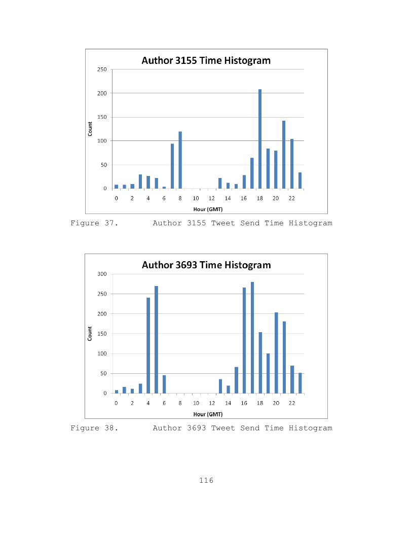
116
Figure 37. Author 3155 Tweet Send Time Histogram
Figure 38. Author 3693 Tweet Send Time Histogram
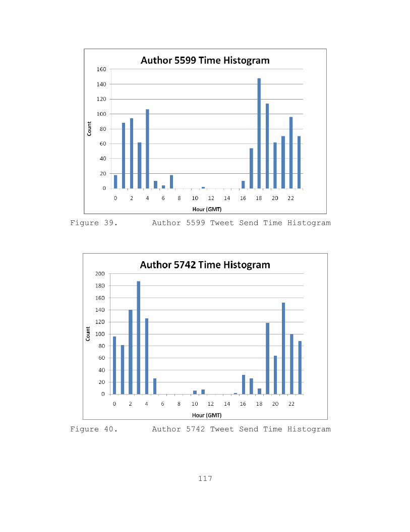
117
Figure 39. Author 5599 Tweet Send Time Histogram
Figure 40. Author 5742 Tweet Send Time Histogram

118
Figure 41. Author 6111 Tweet Send Time Histogram
Figure 42. Author 6886 Tweet Send Time Histogram

119
Figure 43. Author 7100 Tweet Send Time Histogram
Figure 44. Author 7241 Tweet Send Time Histogram

120
Figure 45. Author 7754 Tweet Send Time Histogram
Figure 46. Author 7958 Tweet Send Time Histogram

121
Figure 47. Author 8164 Tweet Send Time Histogram
Figure 48. Author 8487 Tweet Send Time Histogram

122
Figure 49. Author 9417 Tweet Send Time Histogram
Figure 50. Author 9800 Tweet Send Time Histogram

123
APPENDIX D: PHONE CLASSIFIER ADDITIONAL DATA
Table 34. Confusion Matrix for 30 Signal Vectors per Phone With One Signal Vector per Training Set
labeltruth bberry htc371 htc373 htc374 htc375 htc376 htc601 htc_rob iphone4 iphone5 iphone7 n8_594 n97_430 n97_444 n97_618 n97_620 nok_128 nok_e5 nok_e62 treo
bberry 29 0 0 0 0 0 0 0 0 0 0 0 0 0 0 1 0 0 0 0htc371 0 27 2 0 0 0 0 0 0 0 0 0 0 0 0 0 1 0 0 0htc373 0 1 28 0 0 0 0 0 0 0 0 0 0 0 0 0 0 0 2 0htc374 0 0 0 25 0 4 0 0 0 0 0 0 0 0 0 0 0 0 1 0htc375 0 0 0 0 28 0 0 1 0 0 0 0 0 0 0 0 0 0 0 1htc376 1 0 1 5 0 22 0 0 0 0 0 0 0 0 0 0 0 0 1 0htc601 0 0 0 0 0 0 30 0 0 0 0 0 0 0 0 0 0 0 0 0htc_rob 0 0 0 0 0 0 0 28 0 0 1 0 0 0 0 0 0 0 1 0iphone4 1 0 0 0 0 0 0 0 22 3 1 3 0 0 0 0 0 0 0 0iphone5 0 0 0 0 0 0 0 0 6 21 3 0 0 0 0 0 0 0 0 0iphone7 1 0 0 0 0 0 1 2 3 6 9 0 0 3 2 0 1 2 0 0n8_594 0 0 0 0 0 0 0 0 0 0 0 30 0 0 0 0 0 0 0 0n97_430 0 0 0 0 0 0 0 0 0 0 0 2 27 0 0 1 0 0 0 0n97_444 0 0 0 0 0 0 0 0 0 0 0 2 1 24 0 1 2 0 0 0n97_618 0 0 0 0 0 0 0 0 0 0 1 0 0 0 26 0 0 0 3 0n97_620 0 0 0 0 0 0 0 0 0 0 0 1 6 2 0 21 0 0 0 0nok_128 4 2 0 0 0 0 0 0 0 0 0 1 1 5 4 1 11 1 0 0nok_e5 0 0 0 0 0 0 0 0 0 0 0 0 0 0 3 0 0 27 0 0nok_e62 0 0 1 1 0 0 0 2 0 0 0 0 0 0 0 0 0 0 26 0treo 0 0 0 0 1 0 0 0 0 0 0 0 0 0 0 0 0 0 0 29

124
Table 35. Confusion Matrix for 30 Signal Vectors per Phone With Two Signal Vectors per Training Set
labelbberry htc371 htc373 htc374 htc375 htc376 htc601 htc_rob iphone4 iphone5 iphone7 n8_594 n97_430 n97_444 n97_618 n97_620 nok_128 nok_e5 nok_e62 treo
truth bberry 15 0 0 0 0 0 0 0 0 0 0 0 0 0 0 0 0 0 0 0htc371 0 11 3 0 0 0 0 0 0 0 0 0 0 1 0 0 0 0 0 0htc373 0 2 13 0 0 0 0 0 0 0 0 0 0 0 0 0 0 0 0 0htc374 0 0 0 11 0 4 0 0 0 0 0 0 0 0 0 0 0 0 0 0htc375 0 0 0 0 14 0 0 0 1 0 0 0 0 0 0 0 0 0 0 0htc376 0 0 0 3 0 12 0 0 0 0 0 0 0 0 0 0 0 0 0 0htc601 0 0 0 0 0 0 15 0 0 0 0 0 0 0 0 0 0 0 0 0htc_rob 0 0 0 0 0 0 0 14 0 0 0 0 0 0 0 0 0 0 1 0iphone4 0 0 0 0 0 0 0 0 11 2 2 0 0 0 0 0 0 0 0 0iphone5 0 0 0 0 0 0 0 0 1 11 2 0 0 0 0 0 1 0 0 0iphone7 0 0 0 0 0 0 0 2 2 6 4 0 0 1 0 0 0 0 0 0n8_594 0 0 0 0 0 0 0 0 0 0 0 15 0 0 0 0 0 0 0 0n97_430 0 0 0 0 0 0 0 0 0 0 0 0 15 0 0 0 0 0 0 0n97_444 0 0 0 0 0 0 0 0 0 0 0 0 0 15 0 0 0 0 0 0n97_618 0 0 0 0 0 0 0 0 0 0 0 0 0 0 14 0 0 1 0 0n97_620 0 0 0 0 0 0 0 0 0 0 0 1 2 0 0 12 0 0 0 0nok_128 0 1 0 0 0 0 0 0 0 0 0 1 0 3 4 1 4 1 0 0nok_e5 0 0 0 0 0 0 1 0 0 0 0 0 0 0 2 0 0 12 0 0nok_e62 0 0 0 0 0 0 0 0 0 0 0 0 0 0 0 0 0 0 15 0treo 0 0 0 0 0 0 0 0 0 0 0 0 0 0 0 0 0 0 0 15

125
Table 36. Confusion Matrix for 30 Signal Vectors per Phone With Three Signal Vectors per Training Set
labelbberry htc371 htc373 htc374 htc375 htc376 htc601 htc_rob iphone4 iphone5 iphone7 n8_594 n97_430 n97_444 n97_618 n97_620 nok_128 nok_e5 nok_e62 treo
truth bberry 10 0 0 0 0 0 0 0 0 0 0 0 0 0 0 0 0 0 0 0htc371 0 10 0 0 0 0 0 0 0 0 0 0 0 0 0 0 0 0 0 0htc373 0 2 8 0 0 0 0 0 0 0 0 0 0 0 0 0 0 0 0 0htc374 0 0 0 7 0 3 0 0 0 0 0 0 0 0 0 0 0 0 0 0htc375 0 0 0 0 10 0 0 0 0 0 0 0 0 0 0 0 0 0 0 0htc376 0 0 0 1 0 9 0 0 0 0 0 0 0 0 0 0 0 0 0 0htc601 0 0 0 0 0 0 10 0 0 0 0 0 0 0 0 0 0 0 0 0htc_rob 0 0 0 0 0 0 0 10 0 0 0 0 0 0 0 0 0 0 0 0iphone4 0 0 0 0 0 0 0 0 7 1 1 1 0 0 0 0 0 0 0 0iphone5 0 0 0 0 0 0 0 0 1 7 2 0 0 0 0 0 0 0 0 0iphone7 0 0 0 0 0 0 0 1 0 5 2 0 0 1 0 0 0 1 0 0n8_594 0 0 0 0 0 0 0 0 0 0 0 10 0 0 0 0 0 0 0 0n97_430 0 0 0 0 0 0 0 0 0 0 0 0 10 0 0 0 0 0 0 0n97_444 0 0 0 0 0 0 0 0 0 0 0 0 0 8 0 1 1 0 0 0n97_618 0 0 0 0 0 0 0 0 0 0 0 0 1 0 9 0 0 0 0 0n97_620 0 0 0 0 0 0 0 0 0 0 0 2 1 0 0 7 0 0 0 0nok_128 1 0 0 0 0 0 0 0 0 0 1 0 0 2 1 1 4 0 0 0nok_e5 0 0 0 0 0 0 0 0 0 0 0 0 0 0 2 0 0 8 0 0nok_e62 0 0 0 0 0 0 0 0 0 0 0 0 0 0 0 0 0 0 10 0treo 0 0 0 0 0 0 0 0 0 0 0 0 0 0 0 0 0 0 0 10

126
Table 37. Confusion Matrix for 50 Signal Vectors per Phone With One Signal Vector per Training Set
labelbberry htc_rob htc371 htc373 htc374 htc375 htc376 htc601 iphone4 iphone5 iphone7 n8_594 n97_430 n97_444 n97_618 n97_620 nok_128 nok_e5 nok_e62 treo
truth bberry 49 0 1 0 0 0 0 0 0 0 0 0 0 0 0 0 0 0 0 0htc_rob 0 47 0 0 0 1 0 0 0 0 1 0 0 0 0 0 0 0 1 0htc371 0 0 46 3 0 0 0 0 0 0 0 0 0 1 0 0 0 0 0 0htc373 0 0 0 49 1 0 0 0 0 0 0 0 0 0 0 0 0 0 0 0htc374 0 0 0 0 43 0 6 0 0 0 0 0 0 0 0 0 0 0 1 0htc375 0 1 0 0 0 49 0 0 0 0 0 0 0 0 0 0 0 0 0 0htc376 1 0 1 1 14 0 30 0 0 0 0 0 0 0 0 0 0 0 2 1htc601 0 0 0 0 0 0 0 50 0 0 0 0 0 0 0 0 0 0 0 0iphone4 0 0 0 0 0 0 0 2 43 4 0 1 0 0 0 0 0 0 0 0iphone5 0 0 0 0 0 0 0 0 8 36 6 0 0 0 0 0 0 0 0 0iphone7 1 1 0 0 0 1 0 0 4 13 23 0 0 2 1 0 2 2 0 0n8_594 0 0 0 0 0 0 0 0 0 0 0 47 0 0 0 1 2 0 0 0n97_430 0 0 0 0 0 0 0 0 0 0 0 1 47 0 0 2 0 0 0 0n97_444 0 0 0 0 0 0 0 0 0 0 0 1 1 45 0 1 2 0 0 0n97_618 0 0 0 0 0 0 0 0 0 0 0 0 1 0 43 0 1 5 0 0n97_620 0 0 0 0 0 0 0 0 0 0 0 1 7 1 0 41 0 0 0 0nok_128 5 0 1 0 0 0 0 0 0 0 4 1 2 11 5 3 16 2 0 0nok_e5 0 0 0 0 0 0 0 3 0 0 0 0 0 0 2 0 0 45 0 0nok_e62 0 0 0 0 2 1 1 0 0 0 0 0 0 0 0 0 0 0 46 0treo 0 0 0 0 0 0 0 0 0 0 0 0 0 0 0 0 0 0 0 50

127
Table 38. Confusion Matrix for 50 Signal Vectors per Phone With Two Signal Vectors per Training Set
labelbberry htc_rob htc371 htc373 htc374 htc375 htc376 htc601 iphone4 iphone5 iphone7 n8_594 n97_430 n97_444 n97_618 n97_620 nok_128 nok_e5 nok_e62 treo
truth bberry 24 0 0 0 0 0 0 0 0 0 0 0 0 0 1 0 0 0 0 0htc_rob 0 25 0 0 0 0 0 0 0 0 0 0 0 0 0 0 0 0 0 0htc371 0 0 25 0 0 0 0 0 0 0 0 0 0 0 0 0 0 0 0 0htc373 0 0 1 24 0 0 0 0 0 0 0 0 0 0 0 0 0 0 0 0htc374 0 0 0 0 23 0 2 0 0 0 0 0 0 0 0 0 0 0 0 0htc375 0 0 0 0 0 24 0 0 1 0 0 0 0 0 0 0 0 0 0 0htc376 0 0 0 0 4 0 21 0 0 0 0 0 0 0 0 0 0 0 0 0htc601 0 0 0 0 0 0 0 25 0 0 0 0 0 0 0 0 0 0 0 0iphone4 0 0 0 0 0 0 0 0 22 3 0 0 0 0 0 0 0 0 0 0iphone5 0 0 0 0 0 0 0 0 2 20 3 0 0 0 0 0 0 0 0 0iphone7 0 1 0 0 0 0 0 0 1 9 9 0 0 1 0 0 3 1 0 0n8_594 0 0 0 0 0 0 0 0 0 0 0 24 1 0 0 0 0 0 0 0n97_430 0 0 0 0 0 0 0 0 0 0 0 0 25 0 0 0 0 0 0 0n97_444 0 0 0 0 0 0 0 0 0 0 0 0 0 25 0 0 0 0 0 0n97_618 0 0 0 0 0 0 0 0 0 0 0 0 0 0 24 0 0 1 0 0n97_620 0 0 0 0 0 0 0 0 0 0 0 0 2 0 0 23 0 0 0 0nok_128 1 0 0 0 0 0 0 0 0 0 1 0 0 2 4 1 14 2 0 0nok_e5 0 0 0 0 0 0 0 0 0 0 0 0 0 0 2 0 0 23 0 0nok_e62 0 0 0 0 1 0 0 0 0 0 0 0 0 0 0 0 0 0 24 0treo 0 0 0 0 0 0 0 0 0 0 0 0 0 0 0 0 0 0 0 25

128
Table 39. Confusion Matrix for 50 Signal Vectors per Phone With Three Signal Vectors per Training Set
labelbberry htc_rob htc371 htc373 htc374 htc375 htc376 htc601 iphone4 iphone5 iphone7 n8_594 n97_430 n97_444 n97_618 n97_620 nok_128 nok_e5 nok_e62 treo
truth bberry 16 0 0 0 0 0 0 0 0 0 0 0 0 0 0 0 1 0 0 0htc_rob 0 16 0 0 0 0 0 0 0 0 0 0 0 0 0 0 0 0 1 0htc371 0 0 17 0 0 0 0 0 0 0 0 0 0 0 0 0 0 0 0 0htc373 0 0 0 17 0 0 0 0 0 0 0 0 0 0 0 0 0 0 0 0htc374 0 0 0 0 16 0 1 0 0 0 0 0 0 0 0 0 0 0 0 0htc375 0 0 0 0 0 17 0 0 0 0 0 0 0 0 0 0 0 0 0 0htc376 0 0 0 0 4 0 12 0 0 0 0 0 0 0 0 0 0 0 1 0htc601 0 0 0 0 0 0 0 17 0 0 0 0 0 0 0 0 0 0 0 0iphone4 0 0 0 0 0 0 0 0 15 1 1 0 0 0 0 0 0 0 0 0iphone5 0 0 0 0 0 0 0 0 1 15 1 0 0 0 0 0 0 0 0 0iphone7 0 0 0 0 0 0 0 0 0 7 9 0 0 1 0 0 0 0 0 0n8_594 0 0 0 0 0 0 0 0 0 0 0 17 0 0 0 0 0 0 0 0n97_430 0 0 0 0 0 0 0 0 0 0 0 0 17 0 0 0 0 0 0 0n97_444 0 0 0 0 0 0 0 0 0 0 0 0 0 17 0 0 0 0 0 0n97_618 0 0 0 0 0 0 0 0 0 0 0 0 0 0 17 0 0 0 0 0n97_620 0 0 0 0 0 0 0 0 0 0 0 0 2 0 0 15 0 0 0 0nok_128 1 0 0 0 0 0 0 0 0 1 2 0 0 1 1 0 10 1 0 0nok_e5 0 0 0 0 0 0 0 0 0 0 0 0 0 0 0 0 0 17 0 0nok_e62 0 0 0 0 1 0 0 0 0 0 0 0 0 0 0 0 0 0 16 0treo 0 0 0 0 0 0 0 0 0 0 0 0 0 0 0 0 0 0 0 17

129
Table 40. Confusion Matrix for 50 Signal Vectors per Phone With Four Signal Vectors per Training Set
labelbberry htc_rob htc371 htc373 htc374 htc375 htc376 htc601 iphone4 iphone5 iphone7 n8_594 n97_430 n97_444 n97_618 n97_620 nok_128 nok_e5 nok_e62 treo
truth bberry 13 0 0 0 0 0 0 0 0 0 0 0 0 0 0 0 0 0 0 0htc_rob 0 13 0 0 0 0 0 0 0 0 0 0 0 0 0 0 0 0 0 0htc371 0 0 13 0 0 0 0 0 0 0 0 0 0 0 0 0 0 0 0 0htc373 0 0 0 13 0 0 0 0 0 0 0 0 0 0 0 0 0 0 0 0htc374 0 0 0 0 13 0 0 0 0 0 0 0 0 0 0 0 0 0 0 0htc375 0 0 0 0 0 13 0 0 0 0 0 0 0 0 0 0 0 0 0 0htc376 0 0 0 0 2 0 11 0 0 0 0 0 0 0 0 0 0 0 0 0htc601 0 0 0 0 0 0 0 13 0 0 0 0 0 0 0 0 0 0 0 0iphone4 0 0 0 0 0 0 0 0 11 1 1 0 0 0 0 0 0 0 0 0iphone5 0 0 0 0 0 0 0 0 1 10 2 0 0 0 0 0 0 0 0 0iphone7 0 0 0 0 0 0 0 0 0 5 7 0 0 1 0 0 0 0 0 0n8_594 0 0 0 0 0 0 0 0 0 0 0 13 0 0 0 0 0 0 0 0n97_430 0 0 0 0 0 0 0 0 0 0 0 0 13 0 0 0 0 0 0 0n97_444 0 0 0 0 0 0 0 0 0 0 0 0 0 13 0 0 0 0 0 0n97_618 0 0 0 0 0 0 0 0 0 0 0 0 0 0 13 0 0 0 0 0n97_620 0 0 0 0 0 0 0 0 0 0 0 0 0 0 0 13 0 0 0 0nok_128 0 0 0 0 0 0 0 0 0 0 1 0 0 1 1 0 10 0 0 0nok_e5 0 0 0 0 0 0 0 0 0 0 0 0 0 0 0 0 0 13 0 0nok_e62 0 0 0 0 1 0 0 0 0 0 0 0 0 0 0 0 0 0 12 0treo 0 0 0 0 0 0 0 0 0 0 0 0 0 0 0 0 0 0 0 13

130
Table 41. Confusion Matrix for 50 Signal Vectors per Phone With Five Signal Vectors per Training Set
labelbberry htc_rob htc371 htc373 htc374 htc375 htc376 htc601 iphone4 iphone5 iphone7 n8_594 n97_430 n97_444 n97_618 n97_620 nok_128 nok_e5 nok_e62 treo
truth bberry 10 0 0 0 0 0 0 0 0 0 0 0 0 0 0 0 0 0 0 0htc_rob 0 10 0 0 0 0 0 0 0 0 0 0 0 0 0 0 0 0 0 0htc371 0 0 10 0 0 0 0 0 0 0 0 0 0 0 0 0 0 0 0 0htc373 0 0 0 10 0 0 0 0 0 0 0 0 0 0 0 0 0 0 0 0htc374 0 0 0 0 8 0 2 0 0 0 0 0 0 0 0 0 0 0 0 0htc375 0 0 0 0 0 10 0 0 0 0 0 0 0 0 0 0 0 0 0 0htc376 0 0 0 0 1 0 9 0 0 0 0 0 0 0 0 0 0 0 0 0htc601 0 0 0 0 0 0 0 10 0 0 0 0 0 0 0 0 0 0 0 0iphone4 0 0 0 0 0 0 0 0 10 0 0 0 0 0 0 0 0 0 0 0iphone5 0 0 0 0 0 0 0 0 1 8 1 0 0 0 0 0 0 0 0 0iphone7 0 0 0 0 0 0 0 0 0 3 6 0 0 0 0 0 1 0 0 0n8_594 0 0 0 0 0 0 0 0 0 0 0 10 0 0 0 0 0 0 0 0n97_430 0 0 0 0 0 0 0 0 0 0 0 0 10 0 0 0 0 0 0 0n97_444 0 0 0 0 0 0 0 0 0 0 0 0 0 9 0 0 1 0 0 0n97_618 0 0 0 0 0 0 0 0 0 0 0 0 0 0 10 0 0 0 0 0n97_620 0 0 0 0 0 0 0 0 0 0 0 0 0 0 0 10 0 0 0 0nok_128 1 0 0 0 0 0 0 0 0 0 1 0 0 1 0 0 7 0 0 0nok_e5 0 0 0 0 0 0 0 0 0 0 0 0 0 0 0 0 0 10 0 0nok_e62 0 0 0 0 0 0 0 0 0 0 0 0 0 0 0 0 0 0 10 0treo 0 0 0 0 0 0 0 0 0 0 0 0 0 0 0 0 0 0 0 10

131
Table 42. Confusion Matrix for 100 Signal Vectors per Phone With One Signal Vector per Training Set
labelbberry htc_rob htc371 htc373 htc374 htc375 htc376 htc601 iphone4 iphone5 iphone7 n8_594 n97_430 n97_444 n97_618 n97_620 nok_128 nok_e5 nok_e62 treo
truth bberry 96 0 1 0 0 0 0 0 0 0 0 0 0 0 0 0 3 0 0 0htc_rob 0 100 0 0 0 0 0 0 0 0 0 0 0 0 0 0 0 0 0 0htc371 1 0 94 5 0 0 0 0 0 0 0 0 0 0 0 0 0 0 0 0htc373 0 0 1 99 0 0 0 0 0 0 0 0 0 0 0 0 0 0 0 0htc374 0 0 0 0 89 0 10 0 0 0 0 0 0 0 0 0 0 0 1 0htc375 0 1 0 0 0 99 0 0 0 0 0 0 0 0 0 0 0 0 0 0htc376 1 1 0 0 29 0 67 0 0 0 0 0 0 0 0 0 0 0 2 0htc601 0 0 0 0 1 0 0 97 0 0 0 0 0 0 0 0 0 2 0 0iphone4 0 0 0 0 0 0 0 1 84 12 0 0 0 0 0 0 3 0 0 0iphone5 0 0 0 0 0 0 0 0 7 83 10 0 0 0 0 0 0 0 0 0iphone7 1 0 0 0 0 1 0 2 8 20 59 0 0 2 0 0 4 3 0 0n8_594 0 0 0 0 0 0 0 1 0 0 0 98 1 0 0 0 0 0 0 0n97_430 0 0 0 0 0 0 0 0 0 0 0 0 98 0 0 2 0 0 0 0n97_444 0 0 0 0 0 0 0 0 0 0 0 0 1 91 0 0 8 0 0 0n97_618 0 0 1 0 0 0 0 0 0 0 0 0 1 0 89 0 1 8 0 0n97_620 0 0 0 0 0 0 0 0 0 0 0 0 4 1 0 95 0 0 0 0nok_128 13 0 1 0 0 0 0 0 0 0 4 0 2 20 4 1 51 4 0 0nok_e5 0 0 0 0 0 0 0 4 0 0 0 0 0 0 3 0 0 93 0 0nok_e62 0 0 0 0 2 2 0 0 0 0 0 0 0 0 0 0 0 0 96 0treo 0 0 0 0 0 0 0 0 0 0 0 0 0 0 0 0 0 0 0 100

132
Table 43. Confusion Matrix for 100 Signal Vectors per Phone With Two Signal Vectors per Training Set
labelbberry htc_rob htc371 htc373 htc374 htc375 htc376 htc601 iphone4 iphone5 iphone7 n8_594 n97_430 n97_444 n97_618 n97_620 nok_128 nok_e5 nok_e62 treo
truth bberry 49 0 1 0 0 0 0 0 0 0 0 0 0 0 0 0 0 0 0 0htc_rob 0 50 0 0 0 0 0 0 0 0 0 0 0 0 0 0 0 0 0 0htc371 0 0 50 0 0 0 0 0 0 0 0 0 0 0 0 0 0 0 0 0htc373 0 0 0 50 0 0 0 0 0 0 0 0 0 0 0 0 0 0 0 0htc374 0 0 0 0 49 0 1 0 0 0 0 0 0 0 0 0 0 0 0 0htc375 0 0 0 0 0 50 0 0 0 0 0 0 0 0 0 0 0 0 0 0htc376 0 0 0 0 5 0 44 0 0 0 0 0 0 0 0 0 0 0 1 0htc601 0 0 0 0 0 0 0 50 0 0 0 0 0 0 0 0 0 0 0 0iphone4 0 0 0 0 0 0 0 0 49 1 0 0 0 0 0 0 0 0 0 0iphone5 0 0 0 0 0 0 0 0 3 44 3 0 0 0 0 0 0 0 0 0iphone7 1 0 0 0 0 0 0 0 1 6 41 0 0 1 0 0 0 0 0 0n8_594 0 0 0 0 0 0 0 0 0 0 0 50 0 0 0 0 0 0 0 0n97_430 0 0 0 0 0 0 0 0 0 0 0 0 50 0 0 0 0 0 0 0n97_444 0 0 0 0 0 0 0 0 0 0 0 0 0 50 0 0 0 0 0 0n97_618 0 0 0 0 0 0 0 0 0 0 0 0 0 0 50 0 0 0 0 0n97_620 0 0 0 0 0 0 0 0 0 0 0 0 0 0 0 50 0 0 0 0nok_128 4 0 0 0 0 0 0 0 0 0 1 0 0 4 1 0 40 0 0 0nok_e5 0 0 0 0 0 0 0 0 0 0 0 0 0 0 0 0 0 50 0 0nok_e62 0 0 0 0 0 0 0 0 0 0 0 0 0 0 0 0 0 0 50 0treo 0 0 0 0 0 0 0 0 0 0 0 0 0 0 0 0 0 0 0 50

133
Table 44. Confusion Matrix for 100 Signal Vectors per Phone With Three Signal Vectors per Training Set
labelbberry htc_rob htc371 htc373 htc374 htc375 htc376 htc601 iphone4 iphone5 iphone7 n8_594 n97_430 n97_444 n97_618 n97_620 nok_128 nok_e5 nok_e62 treo
truth bberry 34 0 0 0 0 0 0 0 0 0 0 0 0 0 0 0 0 0 0 0htc_rob 0 34 0 0 0 0 0 0 0 0 0 0 0 0 0 0 0 0 0 0htc371 0 0 34 0 0 0 0 0 0 0 0 0 0 0 0 0 0 0 0 0htc373 0 0 0 34 0 0 0 0 0 0 0 0 0 0 0 0 0 0 0 0htc374 0 0 0 0 34 0 0 0 0 0 0 0 0 0 0 0 0 0 0 0htc375 0 0 0 0 0 34 0 0 0 0 0 0 0 0 0 0 0 0 0 0htc376 0 0 0 0 3 0 31 0 0 0 0 0 0 0 0 0 0 0 0 0htc601 0 0 0 0 0 0 0 34 0 0 0 0 0 0 0 0 0 0 0 0iphone4 0 0 0 0 0 0 0 0 33 1 0 0 0 0 0 0 0 0 0 0iphone5 0 0 0 0 0 0 0 0 0 33 1 0 0 0 0 0 0 0 0 0iphone7 0 0 0 0 0 0 0 0 0 4 30 0 0 0 0 0 0 0 0 0n8_594 0 0 0 0 0 0 0 0 0 0 0 34 0 0 0 0 0 0 0 0n97_430 0 0 0 0 0 0 0 0 0 0 0 0 34 0 0 0 0 0 0 0n97_444 0 0 0 0 0 0 0 0 0 0 0 0 0 34 0 0 0 0 0 0n97_618 0 0 0 0 0 0 0 0 0 0 0 0 0 0 34 0 0 0 0 0n97_620 0 0 0 0 0 0 0 0 0 0 0 0 0 0 0 34 0 0 0 0nok_128 4 0 0 0 0 0 0 0 0 0 0 0 0 1 0 0 29 0 0 0nok_e5 0 0 0 0 0 0 0 0 0 0 0 0 0 0 0 0 0 34 0 0nok_e62 0 0 0 0 0 0 0 0 0 0 0 0 0 0 0 0 0 0 34 0treo 0 0 0 0 0 0 0 0 0 0 0 0 0 0 0 0 0 0 0 34

134
Table 45. Confusion Matrix for 120 Signal Vectors per Phone With One Signal Vector per Training Set
labelbberry htc_rob htc371 htc373 htc374 htc375 htc376 htc601 iphone4 iphone5 iphone7 n8_594 n97_430 n97_444 n97_618 n97_620 nok_128 nok_e5 nok_e62 treo
truth bberry 117 0 0 0 0 0 0 0 0 0 0 0 0 0 0 0 3 0 0 0htc_rob 0 120 0 0 0 0 0 0 0 0 0 0 0 0 0 0 0 0 0 0htc371 1 0 113 5 0 0 0 0 0 0 0 0 0 0 0 0 0 1 0 0htc373 0 0 0 120 0 0 0 0 0 0 0 0 0 0 0 0 0 0 0 0htc374 0 0 0 0 111 0 8 0 0 0 0 0 0 0 0 0 0 0 1 0htc375 0 1 0 0 0 119 0 0 0 0 0 0 0 0 0 0 0 0 0 0htc376 1 0 0 0 35 1 81 0 0 0 0 0 0 0 0 0 0 0 2 0htc601 0 0 0 0 1 0 0 119 0 0 0 0 0 0 0 0 0 0 0 0iphone4 0 0 0 0 0 0 0 1 110 8 1 0 0 0 0 0 0 0 0 0iphone5 0 0 0 0 0 0 0 0 11 96 13 0 0 0 0 0 0 0 0 0iphone7 1 2 0 0 0 0 0 2 6 25 70 0 0 4 2 0 6 2 0 0n8_594 0 0 0 0 0 0 0 0 0 0 0 119 1 0 0 0 0 0 0 0n97_430 0 0 0 0 0 0 0 0 0 0 0 0 113 0 0 7 0 0 0 0n97_444 0 0 0 0 0 0 0 0 0 0 0 1 1 112 0 0 6 0 0 0n97_618 0 0 0 0 0 0 0 0 0 0 1 0 0 0 109 0 1 9 0 0n97_620 0 0 0 0 0 0 0 0 0 0 0 0 7 1 0 112 0 0 0 0nok_128 17 0 0 0 0 0 0 0 0 0 4 0 1 18 9 1 66 4 0 0nok_e5 0 0 0 0 0 0 1 2 0 0 0 0 0 0 2 0 0 115 0 0nok_e62 0 0 0 0 1 1 0 0 0 0 0 0 0 0 0 0 0 0 118 0treo 0 0 0 0 0 0 0 0 0 0 0 0 0 0 0 0 0 0 0 120

135
Table 46. Confusion Matrix for 120 Signal Vectors per Phone With Two Signal Vectors per Training Set
labelbberry htc_rob htc371 htc373 htc374 htc375 htc376 htc601 iphone4 iphone5 iphone7 n8_594 n97_430 n97_444 n97_618 n97_620 nok_128 nok_e5 nok_e62 treo
truth bberry 60 0 0 0 0 0 0 0 0 0 0 0 0 0 0 0 0 0 0 0htc_rob 0 60 0 0 0 0 0 0 0 0 0 0 0 0 0 0 0 0 0 0htc371 0 0 60 0 0 0 0 0 0 0 0 0 0 0 0 0 0 0 0 0htc373 0 0 0 60 0 0 0 0 0 0 0 0 0 0 0 0 0 0 0 0htc374 0 0 0 0 59 0 1 0 0 0 0 0 0 0 0 0 0 0 0 0htc375 0 0 0 0 0 60 0 0 0 0 0 0 0 0 0 0 0 0 0 0htc376 0 0 0 0 8 0 52 0 0 0 0 0 0 0 0 0 0 0 0 0htc601 0 0 0 0 0 0 0 60 0 0 0 0 0 0 0 0 0 0 0 0iphone4 0 0 0 0 0 0 0 0 58 2 0 0 0 0 0 0 0 0 0 0iphone5 0 0 0 0 0 0 0 0 2 53 5 0 0 0 0 0 0 0 0 0iphone7 0 0 0 0 0 0 0 0 2 12 45 0 0 0 0 0 1 0 0 0n8_594 0 0 0 0 0 0 0 0 0 0 0 60 0 0 0 0 0 0 0 0n97_430 0 0 0 0 0 0 0 0 0 0 0 0 60 0 0 0 0 0 0 0n97_444 0 0 0 0 0 0 0 0 0 0 0 0 0 60 0 0 0 0 0 0n97_618 0 0 0 0 0 0 0 0 0 0 0 0 0 0 60 0 0 0 0 0n97_620 0 0 0 0 0 0 0 0 0 0 0 0 0 0 0 60 0 0 0 0nok_128 4 0 0 0 0 0 0 0 0 0 1 0 0 8 1 0 45 1 0 0nok_e5 0 0 0 0 0 0 0 0 0 0 0 0 0 0 0 0 0 60 0 0nok_e62 0 0 0 0 0 0 0 0 0 0 0 0 0 0 0 0 0 0 60 0treo 0 0 0 0 0 0 0 0 0 0 0 0 0 0 0 0 0 0 0 60

136
Table 47. Confusion Matrix for 120 Signal Vectors per Phone With Three Signal Vectors per Training Set
labelbberry htc_rob htc371 htc373 htc374 htc375 htc376 htc601 iphone4 iphone5 iphone7 n8_594 n97_430 n97_444 n97_618 n97_620 nok_128 nok_e5 nok_e62 treo
truth bberry 40 0 0 0 0 0 0 0 0 0 0 0 0 0 0 0 0 0 0 0htc_rob 0 40 0 0 0 0 0 0 0 0 0 0 0 0 0 0 0 0 0 0htc371 0 0 40 0 0 0 0 0 0 0 0 0 0 0 0 0 0 0 0 0htc373 0 0 0 40 0 0 0 0 0 0 0 0 0 0 0 0 0 0 0 0htc374 0 0 0 0 40 0 0 0 0 0 0 0 0 0 0 0 0 0 0 0htc375 0 0 0 0 0 40 0 0 0 0 0 0 0 0 0 0 0 0 0 0htc376 0 0 0 0 4 0 36 0 0 0 0 0 0 0 0 0 0 0 0 0htc601 0 0 0 0 0 0 0 40 0 0 0 0 0 0 0 0 0 0 0 0iphone4 0 0 0 0 0 0 0 0 39 1 0 0 0 0 0 0 0 0 0 0iphone5 0 0 0 0 0 0 0 0 0 39 1 0 0 0 0 0 0 0 0 0iphone7 0 0 0 0 0 0 0 0 0 7 33 0 0 0 0 0 0 0 0 0n8_594 0 0 0 0 0 0 0 0 0 0 0 40 0 0 0 0 0 0 0 0n97_430 0 0 0 0 0 0 0 0 0 0 0 0 40 0 0 0 0 0 0 0n97_444 0 0 0 0 0 0 0 0 0 0 0 0 0 40 0 0 0 0 0 0n97_618 0 0 0 0 0 0 0 0 0 0 0 0 0 0 40 0 0 0 0 0n97_620 0 0 0 0 0 0 0 0 0 0 0 0 0 0 0 40 0 0 0 0nok_128 3 0 0 0 0 0 0 0 0 0 0 0 0 1 0 0 36 0 0 0nok_e5 0 0 0 0 0 0 0 0 0 0 0 0 0 0 0 0 0 40 0 0nok_e62 0 0 0 0 0 0 0 0 0 0 0 0 0 0 0 0 0 0 40 0treo 0 0 0 0 0 0 0 0 0 0 0 0 0 0 0 0 0 0 0 40

137
Table 48. Confusion Matrix for 150 Signal Vectors per Phone With One Signal Vector per Training Set
labelbberry htc_rob htc371 htc373 htc374 htc375 htc376 htc601 iphone4 iphone5 iphone7 n8_594 n97_430 n97_444 n97_618 n97_620 nok_128 nok_e5 nok_e62 treo
truth bberry 147 0 1 0 0 0 0 0 0 0 0 0 0 0 0 0 2 0 0 0htc_rob 0 150 0 0 0 0 0 0 0 0 0 0 0 0 0 0 0 0 0 0htc371 1 0 147 0 0 0 0 0 0 0 0 0 0 1 0 0 1 0 0 0htc373 0 0 1 148 0 0 1 0 0 0 0 0 0 0 0 0 0 0 0 0htc374 0 0 0 0 140 0 7 0 0 0 0 0 0 0 0 0 0 0 3 0htc375 0 0 0 0 0 150 0 0 0 0 0 0 0 0 0 0 0 0 0 0htc376 0 1 0 1 49 1 98 0 0 0 0 0 0 0 0 0 0 0 0 0htc601 0 0 0 0 1 0 0 148 0 0 0 0 0 0 0 0 1 0 0 0iphone4 0 0 0 0 0 0 0 1 139 8 2 0 0 0 0 0 0 0 0 0iphone5 0 0 0 0 0 0 0 0 16 117 17 0 0 0 0 0 0 0 0 0iphone7 0 3 0 0 0 0 0 1 6 31 91 0 0 3 3 0 6 5 1 0n8_594 0 0 0 0 0 0 0 0 0 0 0 150 0 0 0 0 0 0 0 0n97_430 0 0 0 0 0 0 0 0 0 0 0 0 147 0 0 3 0 0 0 0n97_444 0 0 1 0 0 0 0 0 0 0 0 1 0 142 0 0 6 0 0 0n97_618 0 0 0 0 0 0 0 0 0 0 0 0 0 0 142 0 1 7 0 0n97_620 0 0 0 0 0 0 0 0 0 0 0 0 10 0 0 140 0 0 0 0nok_128 15 0 0 0 0 0 0 1 0 0 7 1 0 17 7 0 100 2 0 0nok_e5 0 0 0 0 0 0 0 0 0 0 0 0 0 0 4 0 0 146 0 0nok_e62 0 0 0 0 5 0 0 0 0 0 0 0 0 0 0 0 0 0 145 0treo 0 0 0 0 0 0 0 0 0 0 0 0 0 0 0 0 0 0 0 150

138
Table 49. Confusion Matrix for 150 Signal Vectors per Phone With Two Signal Vectors per Training Set
labelbberry htc_rob htc371 htc373 htc374 htc375 htc376 htc601 iphone4 iphone5 iphone7 n8_594 n97_430 n97_444 n97_618 n97_620 nok_128 nok_e5 nok_e62 treo
truth bberry 74 0 0 0 0 0 0 0 0 0 0 0 0 0 0 0 1 0 0 0htc_rob 1 75 0 0 0 0 0 0 0 0 0 0 0 0 0 0 0 0 0 0htc371 0 0 75 0 0 0 0 0 0 0 0 0 0 0 0 0 0 0 0 0htc373 0 0 0 74 0 0 1 0 0 0 0 0 0 0 0 0 0 0 0 0htc374 0 0 0 0 70 0 5 0 0 0 0 0 0 0 0 0 0 0 0 0htc375 0 0 0 0 0 75 0 0 0 0 0 0 0 0 0 0 0 0 0 0htc376 0 0 0 0 11 0 64 0 0 0 0 0 0 0 0 0 0 0 0 0htc601 0 0 0 0 0 0 0 75 0 0 0 0 0 0 0 0 0 0 0 0iphone4 0 0 0 0 0 0 0 0 71 3 1 0 0 0 0 0 0 0 0 0iphone5 0 0 0 0 0 0 0 0 4 62 9 0 0 0 0 0 0 0 0 0iphone7 0 1 0 0 0 0 0 0 1 17 55 0 0 0 1 0 0 0 0 0n8_594 0 0 0 0 0 0 0 0 0 0 0 75 0 0 0 0 0 0 0 0n97_430 0 0 0 0 0 0 0 0 0 0 0 0 75 0 0 0 0 0 0 0n97_444 0 0 0 0 0 0 0 0 0 0 0 0 0 73 0 0 2 0 0 0n97_618 0 0 0 0 0 0 0 0 0 0 0 0 0 0 72 0 1 2 0 0n97_620 0 0 0 0 0 0 0 0 0 0 0 0 4 0 0 71 0 0 0 0nok_128 4 0 0 0 0 0 0 0 0 0 3 0 0 9 4 0 54 1 0 0nok_e5 0 0 0 0 0 0 0 0 0 0 0 0 0 0 1 0 0 74 0 0nok_e62 0 0 0 0 0 0 0 0 0 0 0 0 0 0 0 0 0 0 75 0treo 0 0 0 0 0 0 0 0 0 0 0 0 0 0 0 0 0 0 0 75

139
Table 50. Confusion Matrix for 150 Signal Vectors per Phone With Three Signal Vectors per Training Set
labelbberry htc_rob htc371 htc373 htc374 htc375 htc376 htc601 iphone4 iphone5 iphone7 n8_594 n97_430 n97_444 n97_618 n97_620 nok_128 nok_e5 nok_e62 treo
truth bberry 50 0 0 0 0 0 0 0 0 0 0 0 0 0 0 0 0 0 0 0htc_rob 0 50 0 0 0 0 0 0 0 0 0 0 0 0 0 0 0 0 0 0htc371 0 0 50 0 0 0 0 0 0 0 0 0 0 0 0 0 0 0 0 0htc373 0 0 0 50 0 0 0 0 0 0 0 0 0 0 0 0 0 0 0 0htc374 0 0 0 0 48 0 2 0 0 0 0 0 0 0 0 0 0 0 0 0htc375 0 0 0 0 0 50 0 0 0 0 0 0 0 0 0 0 0 0 0 0htc376 0 0 0 0 6 0 44 0 0 0 0 0 0 0 0 0 0 0 0 0htc601 0 0 0 0 0 0 0 50 0 0 0 0 0 0 0 0 0 0 0 0iphone4 0 0 0 0 0 0 0 0 46 2 2 0 0 0 0 0 0 0 0 0iphone5 0 0 0 0 0 0 0 0 1 46 3 0 0 0 0 0 0 0 0 0iphone7 0 0 0 0 0 0 0 0 0 10 40 0 0 0 0 0 0 0 0 0n8_594 0 0 0 0 0 0 0 0 0 0 0 50 0 0 0 0 0 0 0 0n97_430 0 0 0 0 0 0 0 0 0 0 0 0 50 0 0 0 0 0 0 0n97_444 0 0 0 0 0 0 0 0 0 0 0 0 0 49 0 0 1 0 0 0n97_618 0 0 0 0 0 0 0 0 0 0 0 0 0 0 48 0 1 1 0 0n97_620 0 0 0 0 0 0 0 0 0 0 0 0 2 0 0 48 0 0 0 0nok_128 2 0 0 0 0 0 0 0 0 0 3 0 0 8 2 0 35 0 0 0nok_e5 0 0 0 0 0 0 0 0 0 0 0 0 0 0 1 0 0 49 0 0nok_e62 0 0 0 0 0 0 0 0 0 0 0 0 0 0 0 0 0 0 50 0treo 0 0 0 0 0 0 0 0 0 0 0 0 0 0 0 0 0 0 0 50

140
Table 51. Per Phone Accuracy Rates for Various Total Signal Vectors per Phone and Vectors per Training Set
# VectorsTraining Set 1 2 3 1 2 3 4 5 1 2 3 4 5 1 2 3 4 5 1 2 3 4 5
bberry 0.967 1.000 1.000 0.980 0.960 0.941 1.000 1.000 0.960 0.980 1.000 1.000 1.000 0.975 1.000 1.000 1.000 1.000 0.980 0.987 1.000 0.947 1.000htc371 0.900 0.733 1.000 0.940 1.000 0.941 1.000 1.000 1.000 1.000 1.000 1.000 1.000 1.000 1.000 1.000 1.000 1.000 1.000 0.987 1.000 1.000 1.000htc373 0.933 0.867 0.800 0.920 1.000 1.000 1.000 1.000 0.940 1.000 1.000 1.000 1.000 0.942 1.000 1.000 1.000 1.000 0.980 1.000 1.000 1.000 1.000htc374 0.833 0.733 0.700 0.980 0.960 1.000 1.000 1.000 0.990 1.000 1.000 1.000 1.000 1.000 1.000 1.000 1.000 1.000 0.987 0.987 1.000 0.921 0.933htc375 0.933 0.933 1.000 0.860 0.920 0.941 1.000 0.800 0.890 0.980 1.000 1.000 1.000 0.925 0.983 1.000 1.000 1.000 0.933 0.933 0.960 1.000 1.000htc376 0.733 0.800 0.900 0.980 0.960 1.000 1.000 1.000 0.990 1.000 1.000 1.000 1.000 0.992 1.000 1.000 1.000 0.958 1.000 1.000 1.000 0.947 1.000htc601 1.000 1.000 1.000 0.600 0.840 0.706 0.846 0.900 0.670 0.880 0.912 1.000 0.950 0.675 0.867 0.900 1.000 1.000 0.653 0.853 0.880 0.974 1.000htc_rob 0.933 0.933 1.000 1.000 1.000 1.000 1.000 1.000 0.970 1.000 1.000 1.000 1.000 0.992 1.000 1.000 1.000 1.000 0.987 1.000 1.000 1.000 1.000iphone4 0.733 0.733 0.700 0.860 0.880 0.882 0.846 1.000 0.840 0.980 0.971 1.000 1.000 0.917 0.967 0.975 1.000 1.000 0.927 0.947 0.920 0.947 0.967iphone5 0.700 0.733 0.700 0.720 0.800 0.882 0.769 0.800 0.830 0.880 0.971 1.000 1.000 0.800 0.883 0.975 1.000 1.000 0.780 0.827 0.920 0.842 0.867iphone7 0.300 0.267 0.200 0.460 0.360 0.529 0.538 0.600 0.590 0.820 0.882 0.840 0.950 0.583 0.750 0.825 0.933 0.917 0.607 0.733 0.800 0.868 0.767n8_594 1.000 1.000 1.000 0.940 0.960 1.000 1.000 1.000 0.980 1.000 1.000 1.000 1.000 0.992 1.000 1.000 1.000 1.000 1.000 1.000 1.000 1.000 1.000n97_430 0.900 1.000 1.000 0.940 1.000 1.000 1.000 1.000 0.980 1.000 1.000 1.000 1.000 0.942 1.000 1.000 1.000 1.000 0.980 1.000 1.000 1.000 1.000n97_444 0.800 1.000 0.800 0.900 1.000 1.000 1.000 0.900 0.910 1.000 1.000 1.000 1.000 0.933 1.000 1.000 1.000 1.000 0.947 0.973 0.980 0.974 1.000n97_618 0.867 0.933 0.900 0.860 0.960 1.000 1.000 1.000 0.890 1.000 1.000 1.000 1.000 0.908 1.000 1.000 1.000 1.000 0.947 0.960 0.960 1.000 1.000n97_620 0.700 0.800 0.700 0.820 0.920 0.882 1.000 1.000 0.950 1.000 1.000 1.000 1.000 0.933 1.000 1.000 1.000 1.000 0.933 0.947 0.960 1.000 0.967nok_128 0.367 0.267 0.400 0.320 0.560 0.588 0.769 0.700 0.510 0.800 0.853 0.960 1.000 0.550 0.750 0.900 0.967 1.000 0.667 0.720 0.700 0.816 0.800nok_e5 0.900 0.800 0.800 0.900 0.920 1.000 1.000 1.000 0.930 1.000 1.000 1.000 1.000 0.958 1.000 1.000 1.000 1.000 0.973 0.987 0.980 1.000 1.000nok_e62 0.867 1.000 1.000 0.920 0.960 0.941 0.923 1.000 0.960 1.000 1.000 1.000 1.000 0.983 1.000 1.000 1.000 1.000 0.967 1.000 1.000 1.000 1.000treo 0.967 1.000 1.000 1.000 1.000 1.000 1.000 1.000 1.000 1.000 1.000 1.000 1.000 1.000 1.000 1.000 1.000 1.000 1.000 1.000 1.000 1.000 1.000
30 50 100 120 150
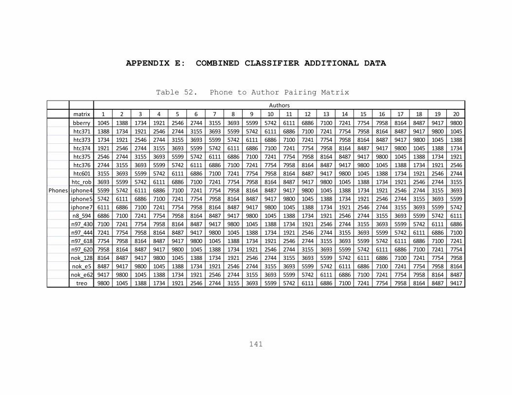
141
APPENDIX E: COMBINED CLASSIFIER ADDITIONAL DATA
Table 52. Phone to Author Pairing Matrix
matrix 1 2 3 4 5 6 7 8 9 10 11 12 13 14 15 16 17 18 19 20bberry 1045 1388 1734 1921 2546 2744 3155 3693 5599 5742 6111 6886 7100 7241 7754 7958 8164 8487 9417 9800htc371 1388 1734 1921 2546 2744 3155 3693 5599 5742 6111 6886 7100 7241 7754 7958 8164 8487 9417 9800 1045htc373 1734 1921 2546 2744 3155 3693 5599 5742 6111 6886 7100 7241 7754 7958 8164 8487 9417 9800 1045 1388htc374 1921 2546 2744 3155 3693 5599 5742 6111 6886 7100 7241 7754 7958 8164 8487 9417 9800 1045 1388 1734htc375 2546 2744 3155 3693 5599 5742 6111 6886 7100 7241 7754 7958 8164 8487 9417 9800 1045 1388 1734 1921htc376 2744 3155 3693 5599 5742 6111 6886 7100 7241 7754 7958 8164 8487 9417 9800 1045 1388 1734 1921 2546htc601 3155 3693 5599 5742 6111 6886 7100 7241 7754 7958 8164 8487 9417 9800 1045 1388 1734 1921 2546 2744htc_rob 3693 5599 5742 6111 6886 7100 7241 7754 7958 8164 8487 9417 9800 1045 1388 1734 1921 2546 2744 3155
Phones iphone4 5599 5742 6111 6886 7100 7241 7754 7958 8164 8487 9417 9800 1045 1388 1734 1921 2546 2744 3155 3693iphone5 5742 6111 6886 7100 7241 7754 7958 8164 8487 9417 9800 1045 1388 1734 1921 2546 2744 3155 3693 5599iphone7 6111 6886 7100 7241 7754 7958 8164 8487 9417 9800 1045 1388 1734 1921 2546 2744 3155 3693 5599 5742n8_594 6886 7100 7241 7754 7958 8164 8487 9417 9800 1045 1388 1734 1921 2546 2744 3155 3693 5599 5742 6111n97_430 7100 7241 7754 7958 8164 8487 9417 9800 1045 1388 1734 1921 2546 2744 3155 3693 5599 5742 6111 6886n97_444 7241 7754 7958 8164 8487 9417 9800 1045 1388 1734 1921 2546 2744 3155 3693 5599 5742 6111 6886 7100n97_618 7754 7958 8164 8487 9417 9800 1045 1388 1734 1921 2546 2744 3155 3693 5599 5742 6111 6886 7100 7241n97_620 7958 8164 8487 9417 9800 1045 1388 1734 1921 2546 2744 3155 3693 5599 5742 6111 6886 7100 7241 7754nok_128 8164 8487 9417 9800 1045 1388 1734 1921 2546 2744 3155 3693 5599 5742 6111 6886 7100 7241 7754 7958nok_e5 8487 9417 9800 1045 1388 1734 1921 2546 2744 3155 3693 5599 5742 6111 6886 7100 7241 7754 7958 8164nok_e62 9417 9800 1045 1388 1734 1921 2546 2744 3155 3693 5599 5742 6111 6886 7100 7241 7754 7958 8164 8487treo 9800 1045 1388 1734 1921 2546 2744 3155 3693 5599 5742 6111 6886 7100 7241 7754 7958 8164 8487 9417
Authors

142
Table 53. Confusion Matrix for Normalized Combined Classifier Matrix Pairing 1 Using 30 Tweets/Signal Vectors With One Tweet/Signal Vector per Training Set
label ‐>1045 1388 1734 1921 2546 2744 3155 3693 5599 5742 6111 6886 7100 7241 7754 7958 8164 8487 9417 9800
truth 1045 28 0 0 0 0 0 0 0 0 0 0 1 0 0 0 0 1 0 0 0| 1388 1 25 4 0 0 0 0 0 0 0 0 0 0 0 0 0 0 0 0 0v 1734 0 1 27 0 0 0 0 0 0 0 0 0 0 0 0 0 0 0 2 0
1921 0 0 0 25 0 4 0 0 0 0 0 0 0 0 0 0 0 0 1 02546 0 0 0 0 29 0 0 0 0 0 0 0 0 0 0 0 0 0 1 02744 1 1 0 4 0 23 0 0 0 0 0 0 0 0 0 0 0 0 1 03155 0 0 0 0 0 0 30 19 0 0 0 0 0 0 0 0 0 0 1 03693 0 0 0 0 0 0 0 10 0 0 0 0 0 0 0 0 0 0 0 05599 0 0 0 0 0 0 0 0 26 1 2 1 0 0 0 0 0 0 0 05742 0 0 0 0 0 0 0 0 7 23 0 0 0 0 0 0 0 0 0 06111 1 0 0 0 0 1 0 1 5 4 17 0 0 0 0 0 0 1 0 06886 0 0 0 0 0 0 0 0 0 0 0 30 0 0 0 0 0 0 0 07100 0 0 0 0 0 0 0 0 0 0 0 1 28 0 0 1 0 0 0 07241 0 1 0 0 0 0 0 0 0 0 1 2 1 25 0 0 0 0 0 07754 0 0 0 0 0 0 0 0 0 0 0 0 0 0 27 0 0 3 0 07958 0 0 0 0 0 0 0 0 0 0 0 1 5 1 0 23 0 0 0 08164 3 1 0 0 0 0 0 0 0 0 1 0 2 6 3 0 13 1 0 08487 0 0 0 0 0 0 0 0 0 0 0 0 0 0 2 0 0 28 0 09417 0 0 0 1 1 1 0 0 0 0 0 0 0 0 0 0 0 0 27 09800 0 0 0 0 1 0 0 0 0 0 0 0 0 0 0 0 0 0 0 29

143
Table 54. Confusion Matrix for Non-normalized Combined Classifier Matrix Pairing 1 Using 30 Tweets/Signal Vectors With One Tweet/Signal Vector per Training Set
label ‐>1045 1388 1734 1921 2546 2744 3155 3693 5599 5742 6111 6886 7100 7241 7754 7958 8164 8487 9417 9800
truth 1045 9 2 0 2 2 0 0 1 3 0 1 3 1 1 1 3 0 1 0 0| 1388 0 6 0 2 1 4 2 1 4 1 2 2 0 1 0 1 0 1 0 2v 1734 1 5 4 0 1 0 3 3 0 1 1 3 0 0 0 4 0 0 3 1
1921 0 5 3 4 1 4 5 0 0 0 0 0 1 2 1 3 0 1 0 02546 0 0 0 4 11 8 1 0 2 0 1 0 1 0 0 0 0 0 1 12744 0 2 1 2 4 10 0 0 3 1 1 0 1 0 0 1 0 1 2 13155 0 0 1 6 6 9 11 7 3 0 0 1 1 1 1 0 1 2 0 03693 0 0 0 1 1 0 0 7 0 0 0 0 0 0 0 0 1 0 0 05599 0 0 0 0 0 0 0 0 27 0 2 0 1 0 0 0 0 0 0 05742 3 1 1 0 1 0 4 0 4 10 1 1 1 0 0 1 0 0 2 06111 0 0 0 2 0 0 1 0 8 1 16 0 0 1 0 0 0 0 1 06886 0 2 0 0 1 1 2 0 2 0 1 17 1 0 0 2 1 0 0 07100 0 1 3 0 2 2 2 1 4 0 0 0 15 0 0 0 0 0 0 07241 0 1 0 0 2 1 5 0 3 0 4 2 0 10 0 2 0 0 0 07754 0 1 0 0 1 1 1 0 0 0 0 4 0 1 11 3 0 0 5 27958 0 1 2 1 0 1 3 0 0 1 1 1 2 1 0 14 0 0 2 08164 0 1 0 2 0 1 2 0 0 0 3 0 1 0 0 1 18 0 0 18487 1 2 0 2 2 0 1 1 3 0 1 0 0 0 1 1 0 15 0 09417 1 1 0 0 0 2 3 1 2 0 0 2 0 0 2 2 0 1 13 09800 0 0 0 1 4 2 1 0 0 0 2 1 3 0 0 0 1 1 0 14

144
Table 55. Confusion Matrix for Normalized Combined Classifier Matrix Pairing 1 Using 30 Tweets/Signal Vectors With Three Tweets/Signal Vectors per Training Set
label ‐>1045 1388 1734 1921 2546 2744 3155 3693 5599 5742 6111 6886 7100 7241 7754 7958 8164 8487 9417 9800
truth 1045 10 0 0 0 0 0 0 0 0 0 0 0 0 0 0 0 0 0 0 0| 1388 0 10 0 0 0 0 0 0 0 0 0 0 0 0 0 0 0 0 0 0v 1734 0 2 8 0 0 0 0 0 0 0 0 0 0 0 0 0 0 0 0 0
1921 0 0 0 7 0 3 0 0 0 0 0 0 0 0 0 0 0 0 0 02546 0 0 0 0 10 0 0 0 0 0 0 0 0 0 0 0 0 0 0 02744 0 0 0 1 0 9 0 0 0 0 0 0 0 0 0 0 0 0 0 03155 0 0 0 0 0 0 10 0 0 0 0 0 0 0 0 0 0 0 0 03693 0 0 0 0 0 0 0 10 0 0 0 0 0 0 0 0 0 0 0 05599 0 0 0 0 0 0 0 0 9 0 1 0 0 0 0 0 0 0 0 05742 0 0 0 0 0 0 0 0 1 9 0 0 0 0 0 0 0 0 0 06111 0 0 0 0 0 0 0 1 0 0 8 0 0 1 0 0 0 0 0 06886 0 0 0 0 0 0 0 0 0 0 1 10 1 0 0 0 0 0 0 07100 0 0 0 0 0 0 0 0 0 0 0 0 10 0 0 0 0 0 0 07241 0 0 0 0 0 0 0 0 0 0 0 1 0 8 0 0 1 0 0 07754 0 0 0 0 0 0 0 0 0 0 0 0 0 0 10 0 0 0 0 07958 0 0 0 0 0 0 0 0 0 0 0 0 1 0 0 9 0 0 0 08164 1 0 0 0 0 0 0 0 0 0 1 0 0 1 0 1 6 0 0 08487 0 0 0 0 0 0 0 0 0 0 0 0 0 0 2 0 0 8 0 09417 0 0 0 0 0 0 0 0 0 0 0 0 0 0 0 0 0 0 10 09800 0 0 0 0 0 0 0 0 0 0 0 0 0 0 0 0 0 0 1 10

145
Table 56. Confusion Matrix for Non-normalized Combined Classifier Matrix Pairing 1 Using 30 Tweets/Signal Vectors With Three Tweets/Signal Vectors per Training Set
label ‐>1045 1388 1734 1921 2546 2744 3155 3693 5599 5742 6111 6886 7100 7241 7754 7958 8164 8487 9417 9800
truth 1045 6 0 0 0 0 0 1 0 0 0 0 1 1 0 0 1 0 0 0 0| 1388 0 5 0 1 0 3 1 0 0 0 0 0 0 0 0 0 0 0 0 0v 1734 0 4 2 0 0 0 1 0 0 0 0 0 1 0 0 1 1 0 0 0
1921 0 4 1 0 0 3 2 0 0 0 0 0 0 0 0 0 0 0 0 02546 0 0 0 0 7 1 1 0 0 0 0 0 0 0 0 1 0 0 0 02744 0 2 0 1 2 5 0 0 0 0 0 0 0 0 0 0 0 0 0 03155 0 0 0 3 0 2 5 0 0 0 0 0 0 0 0 0 0 0 0 03693 0 0 0 0 1 0 0 6 3 0 0 0 0 0 0 0 0 0 0 05599 0 0 0 0 0 0 0 0 10 0 0 0 0 0 0 0 0 0 0 05742 0 0 1 0 0 1 2 0 2 4 0 0 0 0 0 0 0 0 0 06111 0 1 0 0 0 0 1 0 2 0 6 0 0 0 0 0 0 0 0 06886 0 1 0 0 1 1 1 0 0 0 0 6 0 0 0 0 0 0 0 07100 0 0 0 0 0 0 1 0 0 0 0 0 9 0 0 0 0 0 0 07241 0 0 0 0 0 0 0 0 1 0 0 2 0 6 0 1 0 0 0 07754 0 0 0 0 0 0 1 0 0 0 0 1 0 0 6 1 0 0 1 07958 0 0 0 0 0 0 0 0 0 0 0 0 1 0 0 9 0 0 0 08164 0 0 0 1 0 0 0 0 0 0 0 0 1 0 0 0 8 0 0 08487 0 0 0 0 0 0 0 0 1 0 0 0 0 0 0 0 0 9 0 09417 0 0 0 0 0 1 0 0 0 0 0 0 0 0 1 0 0 0 8 09800 0 0 0 1 2 0 0 0 0 0 1 0 2 0 0 0 0 0 0 4

146
Table 57. Confusion Matrix for Normalized Combined Classifier Matrix Pairing 1 Using 50 Tweets/Signal Vectors With One Tweet/Signal Vector per Training Set
label ‐>1045 1388 1734 1921 2546 2744 3155 3693 5599 5742 6111 6886 7100 7241 7754 7958 8164 8487 9417 9800
truth 1045 48 0 0 0 0 0 0 0 0 0 0 0 0 0 1 1 0 0 0 0| 1388 0 47 2 0 0 0 0 0 0 0 0 0 0 1 0 0 0 0 0 0v 1734 0 0 48 1 0 1 0 0 0 0 0 0 0 0 0 0 0 0 0 0
1921 0 0 0 43 0 8 0 0 0 0 0 0 0 0 0 0 0 0 0 02546 0 0 1 0 49 0 0 0 0 0 0 0 0 0 0 0 0 0 0 02744 1 0 1 13 1 31 1 0 0 0 0 0 0 0 0 0 0 0 2 03155 0 0 0 0 0 0 49 1 0 0 0 0 0 0 0 0 0 0 0 03693 0 1 0 0 0 0 0 48 0 0 0 0 0 0 0 0 0 0 1 05599 0 0 0 0 0 0 1 0 46 2 0 1 0 0 0 0 0 0 0 05742 0 0 0 0 0 0 0 0 6 40 4 0 0 0 0 0 0 0 0 06111 1 0 0 0 0 1 1 0 2 6 35 0 0 1 0 0 1 2 0 06886 0 0 0 0 0 0 0 0 0 0 1 48 0 0 0 1 0 0 0 07100 0 0 0 0 0 0 0 0 0 0 0 0 48 0 0 2 0 0 0 07241 0 0 0 0 0 0 0 0 0 0 0 2 1 46 0 0 1 0 0 07754 0 0 0 0 0 0 0 0 0 0 0 0 2 0 45 0 0 3 0 07958 0 0 0 0 0 0 0 0 0 0 0 0 5 1 0 44 0 0 0 08164 3 1 0 0 0 0 0 0 0 0 4 2 3 8 4 1 22 2 0 08487 0 0 0 0 0 0 1 0 0 0 0 0 0 0 2 0 0 47 0 09417 0 0 0 2 1 1 0 0 0 0 0 0 0 0 0 0 0 0 46 09800 0 0 0 0 0 0 0 0 0 0 0 0 0 0 0 0 0 0 0 50

147
Table 58. Confusion Matrix for Non-normalized Combined Classifier Matrix Pairing 1 Using 50 Tweets/Signal Vectors With One Tweet/Signal Vector per Training Set
label ‐>1045 1388 1734 1921 2546 2744 3155 3693 5599 5742 6111 6886 7100 7241 7754 7958 8164 8487 9417 9800
truth 1045 19 4 0 0 2 3 1 2 3 3 3 1 2 2 0 3 1 0 0 1| 1388 0 16 0 3 1 9 2 1 5 3 4 2 0 0 0 0 1 0 2 1v 1734 0 13 10 1 0 2 3 5 0 3 1 2 0 2 0 3 2 0 1 2
1921 1 15 4 14 0 8 1 0 1 1 2 0 0 0 0 1 1 0 2 02546 0 0 0 4 13 17 4 0 4 0 2 0 1 1 0 2 0 2 0 02744 0 2 1 3 14 20 0 0 2 1 2 1 2 0 0 0 0 0 1 13155 0 1 1 4 3 12 25 0 0 0 1 1 0 1 0 0 0 0 1 03693 0 0 0 0 4 1 5 24 3 0 1 3 0 0 1 0 3 3 1 15599 0 0 0 0 1 0 1 0 45 1 2 0 0 0 0 0 0 0 0 05742 3 4 0 0 2 3 3 2 2 20 2 3 3 1 1 0 0 0 1 06111 0 4 0 1 1 5 2 0 4 0 29 0 1 1 0 1 0 0 0 16886 1 5 0 0 1 2 1 0 1 3 2 23 2 0 0 8 0 0 1 07100 0 1 0 1 4 3 2 0 4 1 1 2 29 0 1 1 0 0 0 07241 0 4 0 1 2 1 2 0 3 1 4 2 0 26 0 1 2 0 0 17754 0 2 0 1 2 4 2 0 0 2 0 2 4 0 27 0 1 1 2 07958 0 2 0 1 0 3 1 0 0 0 2 7 2 3 1 28 0 0 0 08164 0 6 0 0 0 2 0 0 2 1 5 2 2 2 0 0 23 2 2 18487 1 2 0 0 1 3 4 1 4 0 3 0 0 0 2 0 0 28 0 19417 1 5 2 4 2 1 1 3 1 2 0 0 2 0 1 0 0 0 25 09800 0 1 0 2 11 2 2 0 2 0 3 1 3 0 0 0 0 0 0 23

148
Table 59. Confusion Matrix for Normalized Combined Classifier Matrix Pairing 1 Using 50 Tweets/Signal Vectors With Three Tweets/Signal Vectors per Training Set
label ‐>1045 1388 1734 1921 2546 2744 3155 3693 5599 5742 6111 6886 7100 7241 7754 7958 8164 8487 9417 9800
truth 1045 16 0 0 0 0 0 0 0 0 0 0 0 0 0 1 0 0 0 0 0| 1388 0 17 0 0 0 0 0 0 0 0 0 0 0 0 0 0 0 0 0 0v 1734 0 0 17 0 0 0 0 0 0 0 0 0 0 0 0 0 0 0 0 0
1921 0 0 0 16 0 1 0 0 0 0 0 0 0 0 0 0 0 0 0 02546 0 0 0 0 17 0 0 0 0 0 0 0 0 0 0 0 0 0 0 02744 0 0 0 2 0 15 0 0 0 0 0 0 0 0 0 0 0 0 0 03155 0 0 0 0 0 0 17 0 0 0 0 0 0 0 0 0 0 0 0 03693 0 0 0 0 0 0 0 17 0 0 0 0 0 0 0 0 0 0 0 05599 0 0 0 0 0 0 0 0 17 0 0 0 0 0 0 0 0 0 0 05742 0 0 0 0 0 0 0 0 1 16 0 0 0 0 0 0 0 0 0 06111 0 0 0 0 0 0 0 0 0 3 12 0 0 1 0 0 1 0 0 06886 0 0 0 0 0 0 0 0 0 0 0 16 0 0 0 1 0 0 0 07100 0 0 0 0 0 0 0 0 0 0 0 0 17 0 0 0 0 0 0 07241 0 0 0 0 0 0 0 0 0 0 0 0 0 17 0 0 0 0 0 07754 0 0 0 0 0 0 0 0 0 0 0 0 0 0 17 0 0 0 0 07958 0 0 0 0 0 0 0 0 0 0 0 0 2 0 0 15 0 0 0 08164 0 0 0 0 0 0 0 0 0 0 4 0 0 1 0 0 12 0 0 08487 0 0 0 0 0 0 0 0 0 0 0 0 0 0 0 0 0 17 0 09417 0 0 0 0 0 0 0 0 0 0 0 0 0 0 0 0 0 0 17 09800 0 0 0 0 0 0 0 0 0 0 0 0 0 0 0 0 0 0 0 17

149
Table 60. Confusion Matrix for Non-normalized Combined Classifier Matrix Pairing 1 Using 50 Tweets/Signal Vectors With Three Tweets/Signal Vectors per Training Set
label ‐>1045 1388 1734 1921 2546 2744 3155 3693 5599 5742 6111 6886 7100 7241 7754 7958 8164 8487 9417 9800
truth 1045 12 1 0 0 0 1 1 0 0 1 1 0 0 0 0 0 0 0 0 0| 1388 0 16 0 0 0 1 0 0 0 0 0 0 0 0 0 0 0 0 0 0v 1734 0 2 8 0 0 3 1 0 0 1 0 0 0 0 1 1 0 0 0 0
1921 0 0 0 12 0 4 1 0 0 0 0 0 0 0 0 0 0 0 0 02546 0 0 0 0 16 0 0 0 0 0 0 0 0 0 0 1 0 0 0 02744 0 1 0 1 0 14 0 0 0 0 0 0 1 0 0 0 0 0 0 03155 0 0 0 1 0 0 16 0 0 0 0 0 0 0 0 0 0 0 0 03693 0 0 0 0 1 0 0 15 1 0 0 0 0 0 0 0 0 0 0 05599 0 0 0 0 0 0 0 0 17 0 0 0 0 0 0 0 0 0 0 05742 0 1 1 1 0 2 0 0 1 11 0 0 0 0 0 0 0 0 0 06111 0 0 0 2 0 1 1 0 1 0 12 0 0 0 0 0 0 0 0 06886 0 3 0 0 1 0 0 0 1 0 0 8 1 0 0 2 0 0 1 07100 0 0 0 0 0 1 0 0 0 0 0 0 16 0 0 0 0 0 0 07241 0 1 0 0 1 2 0 0 1 0 0 0 0 10 0 1 1 0 0 07754 2 0 0 0 2 1 0 0 0 1 0 1 0 0 10 0 0 0 0 07958 1 0 0 1 0 1 0 0 0 0 0 2 0 0 0 12 0 0 0 08164 0 3 0 0 0 0 0 0 1 0 2 1 0 0 1 0 9 0 0 08487 0 1 0 0 1 0 0 0 0 0 0 0 0 0 1 0 0 14 0 09417 0 0 0 1 1 1 0 0 0 0 0 1 0 0 0 0 0 0 13 09800 0 0 0 1 4 0 0 0 0 0 1 0 1 0 0 0 0 0 0 10

150
Table 61. Confusion Matrix for Normalized Combined Classifier Matrix Pairing 1 Using 120 Tweets/Signal Vectors With One Tweet/Signal Vector per Training Set
label ‐>1045 1388 1734 1921 2546 2744 3155 3693 5599 5742 6111 6886 7100 7241 7754 7958 8164 8487 9417 9800
truth 1045 118 0 0 0 0 0 0 0 0 0 0 0 0 0 0 0 2 0 0 0| 1388 1 113 5 0 0 0 0 0 0 0 0 0 0 0 0 0 0 1 0 0v 1734 0 0 120 0 0 0 0 0 0 0 0 0 0 0 0 0 0 0 0 0
1921 0 0 0 111 0 8 0 0 0 0 0 0 0 0 0 0 0 0 1 02546 0 0 0 0 119 1 0 0 0 0 0 0 0 0 0 0 0 0 0 02744 1 0 0 26 0 91 0 0 0 0 0 0 0 0 0 0 0 0 2 03155 0 0 0 1 0 0 119 0 0 0 0 0 0 0 0 0 0 0 0 03693 0 0 0 0 0 0 0 120 0 0 0 0 0 0 0 0 0 0 0 05599 0 0 0 0 0 0 1 0 115 3 1 0 0 0 0 0 0 0 0 05742 0 0 0 0 0 0 0 0 7 106 7 0 0 0 0 0 0 0 0 06111 0 0 0 0 0 0 1 0 4 8 102 0 0 1 0 0 2 2 0 06886 0 0 0 0 0 0 0 0 0 0 0 118 1 0 0 1 0 0 0 07100 0 0 0 0 0 0 0 0 0 0 0 0 118 0 0 2 0 0 0 07241 0 0 0 0 0 0 0 0 0 0 0 0 1 114 0 1 4 0 0 07754 0 0 0 0 0 0 0 0 0 0 0 0 0 0 117 0 0 3 0 07958 0 0 0 0 0 0 0 0 0 0 0 0 5 1 0 114 0 0 0 08164 12 1 0 0 0 0 1 0 0 0 3 0 1 13 9 1 78 1 0 08487 0 0 0 0 0 1 0 0 0 0 0 0 0 0 0 0 0 119 0 09417 0 0 0 1 2 0 0 0 0 0 0 0 0 0 0 0 0 0 117 09800 0 0 0 0 0 0 0 0 0 0 0 0 0 0 0 0 0 0 0 120
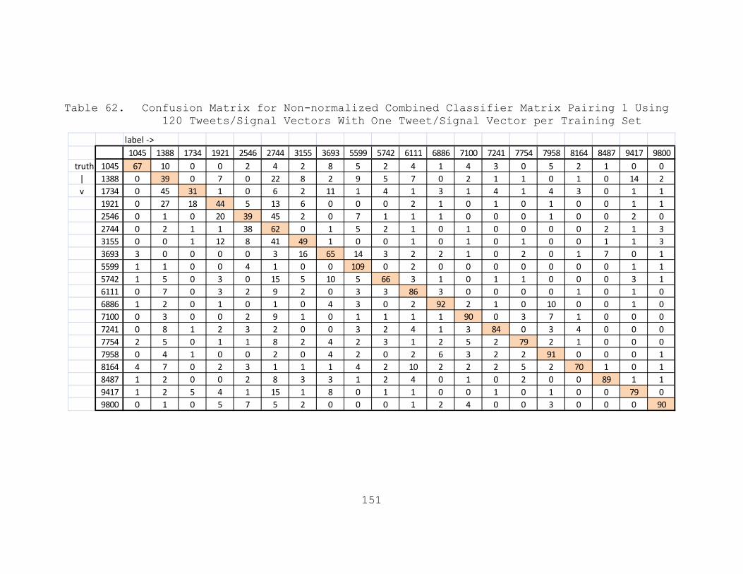
151
Table 62. Confusion Matrix for Non-normalized Combined Classifier Matrix Pairing 1 Using 120 Tweets/Signal Vectors With One Tweet/Signal Vector per Training Set
label ‐>1045 1388 1734 1921 2546 2744 3155 3693 5599 5742 6111 6886 7100 7241 7754 7958 8164 8487 9417 9800
truth 1045 67 10 0 0 2 4 2 8 5 2 4 1 4 3 0 5 2 1 0 0| 1388 0 39 0 7 0 22 8 2 9 5 7 0 2 1 1 0 1 0 14 2v 1734 0 45 31 1 0 6 2 11 1 4 1 3 1 4 1 4 3 0 1 1
1921 0 27 18 44 5 13 6 0 0 0 2 1 0 1 0 1 0 0 1 12546 0 1 0 20 39 45 2 0 7 1 1 1 0 0 0 1 0 0 2 02744 0 2 1 1 38 62 0 1 5 2 1 0 1 0 0 0 0 2 1 33155 0 0 1 12 8 41 49 1 0 0 1 0 1 0 1 0 0 1 1 33693 3 0 0 0 0 3 16 65 14 3 2 2 1 0 2 0 1 7 0 15599 1 1 0 0 4 1 0 0 109 0 2 0 0 0 0 0 0 0 1 15742 1 5 0 3 0 15 5 10 5 66 3 1 0 1 1 0 0 0 3 16111 0 7 0 3 2 9 2 0 3 3 86 3 0 0 0 0 1 0 1 06886 1 2 0 1 0 1 0 4 3 0 2 92 2 1 0 10 0 0 1 07100 0 3 0 0 2 9 1 0 1 1 1 1 90 0 3 7 1 0 0 07241 0 8 1 2 3 2 0 0 3 2 4 1 3 84 0 3 4 0 0 07754 2 5 0 1 1 8 2 4 2 3 1 2 5 2 79 2 1 0 0 07958 0 4 1 0 0 2 0 4 2 0 2 6 3 2 2 91 0 0 0 18164 4 7 0 2 3 1 1 1 4 2 10 2 2 2 5 2 70 1 0 18487 1 2 0 0 2 8 3 3 1 2 4 0 1 0 2 0 0 89 1 19417 1 2 5 4 1 15 1 8 0 1 1 0 0 1 0 1 0 0 79 09800 0 1 0 5 7 5 2 0 0 0 1 2 4 0 0 3 0 0 0 90

152
Table 63. Confusion Matrix for Normalized Combined Classifier Matrix Pairing 1 Using 120 Tweets/Signal Vectors With Three Tweets/Signal Vectors per Training Set
label ‐>1045 1388 1734 1921 2546 2744 3155 3693 5599 5742 6111 6886 7100 7241 7754 7958 8164 8487 9417 9800
truth 1045 40 0 0 0 0 0 0 0 0 0 0 0 0 0 0 0 0 0 0 0| 1388 0 40 0 0 0 0 0 0 0 0 0 0 0 0 0 0 0 0 0 0v 1734 0 0 40 0 0 0 0 0 0 0 0 0 0 0 0 0 0 0 0 0
1921 0 0 0 39 0 1 0 0 0 0 0 0 0 0 0 0 0 0 0 02546 0 0 0 0 40 0 0 0 0 0 0 0 0 0 0 0 0 0 0 02744 0 0 0 2 0 38 0 0 0 0 0 0 0 0 0 0 0 0 0 03155 0 0 0 0 0 0 40 0 0 0 0 0 0 0 0 0 0 0 0 03693 0 0 0 0 0 0 1 40 0 0 0 0 0 0 0 0 0 0 0 05599 0 0 0 0 0 0 0 0 40 0 0 0 0 0 0 0 0 0 0 05742 0 0 0 0 0 0 0 0 0 40 0 0 0 0 0 0 0 0 0 06111 0 0 0 0 0 0 0 0 0 2 38 0 0 0 0 0 0 0 0 06886 0 0 0 0 0 0 0 0 0 0 0 40 0 0 0 0 0 0 0 07100 0 0 0 0 0 0 0 0 0 0 0 0 40 0 0 0 0 0 0 07241 0 0 0 0 0 0 0 0 0 0 0 0 0 40 0 0 0 0 0 07754 0 0 0 0 0 0 0 0 0 0 0 0 0 0 40 0 0 0 0 07958 0 0 0 0 0 0 0 0 0 0 0 0 0 0 0 40 0 0 0 08164 0 0 0 0 0 0 0 0 0 0 0 0 0 0 0 0 40 0 0 08487 0 0 0 0 0 0 0 0 0 0 0 0 0 0 0 0 0 40 0 09417 0 0 0 0 0 0 0 0 0 0 0 0 0 0 0 0 0 0 40 09800 0 0 0 0 0 0 0 0 0 0 0 0 0 0 0 0 0 0 1 40

153
Table 64. Confusion Matrix for Non-normalized Combined Classifier Matrix Pairing 1 Using 120 Tweets/Signal Vectors With Three Tweets/Signal Vectors per Training Set
label ‐>1045 1388 1734 1921 2546 2744 3155 3693 5599 5742 6111 6886 7100 7241 7754 7958 8164 8487 9417 9800
truth 1045 36 1 0 0 0 1 0 0 0 0 0 0 1 0 0 1 0 0 0 0| 1388 0 25 0 0 0 11 0 0 0 1 0 0 0 0 0 0 0 0 3 0v 1734 1 22 15 0 0 0 1 0 0 1 0 0 0 0 0 0 0 0 0 0
1921 0 11 2 22 0 4 0 0 0 1 0 0 0 0 0 0 0 0 0 02546 0 0 0 2 19 18 0 0 1 0 0 0 0 0 0 0 0 0 0 02744 0 0 0 0 7 33 0 0 0 0 0 0 0 0 0 0 0 0 0 03155 0 0 0 2 2 15 20 0 0 0 0 0 0 0 1 0 0 0 0 03693 0 0 0 0 0 1 6 28 6 0 0 0 0 0 0 0 0 0 0 05599 0 0 0 0 0 0 0 0 40 0 0 0 0 0 0 0 0 0 0 05742 0 0 1 1 0 4 0 1 1 31 0 0 0 0 0 0 0 0 1 06111 0 0 0 0 0 2 1 0 0 0 37 0 0 0 0 0 0 0 0 06886 0 0 0 0 0 0 0 0 1 0 0 38 0 0 0 1 0 0 0 07100 0 0 0 0 0 0 0 0 0 0 0 0 40 0 0 0 0 0 0 07241 0 1 0 0 0 0 0 0 0 0 0 0 0 38 0 0 1 0 0 07754 0 1 0 0 0 2 0 0 0 0 0 0 0 0 37 0 0 0 0 07958 0 0 0 0 0 0 0 0 0 1 0 0 0 0 0 39 0 0 0 08164 0 2 0 0 0 0 0 1 1 0 2 0 0 0 0 0 34 0 0 08487 0 0 0 0 0 0 0 0 0 0 0 0 0 0 1 0 0 39 0 09417 0 0 0 1 0 1 0 0 0 1 0 0 0 0 0 0 0 0 37 09800 0 0 0 0 0 1 0 0 0 0 0 0 0 0 0 0 0 0 1 39

154
Table 65. Confusion Matrix for Normalized Combined Classifier Matrix Pairing 1 Using 120 Tweets/Signal Vectors With Five Tweets/Signal Vectors per Training Set
label ‐>1045 1388 1734 1921 2546 2744 3155 3693 5599 5742 6111 6886 7100 7241 7754 7958 8164 8487 9417 9800
truth 1045 22 1 0 0 0 0 0 0 1 0 0 0 0 0 0 0 0 0 0 0| 1388 0 24 0 0 0 0 0 0 0 0 0 0 0 0 0 0 0 0 0 0v 1734 0 1 21 0 0 1 1 0 0 0 0 0 0 0 0 0 0 0 0 0
1921 0 0 0 22 0 1 0 0 0 0 0 0 0 0 0 1 0 0 0 02546 0 0 0 0 24 0 0 0 0 0 0 0 0 0 0 0 0 0 0 02744 0 0 0 0 0 24 0 0 0 0 0 0 0 0 0 0 0 0 0 03155 0 0 0 0 0 0 24 0 0 0 0 0 0 0 0 0 0 0 0 03693 0 0 0 0 0 0 0 22 2 0 0 0 0 0 0 0 0 0 0 05599 0 0 0 0 0 0 0 0 24 0 0 0 0 0 0 0 0 0 0 05742 0 0 0 0 0 2 0 0 0 22 0 0 0 0 0 0 0 0 0 06111 0 0 0 0 0 0 0 0 0 0 24 0 0 0 0 0 0 0 0 06886 0 0 0 0 0 0 0 0 0 0 0 24 0 0 0 0 0 0 0 07100 0 0 0 0 0 0 0 0 0 0 0 0 24 0 0 0 0 0 0 07241 0 0 0 0 0 0 0 0 0 0 0 0 0 24 0 0 0 0 0 07754 0 0 0 0 0 0 0 0 0 0 0 0 0 0 24 0 0 0 0 07958 0 0 0 0 0 0 0 0 0 0 0 0 1 0 0 23 0 0 0 08164 0 0 0 0 0 0 0 1 0 0 1 0 0 0 0 0 22 0 0 08487 0 0 0 0 0 0 0 0 0 0 0 0 0 0 0 0 0 24 0 09417 0 0 0 0 0 0 0 0 0 0 0 0 0 0 0 0 0 0 24 09800 0 0 0 0 0 0 0 0 0 0 0 0 0 0 0 0 0 0 0 24
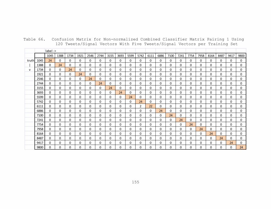
155
Table 66. Confusion Matrix for Non-normalized Combined Classifier Matrix Pairing 1 Using 120 Tweets/Signal Vectors With Five Tweets/Signal Vectors per Training Set
label ‐>1045 1388 1734 1921 2546 2744 3155 3693 5599 5742 6111 6886 7100 7241 7754 7958 8164 8487 9417 9800
truth 1045 24 0 0 0 0 0 0 0 0 0 0 0 0 0 0 0 0 0 0 0| 1388 0 24 0 0 0 0 0 0 0 0 0 0 0 0 0 0 0 0 0 0v 1734 0 0 24 0 0 0 0 0 0 0 0 0 0 0 0 0 0 0 0 0
1921 0 0 0 24 0 0 0 0 0 0 0 0 0 0 0 0 0 0 0 02546 0 0 0 0 24 0 0 0 0 0 0 0 0 0 0 0 0 0 0 02744 0 0 0 0 0 24 0 0 0 0 0 0 0 0 0 0 0 0 0 03155 0 0 0 0 0 0 24 0 0 0 0 0 0 0 0 0 0 0 0 03693 0 0 0 0 0 0 0 24 0 0 0 0 0 0 0 0 0 0 0 05599 0 0 0 0 0 0 0 0 24 0 0 0 0 0 0 0 0 0 0 05742 0 0 0 0 0 0 0 0 0 24 0 0 0 0 0 0 0 0 0 06111 0 0 0 0 0 0 0 0 0 2 22 0 0 0 0 0 0 0 0 06886 0 0 0 0 0 0 0 0 0 0 0 24 0 0 0 0 0 0 0 07100 0 0 0 0 0 0 0 0 0 0 0 0 24 0 0 0 0 0 0 07241 0 0 0 0 0 0 0 0 0 0 0 0 0 24 0 0 0 0 0 07754 0 0 0 0 0 0 0 0 0 0 0 0 0 0 24 0 0 0 0 07958 0 0 0 0 0 0 0 0 0 0 0 0 0 0 0 24 0 0 0 08164 0 0 0 0 0 0 0 0 0 0 0 0 0 0 0 0 24 0 0 08487 0 0 0 0 0 0 0 0 0 0 0 0 0 0 0 0 0 24 0 09417 0 0 0 0 0 0 0 0 0 0 0 0 0 0 0 0 0 0 24 09800 0 0 0 0 0 0 0 0 0 0 0 0 0 0 0 0 0 0 0 24
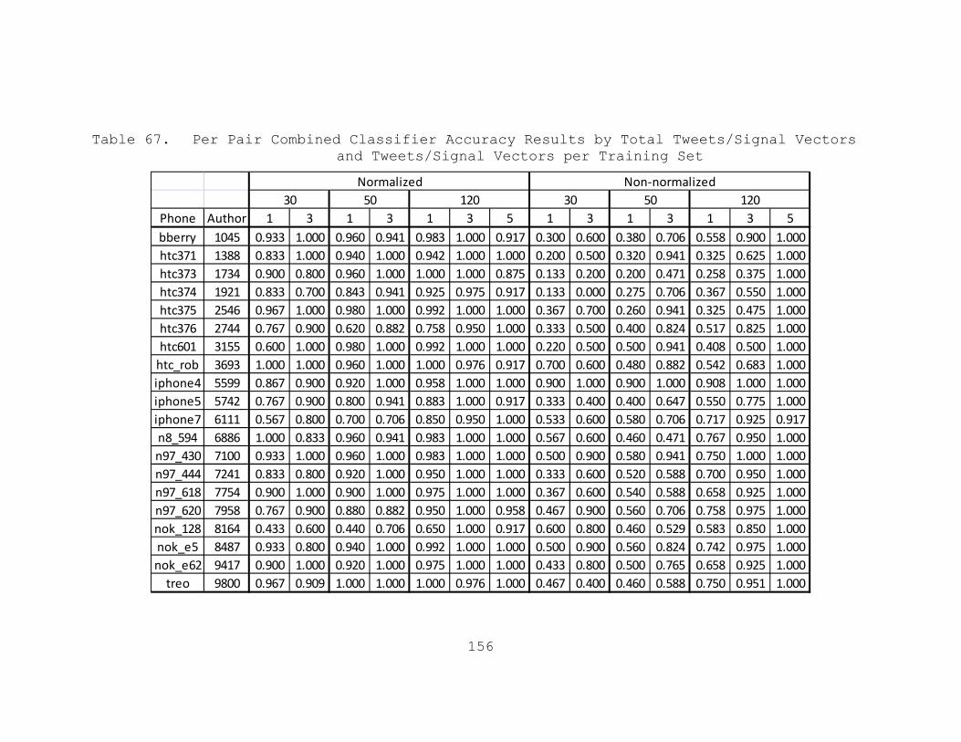
156
Table 67. Per Pair Combined Classifier Accuracy Results by Total Tweets/Signal Vectors and Tweets/Signal Vectors per Training Set
Phone Author 1 3 1 3 1 3 5 1 3 1 3 1 3 5bberry 1045 0.933 1.000 0.960 0.941 0.983 1.000 0.917 0.300 0.600 0.380 0.706 0.558 0.900 1.000htc371 1388 0.833 1.000 0.940 1.000 0.942 1.000 1.000 0.200 0.500 0.320 0.941 0.325 0.625 1.000htc373 1734 0.900 0.800 0.960 1.000 1.000 1.000 0.875 0.133 0.200 0.200 0.471 0.258 0.375 1.000htc374 1921 0.833 0.700 0.843 0.941 0.925 0.975 0.917 0.133 0.000 0.275 0.706 0.367 0.550 1.000htc375 2546 0.967 1.000 0.980 1.000 0.992 1.000 1.000 0.367 0.700 0.260 0.941 0.325 0.475 1.000htc376 2744 0.767 0.900 0.620 0.882 0.758 0.950 1.000 0.333 0.500 0.400 0.824 0.517 0.825 1.000htc601 3155 0.600 1.000 0.980 1.000 0.992 1.000 1.000 0.220 0.500 0.500 0.941 0.408 0.500 1.000htc_rob 3693 1.000 1.000 0.960 1.000 1.000 0.976 0.917 0.700 0.600 0.480 0.882 0.542 0.683 1.000iphone4 5599 0.867 0.900 0.920 1.000 0.958 1.000 1.000 0.900 1.000 0.900 1.000 0.908 1.000 1.000iphone5 5742 0.767 0.900 0.800 0.941 0.883 1.000 0.917 0.333 0.400 0.400 0.647 0.550 0.775 1.000iphone7 6111 0.567 0.800 0.700 0.706 0.850 0.950 1.000 0.533 0.600 0.580 0.706 0.717 0.925 0.917n8_594 6886 1.000 0.833 0.960 0.941 0.983 1.000 1.000 0.567 0.600 0.460 0.471 0.767 0.950 1.000n97_430 7100 0.933 1.000 0.960 1.000 0.983 1.000 1.000 0.500 0.900 0.580 0.941 0.750 1.000 1.000n97_444 7241 0.833 0.800 0.920 1.000 0.950 1.000 1.000 0.333 0.600 0.520 0.588 0.700 0.950 1.000n97_618 7754 0.900 1.000 0.900 1.000 0.975 1.000 1.000 0.367 0.600 0.540 0.588 0.658 0.925 1.000n97_620 7958 0.767 0.900 0.880 0.882 0.950 1.000 0.958 0.467 0.900 0.560 0.706 0.758 0.975 1.000nok_128 8164 0.433 0.600 0.440 0.706 0.650 1.000 0.917 0.600 0.800 0.460 0.529 0.583 0.850 1.000nok_e5 8487 0.933 0.800 0.940 1.000 0.992 1.000 1.000 0.500 0.900 0.560 0.824 0.742 0.975 1.000nok_e62 9417 0.900 1.000 0.920 1.000 0.975 1.000 1.000 0.433 0.800 0.500 0.765 0.658 0.925 1.000treo 9800 0.967 0.909 1.000 1.000 1.000 0.976 1.000 0.467 0.400 0.460 0.588 0.750 0.951 1.000
Normalized Non‐normalized30 50 120 30 50 120

157
Figure 51. Averaged Accuracy Results of Normalized Combined Classifiers for Each Phone-Author Pairing
Matrix Using One Tweet per Training Set
Figure 52. Averaged Accuracy Results of Normalized
Combined Classifiers for Each Phone-Author Pairing Matrix Using Three Tweets per Training Set

158
Figure 53. Averaged Accuracy Results of Non-Normalized
Combined Classifiers for Each Phone-Author Pairing Matrix Using One Tweet per Training Set
Figure 54. Averaged Accuracy Results of Non-Normalized
Combined Classifiers for Each Phone-Author Pairing Matrix Using Three Tweets per Training Set

159
LIST OF REFERENCES
[1] CTIA – The Wireless Association. Wireless Quick Facts, Mid-Year Figures. June 2010. [Online]. Available: http://www.ctia.org/advocacy/research/index.cfm/aid/10323 (accessed March 6, 2011).
[2] L. Castillo. Sale of SIM cards to be regulated and monitored. Mindanao Current 30 January 2011. [Online]. Available: http://themindanaocurrent.blogspot.com/2011/01/sale-of-sim-cards-to-be-regulated-and.html (accessed March 10, 2011).
[3] R. Layton, P. Watters and R. Dazeley, "Authorship Attribution for Twitter in 140 Characters or Less," in Cybercrime and Trustworthy Computing Workshop (CTC), 2010 Second, 2010, p. 1.
[4] V. Brik, S. Banerjee, M. Gruteser and S. Oh, "Wireless Device Identification with Radiometric Signatures," in MobiCom '08: Proceedings of the 14th ACM International Conference on Mobile Computing and Networking, San Francisco, California, USA, 2008, pp. 116-127.
[5] Twitter. About Twitter. 13 December 2010. [Online]. Available: https://twitter.com/about (accessed December 13, 2010).
[6] 3GPP TS 03.40, “Technical Realization of the Short Message Service (SMS) (Release 1998)”.
[7] D. Boyd, S. Golder, and G. Lotan, “Tweet, Tweet, Retweet: Conversational Aspects of Retweeting on Twitter,” in Proceedings of the 43rd Hawaii International Conference on System Sciences, Kauai, HI, January 6, 2010.
[8] IANA, “Uniform Resource Locators (URL)”, RFC 1738, December 1994.
[9] E. Stamatatos, "A survey of modern authorship attribution methods," Journal of the American Society for Information Science and Technology, vol. 60, pp. 538-556, March 2009.

160
[10] J. Lin, “Automatic Author Profiling of Online Chat Logs,” M.S. thesis, Naval Postgraduate School, Monterey, CA, 2007.
[11] V. Keselj, F. Peng, N. Cercone and C. Thomas, "N-gram-based Author Profiles for Authorship Attribution," In Proceedings of the Conference Pacific Association for Computational Linguistics, PACLING ’03, 2003, p. 255.
[12] G. Frantzeskou, E. Stamatatos, S. Gritzalis and S. Katsikas, "Effective Identification of Source Code Authors Using Byte-level Information," in Proceedings of the 28th International Conference on Software Engineering, Shanghai, China, 2006, pp. 893-896.
[13] L. E. Langley, "Specific Emitter Identification (SEI) and Classical Parameter Fusion Technology," in WESCON/'93. Conference Record, 1993, p. 377.
[14] B. Danev and S. Capkun, "Transient-based Identification of Wireless Sensor Nodes," in IPSN '09: Proceedings of the 2009 International Conference on Information Processing in Sensor Networks, 2009, pp. 25-36.
[15] A. Candore, O. Kocabas and F. Koushanfar, "Robust Stable Radiometric Fingerprinting for Wireless Devices," in IEEE International Workshop on Hardware-Oriented Security and Trust, 2009, HOST '09, 2009, p. 43.
[16] T. Kohno, A. Broido and K. C. Claffy, "Remote Physical Device Fingerprinting," IEEE Transactions on Dependable and Secure Computing, vol. 2, p. 93, April–June 2005.
[17] GSM World. Market Data Summary ~ GSM World. 15 December 2010. [Online]. Available: http://www.gsmworld.com/newsroom/market-data/market_data_summary.htm (accessed December 15, 2010).
[18] M. Rahnema, "Overview of the GSM System and Protocol Architecture," Communications Magazine, IEEE, vol. 31, p. 92, April 1993.

161
[19] Wikimedia Commons. File:Gsm structures.svg. 15 December 2010. [Online]. Available: https://secure.wikimedia.org/wikipedia/commons/wiki/File:Gsm_structures.svg (accessed December 15, 2010).
[20] C. Peersman, S. Cvetkovic, P. Griffiths and H. Spear, "The Global System for Mobile Communications Short Message Service," Personal Communications, IEEE, vol. 7, p. 15, June 2000.
[21] J. Scourias. "Overview of the Global System for Mobile Communications." December 15, 2010. [Online]. Available: http://ccnga.uwaterloo.ca/~jscouria/GSM/gsmreport.html (accessed December 15, 2010).
[22] K. Murota and K. Hirade, "GMSK Modulation for Digital Mobile Radio Telephony," IEEE Transactions on Communications, vol. 29, p. 1044, July 1981.
[23] T. Turletti, "GMSK in a nutshell," Technical Notes, Cambridge, MA, April 1996.
[24] D. Lewis, “Naïve (Bayes) at Forty: The Independence Assumption in Information Retrieval,” in Proceedings of the 10th European Conference on Machine Learning, ECML ’98, London, UK, 1998.
[25] E. Alpaydin, Introduction to Machine Learning. Cambridge, MA: MIT Press, 2004.
[26] D. Jurafsky and J. H. Martin, Speech and Language Processing: An Introduction to Natural Language Processing, Speech Recognition, and Computational Linguistics. Prentice-Hall, 2009.
[27] I. H. Witten and T. C. Bell, "The Zero-frequency Problem: Estimating the Probabilities of Novel Events in Adaptive Text Compression," IEEE Transactions on Information Theory, vol. 37, p. 1085, July 1991.
[28] J. Kittler, M. Hatef, R. P. W. Duin and J. Matas, "On Combining Classifiers," IEEE Transactions on Pattern Analysis and Machine Intelligence, vol. 20, p. 226, March 1998.

162
[29] L. Xu, A. Krzyzak, C. Y. Suen, “Methods of Combining Multiple Classifiers and Their Applications to Handwriting Recognition,” IEEE Transactions on Systems, Man, and Cybernetics, vol. 22, p. 418, May/June 1992.
[30] C. J. van Rijsbergen. Information. 1979. Retrieval. [Online]. Available: http://www.dcs.gla.ac.uk/Keith/Chapter.7/Ch.7.html (accessed December 17, 2010).
[31] Twitter Development. Streaming API Documentation. January 9, 2011. [Online]. Available: http://dev.twitter.com/pages/streaming_api (accessed January 9, 2011).
[32] A. Schein. The Naval Postgraduate School Machine Learning Library. Monterey, CA. 2010. [Online]. Available: http://sourceforge.net/projects/npsml/ [Accessed: January 15, 2011].
[33] 3GPP TS 05.05, “Radio Transmission and Reception (Release 1999)”.
[34] 3GPP TS 11.21, “Base Station System (BSS) equipment specification; Radio aspects (Release 1999)”.
[35] Agilent Technologies, “User’s Guide, Agilent Technologies 8922M/S GSM Test Set,” Agilent Part No. 08922-90211, January 1998.
[36] R. Honaker, “Novel Topic Authorship Attribution,” M.S. thesis, Naval Postgraduate School, Monterey, CA, 2011.
[37] P. Kimuli, ”Introduction to GSM and GSM mobile RF transceiver derivation,” RF Design, June 2003.
[38] Agilent Technologies, “Understanding GSM/EDGE Transmitter and Receiver Measurements for Base Transceiver Stations and their Components,” Application Note 1312, August 24, 2008.

163
INITIAL DISTRIBUTION LIST
1. Defense Technical Information Center Ft. Belvoir, Virginia
2. Dudley Knox Library Naval Postgraduate School Monterey, California
3. Dr. Robert Beverly Naval Postgraduate School Monterey, California 4. Dr. Craig Martell Naval Postgraduate School Monterey, California 5. Sarah Boutwell Naval Postgraduate School Monterey, California