------------

Tel. +01-859-2573171. E-mail address: hayes@cs.uky.edu

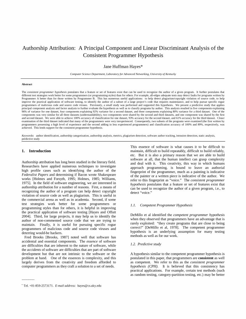
Authorship Attribution: A Principal Component and Linear Discriminant Analysis of the Consistent Programmer Hypothesis

Jane Huffman Hayes*

Computer Science Department, Laboratory for Advanced Networking, University of Kentucky

Abstract

The consistent programmer hypothesis postulates that a feature or set of features exist that can be used to recognize the author of a given program. It further postulates that different test strategies work better for some programmers (or programming styles) than for others. For example, all-edges adequate tests may detect faults for programs written by Programmer A better than for those written by Programmer B. This has numerous useful applications: to help detect plagiarism/copyright violation of source code, to help improve the practical application of software testing, to identify the author of a subset of a large project’s code that requires maintenance, and to help pursue specific rogue programmers of malicious code and source code viruses. Previously, a small study was performed and supported this hypothesis. We present a predictive study that applies principal component analysis and factor analysis to further evaluate the hypothesis as well as to classify programs by author. This analysis resulted in five components explaining 96% of variance for one dataset, four components explaining 92% variance for a second dataset, and three components explaining 80% variance for a third dataset. One of the components was very similar for all three datasets (understandability), two components were shared by the second and third datasets, and one component was shared by the first and second dataset. We were able to achieve 100% accuracy of classification for one dataset, 93% accuracy for the second dataset, and 61% accuracy for the third dataset. Closer examination of the third dataset indicated that many of the programmers were very inexperienced. Consequently, two subsets of the programs were examined (the first written by programmers possessing a high level of experience and the second adding in less experienced programmers) and classification accuracy of 100% and 89%, respectively, was achieved. This lends support for the consistent programmer hypothesis.

Keywords: author identification, authorship categorization, authorship analysis, metrics, plagiarism detection, software author tracking, intrusion detection, static analysis, predictive study

1. Introduction

Authorship attribution has long been studied in the literary field. Researchers have applied numerous techniques to investigate high profile cases such as identifying the author of the Federalist Papers and determining if Bacon wrote Shakespeare works [Holmes and Forsyth, 1995; Holmes, 1985; Williams, 1975]. In the field of software engineering, we are interested in authorship attribution for a number of reasons. First, a means of recognizing the author of a program can help detect copyright violation of source code as well as plagiarism. This is useful in the commercial arena as well as in academia. Second, if some test strategies work better for some programmers or programming styles than for others, it is helpful in improving the practical application of software testing [Hayes and Offutt 2004]. Third, for large projects, it may help us to identify the author of non-commented source code that we are trying to maintain. Finally, it is useful for pursuing specific rogue programmers of malicious code and source code viruses and deterring would-be hackers. Fred Brooks [Brooks, 1987] noted well that software has accidental and essential components. The essence of software are difficulties that are inherent to the nature of software, while the accidents of software are difficulties that are part of software development but that are not intrinsic to the software or the problem at hand. One of the essences is complexity, and this largely derives from the creativity and freedom afforded to computer programmers as they craft a solution to a set of needs.

This essence of software is what causes it to be difficult to maintain, difficult to build repeatably, difficult to build reliably, etc. But it is also a primary reason that we are able to build software at all, that the human intellect can grasp complexity and deal with it. This creativity, this way in which humans approach programming, is bound to leave an authorial fingerprint of the programmer, much as a painting is indicative of the painter or a written piece is indicative of the author. We refer to this fingerprint as “voice.” The consistent programmer hypothesis postulates that a feature or set of features exist that can be used to recognize the author of a given program, i.e., to detect “voice.”

1.1. Competent Programmer Hypothesis

DeMillo et al identified the competent programmer hypothesiswhen they observed that programmers have an advantage that is rarely exploited: “they create programs that are close to being correct!” [DeMillo et al, 1978]. The competent programmer hypothesis is an underlying assumption for many testing methods as well as for our work.

1.2. Predictive study

A hypothesis similar to the competent programmer hypothesis is postulated in this paper, that programmers are consistent as well as competent. We refer to this as the consistent programmer hypothesis (CPH). It is believed that this consistency has practical applications. For example, certain test methods (such as random testing, category-partition testing, etc.) may be better

2

suited to one programmer than to others. The goal of this study is to evaluate the static features (if any) that can be used to recognize the author of a given program. A correlational study seeks to discover relationships between variables, but cannot determine “cause.” There are several types of correlational studies. A predictive study was the appropriate choice for this work. Predictive correlational studies attempt to predict the value of a criterion variable from a predictor variable using the degree of relationship between the variables. We are using author identity (known) as the criterion variable and a discriminator comprised of static features as the predictor variable. A study of the CPH was previously undertaken (Analysis of Variance (ANOVA) was applied to the data) and indicated support for the general hypothesis but not for the testing hypothesis [Hayes and Offutt, 2004]. The current predictive study further evaluates the consistent programmer hypothesis as well as uses the linear discriminant to classify computer programs according to author. Three datasets were examined using two techniques in parallel, ANOVA and principal component analysis with linear discriminant analysis. Analysis of variance was performed on all datasets. The features were then subjected to PCA. The reduced components were rotated as described in Section 4.5. We then applied LDA on the component metrics obtained from the PCA. To develop the classification criterion, we used a linear method that fits a multivariate normal density to each group, with a pooled estimate of covariance [The MathWorks, Inc., 2002].

1.3. Paper organization

In Section 2, related work and the consistent programmer hypothesis are discussed. Section 3 describes the research hypothesis. Section 4 defines the design of the predictive study. The techniques used, the subject programs evaluated, and the measurements taken for these subject programs are presented. Section 5 addresses the results of the study. Finally, Section 6 discusses future work.

2. Related work

Related work in the area of authorship identification is presented. First, work in the literary field is discussed. Next, software forensics is presented. The use of software measures for prediction and/or classification follows. Finally, the CPH and the unique contributions of the paper are presented.

2.1. Literary authorship attribution

As stated in the introduction, research has been performed, dating back to the early 1900s, to determine the authors of literary works. In general, researchers determine features of interest in literary works that they hypothesize can be used to recognize authors. Some researchers use style markers such as punctuation marks, average word length, average sentence length, or non-lexical style markers such as sentence and chunk boundaries [Stamatatos et al, 2001]. Other researchers use features such as n-grams (e.g., bi-grams (groupings of two words), tri-grams (grouping of three words), etc.). Once the features of interest have been determined, researchers apply

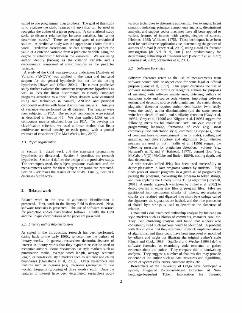
various techniques to determine authorship. For example, latent semantic indexing, principal components analysis, discriminant analysis, and support vector machines have all been applied to various features of interest with varying degrees of success [Holmes, 1985; Williams, 1975]. These techniques have been used for such diverse applications as: determining the gender of authors of e-mail [Corney et al, 2002], using e-mail for forensic investigation [de Vel et al, 2001], and predominantly for determining authorship of free-form text [Soboroff et al, 1997; Baayen et al, 2002; Stamatatos et al, 2001].

2.2. Software Forensics

Software forensics refers to the use of measurements from software source code or object code for some legal or official purpose [Gray et al, 1997]. Our paper discusses the use of software measures to profile or recognize authors for purposes of assisting with software maintenance, deterring authors of malicious code and source code viruses, improving software testing, and detecting source code plagiarism. As stated above, plagiarism detection requires author identification (who really wrote the code), author discrimination (did the same person write both pieces of code), and similarity detection [Gray et al, 1998]. Gray et al. [1998] and Kilgour et al. [1998] suggest the following measures for malicious code analysis: choice of programming language, formatting of code (e.g., most commonly used indentation style), commenting style (e.g., ratio of comment lines to non-comment lines of code), spelling and grammar, and data structure and algorithms (e.g., whether pointers are used or not). Sallis et al. [1996] suggest the following measures for plagiarism detection: volume (e.g., Halstead’s n, N, and V [Halstead, 1977]), control flow (e.g., McCabe’s V(G) [McCabe and Butler, 1989]), nesting depth, and data dependency. A web service called JPlag has been used successfully to detect plagiarism in Java programs written by students. JPlag finds pairs of similar programs in a given set of programs by parsing the programs, converting the program to token strings, and then applying the Greedy String Tiling algorithm [Prechelt, 2001]. A similar approach was taken by Finkel et al [2002] to detect overlap in either text files or program files. Files are partitioned into contiguous chunks of tokens, representative chunks are retained and digested into short byte strings called the signature, the signatures are hashed, and then the proportion of shared byte strings is used to determine the closeness of relation. Oman and Cook examined authorship analysis by focusing on style markers such as blocks of comments, character case, etc. They used clustering analysis and found that authors who consistently used such markers could be identified. A problem with this study is that they examined textbook implementations of algorithms, and these could have been improved or modified by editors and might not illustrate the original author’s style [Oman and Cook, 1989]. Spafford and Weeber [1993] define software forensics as examining code remnants to gather evidence about the author. They compare this to handwriting analysis. They suggest a number of features that may provide evidence of the author such as data structures and algorithms, choice of system calls, errors, comment styles, etc. Researchers at the University of Otago have developed a system, Integrated Dictionary-based Extraction of Non-language-dependent Token Information for Forensic

3

Identification, Examination, and Discrimination (IDENTIFIED), to extract counts of metrics and user defined meta-metrics to support authorship analysis [Gray et al, 1998]. In a later paper [MacDonell et al, 1999], these researchers examined the usefulness of feed-forward neural networks (FFNN), multiple discriminant analysis (MDA), and case-based reasoning (CBR) for authorship identification. The data set included C++ programs from seven authors (source code for three authors came from programming books, source code for one author was from examples provided with a C++ compiler, and three authors were experienced commercial programmers). Twenty-six measures were extracted (using IDENTIFIED) including proportion of blank lines, proportion of operators with whitespace on both sides, proportion of operators with whitespace on left side, proportion of operator with whitespace on right side, and the number of while statements per non-comment lines of code. All three techniques provided authorship identification accuracy between 81.1% and 88% on a holdout testing set, with CBR outperforming the other models in all cases (by 5 – 7%) [MacDonell et al, 1999]. Kilgour et al. [1998] looked at the usefulness of fuzzy logic variables for authorship identification. The data set was comprised of eight C++ programs written by two textbook authors. Two experienced software developers then subjectively analyzed the programs, examined measures such as spelling errors, whether the comments matched the code, and meaningful identifiers. They then assigned one of the fuzzy values Never, Occasionally, Sometimes, Most of the Time, and Always to each measure. The authors concluded that fuzzy-logic linguistic variables have promise for improving the accuracy and ease of authorship analysis models [Kilgour et al, 1998]. Collberg and Thomborson [2000] examined methods for defending against various security attacks. They suggested using code obfuscation to transform a program into one that is more difficult to reverse engineer, while maintaining the semantics of the program. It appears that control and data transformations might hold promise for erasing a programmer's "style," though not all factors being explored for the CPH would be "erased." Also, the lexical transformation they presented [Collberg and Thomborson, 2000] would not serve to remove the programmer's signature.

2.3. Classification using software measures

The development of predictive code quality models is a very active research area. This area is of interest to us because software measures are used to build predictive models. The main difference is that our model predicts authorship whereas the models described here predict code quality. Nikora and Munson applied principal component analysis to 12 correlated metrics to extract uncorrelated sources of variation for building fault predictors [Nikora and Munson, 2003]. The three new components accounted for 85% of the variation in the 12 metrics, with the largest component, control flow, accounting for 40% of the variation. Their resulting regression model was able to account for 60% of the variation in the cumulative fault count for a NASA Mission Data System. Munson and Koshgoftaar [1992] used 14 code metrics to discriminate between programs with less than five faults and those having more than five faults. They applied discriminant analysis with principal components to two applications. For the second application, they found two components of interest, one related to size and one related to control flow. Their model was able to

classify 75% of the modules of the first application and 62% of those of the second application (with a high level of confidence) with respective Type II error rates of only 4% and 1%. Briand, Melo, and Wust [2002] were interested in whether a design metric-based model built for one object-oriented system could be used for other systems. They built a general, tailorable cost-benefit model using a regression-based technique called Multivariate Adaptive Regression Splines (MARS). They also applied PCA to a set of metrics and found that six components captured 76% of the dataset variance, with class size component accounting for 33% of the variance. They found that the MARS system was more complete than a linear logistic regression model. That is, MARS was more accurate for classes containing larger numbers of faults. Briand, Basili, and Hetmanski [1993] also predicted fault prone components by applying Optimized Set Reduction, classification tree, and two logistic regression models to design and code metrics of a 260,000 line of code system. They found the OSR classifications to be the most complete and correct (classified components correctly) at 96% and 92% respectively. Another classification work addresses software reuse and its potential for success [Rothenberger et al, 2003]. The researchers surveyed 71 development groups on their reuse practices. Using pca, they developed six dimensions (or components), with Planning and Improvement accounting for the largest portion of the variance at 24.9%. They then showed that these components cluster into five distinct reuse strategies, with different potentials for reuse success. Lanubile and Vissaggio [1995, 1997] took a slightly different approach to the predictive quality model problem. Again they were interested in building models to predict high-risk, fault prone components. But they decided to study the various modeling techniques available to build such models. They studied pca, discriminant analysis, logistic regression, logical classification models, layered neural networks, and holographic networks. They used data from 27 Pascal student projects and examined 11 complexity measures such as Halstead’s N2, Halstead’s V, McCabe’s v(G), etc. [Halstead 1977; McCabe and Butler, 1989]. They found that models built with pca followed by either discriminant analysis or logistic regression had the highest quality values (completeness of 68% and 74% respectively), but required the inspection of a great majority of the components (wasted inspection of 55 and 56% respectively).

2.4. The Consistent Programmer Hypothesis

Hayes and Offutt posited the consistent programmer hypothesis [Hayes and Offutt, 2004]. They applied ANOVA to the static and dynamic features of two datasets. The dynamic features examined the probability that a given code location might be able to “hide” a code defect. A commercial tool was used to collect dynamic features. The first, small dataset consisted of three programs written by five programmers (total of 15 programs). Each programmer was given the same specifications for the three programs. ANOVA showed that five static features have potential for recognizing the author of a program: number of lint warnings, number of unique constructs, number of unique operands, average occurrence of operators, and average occurrence of constructs [Hayes and Offutt, 2004]. Three of these features indicated statistical significance for both individual programmers and the application. Also, the ANOVA showed no evidence of a difference among programmers for two simple programs - Mid and Trityp. For example, the p-value for average occurrence of operands was 0.35. However, there was a

4

statistically significant difference (p-value less than 0.05) between the programmers for the more complicated program Find. This makes sense because Find seemed to be the most difficult of the three programs for all programmers. The initial belief that only experienced programmers would exhibit style can perhaps be broadened to include the writing of complicated or non-trivial programs. That is, experienced programmers preparing non-trivial applications are both prerequisites to detecting consistency and “voice” in a program. The second dataset consisted of four networking programs written by 15 graduate students (total of 60 programs). The features were generated using a commercial tool, and hence were not all comparable to the features from the first dataset1. ANOVA showed that the static feature number of comments per program line has potential for recognizing the author of a program. A discriminator was built by combining the average occurrence of operands, the average occurrence of operators, and the average occurrence of constructs. The discriminator produced a range of values for each of the programmers, i.e., a look-up table. For a new program written by one of the five programmers, static analysis would be performed and the discriminator value calculated. The value for the new program should fall in the range for that programmer and for no other programmer. The generated discriminator ranges were not overlapping. However, the results cannot be generalized without examining additional programs written by the same programmers. Also, the discriminator needs to be applied to a larger dataset. We refer to this work by Hayes and Offutt as the Hayes-Offutt study.

2.5. Contributions

Our approach differs from those discussed in sections 2.1 – 2.3 in several ways. First, we emphasize structural measures instead of stylistic measures. When attempting to mask identity, an author can easily modify stylistic items within a program. Stylistic measures such as blank lines, indentation, in-line comments, use of upper or lower case for variable names, etc. are then no longer reliable. This approach to masking is often seen when multiple students have copied from one student’s program. The plagiarizing students re-name all the variables. They remove or modify the comments and blank space. They re-order the methods or procedures. They modify indentation. Also, stylistic features may be omitted from source code whereas programmers must use structural constructs to write functioning code. Second, our approach does not require large quantities of data (such as is needed to train a FFNN). Third, we use measures derived from dynamic analysis of the programs as well as measures derived from static analysis [Hayes and Offutt, 2004]. Fourth, we concentrate on classifying programs by author as opposed to classifying components as fault prone or not fault prone. Note that we are addressing a multiple classification problem, not a binary one. Finally, we performed a study to validate our research. For all datasets, we used programs developed by multiple authors according to the same written program specification. For one dataset, we used professional programmers. This helped control for confounding factors [Hayes and Offutt, 2004].

1 At the time of the earlier work, no single tool was available to meet our needs.

3. Research hypothesis

There are two aspects to this work: a general hypothesis related to the CPH, and an application of distinguishing features to assist in authorship attribution. Each is addressed below.

3.1. Study of Features for Authorship Attribution

The general hypothesis for this study is that one or more features exist for a program that can identify the author of the program. More specifically, the following are hypothesized:

1. The static measure of number of comments per program line is correlated with the individual programmer. The null hypothesis is that the mean value of number of comments per program line is not effected by programmer.

2. The static measure of average occurrence of operands is correlated with the individual programmer. The null hypothesis is that the mean value of average occurrence of operands is not effected by programmer.

3. The static measure of average occurrence of operators is correlated with the individual programmer. The null hypothesis is that the mean value of average occurrence of operators is not effected by programmer.

4. The static measure of number of unique operands iscorrelated with the individual programmer. The null hypothesis is that the mean value of number of unique operands is not effected by programmer.

5. A certain level of experience with a programming language and application domain is required in order for a programmer to exhibit voice.

Number of comments per program line should help distinguish programmers as the decision of how much documentation to include in-line is a highly personal one. In our courses at the University of Kentucky, we strongly encourage the graduate students to thoroughly comment their source code. However, we observe that there is a wide deviation of end results, further illustrating the personal nature of this measure. Average occurrence of operands and number of unique operands should also be distinguishing features. Programmers approach a problem solution from their own creative perspective. Some programmers will use significantly more operands to solve the same problem as another programmer. This applies to unique operands as well as total number of operands (hence impacting average occurrence of operands). Finally, programmers have personal preferences on the use of operators also. One programmer’s solution may require very few operators, another programmer may use many more. It is likely that none of these features will show much difference between programmers for small programs. But for programs of some size and complexity, we expect to see significant differences among programmers. Also, it is likely that these features will not show much difference between inexperienced programmers (lack experience with a programming language or application domain). In this study, we examine the conjecture that programmers are unique and that this uniqueness can be observed in the code that they develop. Programmers often have an affinity for certain constructs (perhaps preferring the while to the for loop) much as writers have preferences for certain words and for certain mediums (e.g., iambic pentameter). This uniqueness gives each program a “signature” of the person who wrote it. Educators

5

teaching young children to write refer to this property as “voice.” The goal of this study is to learn the specific characteristics of a program that amplify the programmer’s “voice.” Previously, a small study of the CPH was performed [Hayes and Offutt, 2004]. Here, we applied analysis of variance on two larger datasets, described in section 4, to further examine the general hypothesis.

3.2. Classification of Programs by Author

After we performed analysis of variance, we performed a predictive study to use the distinguishing features to classify programs by author. The study used the dataset from the Hayes-Offutt study [Hayes and Offutt, 2004] as well as two new, larger datasets. The research question is whether it is possible to group or classify programs by their authors using static measures. A positive answer would lend support in favor of the hypothesis that voice exists, even for programmers with similar background. A negative answer would lend support against the hypothesis that each programmer has a unique style.

4. Study design

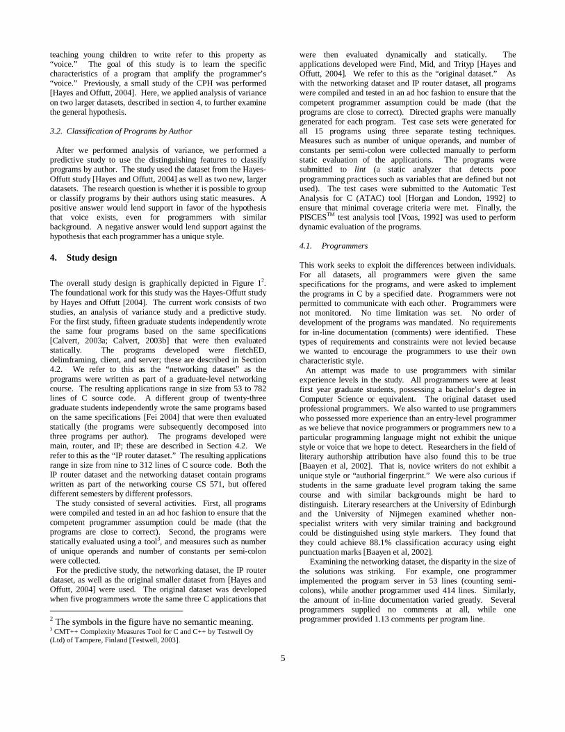
The overall study design is graphically depicted in Figure 12. The foundational work for this study was the Hayes-Offutt study by Hayes and Offutt [2004]. The current work consists of two studies, an analysis of variance study and a predictive study. For the first study, fifteen graduate students independently wrote the same four programs based on the same specifications [Calvert, 2003a; Calvert, 2003b] that were then evaluated statically. The programs developed were fletchED, delimframing, client, and server; these are described in Section 4.2. We refer to this as the “networking dataset” as the programs were written as part of a graduate-level networking course. The resulting applications range in size from 53 to 782 lines of C source code. A different group of twenty-three graduate students independently wrote the same programs based on the same specifications [Fei 2004] that were then evaluated statically (the programs were subsequently decomposed into three programs per author). The programs developed were main, router, and IP; these are described in Section 4.2. We refer to this as the “IP router dataset.” The resulting applications range in size from nine to 312 lines of C source code. Both the IP router dataset and the networking dataset contain programs written as part of the networking course CS 571, but offered different semesters by different professors. The study consisted of several activities. First, all programs were compiled and tested in an ad hoc fashion to ensure that the competent programmer assumption could be made (that the programs are close to correct). Second, the programs were statically evaluated using a tool3, and measures such as number of unique operands and number of constants per semi-colon were collected. For the predictive study, the networking dataset, the IP router dataset, as well as the original smaller dataset from [Hayes and Offutt, 2004] were used. The original dataset was developed when five programmers wrote the same three C applications that

2 The symbols in the figure have no semantic meaning.3 CMT++ Complexity Measures Tool for C and C++ by Testwell Oy (Ltd) of Tampere, Finland [Testwell, 2003].

were then evaluated dynamically and statically. The applications developed were Find, Mid, and Trityp [Hayes and Offutt, 2004]. We refer to this as the “original dataset.” As with the networking dataset and IP router dataset, all programs were compiled and tested in an ad hoc fashion to ensure that the competent programmer assumption could be made (that the programs are close to correct). Directed graphs were manually generated for each program. Test case sets were generated for all 15 programs using three separate testing techniques. Measures such as number of unique operands, and number of constants per semi-colon were collected manually to perform static evaluation of the applications. The programs were submitted to lint (a static analyzer that detects poor programming practices such as variables that are defined but not used). The test cases were submitted to the Automatic Test Analysis for C (ATAC) tool [Horgan and London, 1992] to ensure that minimal coverage criteria were met. Finally, the PISCESTM test analysis tool [Voas, 1992] was used to perform dynamic evaluation of the programs.

4.1. Programmers

This work seeks to exploit the differences between individuals. For all datasets, all programmers were given the same specifications for the programs, and were asked to implement the programs in C by a specified date. Programmers were not permitted to communicate with each other. Programmers were not monitored. No time limitation was set. No order of development of the programs was mandated. No requirements for in-line documentation (comments) were identified. These types of requirements and constraints were not levied because we wanted to encourage the programmers to use their own characteristic style. An attempt was made to use programmers with similar experience levels in the study. All programmers were at least first year graduate students, possessing a bachelor’s degree in Computer Science or equivalent. The original dataset used professional programmers. We also wanted to use programmers who possessed more experience than an entry-level programmer as we believe that novice programmers or programmers new to a particular programming language might not exhibit the unique style or voice that we hope to detect. Researchers in the field of literary authorship attribution have also found this to be true [Baayen et al, 2002]. That is, novice writers do not exhibit a unique style or “authorial fingerprint.” We were also curious if students in the same graduate level program taking the same course and with similar backgrounds might be hard to distinguish. Literary researchers at the University of Edinburgh and the University of Nijmegen examined whether non-specialist writers with very similar training and background could be distinguished using style markers. They found that they could achieve 88.1% classification accuracy using eight punctuation marks [Baayen et al, 2002]. Examining the networking dataset, the disparity in the size of the solutions was striking. For example, one programmer implemented the program server in 53 lines (counting semi-colons), while another programmer used 414 lines. Similarly, the amount of in-line documentation varied greatly. Several programmers supplied no comments at all, while one programmer provided 1.13 comments per program line.

6

Fig. 1. Overall Study Design.

4.2. Programs

For the networking dataset, a total of four programs were developed by each graduate student. Two programs were developed as part of a networking assignment on protocol layers: fletchED and delimframing. The specifications were developed by Dr. Ken Calvert of the University of Kentucky for a graduate-level Computer Science course [Calvert, 2003a]. The fletchED program implements two functions/methods as part of an error detection protocol. One method performs receiver processing and one performs sender processing. For example, the sender processing function adds a framing header to a given frame. Both functions perform error detection using the Fletcher Checksum protocol, hence the program name [Fletcher, 1982]. The delimframing program implements a framing protocol for stream channels. Two programs were developed as part of a networking assignment on challenge-response protocols and how they are used for authentication: client and server. The client program the client contacts the server and informs it of the identity (e.g., user name) to be authenticated. The server responds by sending a random “challenge” string back to the client. The client computes the MD5 hash of the bit string formed by concatenating the secret (associated with the specified user) with the challenge; it sends the result back to the server. The server (which also knows the secret associated with

the given user name) performs the same computation and compares its own result to the one received from the client. If they are equal, the server concludes that the client does indeed know the secret; otherwise the authentication fails [Calvert, 2003b]. For the IP router dataset, graduate students were given an assignment to build an IP router [Fei 2004], but were given no mandate on how to structure their implementation (as opposed to the networking dataset). Hence, some students developed one module (main.c) while other students developed three modules (main.c, router.c, and ip.c). To ensure proper comparison of the modules, we manually decomposed main.c into the three pieces (main.c, router.c, and ip.c) for students who had used only one module in their solution. There is a possibility that our decomposition may not have accurately encapsulated all the router functionality into router.c and all the ip functionality into ip.c. There is also a possibility that we did not decompose into modules the way that the student would have. However, the code that ended up in the decomposed modules was the original code written by the student, we merely broke it into pieces. For the original dataset, the three programs were Find, Mid, and Trityp. The specifications for these programs were derived from the in-line comments in implementations developed by Offutt [1992]. Figure 2 presents the specifications exactly as they were provided to the programmers.

Program 1 Program 2 Program 3

Author 1

Author 2

Author 3

Author 4

Author 5

Author 1

Author 2

Author 3

Author 4

Author 5

Author 1

Author 2

Author 3

Author 4

Author 5

Original dataset

Hayes-Offutt Study

• Identified 5 factors of interest• Provided support for CPH• Reported in [Hayes, Offutt, 2004]

CPH Evaluation(ANOVA)

• Analysis of variance• Identifies 3 features of interest• Provides support for CPH

Current work

Program Classification (PCA & LDA)

• Principal component analysis

• Linear discriminant analysis

• Classification

Dynamic andStaticmeasures

Static measures

Program 1

Author 1

.

.

.

Author 15

Networking dataset

Program 4

Author 1

.

.

.

Author 15

……..

Program 1

Author 1

.

.

.

Author 23

IP router dataset

Program 3

Author 1

.

.

.

Author 23

……..

7

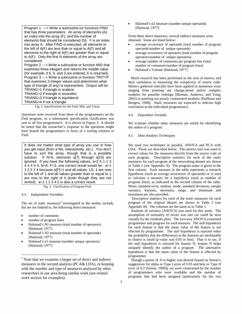
Program 1 ---> Write a subroutine (or function) FIND that has three parameters: An array of elements (A); an index into the array (F); and the number of elements that should be considered (N). F is an index into array A. After FIND is executed, all elements to the left of A(F) are less than or equal to A(F) and all elements to the right of A(F) are greater than or equal to A(F). Only the first N elements of the array are considered.Program 2 ---> Write a subroutine or function MID that examines three integers and returns the middle value (for example, if 6, 9, and 3 are entered, 6 is returned).Program 3 ---> Write a subroutine or function TRITYP that examines 3 integer values and determines what type of triangle (if any) is represented. Output will be:TRIANG=1 if triangle is scaleneTRIANG=2 if triangle is isoscelesTRIANG=3 if triangle is equilateralTRIANG=4 if not a triangle

Fig. 2. Specifications for the Find, Mid, and Trityp.

Questions were received from three of the programmers on the Find program, so a subsequent specification clarification was sent to all five programmers. It is shown in Figure 3. It should be noted that the researcher’s response to the questions might have biased the programmers in favor of a sorting solution to Find.

It does not matter what type of array you use or how you get input (from a file, interactively, etc.). You don’t have to sort the array, though that is a possible solution. If N=6, elements a[7] through a[10] are ignored. If you have the following values, a=2 5 1 1 3 4 4 4 4 4, N=6, F=3, one correct result would be: a=1 1 2 5 3 4 because a[F]=1 and all values .LE. 1 are now to the left of 1 and all values greater than or equal to 1 are now to the right of it (even though they are not sorted). a=1 1 2 3 4 5 is also a correct result.

Fig. 3. Clarification of Program Find.

4.3. Independent Variables

The set of static measures4 investigated in the studies include, but are not limited to, the following direct measures:

number of comments number of program lines Halstead’s N1 measure (total number of operators)

[Halstead, 1977] Halstead’s N2 measure (total number of operands)

[Halstead, 1977] Halstead’s n1 measure (number unique operators)

[Halstead, 1977]

4 Note that we examine a larger set of direct and indirect measures in the second analysis (PCA& LDA), in keeping with the number and type of measures analyzed by other researchers in our area doing similar work (see related work section for examples).

Halstead’s n2 measure (number unique operands) [Halstead, 1977]

From these direct measures, several indirect measures were obtained. Some are listed below: average occurrence of operands (total number of program

operands/number of unique operands) average occurrence of operators (total number of program

operators/number of unique operators) average number of comments per program line (total

number of comments/number of program lines) Halstead’s Volume [Halstead, 1977]

Much research has been performed in the area of metrics and their usefulness in measuring the complexity of source code. Metrics gathered statically have been applied in numerous ways ranging from pointing out change-prone and/or complex modules for possible redesign [Bieman, Andrews, and Yang, 2003] to pointing out poorly commented modules [Huffman and Burgess, 1988]. Static measures are expected to indicate high correlation to the individual programmers.

4.4. Dependent Variable

We evaluate whether static measures are useful for identifying the author of a program.

4.5. Data Analysis Techniques

We used two techniques in parallel, ANOVA and PCA with LDA. These are described below. The metrics tool was used to extract values for the measures directly from the source code of each program. Descriptive statistics for each of the static measures for each program of the networking dataset are shown in Table 1 (see Appendix A). The program name is given in the first column. Each measure in the table represents a research hypothesis (such as average occurrence of operands) or is used to calculate a measure for a hypothesis (such as number of program lines), as indicated in the second column of the table. Mean, standard error, median, mode, standard deviation, sample variance, kurtosis, skewness, range, and minimum and maximum are also provided. Descriptive statistics for each of the static measures for each program of the original dataset are shown in Table 2 (see Appendix B). The columns are the same as in Table 1. Analysis of variance (ANOVA) was used for this study. The assumption of normality of errors was met (as could be seen visually by the residuals plot). The two-way ANOVA examined programmer and program for each measure. The null hypothesis for each feature is that the mean value of the feature is not effected by programmer. The null hypothesis is rejected when the probability that the differences in the features are attributable to chance is small (p-value was 0.05 or less). That is to say, if the null hypothesis is rejected for feature N, feature N helps uniquely identify the author of a program. The alternative hypothesis is that the mean value of the feature is effected by programmer. Though a power of .8 or higher was desired (based on Simon’s suggestions for alpha or Type I error of 0.05 and beta or Type II error of 0.2 [Simon, 1999]), we were constrained by the number of programmers who were available and the number of programs that had been assigned (particularly for the two

8

graduate student datasets) [Power, 1999]. There is some support in the literature for studies of power of 0.4 or higher, though, particularly that involve “psychology” or social sciences [Granaas, 1999]. In fact, Granaas [1999] pointed out that the power level for published studies in psychology is around .4 (meaning a Type II error of 0.6). It could be argued that our current work is examining issues related to the psychology of programming. Therefore, our power levels may be sufficient. With alpha = 0.05, the power of the original dataset work was 0.5766 (Type II error of 0.42), the power of the networking dataset work was 0.6266 (Type II error of 0.37), and the power of the IP router dataset work was 0.4305 (Type II error of 0.57). As multi-collinearity is a known challenge when working with strongly correlated dataset variables, we chose to apply the principal component analysis technique for the second study. PCA helps to reduce the dimensions of the metric space and obtain a smaller number of orthogonal component metrics [Dillon and Goldstein, 1984]. The eigenvalue, or loading, indicates the amount of variability accounted for in the original metrics. The decision of how many components to extract is based on the cumulative proportion of eigenvalues of the principal components [Hanebutte et al, 2003]. We used the scree plot to determine the planes to retain (i.e, we kept planes with associated eigenvalues before the bend or break in the scree plot). We then applied factor analysis to these results using the varimax rotation. Basically, we examined the variables with high loadings to “label” the dimension being captured by the PC. Some dimensions were easier to explain than others. We then applied linear discriminant analysis (LDA) on the component metrics obtained from the PCA. Discriminant analysis develops a discriminant function to place each observation into one of a set of mutually exclusive classes, where prior knowledge of the classes exists [Dillon and Goldstein, 1984]. To develop the classification criterion, we used a linear method that fits a multivariate normal density to each group, with a pooled estimate of covariance [The MathWorks, Inc., 2002]. 4.6. Predictive model evaluation

To measure the accuracy of our predictive model, we carried out leave-one-out cross-validation. We used linear discriminant prediction of the authorship of a held-out program on the basis of a training set of programs with known authorship. For the networking dataset, we trained with three programs, and used the fourth program for prediction. For the original dataset, we trained on two of the three programs, and used the third program for prediction. We used jackknifing and repeated this process for all combinations of programs (e.g., trained with program 1 and 2, then trained with program 2 and 3, then trained with program 1 and 3). The discriminability of an author is the proportion of correctly attributed texts. The overall discrimination score is the average of the individual author discriminability scores [Baayen et al, 2002]. We refer to this as classification accuracy.

5. Analysis of Data

The studies had some limitations and constraints that must be kept in mind when examining the results. Threats to validity are discussed in Section 5.1. For the analysis of variance study, data was analyzed to look for an effect based on programmer (or

author), addressed in Section 5.2. The predictive study is addressed in Section 5.3. The overall hypothesis results are discussed in Section 5.4.

5.1. Threats to validity

The results from this study are subject to a number of limitations. In particular, internal and external validity are of concern. A study can be said to be internally valid if it shows a causal relationship between the independent and dependent variables. A number of influences can impact internal validity. For example, in the original dataset, we may have influenced the programmers’ solution to the Find program when we answered their questions on the specification. However, this could have only served to prompt the programmers to use a similar solution, resulting in similar programs. So any bias would have been in favor of the null hypothesis. In order to minimize selection threats to internal validity, we assigned each programmer the same programs (for all datasets). Also, we did not mandate the order in which the programs were developed. Another threat to internal validity is that of programmers biasing each other. Specifically, on the original dataset, two of the programmers work in the same location and may have discussed the programs, causing their solutions to be similar (though no correlation was found between the programs of these two authors). Similarly, it is possible that the graduate students may have discussed the networking programs. We asked each programmer to work in isolation to minimize this threat [Hayes and Offutt, 2004] and graduate students were warned not to work together. Experimental mortality threats to internal validity were not applicable, as all programmers completed the assigned programs [Hayes and Offutt, 2004]. Design contamination threats to internal validity were not applicable, as there was not a separate control and experimental group [Hayes and Offutt, 2004]. There is a possibility of an instrumentation threat to internal validity (see section 4.4) due to switching to a commercial tool for the networking dataset. External validity is possessed by a study if the causal relationship can be generalized to other groups, environments, etc. There were several threats to external validity in our study. First, a small number of programmers were used in the original dataset (five). Each programmer wrote a small number of programs (three in the original dataset, four in the networking dataset, three in the IP router dataset). The networking and IP router datasets had more data points. Declining results as datasets get larger may indicate that these techniques can only distinguish among small numbers of programmers. Also, the original dataset programs were very small and were not very complicated to write. It is not certain that the results seen here would be observed for larger, more complex applications, though the networking and IP router datasets did allow us to examine programs that were larger and more complex than the original dataset. Also, two of the three datasets were from the networking application domain. Additional datasets from different application domains (such as medical applications, avionic software applications, etc.) should be evaluated to ensure that the results observed can be generalized across multiple application domains. Also, there is a potential bias since all the original dataset programmers are from the Washington metropolitan area and most of them (four of the five) work for defense contractors. Also, all the graduate

9

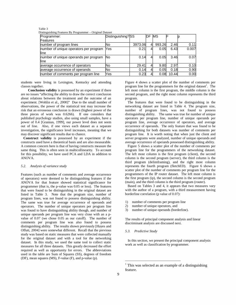
Table 3 Distinguishing Features By Programmer – Original Dataset

Programmer:Features

Distinguishing? SS DF MS F p

number of program lines No 3973.06 4 993.26 2.46 0.11number of unique operators per program line

Yes 0.21 4 0.05 6.43 0.007

number of unique operands per program line

No 0.14 4 0.05 3.46 0.07

average occurrence of operators No 29.41 4 9.80 2.97 0.10average occurrence of operands No 0.14 4 0.05 0.18 0.90number of comments per program line Yes 0.23 4 0.08 10.44 0.00

students were living in Lexington, Kentucky and attending classes together. Conclusion validity is possessed by an experiment if there are no issues “affecting the ability to draw the correct conclusion about relations between the treatment and the outcome of an experiment. [Wohlin et al., 2000]” Due to the small number of observations, the power of the statistical test may increase the risk that an erroneous conclusion is drawn (highest power of the three pieces of work was 0.6266). If one considers that published psychology studies, also using small samples, have a power of 0.4 [Grannas, 1999], our power level does not seem out of line. Also, if one views each dataset as a separate investigation, the significance level increases, meaning that we may discover significant results due to chance. Construct validity is possessed by an experiment if the constructs used have a theoretical basis and are also measurable. A common concern here is that of having constructs measure the same thing. This is often seen in multicollinearity. To account for this possibility, we have used PCA and LDA in addition to ANOVA.

5.2. Analysis of variance study

Features (such as number of comments and average occurrence of operators) were deemed to be distinguishing features if the ANOVA for that feature showed statistical significance for programmer (that is, the p-value was 0.05 or less). The features that were found to be distinguishing in the original dataset are listed in Table 3. Note that the program size, number of program lines, was not found to possess distinguishing ability. The same was true for average occurrence of operands and operators. The number of unique operators per program line was found to have distinguishing ability though, and number of unique operands per program line was very close with an a p-value of 0.07 (we chose 0.05 as our cutoff). The number of comments per program line was also found to possess distinguishing ability. The results shown previously [Hayes and Offutt, 2004] were somewhat different. Recall that the previous study was based on static measures that were collected manually for the original dataset and with a tool for the networking dataset. In this study, we used the same tool to collect static measures for all three datasets. This greatly decreased the effort required as well as opportunity for errors. The abbreviations used in the table are Sum of Squares (SS), degrees of freedom (DF), mean squares (MS), F-value (F), and p-value (p).

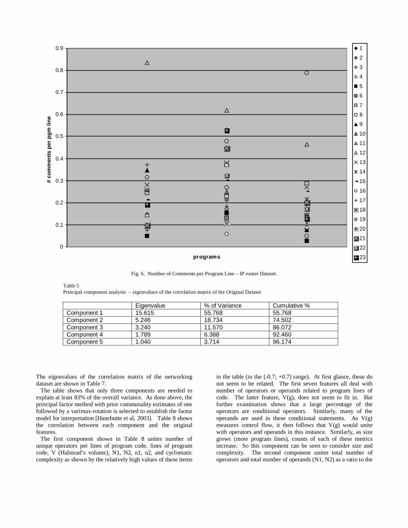
Figure 4 shows a scatter plot of the number of comments per program line for the programmers for the original dataset1. The left most column is the first program, the middle column is the second program, and the right most column represents the third program. The features that were found to be distinguishing in the networking dataset are listed in Table 4. The program size, number of program lines, was not found to possess distinguishing ability. The same was true for number of unique operators per program line, number of unique operands per program line, average occurrence of operators, and average occurrence of operands. The only feature that was found to be distinguishing for both datasets was number of comments per program line. It is worth noting that when just the client and server programs were analyzed, number of unique operands and average occurrence of operands possessed distinguishing ability. Figure 5 shows a scatter plot of the number of comments per program line for the programmers of the networking dataset. The left most column is the first program (client), the second column is the second program (server), the third column is the third program (delimframing), and the right most column represents the fourth program (fletchED). Figure 6 shows a scatter plot of the number of comments per program line for the programmers of the IP router dataset. The left most column is the first program (ip), the second column is the second program (main), and the third column is the third program (router). Based on Tables 3 and 4, it appears that two measures vary with the author of a program, with a third measurement having borderline correlation (p value of 0.07):

1) number of comments per program line2) number of unique operators, and3) number of unique operands (borderline).

The results of principal component analysis and linear discriminant analysis are discussed next.

5.3. Predictive Study

In this section, we present the principal component analysis work as well as classification by programmer.

1 This was selected as an example of a distinguishing feature.

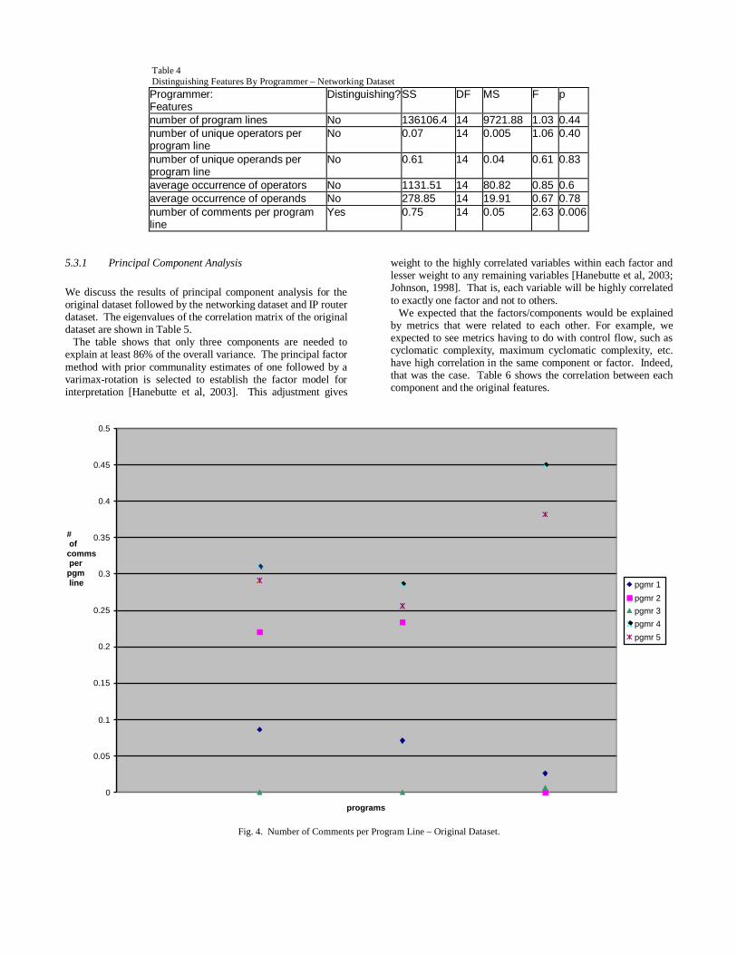
Table 4Distinguishing Features By Programmer – Networking Dataset

Programmer:Features

Distinguishing?SS DF MS F p

number of program lines No 136106.4 14 9721.88 1.03 0.44number of unique operators per program line

No 0.07 14 0.005 1.06 0.40

number of unique operands per program line

No 0.61 14 0.04 0.61 0.83

average occurrence of operators No 1131.51 14 80.82 0.85 0.6average occurrence of operands No 278.85 14 19.91 0.67 0.78number of comments per program line

Yes 0.75 14 0.05 2.63 0.006

5.3.1 Principal Component Analysis

We discuss the results of principal component analysis for the original dataset followed by the networking dataset and IP router dataset. The eigenvalues of the correlation matrix of the original dataset are shown in Table 5. The table shows that only three components are needed to explain at least 86% of the overall variance. The principal factor method with prior communality estimates of one followed by a varimax-rotation is selected to establish the factor model for interpretation [Hanebutte et al, 2003]. This adjustment gives

weight to the highly correlated variables within each factor and lesser weight to any remaining variables [Hanebutte et al, 2003; Johnson, 1998]. That is, each variable will be highly correlated to exactly one factor and not to others. We expected that the factors/components would be explained by metrics that were related to each other. For example, we expected to see metrics having to do with control flow, such as cyclomatic complexity, maximum cyclomatic complexity, etc. have high correlation in the same component or factor. Indeed, that was the case. Table 6 shows the correlation between each component and the original features.

0

0.05

0.1

0.15

0.2

0.25

0.3

0.35

0.4

0.45

0.5

programs

# ofcomms per pgm line pgmr 1

pgmr 2

pgmr 3

pgmr 4

pgmr 5

Fig. 4. Number of Comments per Program Line – Original Dataset.

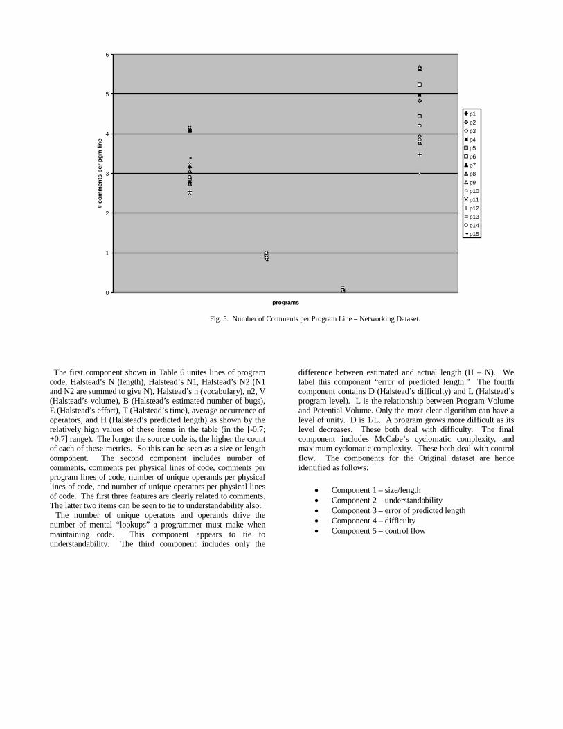
Fig. 5. Number of Comments per Program Line – Networking Dataset.

The first component shown in Table 6 unites lines of program code, Halstead’s N (length), Halstead’s N1, Halstead’s N2 (N1 and N2 are summed to give N), Halstead’s n (vocabulary), n2, V (Halstead’s volume), B (Halstead’s estimated number of bugs), E (Halstead’s effort), T (Halstead’s time), average occurrence of operators, and H (Halstead’s predicted length) as shown by the relatively high values of these items in the table (in the [-0.7; +0.7] range). The longer the source code is, the higher the count of each of these metrics. So this can be seen as a size or length component. The second component includes number of comments, comments per physical lines of code, comments per program lines of code, number of unique operands per physical lines of code, and number of unique operators per physical lines of code. The first three features are clearly related to comments. The latter two items can be seen to tie to understandability also. The number of unique operators and operands drive the number of mental “lookups” a programmer must make when maintaining code. This component appears to tie to understandability. The third component includes only the

difference between estimated and actual length (H – N). We label this component “error of predicted length.” The fourth component contains D (Halstead’s difficulty) and L (Halstead’s program level). L is the relationship between Program Volumeand Potential Volume. Only the most clear algorithm can have a level of unity. D is 1/L. A program grows more difficult as its level decreases. These both deal with difficulty. The final component includes McCabe’s cyclomatic complexity, and maximum cyclomatic complexity. These both deal with control flow. The components for the Original dataset are hence identified as follows:

Component 1 – size/length Component 2 – understandability Component 3 – error of predicted length Component 4 – difficulty Component 5 – control flow

0

1

2

3

4

5

6

programs

# c

om

me

nts

pe

r p

gm

lin

e

p1

p2

p3

p4

p5

p6

p7

p8

p9

p10

p11

p12

p13

p14

p15

0

0.1

0.2

0.3

0.4

0.5

0.6

0.7

0.8

0.9

programs

# co

mm

ents

per

pg

m l

ine

1

2

3

4

5

6

7

8

9

10

11

12

13

14

15

16

17

18

19

20

21

22

23

Fig. 6. Number of Comments per Program Line – IP router Dataset.

Table 5Principal component analysis – eigenvalues of the correlation matrix of the Original Dataset

Eigenvalue % of Variance Cumulative %Component 1 15.615 55.768 55.768Component 2 5.246 18.734 74.502Component 3 3.240 11.570 86.072Component 4 1.789 6.388 92.460Component 5 1.040 3.714 96.174

The eigenvalues of the correlation matrix of the networking dataset are shown in Table 7. The table shows that only three components are needed to explain at least 83% of the overall variance. As done above, the principal factor method with prior communality estimates of one followed by a varimax-rotation is selected to establish the factor model for interpretation [Hanebutte et al, 2003]. Table 8 shows the correlation between each component and the original features. The first component shown in Table 8 unites number of unique operators per lines of program code, lines of program code, V (Halstead’s volume), N1, N2, n1, n2, and cyclomatic complexity as shown by the relatively high values of these items

in the table (in the [-0.7; +0.7] range). At first glance, these do not seem to be related. The first seven features all deal with number of operators or operands related to program lines of code. The latter feature, V(g), does not seem to fit in. But further examination shows that a large percentage of the operators are conditional operators. Similarly, many of the operands are used in these conditional statements. As V(g) measures control flow, it then follows that V(g) would unite with operators and operands in this instance. Similarly, as size grows (more program lines), counts of each of these metrics increase. So this component can be seen to consider size and complexity. The second component unites total number of operators and total number of operands (N1, N2) as a ratio to the

13

number of unique operators and operands, as well as these same features divided by program lines. This appears to capture adegree of variance dealing with the number of mental recollections a programmer must make when maintaining a program. We refer to this as maintenance effort. The third component includes only unique operands per program line. This does not appear to capture an intuitive source of variance. The final component captures comments per program line. As with the original dataset, we believe this component ties to

understandability. The components for the Networking dataset are hence identified as follows:

Component 1 – size/complexityComponent 2 – maintenance effortComponent 3 – unknownComponent 4 – understandability

Table 6Rotated components of original dataset – five components selected

.318 .229 .179 .186 .864

.096 -.309 .231 -.045 .886

.687 .682 .152 .058 -.031

.806 .488 .236 .021 .111

.488 .638 .043 .109 -.319

.462 .856 -.040 .074 -.093

.966 .168 .117 .122 .096

.947 .180 .167 .114 .147

.973 .154 .065 .128 .042

.952 .170 -.169 .161 .072

.694 .010 -.163 .675 .075

.961 .206 -.159 -.003 .066

.974 .166 .068 .106 .078

.934 .106 .120 .304 .060

.647 -.061 .195 .719 .053

.950 .111 .104 .224 .023

-.548 -.009 -.227 -.757 -.123

.950 .111 .104 .224 .023

.318 -.138 .695 .577 .058

.822 .231 .387 -.213 .220

.959 .168 -.167 .127 .063

.032 .000 .957 .039 .227

.162 .923 -.143 -.034 -.024

.101 .954 -.189 -.008 -.059

.111 -.847 -.500 -.037 -.056

.078 -.630 -.684 .011 -.227

-.311 -.762 -.295 .431 -.107

-.396 -.628 -.351 .491 -.219

V(G)

Max v(G)

LOCphy

LOCpro

LOCbl

LOCcomN

N1

N2

n

n1

n2

V

B

D

E

LT

Avg occ. opds

Avg occ. ops

HH-NComm/locphy

n2/locphy

n2/locpro

n1/locphy

n1/locpro

1 2 3 4 5

Component

Comm/locpro

The eigenvalues of the correlation matrix of the IP router dataset are shown in Table 9. The table shows that only three components are needed to explain at least 79% of the overall variance. As done above, the principal factor method with prior communality estimates of one followed by a varimax-rotation is selected to establish the factor model for interpretation [Hanebutte et al, 2003]. Table 10 shows the correlation between each component and the original features. The first component shown in Table 10 unites average occurrence of operands, average occurrence of operators, number of unique operators (n1) per physical line, and number of unique operators (n1) per program line as shown by the relatively high values of these items in the table (in the [-0.7; +0.7] range). Just as with Component 2 of the networking dataset, this appears to capture a degree of variance dealing with the number of mental recollections a programmer must make

when maintaining a program. We refer to this as maintenance effort. The second component captures comments per program line and comments per physical line. As with the original dataset and the networking dataset, we believe this component ties to understandability. The third component includes only unique operands (n2) per program line. This does not appear to capture an intuitive source of variance. However, it is identical to the “unknown” Component 3 of the networking dataset. It appears that number of unique operands per program line is capturing a recurring source of variance. The components are hence identified as follows:

Component 1 – maintenance effortComponent 2 – understandabilityComponent 3 – unknown

Table 7Principal component analysis – eigenvalues of the correlation matrix of the Networking Dataset

Eigenvalue % of Variance Cumulative %Component 1 7.417 46.357 46.357Component 2 3.993 24.955 71.312Component 3 1.948 12.175 83.487Component 4 1.466 9.162 92.649

Table 8Rotated components of networking dataset – four components selected

-.892 -.021 .208 .133

-.358 -.043 .887 .104

.962 -.058 -.026 .047

.585 .007 -.007 .775

.949 .047 .225 .087

.635 -.033 .695 -.009

.768 .632 .039 .053

.739 .661 .059 .069

.815 -.104 .056 .081

.719 -.051 .668 .029

.532 .827 -.043 -.002

-.003 .877 -.452 -.021

-.128 .017 .090 .968

.881 .122 -.097 .084

-.145 .980 .058 -.005

-.165 .975 .068 .024

n1/prog line

n2/prog line

LOCpro

LOCcom

V

B(x100)

N1

N2

n1

n2

N1/n1

N2/n2

com/prog line

V(g)

N1/prog line

N2/prog line

1 2 3 4

Component

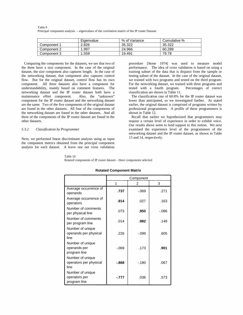
Table 9Principal component analysis – eigenvalues of the correlation matrix of the IP router Dataset

Eigenvalue % of Variance Cumulative %Component 1 2.826 35.322 35.322Component 2 1.997 24.966 60.289Component 3 1.559 19.491 79.78

Comparing the components for the datasets, we see that two of the three have a size component. In the case of the original dataset, the size component also captures length. In the case of the networking dataset, that component also captures control flow. But for the original dataset, control flow has its own component. All three datasets also have a component for understandability, mainly based on comment features. The networking dataset and the IP router dataset both have a maintenance effort component. Also, the “unknown” component for the IP router dataset and the networking dataset are the same. Two of the five components of the original dataset are found in the other datasets. All four of the components of the networking dataset are found in the other datasets. And all three of the components of the IP router dataset are found in the other datasets.

5.3.2 Classification by Programmer

Next, we performed linear discriminant analysis using as input the component metrics obtained from the principal component analysis for each dataset. A leave one out cross validation

procedure [Stone 1974] was used to measure model performance. The idea of cross validation is based on using a training subset of the data that is disjunct from the sample or testing subset of the dataset. In the case of the original dataset, we trained with two programs and tested on the third program. For the networking dataset, we trained with three programs and tested with a fourth program. Percentages of correct classification are shown in Table 11. The classification rate of 60.8% for the IP router dataset was lower than anticipated, so we investigated further. As stated earlier, the original dataset is comprised of programs written by professional programmers. A profile of these programmers is shown in Table 12. Recall that earlier we hypothesized that programmers may require a certain level of experience in order to exhibit voice. Our results above seem to lend support to this notion. We next examined the experience level of the programmers of the networking dataset and the IP router dataset, as shown in Table 13 and 14, respectively.

Table 10Rotated components of IP router dataset – three components selected

Rotated Component Matrix

.737 -.069 .271

.914 .027 .163

.073 .950 -.086

.014 .982 .149

.226 -.099 .605

-.069 .173 .901

-.868 -.180 .067

-.777 .036 .573

Average occurrence ofoperands

Average occurrence ofoperators

Number of commentsper physical line

Number of commentsper program line

Number of uniqueoperands per physicalline

Number of uniqueoperands perprogram line

Number of uniqueoperators per physicalline

Number of uniqueoperators perprogram line

1 2 3

Component

Table 11Percentages of correct classifications (cross validation)

Dataset % correct classificationOriginal dataset 100%

Networking dataset 93.33%IP router dataset 60.8%

Table 12Profile of original dataset programmers

Programmer Employer Highest Degree Work Experience

1 IT Company 1 M.S. in SWE in 2 months

Programmer, Analyst

2 IT Company 2 M.S. in CS Programmer, Analyst

3 IT Company 2 M.S. in CS Analyst, Programmer

4 IT Company 3 M.S. in CS Programmer, Analyst

5 University Ph.D. CS Asst. Professor, Programmer

To see whether or not we could correctly classify experienced C and networking programmers, we selected a subset of the programmers of the IP router dataset for analysis. The criteria we used for selecting the first subset of programmers was that they must be very experienced in C and have strong work experience OR they must possess strong networking experience. Based on this, we selected Programmers 2, 3, 6, 13 and 20 (2, 3, and 20 for C and work experience, ands 6 and 13 for networking experience). We refer to this as the (C^Work)vNetworks subset.

Next, we eased our criteria and added any students who had taken an undergraduate course in networking, regardless of their C or work experience. This second subset included the first subset plus Programmers 10, 11, 16, and 21. We refer to this asthe (C^Work)v (Networks)v(undergradcourse) subset. The results are shown below in Table 15. This appears to lend support for the notion of a certain level of experience being required before a programmer exhibits voice.

17

Table 13Profile of networking dataset programmers

5.4. Hypothesis results

The general hypothesis for this experiment is that one or more characteristics exist for a program that can recognize the author of the program. This is important to help pursue specific rogue programmers of malicious code and source code viruses, to identify the author of non-commented source code that we are trying to maintain, and to help detect plagiarism and copyright violation of source code. Evidence has been presented in Section 5.2 to support the notion that characteristics exist to identify the author of a program. Some of the specific hypotheses were supported and some were not. The results are listed below:

1. Evidence was found to reject the null hypothesis that the static measure of number of comments per program linedoes not vary by individual programmer.

2. The null hypothesis that the static measure of average occurrence of operands does not vary by individual programmer could not be rejected.

3. The hypothesis that the static measure of average occurrence of operators is correlated with the individual programmer was not supported, however there was evidence that number of unique operators does vary by individual programmer.

Programmer Commenced Graduate Work

Prior C experience Prior networking programming experience

Work Experience

1 Fall 2001 Used C occasionally None Programmer for one year, using C++

2 Spring 2001 Programmer for two years

3 Fall 2002 No prior experience in C or C-like language

Minimal prior experience Some DB work experience with minimal networking work experience

4 Fall 2002 3 – 4 years experience None System administrator/programmer for 3 – 4 years

5 Fall 2002 ~10 months experience with C

~10 months networking programming experience in C

~10 months networking programming experience in C

6 Fall 2002 Used C in some undergrad courses

Minimal prior experience None

7 Fall 2002 ~4 years experience with C

Undergraduate project in networking programming

Taught programming languages

8 Fall 2002 Used C occasionally None None9 Fall 2002 8 years of C experience Minimal networking

programming experience

None

10 Fall 2002 Very little programming experience

Did one networking exercise in VC++ in undergrad work

None

11 N/A, was undergraduate Used C in UK courses Took networking 400 level course

Coop at Lexmark using C, some networking assignments

12 Fall 2002 Had C in undergrad courses

Built a small networking program previously

None

13 Fall 2002 Some C and C++ experience

Some networking programming experience

4 years as a programmer/system analyst

14 Fall 2002 Little programming experience in C from undergrad

Undergrad network management project

None

15 Fall 2002 Minimal C experience (from high school)

Networking experience was from undergrad class

None

18

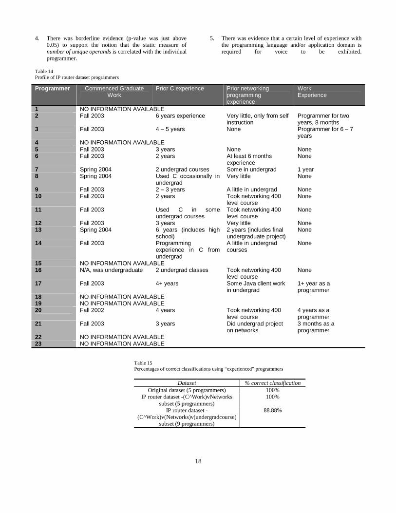
4. There was borderline evidence (p-value was just above 0.05) to support the notion that the static measure of number of unique operands is correlated with the individual programmer.

5. There was evidence that a certain level of experience with the programming language and/or application domain is required for voice to be exhibited.

Table 14Profile of IP router dataset programmers

Table 15Percentages of correct classifications using “experienced” programmers

Dataset % correct classificationOriginal dataset (5 programmers) 100%

IP router dataset -(C^Work)vNetworkssubset (5 programmers)

100%

IP router dataset -(C^Work)v(Networks)v(undergradcourse)

subset (9 programmers)

88.88%

Programmer Commenced Graduate Work

Prior C experience Prior networking programming experience

Work Experience

1 NO INFORMATION AVAILABLE2 Fall 2003 6 years experience Very little, only from self

instructionProgrammer for two years, 8 months

3 Fall 2003 4 – 5 years None Programmer for 6 – 7 years

4 NO INFORMATION AVAILABLE5 Fall 2003 3 years None None6 Fall 2003 2 years At least 6 months

experienceNone

7 Spring 2004 2 undergrad courses Some in undergrad 1 year8 Spring 2004 Used C occasionally in

undergradVery little None

9 Fall 2003 2 – 3 years A little in undergrad None10 Fall 2003 2 years Took networking 400

level courseNone

11 Fall 2003 Used C in some undergrad courses

Took networking 400 level course

None

12 Fall 2003 3 years Very little None13 Spring 2004 6 years (includes high

school)2 years (includes final undergraduate project)

None

14 Fall 2003 Programming experience in C from undergrad

A little in undergrad courses

None

15 NO INFORMATION AVAILABLE16 N/A, was undergraduate 2 undergrad classes Took networking 400

level courseNone

17 Fall 2003 4+ years Some Java client work in undergrad

1+ year as a programmer

18 NO INFORMATION AVAILABLE19 NO INFORMATION AVAILABLE20 Fall 2002 4 years Took networking 400

level course4 years as a programmer

21 Fall 2003 3 years Did undergrad project on networks

3 months as a programmer

22 NO INFORMATION AVAILABLE23 NO INFORMATION AVAILABLE

19

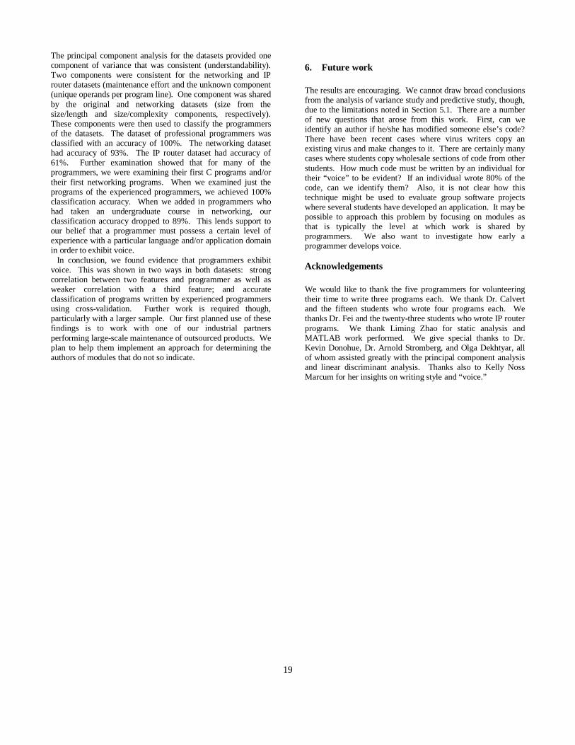
The principal component analysis for the datasets provided one component of variance that was consistent (understandability). Two components were consistent for the networking and IP router datasets (maintenance effort and the unknown component (unique operands per program line). One component was shared by the original and networking datasets (size from the size/length and size/complexity components, respectively). These components were then used to classify the programmers of the datasets. The dataset of professional programmers was classified with an accuracy of 100%. The networking dataset had accuracy of 93%. The IP router dataset had accuracy of 61%. Further examination showed that for many of the programmers, we were examining their first C programs and/or their first networking programs. When we examined just the programs of the experienced programmers, we achieved 100% classification accuracy. When we added in programmers who had taken an undergraduate course in networking, our classification accuracy dropped to 89%. This lends support to our belief that a programmer must possess a certain level of experience with a particular language and/or application domain in order to exhibit voice. In conclusion, we found evidence that programmers exhibit voice. This was shown in two ways in both datasets: strong correlation between two features and programmer as well as weaker correlation with a third feature; and accurate classification of programs written by experienced programmers using cross-validation. Further work is required though, particularly with a larger sample. Our first planned use of these findings is to work with one of our industrial partners performing large-scale maintenance of outsourced products. We plan to help them implement an approach for determining the authors of modules that do not so indicate.

6. Future work

The results are encouraging. We cannot draw broad conclusions from the analysis of variance study and predictive study, though, due to the limitations noted in Section 5.1. There are a number of new questions that arose from this work. First, can we identify an author if he/she has modified someone else’s code? There have been recent cases where virus writers copy an existing virus and make changes to it. There are certainly many cases where students copy wholesale sections of code from other students. How much code must be written by an individual for their “voice” to be evident? If an individual wrote 80% of the code, can we identify them? Also, it is not clear how this technique might be used to evaluate group software projects where several students have developed an application. It may be possible to approach this problem by focusing on modules as that is typically the level at which work is shared by programmers. We also want to investigate how early a programmer develops voice.

Acknowledgements

We would like to thank the five programmers for volunteering their time to write three programs each. We thank Dr. Calvert and the fifteen students who wrote four programs each. We thanks Dr. Fei and the twenty-three students who wrote IP router programs. We thank Liming Zhao for static analysis and MATLAB work performed. We give special thanks to Dr. Kevin Donohue, Dr. Arnold Stromberg, and Olga Dekhtyar, all of whom assisted greatly with the principal component analysis and linear discriminant analysis. Thanks also to Kelly Noss Marcum for her insights on writing style and “voice.”

20

APPENDIX A

Table 1Descriptive Statistics of Static Measures Collected for Networking Dataset

Program ResearchHypothesis

Measure Mean Std Error

Median Mode Std Dev.

Sample Variance

Kurtosis Skewness Range Min Max

delimframing For R1, R2, R3

Number of program lines

242.45 18.63 209.50 208 87.38 7635.21 1.27 1.29 332.00 136.00 468.00

delimframing For R3 Number of operators

612.05 53.00 542.50 490 248.58 61791.57 2.25 1.40 1015.00 323.00 1338.00

delimframing For R2 Number of operands

532.14 46.07 479.00 N/A 216.11 46701.46 1.67 1.29 859.00 273.00 1132.00

delimframing R4 Number of unique operands

68.05 3.27 66.00 58 15.35 235.47 2.18 1.27 66.00 46.00 112.00

delimframing R2 Average occurrence of operands

7.84 0.64 7.06 N/A 2.98 8.89 5.63 2.31 12.71 4.71 17.42

delimframing R3 Average occurrence of operators

21.18 1.65 19.53 N/A 7.76 60.25 1.03 1.20 28.59 10.77 39.35

delimframing R1 Number of comments per program line

0.29 0.06 0.19 N/A 0.26 0.07 4.31 1.93 1.10 0.03 1.13

fletchED For R1, R2, R3

Number program lines

118.55 6.73 113.00 130 31.58 997.12 -0.76 0.43 109.00 70.00 179.00

fletchED For R3 Number operators

295.36 15.42 289.00 339 72.34 5232.43 -1.06 0.35 245.00 191.00 436.00

fletchED For R2 Number operands

270.41 14.31 266.50 N/A 67.13 4505.87 -0.82 0.49 215.00 184.00 399.00

fletchED R4 Number unique operands

42.23 1.12 44.00 44 5.25 27.52 -0.09 -0.13 22.00 31.00 53.00

fletchED R2 Average occurrence operands

6.35 0.22 6.18 N/A 1.05 1.09 -1.12 0.37 3.28 4.95 8.23

fletchED R3 Average occurrence operators

11.66 0.57 11.70 N/A 2.68 7.19 -0.46 0.56 9.47 7.93 17.39

fletchED R1 Number of comments/ program line

0.25 0.05 0.17 0 0.25 0.06 3.52 1.77 1.04 0.00 1.04

client For R1, R2, R3

Number program lines

180.54 22.88 187.00 N/A 82.49 6804.77 -0.62 -0.01 269.00 59.00 328.00

client For R3 Number operators

486.00 56.28 523.00 N/A 202.91 41171.83 -1.33 -0.32 570.00 182.00 752.00

client For R2 Number operands

446.38 50.31 473.00 N/A 181.38 32899.92 -1.30 -0.42 496.00 162.00 658.00

client R4 Number uniqueoperands

119.46 10.68 109.00 N/A 38.51 1482.94 -1.20 0.22 113.00 66.00 179.00

client R2 Average occurrence operands

3.66 0.25 3.77 N/A 0.89 0.80 -0.75 -0.01 3.02 2.13 5.15

21

client R3 Average occurrence operators

17.54 1.36 20.12 N/A 4.92 24.17 -0.25 -0.78 16.26 8.27 24.54

client R1 Number comments/program line

45.77 9.33 33.00 N/A 33.65 1132.53 -0.08 0.96 106.00 5.00 111.00

server For R1, R2, R3

Number program lines

249.46 31.27 247.00 234.00 112.74 12711.10 -0.38 -0.45 361.00 53.00 414.00

server For R3 Number operators

648.92 75.79 656.00 N/A 273.25 74667.74 -0.10 -0.77 831.00 149.00 980.00

server For R2 Number operands

582.15 69.68 585.00 N/A 251.24 63119.14 -0.27 -0.66 774.00 132.00 906.00

server R4 Number unique operands

151.08 14.66 154.00 168.00 52.84 2792.24 0.59 -0.02 193.00 63.00 256.00

server R2 Average occurrence operands

3.71 0.28 3.94 N/A 1.01 1.02 1.41 0.40 3.90 2.10 6.00

server R3 Average occurrence operators

20.86 1.89 22.71 N/A 6.82 46.49 -0.35 -0.71 21.36 8.33 29.70

server R1 Number of comments/program line

52.92 9.39 42.00 42.00 33.85 1145.58 2.13 1.43 124.00 13.00 137.00

22

APPENDIX B

Table 2Descriptive Statistics of Static Measures Collected for Original Dataset

Program ResearchHypothesis

Measure Mean Std Error

Median Mode Std Dev.

Sample Variance

Kurtosis Skewness Range Min Max

find For R1, R2, R3

Number of program lines

71.80 13.10 81.00 N/A 29.30 858.70 -0.93 -0.02 75.00 35.00 110.00

find For R3 Number of unique operators per program line

0.32 0.05 0.28 N/A 0.12 0.01 -0.89 0.58 0.29 0.19 0.49

find For R2, R4 Number of unique operands per program line

0.65 0.07 0.74 N/A 0.17 0.03 -2.87 -0.60 0.36 0.44 0.80

find R2 Average occurrence of operands

4.04 0.17 4.19 N/A 0.38 0.15 0.18 -0.89 0.98 3.46 4.44

find R3 Average occurrence of operators

8.98 0.96 7.62 N/A 2.14 4.56 -1.71 0.87 4.71 7.29 12.00

find R1 Number of comments per program line

0.18 0.06 0.22 N/A 0.13 0.02 -1.89 -0.58 0.31 0.00 0.31

mid For R1, R2, R3

Number of program lines

39.00 6.98 35.00 N/A 15.60 243.50 1.36 1.27 39.00 25.00 64.00

mid For R3 Number of unique operators per program line

0.40 0.08 0.34 N/A 0.18 0.03 4.33 2.02 0.45 0.27 0.72

mid For R2, R4 Number of unique operands per program line

0.61 0.08 0.57 N/A 0.18 0.03 -2.37 0.40 0.40 0.44 0.84

mid R2 Average occurrence of operands

3.45 0.21 3.52 N/A 0.47 0.22 -0.48 0.08 1.21 2.86 4.07

mid R3 Average occurrence of operators

6.19 0.70 5.80 N/A 1.57 2.47 1.89 0.88 4.31 4.33 8.65

mid R1 Number of comments per program line

0.17 0.06 0.23 N/A 0.13 0.02 -2.20 -0.69 0.29 0.00 0.29

trityp For R1, R2, R3

Number of program lines

50.80 6.45 49.00 N/A 14.41 207.70 -2.65 0.22 32.00 36.00 68.00

trityp For R3 Number of unique operators per program line

0.39 0.07 0.37 N/A 0.15 0.02 2.32 1.45 0.38 0.25 0.64

trityp For R2, R4 Number of unique operands per program line

0.59 0.04 0.57 N/A 0.10 0.01 -1.13 -0.29 0.23 0.46 0.69

trityp R2 Average occurrence of operands

3.74 0.28 3.69 N/A 0.63 0.39 -1.89 0.36 1.45 3.12 4.57

trityp R3 Average occurrence of operators

7.03 0.72 7.00 N/A 1.61 2.59 0.26 0.53 4.25 5.13 9.38

trityp R1 Number of comments per program line

0.17 0.10 0.03 0.00 0.22 0.05 -3.03 0.65 0.45 0.00 0.45

23

References

Baayen, H., van Halteren, Neijt, A., and Tweedie, F. 2002. An experiment in authorship attribution. In Proceedings of the 6s Journies Internationales dAnalyse de Donnies Textuelles (JADT), Malo, France, 13-15 March.

Bieman, J., Andrews, A., and Yang, H. 2003. Understanding change-proneness in OO software through visualization. The 11th IEEE International Workshop on Program Comprehension (IWPC'03), Portland, Oregon, 10 – 11 May.

Briand, L., Basili, V. and Hetmanski, C. 1993. Developing Interpretable Models with Optimized Set Reduction for Identifying High-Risk Software Components. IEEE Trans. Software Eng. 19(11): 1028-1044.

Briand, L., Melo, W., and Wust, J. 2002. Assessing the applicability of fault-proneness models across object-oriented software projects. IEEE Transactions on Software Engineering 28(7):706 – 720.

Brooks, F. 1987. No silver bullet: Essence and accidents of software engineering. IEEE Computer 20(4):10-19.

Calvert, Ken. 2003a. Programming Assignment 0: Protocol Layers, Version 1.2. CS 571 Computer Networks, University of Kentucky, Spring 2003.

Calvert, Ken. 2003b. Programming Assignment 1: Challenge-Response Authentication. CS 571 Computer Networks, University of Kentucky, Spring 2003.

Collberg, Christian, and Thomborson, Clark. 2000. Watermarking, tamper-proofing, and obfuscation - Tools for software protection. University of Arizona Computer Science Technical Report number 2000-03, February 10, 2000, pp. 5-7.

Corney, M., de Vel, O., Anderson, A., and Mohay, G. 2002. Gender-preferential text mining of e-mail discourse. In Proceedings of the Annual Computer Security Applications Conference.

DeMillo, Richard A., Lipton, Richard J., and Sayward, Frederick G. 1978. Hints on test data selection: Help for the practicing programmer, IEEE Computer 11(4): 34-41.

de Vel, O., Anderson, A., Corney, M., and Mohay G. 2001. Mining e-mail content for author identification forensics. SIGMOD Record30(4):55 – 64.

Dillon, W., and Goldstein, M. 1984. Multivariate Analysis: Methods and Applications, John Wiley and Sons, New York, New York.

Fei, Z. 2004. Project 1: IP Router Implementation. CS 571 Computer Networks, University of Kentucky, Spring 2004.

Finkel, R., Zaslavsky, A., Monostori, K., and Schmidt, H. 2002. In Proceedings of the Twenty-Fifth Australasian Computer Science Conference (ACSC2002).

Fletcher, J.G. 1982. An arithmetic checksum for serial transmission. IEEE Transactions on Communications (COM-30):1.

Granaas, M. 1999. Re: Type I and Type II error. Educational Statistics Discussion List (EDSTAT-L). [Online]. Available E-mail: edstat-l@jse.stat.ncsu.edu January 7, 1999.

Gray, A. R., Sallis, P. J., and MacDonell, S. G. 1998. IDENTIFIED (Integrated Dictionary-based Extraction of Non-language-dependent Token Information for Forensic Identification, Examination, and Discrimination): A dictionary-based system for extracting source code

metrics for software forensics. In Proceedings of SE:E&P'98 (Software Engineering: Education & Practice Conference), Dunedin, New Zealand, pp. 252-259.

Gray, A. R., Sallis, P. J., and MacDonell, S. G. 1997. Software Forensics: Extending authorship analysis techniques to computer programs. Presented at the Third Biannual Conference of the International Association of Forensic Linguists, 4 – 7 September 1997, at Duke University, Durham, North Carolina, USA.

Halstead, M. H. 1977. Elements of Software Science, Elsevier North-Holland, New York.

Hanebutte, N., Taylor, C., and Dumke, R. 2003. Techniques of Successful Application of Factor Analysis in Software Measurement. Empirical Software Engineering, Volume 8, p. 43-57.

Hayes, J. Huffman, and Offutt, Jeff. 2004. Recognizing Authors: A Case Study of the Consistent Programmer Hypothesis. University of Kentucky Technical Report TR 395-04, November.

Holmes, D. I. 1985. The analysis of literary style: A review. Journal of the Royal Statistical Society. Series A 148, Part 4: 328-341.

Holmes, D. and Forsyth, R. 1995. The Federalist Re-visited: New Directions in Authorship Attribution. In Literary and Linguistic Computing 10:111-127.

Horgan, J. R., and London, S. 1992. A data flow coverage testing tool for C. In Proceedings of the Symposium of Quality Software Development Tools, May, New Orleans, Louisiana, pp. 2 - 10.

Huffman (Hayes), J. E., and Burgess, C. G. 1988. Partially Automated In-Line Documentation (PAID): Design and implementation of a software maintenance tool. In Proceedings of the 1988 IEEE Conference on Software Maintenance, October 24-27, Phoenix, Arizona, pp. 60-65.

Johnson, D.E. 1998. Applied Multivariate Methods for Data Analysts, Duxbury Press, Brooks/Cole Publishing Company.

Kilgour, R. I., Gray, A. R., Sallis, P. J., and MacDonell, S. G. 1998. A fuzzy logic approach to computer software source code authorship analysis. In Proceedings of ICONIP/ANZIIS/ANNES'97, Dunedin, New Zealand, pp. 865-868.

Lanubile, F., and Visaggio, G. 1995. Evaluating empirical models for the detection of high-risk components: Some lessons learned. In Proceedings of the 20th Annual Software Engineering Workshop. Greenbelt, MD.

Lanubile, F., and Visaggio, G. 1997. Evaluating predictive quality models derived from software measures: Lessons learned. Journal of Systems and Software 38:225-234.

MacDonell, S. G., Gray, A. R., MacLennon, G., and Sallis, P. J. 1999. Software Forensics for discriminating between program authors using code-based reasoning, feed-forward neural networks, and multiple discriminant analysis. In Proceedings of the 6th International Conference on Neural Information Processing ICONIP'99, ANZIIS'99, ANNES'99, and ACNN'99. Perth, Western Australia, pp. 66-67.

McCabe T, and Butler C. 1989. Design complexity measurement and testing. Communications of the ACM 32(12): 1415–1425.

The MathWorks, Inc. 2002. MATLAB 6.5 Help manual. Statistics Toolbox: classify.

24

Munson, J., and Khoshgoftaar, T. 1992. The detection of fault-prone programs. IEEE Transactions on Software Engineering 18(5):423-433.

Nikora, A., and Munson, J. 2003. Developing fault predictors for evolving software systems. In Proceedings of the Ninth International Software Metrics Symposium (METRICS ’03). Sydney, Australia, pp. 338 – 349.

Offutt, A. J. 1992. Investigations of the software testing coupling effect. ACM Transactions on Software Engineering and Methodologies 1(1), pp. 5-20.

Oman, P.W., and Cook, C.R.. 1989. Programming style authorship analysis. In Proceedings of the Seventeenth Annual ACM Conference on Computer Science : Computing trends in the 1990's, pp. 320 – 326.

Power analysis, http://seamonkey.ed.asu.edu/~alex/teaching/WBI/power_es.html.

Prechelt, L., Malpohl, G., and Philippsen, M. 2001. Finding plagiarisms among a set of programs with Jplag, from http://wwwipd. ira.uka. de/~prechelt/Biblio/.

Rothenberger, M., Dooley, K., Kulkarni, U., and Nada, N. 2003. Strategies for Software reuse: A principal component analysis of reuse practices. IEEE Transactions on Software Engineering 29(9):825 – 837.

Sallis, P., Aakjaer, A., and MacDonell, S. 1996. Software Forensics: Old methods for a new science. In Proceedings of SE: E&P ’96 (Software Engineering: Education and Practice Conference ’96), Dunedin, New Zealand, pp. 367-371.

Schach, S., Jin, B., Wright, D., Heller, G., and Offutt, J. 2003. Determining the distribution of maintenance categories: Survey versus empirical study. Kluwer's Empirical Software Engineering 8(4):351-365.

Simon, S. 1999. Re: Type I and Type II error. Educational Statistics Discussion List (EDSTAT-L). [Online]. Available E-mail: edstat-l@jse.stat.ncsu.edu. January 7, 1999.

Soboroff, I. M., Nicholas, C., and Kukla, J. M. 1997. Visualizing document authorship using N-grams and latent semantic indexing. In Ebert, D. S. and Nicholas, C. K., editors, Proceedings of the Workshop on New Paradigms in Information Visualization and Manipulation. ACM, pp. 43 – 48.

Spafford, E.H., and Weeber, S.A. 1993. Software Forensics: Can we track code to its authors? Computers & Security 12:585-595.

Stamatatos, E., Fakotakis, N. and Kokkinakis, G. 2001. Computer-based authorship attribution without lexical measures. Computers and the Humanities 35:193-214.

Stone, M. 1974. Cross-validatory choice and assesment of statistical predictions (with discussion). Journal of the Royal StatisticalSociety B, 36:111–147.

Testwell Oy (Ltd). 2003. Welcome to Testwell Homepages.http://www.testwell.fi/homepage.html [27 December 2003].

Voas, J. M. 1992. PIE: A dynamic failure-based technique. IEEE Transactions on Software Engineering 18(8), pp. 717-727.

Williams, C. B. 1975. Mendenhall's Studies of Word-Length Distribution in the Works of Shakespeare and Bacon. Biometrika62(1):207-212.

Wohlin, C., Runeson, P., Host, M., Ohlsson, M., Regnell, B., and

Wesslen, A. 2000. Experimentation in Software Engineering, Kluwer Academic Publishers, London, England.