2009 Joint Statistical Meetings Washington, DC August 1-6, 2009

Interpreting Differential Effects in Light of Fundamental Statistical Tendencies

James P. ScanlanAttorney at Law

Washington, DC, USAjps@jpscanlan.com

Oral at http://www.jpscanlan.com/images/JSM_2009_ORAL.pdf

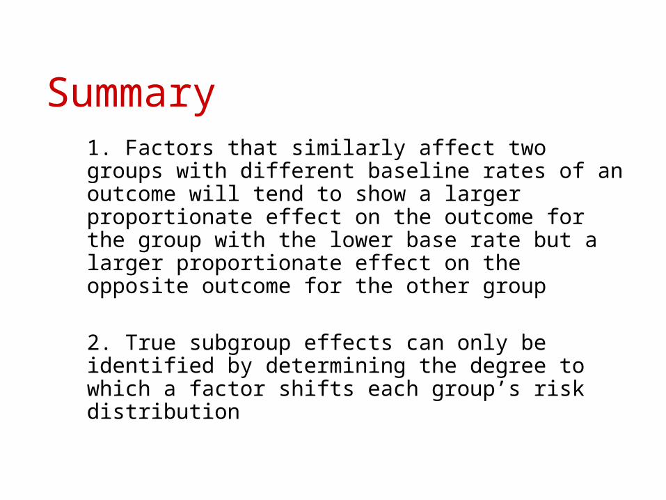
Summary 1. Factors that similarly affect two groups with different baseline rates of an outcome will tend to show a larger proportionate effect on the outcome for the group with the lower base rate but a larger proportionate effect on the opposite outcome for the other group

2. True subgroup effects can only be identified by determining the degree to which a factor shifts each group’s risk distribution

References

Measuring Health Disparities page on jpscanlan.com – especially the Solutions tab

Scanlan’s Rule page on jpscanlan.com – especially the Subgroup Effects tab

Can We Actually Measure Health Disparities? (Chance 2006)

Race and Mortality (Society 2000)

Divining Difference (Chance 1994)

An illogical expectation

There exists a tendency to regard it as somehow normal that a factor that similarly affects two groups’ susceptibilities to an outcome will cause the same proportionate change in the outcome rates for each group and to regard anything else as a differential effect (subgroup effect, interaction)

One reason the expectation is illogical

Where two groups have different base rates of experiencing an outcome, a factor that has the same proportionate effect on each group’s rate of experiencing the outcome necessarily has a different proportionate effect on each group’s rate of avoiding the outcome

E.g., Group A (10/90); Group B (20/80)

A logical expectation A factor that similarly affects two groups

with different baseline rates of an outcome will tend to show a larger proportionate effect on the outcome for the group with the lower base rate but a larger proportionate effect on the opposite outcome for the other group

Why is that logical?

Interpretive Rule 1/Scanlan’s Rule 1

When two groups differ in their susceptibility to an outcome, the rarer the outcome, the greater tends to be the relative difference in experiencing it and the smaller tends to be the relative difference in avoiding it.

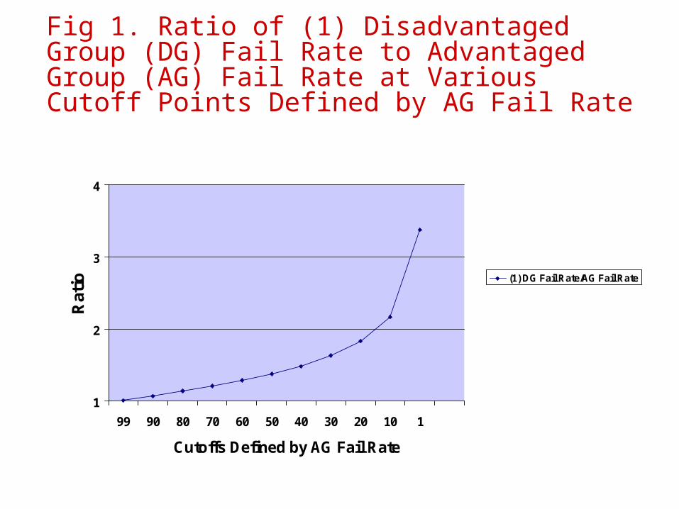
Fig 1. Ratio of (1) Disadvantaged Group (DG) Fail Rate to Advantaged Group (AG) Fail Rate at Various Cutoff Points Defined by AG Fail Rate

1

2

3

4

99 90 80 70 60 50 40 30 20 10 1

Cutoffs Defined by AG Fail Rate

Rat

io (1) DG Fail Rate/AG Fail Rate

Fig. 2. Ratios of (1) DG Fail Rate to AG Fail Rate and (2) AG Pass Rate to DG Pass Rate at Various Cutoff Points Defined by AG Fail Rate

1

2

3

4

99 90 80 70 60 50 40 30 20 10 1

Cutoffs Defined by AG Fail Rate

Rat

ios (1) DG Fail Rate/AG Fail Rate

(2) AG Pass Rate/DG Pass Rate

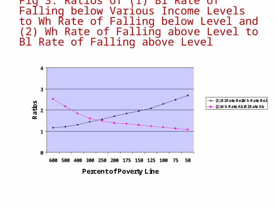
Fig 3. Ratios of (1) Bl Rate of Falling below Various Income Levels to Wh Rate of Falling below Level and (2) Wh Rate of Falling above Level to Bl Rate of Falling above Level

0

1

2

3

4

600 500 400 300 250 200 175 150 125 100 75 50

Percent of Poverty Line

Ra

tio

s (1) Bl Rate Bel/Wh Rate Bel

(2) Wh Rate Ab/Bl Rate Ab

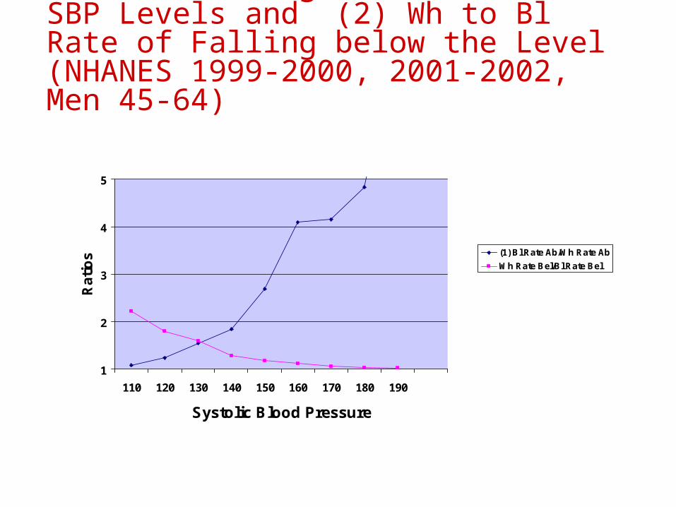
Fig. 4. Ratio of (1) Bl to Wh Rate of Falling above Various SBP Levels and (2) Wh to Bl Rate of Falling below the Level (NHANES 1999-2000, 2001-2002, Men 45-64)

1

2

3

4

5

110 120 130 140 150 160 170 180 190

Systolic Blood Pressure

Ra

tio

s (1) Bl Rate Ab/Wh Rate Ab

Wh Rate Bel/Bl Rate Bel

Implications of SR1 As an adverse becomes less prevalent relative difference in experiencing it

tend to increase while relative differences in avoiding it tend to decline (e.g., test failure, poverty, hypertension, mortality).

Relative differences in adverse outcomes tend to be larger among advantaged subpopulations while relative differences in favorable outcomes tend to be smaller among such subpopulations (e.g. race differences in health outcomes among the college-educated, race and SES differences in health outcomes among the young, SES differences in health outcomes among British Civil servants)

Factors that decrease/increase the prevalence of an outcome will tend to have greater proportionate effect on group with lower base rate but greater proportionate effect on the opposite outcome for the other group

Problems Arising from SR1 When we observe standard patterns of changes

in differences between group rates as prevalence of an outcome changes, how do we determine whether the difference between the groups’ situations actually changed in a meaningful way and how do we quantify the difference at each point in time (in a way that is unaffected by overall prevalence)?

How do we identify genuine differential effects?

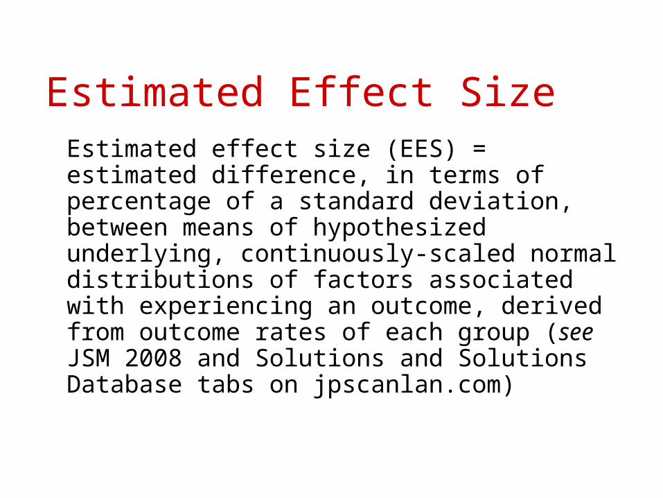
Estimated Effect SizeEstimated effect size (EES) = estimated difference, in terms of percentage of a standard deviation, between means of hypothesized underlying, continuously-scaled normal distributions of factors associated with experiencing an outcome, derived from outcome rates of each group (see JSM 2008 and Solutions and Solutions Database tabs on jpscanlan.com)

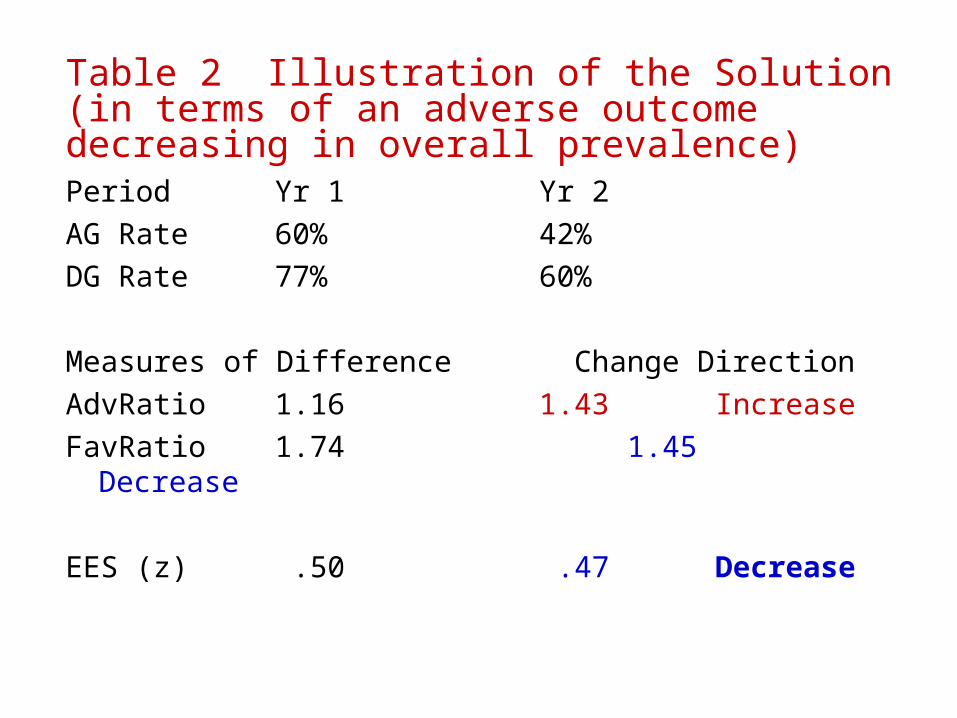
Table 2 Illustration of the Solution (in terms of an adverse outcome decreasing in overall prevalence)Period Yr 1 Yr 2

AG Rate 60% 42%

DG Rate 77% 60%

Measures of Difference Change Direction

AdvRatio1.16 1.43 Increase

FavRatio 1.74 1.45 Decrease

EES (z) .50 .47 Decrease

Illustrations from Two Perspectives

Perspective 1: Identifying/evaluating differential effects of factor on two groups

Perspective 2: Comparing the size of the difference between the rates of two groups according to the presence or absence of a factor

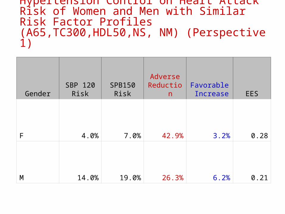
Table 3. Comparison of Effects of Hypertension Control on Heart Attack Risk of Women and Men with Similar Risk Factor Profiles (A65,TC300,HDL50,NS, NM) (Perspective 1)

GenderSBP 120

RiskSPB150

RiskAdverse

ReductionFavorable Increase EES

F 4.0% 7.0% 42.9% 3.2% 0.28

M 14.0% 19.0% 26.3% 6.2% 0.21

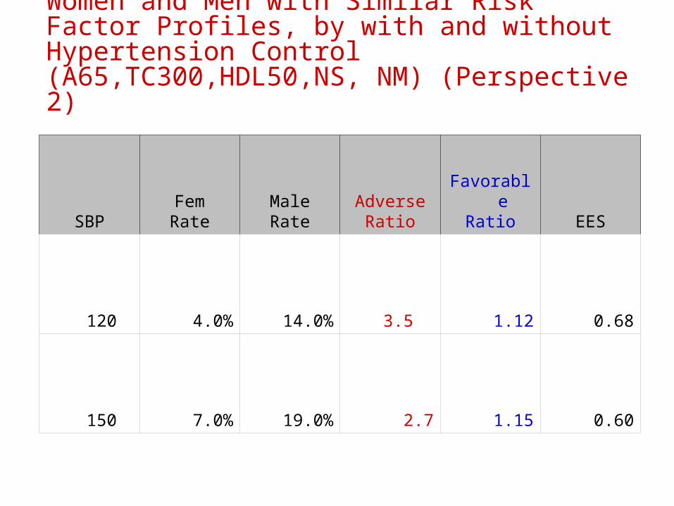
Table 4. Comparison of Gender Differences in Heart Attack Risk for Women and Men with Similar Risk Factor Profiles, by with and without Hypertension Control (A65,TC300,HDL50,NS, NM) (Perspective 2)

SBPFemRate

MaleRate

AdverseRatio

FavorableRatio EES

120 4.0% 14.0% 3.5 1.12 0.68

150 7.0% 19.0% 2.7 1.15 0.60

Table 5: Comparison of Black-White Difference in Lung Cancer among <11 and > 29 Cig Per Day (Haimon NEJM 2006) (Perspective 2)

Cig/Day White Rate Black RateAdverse

RatioFavorable

Ratio EES

<11 0.7% 2.2% 3.1 1.015 0.44

>29 3.1% 5.4% 1.7 1.024 0.26

Table 6. Comparison of Effects of Decreasing Smoking from >29 to <11 Cig Per Day on Whites and Blacks (Haimon NEJM 2006) (Perspective 1) (cor. 9/20/14)

Race <11 CPD >29 CPDAdverse Reduction

FavorableIncrease EES

W 0.7% 3.1% 77.2% 2.5% 0.60

B 2.2% 5.9% 63.4% 4.0% 0.42

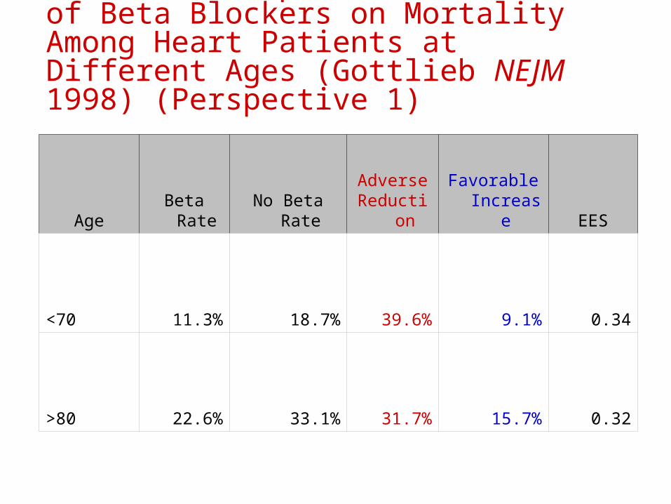
Table 7. Comparison of Effects of Beta Blockers on Mortality Among Heart Patients at Different Ages (Gottlieb NEJM 1998) (Perspective 1)

Age Beta Rate No Beta RateAdverse

ReductionFavorable

Increase EES

<70 11.3% 18.7% 39.6% 9.1% 0.34

>80 22.6% 33.1% 31.7% 15.7% 0.32

Table 8. Comparison of Age Differences in Mortality Among Patients Treated and Not Treated with Beta Blockers (Gottlieb NEJM 1998) (Perspective 2)

Treatment Status <70 Rate >80 Rate

Adverse Ratio

Favorable Ratio EES

Beta 11.3% 22.6% 2.0 1.15 0.48

NoBeta 18.7% 33.1% 1.8 1.22 0.45

Issues Contrary literature regarding the patterns

Clinical significance issue

Statistical significance issues Re spurious patterns Re solutions approach

Absolute minimum issue