STAFF EXHIBIT 20

RA- H4Sg'7NUREG-1576

EPA 402-B-04-001ANTIS PB2004-105421

Multi-Agency Ndooia

Laboratory Analytical Protocols ManualVolume I: Chapters 1 - 9 and Appendices A- E

OEEDby Applicmnt/Ucensee Interveor;

S , 0thr

011w

tDENIR• on1 Witness/Panel_____',.t•onTacen: ADMIITiED REJECTED •WrFDIAr

SDOCKETED

~USNRC

La oratober Anayta -Prto ol Manuapm

RULEMAKINGS AND

ADJUDICATIONS STAFF

Docket No. 40-8838-ML

IFEb-Aplcnioso nwo

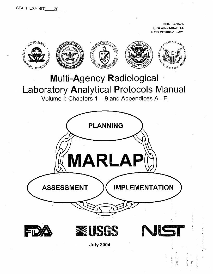
STAFF EXHIBIT 20

NUREG-1576EPA 402-B-04-001A

NTIS PB2004-105421

ED STIý

Multi-Agency RadiologicalLaboratory Analytical Protocols

Volume I: Chapters 1 - 9 and AppendicesManual

A-E

"W5 I I u&IRV'"S'sAML NNrML E

i %j LSr

July 2004

ABSTRACT

The Multi-Agency Radiological Laboratory Analytical Protocols (MARLAP) manual providesguidance for the planning, implementation, and assessment of projects that require the laboratoryanalysis of radionuclides. MARLAP's basic goal is to provide guidance for project planners,managers, and laboratory personnel to ensure that radioanalytical laboratory data will meet aproject's or program's data requirements. To attain this goal, the manual offers a framework fornational consistency in the form of a performance-based approach for meeting data requirementsthat is scientifically rigorous and flexible enough to be applied to a diversity of projects andprograms. The guidance in MARLAP is designed to help ensure the generation of radioanalyticaldata of known quality, appropriate for its intended use. Examples of data collection activities thatMARLAP supports include site characterization, site cleanup and compliance demonstration,decommissioning of nuclear facilities, emergency response, remedial and removal actions,effluent monitoring of licensed facilities, environmental site monitoring, background studies, andwaste management activities.

MARLAP is organized into two parts. Part I, intended primarily for project planners andmanagers, provides the basic framework of the directed planning process as it applies to projectsrequiring radioanalytical data for decision making. The nine chapters in Part I offerrecommendations and guidance on project planning, key issues to be considered during thedevelopment of analytical protocol specifications, developing measurement quality objectives,project. planning documents and their significance, obtaining laboratory services, selecting andapplying analytical methods, evaluating methods and laboratories, verifying and validatingradiochemical data, and assessing data quality. Part II is intended primarily for laboratorypersonnel. Its eleven chapters provide detailed guidance on field sampling issues that affectlaboratory measurements, sample receipt and tracking, sample preparation in the laboratory,sample dissolution, chemical separation techniques, instrumentation for measuring radionuclides,data acquisition, reduction, and reporting, waste management, laboratory quality control,measurement uncertainty, and detection and quantification capability. Seven appendices providecomplementary information and additional details on specific topics.

MARLAP was developed by a workgroup that included representatives from the U.S. Environ-mental Protection Agency (EPA), Department of Energy (DOE), Department of Defense (DOD),Department of Homeland Security (DHS), Nuclear Regulatory Commission (NRC), NationalInstitute of Standards and Technology (NIST), U.S. Geological Survey (USGS), and Food andDrug Administration (FDA), and from the Commonwealth of Kentucky and the State ofCalifornia.

JULY 2004 III MARLAP

CONTENTS

PageA b stract ......... . .. . .. .. ... .. .. .......... .. . .. .. .. . ........... ....... .. .. Iv

Forew ord g.. nts............................................................ V

Acknowledgments.. ......... .... VI

Contents of Appendices .................................................... xxxvi

L ist of Figures ........ ...................................................... X LI

L ist of T ables .............................................................. X LV

Acronym s and Abbreviations .................................................. XLIX

U nit C onversion Factors ...................................................... LVII

1 Introduction to M A RLA P ................................................... 1-11.1 O verview ............................................................ 1-11.2 Purpose of the M anual .................................................. 1-21.3 Use and Scope of the M anual ............................................ 1-31.4 Key MARLAP Concepts and Terminology .................................. 1-4

1.4.1 D ata L ife C ycle ................................................. 1-41.4.2 Directed Planning Process ......................................... 1-51.4.3 Performance-Based Approach ...................................... 1-51.4.4 A nalytical Process ................................................ 1-61.4.5 A nalytical Protocol .................... ......................... 1-71.4.6 A nalytical M ethod ............................................... 1-71.4.7 U ncertainty and Error ............................................. 1-71.4.8 Precision, Bias, and Accuracy ...................................... 1-91.4.9 Performance Objectives; Data Quality Objectives and Measurement Quality

O bjectives .................................................... 1-101.4.10 Analytical Protocol Specifications .................................. 1-111.4.11 The A ssessm ent Phase ........................................... 1-11

1.5 The M ARLA P Process ........................... ...................... 1-121.6 Structure of the M anual ................................................ 1-13

1.6.1 O verview of Part I .............................................. 1-161.6.2 O verview of PartI1 ............................................... 1-171.6.3 Overview of the Appendices ...................................... 1-18

1.7 R eferences. .......................................................... 1-19

JULY 2004 XI MARLAP

Contents

Page

2 Project Planning Process .................................................... 2-12.1 Introduction ................................................ .. 2-12.2 The Importance of Directed Project Planning ................................ 2-22.3 Directed Project Planning Processes ....................................... 2-3

2.3.1 A Graded Approach to Project Planning .............................. 2-42.3.2 Guidance on Directed Planning Processes ............................. 2-42.3.3 Elements of Directed Planning Processes ............................. 2-5

2.4 The Project Planning Team ............................................... 2-62.4.1 Team Representation ............................................. 2-72.4.2 The Radioanalytical Specialists ..................................... 2-7

2.5 Directed Planning Process and Role of the Radioanalytical Specialists ............ 2-82.5.1 State the Problem .... ...... ....... ...... 2-112.5.2 Identify the D ecision ............................................ 2-12

2.5.2.1 Define the Action Level ....................................... 2-122.5.2.2 Identify Inputs to the Decision .................................. 2-132.5.2.3 Define the Decision Boundaries ................................ 2-132.5.2.4 Define the Scale of the Decision ................................ 2-14

2.5.3 Specify the Decision Rule and the Tolerable Decision Error Rates ........ 2-142.5.4 Optimize the Strategy for Obtaining Data ............................ 2-15

2.5.4.1 Analytical Protocol Specifications ............................... 2-162.5.4.2 Measurement Quality Objectives ............................... 2-16

2.6 Results of the Directed Planning Process .................................. 2-172.6.1 Output Required by the Radioanalytical Laboratory: The Analytical Protocol

Specifications .................................................. 2-182.6.2 Chain of Custody ............................................... 2-19

2.7 Project Planning and Project Implementation and Assessment ................. 2-192.7.1 Documenting the Planning Process ................................. 2-192.7.2 Obtaining Analytical Services ..................................... 2-202.7.3 Selecting Analytical Protocols ..................................... 2-202.7.4 A ssessm ent Plans ............................................... 2-21

2.7.4.1 D ata V erification ............................................ 2-212.7.4.2 Data V alidation ....................................... 2-222.7.4.3 Data Quality Assessm ent ...................................... 2-22

2.8 Summary of Recommendations .......................................... 2-222.9 R eferences .......................................................... 2-23

3 Key Analytical Planning Issues and Developing Analytical Protocol Specifications ...... 3-13.1 Introduction .......................................................... 3-13.2 Overview of the Analytical Process ........................................ 3-23.3 General Analytical Planning Issues ........................................ 3-2

MARLAP XII JULY 2004

Contents

Page

3.3.1 D evelop A nalyte List ............................................. 3-33.3.2 Identify Concentration Ranges ...................................... 3-53.3.3 Identify and Characterize Matrices of Concern ......................... 3-53.3.4 Determine Relationships Among the Radionuclides of Concern ........... 3-63.3.5 Determine Available Project Resources and Deadlines ................... 3-73.3.6 Refine Analyte List and M atrix List ................................. 3-73.3.7 Method Performance Characteristics and Measurement Quality Objectives ... 3-7

3.3.7.1 Develop MQOs for Select Method Performance Characteristics ........ 3-93.3.7.2 The Role of MQOs in the Protocol Selection and Evaluation Process ... 3-143.3.7.3 The Role of MQOs in the Project's Data Evaluation Process .......... 3-14

3.3.8 Determine Any Limitations on Analytical Options ..................... 3-153.3.8.1 Gam m a Spectrom etry ........................................ 3-163.3.8.2 Gross Alpha and Beta Analyses ................................. 3-163.3.8.3 Radiochemical Nuclide-Specific Analysis ......................... 3-17

3.3.9 Determine M ethod Availability ................................... 3-173.3.10 Determine the Type and Frequency of, and Evaluation Criteria for, Quality

C ontrol Sam ples ............................................... 3-173.3.11 Determine Sample Tracking and Custody Requirements ................ 3-183.3.12 Determine Data Reporting Requirements ............................ 3-19

3.4 M atrix-Specific Analytical Planning Issues ................................. 3-203 .4 .1 Solids ............................................... ......... 3-2 1

3.4.1.1 Removal of Unwanted M aterials ................................ 3-213.4.1.2 Homogenization. and Subsampling .............................. 3-213.4.1.3 Sam ple D issolution .......................................... 3-22

3.4.2 L iquids ....................................................... 3-223.4.3 Filters and W ipes ............................................... 3-23

3.5 Assembling the Analytical Protocol Specifications ........................... 3-233.6 Level of Protocol Performance Demonstration .............................. 3-243.7 Project Plan D ocum ents ................................................ 3-243.8 Summary of Recommendations .......................................... 3-273.9 R eferences .......................................................... 3-27Attachment 3A: M easurement Uncertainty .................................... 3-29

3A .1 Introduction ........................................ ............ 3-293A .2 Analogy: Political Polling ........................................ 3-293A.3 M easurem ent Uncertainty ........................................ 3-303A.4 Sources of Measurement Uncertainty ............................... 3-313A.5 Uncertainty Propagation .......................................... 3-323A .6 R eferences .................................................... 3-32

Attachment 3B: Analyte Detection .......................................... 3-333B .1 Introduction ..................................................... 3-33

JULY 2004 X1II MARLAP

Contents

Page

3B .2 The Critical V alue .............................................. 3-343B.3 The M inimum Detectable Value ................................... 3-353B.4 Sources of Confusion ............................................ 3-363B.5 Implem entation Difficulties ....................................... 3-37

4 Project Plan Docum ents ................................. ............ 4-14 .1 Introduction ................................... ...................... 4-14.2 The Importance of Project Plan Documents ................................. 4-24.3 A Graded Approach to Project Plan Documents ............................. 4-34.4 Structure of Project Plan Documents ...................................... 4-3

4.4.1 Guidance on Project Plan Documents ................................ 4-44.4.2 Approaches to Project Plan Documents .............................. 4-5

4.5 Elements of Project Plan Documents ....................................... 4-64.5.1 Content of Project Plan Documents .................................. 4-64.5.2 Plan Documents Integration ........................................ ; 4-94.5.3 Plan Content for Small Projects .................................... 4-9

4.6 Linking the Project Plan Documents and the Project Planning Process ........... 4-104.6.1 Planning Process Report ......................... ............... 4-144.6.2 D ata A ssessm ent ............................................... 4-15

4.6.2.1 D ata V erification ............................................ 4-154.6.2.2 D ata V alidation ............................................. 4-154.6.2.3 Data Quality Assessm ent ...................................... 4-16

4.7 Summary of Recommendations .......................................... 4-174.8 R eferences .......................................................... 4-17

5 Obtaining Laboratory Services ................................................ 5-15.1 Introduction .......................................................... 5-15.2 Importance of Writing a Technical and Contractual Specification Document ....... 5-25.3 Statement of Work- Technical Requirements ............................... 5-2

5.3.1 A nalytes .... ................................................... 5-35 .3 .2 M atrix .......................................................... 5-35.3.3 M easurement Quality Objectives .................................... 5-35.3.4 Unique Analytical Process Requirements .............................. 5-45.3.5 Quality Control Samples and Participation in External Performance Evaluation

P rogram s ...................................................... 5-45.3.6 Laboratory Radiological Holding and Turnaround Times ................. 5-55.3.7 Number of Samples and Schedule .................................. 5-55.3.8 Q uality System .................................................. 5-65.3.9 Laboratory's Proposed M ethods .................................... 5-6

5.4 Request for Proposal-Generic Contractual Requirements ................... 5-7-

MARLAP XIV JULY 2004

Contents

Page

5.4.1 Sample Management ............5.4.2 Licenses, Permits and Environmental Re

5.4.2.1 Licenses .....................5.4.2.2 Environmental and Transportation R

egulat

egula5.4.3 Data Reporting and Communications ......

5.4.3.1 Data Deliverables ...................5.4.3.2 Software Verification and Control ......5.4.3.3 Problem Notification and Communication5.4.3.4 Status Reports ....................

5.4.4 Sample Re-Analysis Requirements ........5.4.5 Subcontracted Analyses .................

5.5 Laboratory Selection and Qualification Criteria .

5.5.1 Technical Proposal Evaluation ...........5.5.1.1 Scoring and Evaluation Scheme .......5.5.1.2 Scoring Elements ...................

5.5.2 Pre-Award Proficiency Evaluation ........5.5.3 Pre-Award Assessments and Audits .........

5.6 Summary of Recommendations .................5.7 R eferences ..............................

5.7.1 Cited References ......................5.7.2 Other Sources .........................

6 Selection and Application of an Analytical Method .....6.1 Introduction ................................6.2 M ethod Definition ...........................

ions ....................tions .............................

....................." .............

............

............

............

............

............

............

............

............

............

............

............

............

............

5-75-85-85-85-95-9

5-105-105-115-115-115-115-125-125-135-145-155-155-165-165-16

6.3 Life Cycle of M ethod Application ...........................6.4 Generic Considerations for Method Development and Selection ...6.5 Project-Specific Considerations for Method Selection I ..........

6.5.1 Matrix and Analyte Identification .....................6.5.1.1 M atrices ......................................6.5.1.2. Analytes and Potential Interferences ...............

6.5.2 Process Know ledge ..................................6.5.3 Radiological Holding and Turnaround Times ............6.5.4 Unique Process Specifications ........................6.5.5 Measurement Quality Objectives ..................

6.5.5.1 Method Uncertainty ........................6.5.5.2 Quantification Capability .........................6.5.5.3 D etection Capability ............................6.5.5.4 Applicable Analyte Concentration Range ............6.5.5.5 M ethod Specificity ..............................

6-16-16-36-56-9

6-116-116-116-146-146-156-166-176-176-186-196-206-20

JULY 2004 XV MARLAP

Contents

Page

6.5.5.6 M ethod Ruggedness .............................6.5.5.7 Bias Considerations ..............................

6.6 M ethod V alidation ........................................6.6.1 General M ethod Validation ...........................6.6.2 Project Method Validation Protocol ....................6.6.3 Tiered Approach to Project Method Validation ............

6.6.3.1 Existing Methods Requiring No Additional Validation6.6.3.2 Routine Methods Having No Project Method Validation6.6.3.3 Use of a Validated Method for Similar Matrices ........6.6.3.4 New Application of a Validated Method ...............6.6.3.5 Newly Developed or Adapted Methods ...............

6.6.4 Testing for B ias ....................................6.6.4.1 A bsolute B ias ...................................6.6.4.2 R elative B ias ....................................

6.6.5 Project Method Validation Documentation ................6.7 Analyst Qualifications and Demonstrated Proficiency ...........6.8 Method Control ...................................6.9 Continued Performance Assessment...................6.10 Documentation To Be Sent to the Project Manager ...........6.11 Summary of Recommendations ...........................6.12 - R eferences ...........................................Attachment 6A: Bias-Testing Procedure ... ......................

6A .1 Introduction ............ ...........................6A .2 T he T est ...........................................6A.3 Bias Tests at Multiple Concentrations ....................

7 Evaluating Methods and Laboratories .............................7.1 Introduction ............. .........................7.2 Evaluation of Proposed Analytical Methods ....................

7.2.1 Documentation of Required Method Performance .........7.2.1.1 Method Validation Documentation ..................7.2.1.2 Internal Quality Control or External PE Program Reports7.2.1.3 Method Experience, Previous Projects, and Clients .....7.2.1.4 Internal and External Quality Assurance Assessments ...

7.2.2 Performance Requirements of the SOW-Analytical Protocol7.2.2.1 Matrix and Analyte Identification ...................7.2.2.2 Radiological Holding and Turnaround Times ..........7.2.2.3 Unique Processing Specifications ...................7.2.2.4 Measurement Quality Objectives ....................7.2.2.5 Bias Considerations ..............................

6-216-216-226-246-256-266-286-286-286-296-306-316-316-326-326-326-336-346-356-366-366-396-396-396-42

.............. 7-1.......... ... 7-1............. 7-2............. 7-2............. 7-3............. 7-4............. 7-5............. 7-5Specifications . 7-5............. 7-6

......... .... 7-7

......... .... 7-8. ............ 7-8............ 7-13

MARLAP XVI JULY 2004

Contents

Page

7.3 Initial Evaluation of a Laboratory ........................................ 7-157.3.1 Review of Quality System Documents .............................. 7-157.3.2 Adequacy of Facilities, Instrumentation, and Staff Levels .............. 7-177.3.3 Review of Applicable Prior W ork .................................. 7-177.3.4 Review of General Laboratory Performance .......................... 7-18

7.3.4.1 Review of Internal QC Results ................................. 7-187.3.4.2 External PE Program Results ................................... 7-197.3.4.3 Internal and External Quality Assessment Reports .................. 7-20

7.3.5 Initial A udit ................................................... 7-207.4 Ongoing Evaluation of the Laboratory's Performance ........................ 7-20

7.4.1 Quantitative Measures of Quality ............................. 7-217.4.1.1 M Q O Com pliance ........................................... 7-227.4.1.2 O ther Param eters ............................................ 7-27

7.4.2 Operational A spects ............................................. 7-287.4.2.1 D esk A udits ................................................ 7-287.4.2.2 O nsite A udits ............................................... 7-30

7.5 Summary of Recommendations .......................................... 7-327.6 R eferences .......................................................... 7-33

8 Radiochemical Data Verification and Validation ................................ 8-18.1 Introduction .......................................................... 8-18.2 Data A ssessm ent Process ................................................ 8-2

8.2.1 Planning Phase of the Data Life Cycle ................................ 8-28.2.2 Implementation Phase of the Data Life Cycle .......................... 8-3

8.2.2.1 Project O bjectives ............................................ 8-38.2.2.2 Documenting Project Activities ................................. 8-48.2.2.3 Quality Assurance/Quality Control .............................. 8-4

8.2.3 Assessment Phase of the Data Life Cycle ............................. 8-58.3 Validation Plan ........... .............. 8-7

8.3.1 Technical and Quality Objectives of the Project ....................... 8-88.3.2 V alidation T ests ................................................. 8-98.3.3 D ata Q ualifiers .................................................. 8-98.3.4 Reporting and Documentation ..................................... 8-10

8.4 Other Essential Elements for Data Validation ............................... 8-118.4.1 Statem ent of W ork .............................................. 8-118.4.2 Verified Data Deliverables ........................................ 8-12

8.5 Data Vcrification and Validation Process .................................. 8-128.5.1 The Sample Handling and Analysis System .......................... 8-13

8.5.1.1 Sam ple D escriptors .......................................... 8-148.5.1.2 A liquant Size ............................................... 8-15

JULY 2004 XVII MARLAP

Contents

Page

8.5.1.3 Dates of Sample Collection, Preparation, and Analysis .............. 8-168.5.1.4 Preservation ................................................. 8-168.5.1.5 T racking ................................................... 8-178.5.1.6 T raceability ................................................ 8-178.5.1.7 QC Types and Linkages ....................................... 8-188.5.1.8 Chem ical Separation (Yield) ................................... 8-188.5.1.9 Self-A bsorption ............................................. 8-198.5.1.10 Efficiency, Calibration Curves, and Instrument Background ......... 8-198.5.1.11 Spectrom etry Resolution ..................................... 8-208.5.1.12 Dilution and Correction Factors ................................ 8-208.5.1.13 Counts and Count Time (Duration) ............................. 8-218.5.1.14 Result of Measurement, Uncertainty, Minimum Detectable Concentration,

and U nits ..................................................... 8-2 18.5.2 Quality Control Sam ples ......................................... 8-22

8.5.2.1 M ethod B lank ............................................... 8-238.5.2.2 Laboratory Control Samples ................................... 8-238.5.2.3 Laboratory Replicates ........................................ 8-248.5.2.4 Matrix Spikes and Matrix Spike Duplicates ....................... 8-24

8.5.3 Tests of Detection and Unusual Uncertainty .......................... 8-25.8.5.3.1 D etection ................ ................................. 8-25

8.5.3.2 D etection Capability ............................ * ............. 8-268.5.3.3 Large or Unusual Uncertainty .......................... ....... 8-27

8.5.4 Final Qualification and Reporting .................................. 8-278.6 V alidation R eport ...................................................... 8-298.7 Summary of Recommendations .......................................... 8-318.8 B ibliography ......................................................... 8-3 1

9 Data Quality A ssessm ent .............. ............. ....................... 9-19.1 Introduction .......................................................... 9-19.2 A ssessm ent Phase ..................................................... 9-29.3 Graded Approach to Assessment .......................................... 9-39.4 The Data Quality Assessment Team ....................................... 9-39.5 Data Quality Assessm ent Plan ............................................ 9-49.6 Data Quality Assessment Process .................................... 9-5

9.6.1 Review of Project Documents ............................... ...... 9-79.6.1.1 The Project DQOs and M QOs .................................... 9-79.6.1.2 The D Q A Plan ............................................... 9-89.6.1.3 Summary of the DQA Review ................................... 9-8

9.6.2 Sample Representativeness ........................................ 9-99.6.2.1 Review of the Sampling Plan .................................... 9-9

MARLAP XVIII JULY 2004

Contents

Page

9.6.2.2 Sampling Plan Implementation ..............9.6.2.3 Data Considerations .......................

9.6.3 Data A ccuracy ..............................9.6.3.1 Review of the Analytical Plan ...............9.6.3.2 Analytical Plan Implementation .............

9.6.4 Decisions and Tolerable Error Rates .............9.6.4.1 Statistical Evaluation of Data ...............9.6.4.2 Evaluation of Decision Error Rates ..........

9.7 Data Quality Assessment Report .......................9.8 Summary of Recommendations .......................9.9 R eferences .......................................

9.9.1 Cited Sources ...............................9.9.2 Other Sources ...............................

. . . . . . . . . .

. . . . . . . . . .

. . . . . . . . . .

. . . . . . . . . .

. . . . . . . . . .

. . . . . . . . . .

. . . . . . . . . .. . . . . . . . . .. . . . . . . . . .. . . . . . . . . .. . . . . . . . . .

9-129-139-149-189-199-219-219-249-259-269-279-279-27

Volume II

10 Field and Sampling Issues That Affect Laboratory Measurements ...Part A : Generic Issues ......................................10.1 Introduction .........................................10.2 Field Sampling Plan: Non-Matrix-Specific Issues ..... ......

10.2.1 Determination of Analytical Sample Size ..............10.2.2 Field Equipment and Supply Needs ...................10.2.3 Selection of Sample Containers ......................

10.2.3.1 Container Material ......................10.2.3.2 Container Opening and Closure ................10.2.3.3 Sealing Containers ..........................10.2.3.4 Precleaned and Extra Containers ...............

10.2.4 Container Label and Sample Identification Code ........10.2.5 Field Data Documentation ..........................10.2.6 Field Tracking, Custody, and Shipment Forms ..........10.2.7 Chain of Custody .................................10.2.8 Field Quality Control .............. ...............10.2.9 Decontamination of Field Equipment .................10.2.10 Packing and Shipping ............................10.2.11 Worker Health and Safety Plan .....................

10.2.11.1 Physical Hazards .......................10.2.11.2 Biohazards ..............................

......... 10-1

......... 10-1

......... 10-1

......... 10-3

......... 10-3

......... 10-3

......... 10-4

......... 10-4

......... 10-5

......... 10-5

......... 10-5

......... 10-6

......... 10-7

......... 10-8

......... 10-9

........ 10-10

........ 10-10

........ 10-11

........ 10-12

.... ..... 10-13

........ 10-15Part B: Matrix-Specific Issues That Impact Field Sample Collection, Processing, and

Preservation ........................................................ 10-1610.3 Liquid Sam ples .................................................. 10-17

JULY 2004 XIX MARLAP

Contents

10.3.1 Liquid Sam pling M ethods ....................................... 10-1810.3.2 Liquid Sample Preparation: Filtration .............................. 10-18

10.3.2.1 Example of Guidance for Ground-Water Sample Filtration ....... 10-1910.3.2.2 Filters ............................

10.3.3 Field Preservation of Liquid Samples .........10.3.3.1 Sample Acidification ................10.3.3.2 Non-Acid Preservation Techniques .....

10.3.4 Liquid Samples: Special Cases ..............10.3.4.1 Radon-222 in W ater .................10.3.4.1 M ilk ..... ........................

10.3.5 Nonaqueous Liquids and Mixtures ............10 .4 S olids .....................................

10 .4 .1 Soils ...................................10.4.1.1 Soil Sample Preparation ..............10.4.1.2 Sample Ashing ....................

10.4.2 Sedim ents ..............................10.4.3 O ther Solids ............................

10.4.3.1 Structural M aterials .................

....................

....................

....................

................I ...

....................

....................

....................

..........I .........

....................

....................

....I ...............

....................

10-2110-2210-2210-2310-2510-2510-2610-2610-2810-2910-2910-3010-3010-31

....... 10-3110.4.3.2 Biota: Samples of Plant and Animal Products ..................

10.5 A ir Sam pling ....................................................10.5.1 Sampler Components and Operation ..............................10.5.2 Filter Selection Based on Destructive Versus Nondestructive Analysis ....10.5.3 Sample Preservation and Storage .................................10.5.4 Special Cases: Collection of Gaseous and Volatile Air Contaminants ...

10.5.4.1 R adioiodines ...........................................10.5.4 .2 G ases .................................. ..............10.5.4.3 Tritium Air Sam pling .....................................10.5.4.4 Radon Sampling in Air ...................................

10.6 Wipe Sampling for Assessing Surface Contamination ....................10.6.1 Sample Collection M ethods .....................................

10.6.1.1 D ry W ipes .............................................10.6.1.2 W et W ipes .............................................

10.6.2 Sam ple H andling .............................................10.6.3 Analytical Considerations for Wipe Material Selection ................

10.7 R eferences ......................................................

10-3110-3410-3410-3510-3610-3610-3610-3710-3810-3910-4110-4210-4210-4310-4410-4410-45

11 Sample Receipt, Inspection, and Tracking .............11.1 Introduction ...............................11.2 General Considerations ...................

11.2.1 Communication Before Sample Receipt ......

.... ...... 11-1. . . . . . . . . . . . . . . . . . . 11-1. . . . . . . . . ..-.. . . . . . . 1. . . . . . . . . . . . . . . . . . . 11-1

MARLAP XX JULY 2004

Contents

Page

11.2.2 Standard Operating Procedures .................11.2.3 Laboratory License ...........................11.2.4 Sample Chain-of-Custody .....................

11.3 Sam ple R eceipt ................................11.3.1 Package Receipt ..... ...................11.3.2 Radiological Surveying .......................11.3.3 Corrective A ction ................. ..........

11.4 Sam ple Inspection ..............................11.4.1 Physical Integrity of Package and Sample Containers11.4.2 Sample Identity Confirmation ..................11.4.3 Confirmation of Field Preservation ..............11.4.4 Presence of Hazardous Materials ................11.4.5 Corrective Action ............................

11.5 Laboratory Sample Tracking ......................11.5.1 Sam ple Log-In ..............................11.5.2 Sample Tracking During Analyses ...............11.5.3 Storage of Sam ples ............ I...............

11.6 R eferences ....................................

... . .. . . . ... . . . .. . .. 11-3

....... .. . . . . . . .... 1 1-4. . . . . . . . . . . . . . . . . . . 1 1-4

...........

...........

...........

...........

...........

...........

...........

...........

...........

...........

...........

...........

...........

11-511-511-611-811-811-811-911-911-9

11-1011-1111-1l11-1111-1211-13

12 Laboratory Sample Preparation .....................................12.1 Introduction ..............................................12.2 General Guidance for Sample Preparation ........................

12.2.1 Potential Sample Losses During Preparation .................12.2.1.1 Losses as Dust or Particulates ........................12.2.1.2 Losses Through Volatilization .......................12.2.1.3 Losses Due to Reactions Between Sample and Container..

12.2.2 Contamination from Sources in the Laboratory ................12.2.2.1 Airborne Contamination ...........................12.2.2.2 Contamination of Reagents .........................12.2.2.3 Contamination of Glassware and Equipment ...........12.2.2.4 Contamination of Facilities .........................

12.2.3 Cleaning of Labware, Glassware, and Equipment ..............12.2.3.1 Labware and Glassware ............................12.2.3.2 Equipm ent ......................................

12.3 Solid Sam ples ............................................12.3.1 G eneral Procedures ......................................

12.3.1.1 Exclusion of M aterial ..............................

....... 12-1

....... 12-1

....... 12-2

....... 12-2....... 12-2....... 12-3....... 12-5....... 12-6....... 12-7....... 12-7....... 12-8....... 12-8....... 12-8....... 1-2-8...... 12-10..... . 12-12...... 12-12

...... 12-14

...... 12-14...... 12-23...... 12-24

12.3.1.212.3.1.312.3.1.4

Principles of Heating Techniques for Sample PretreatmentObtaining a Constant W eight ........................Subsam pling .....................................

JULY 2004 XXI MARLAP

Contents

Page

12.3.2 Soil/Sedim ent Sam ples ......................................... 12-2712.3.2 .1 " S oils .................................................. 12-2812.3.2.2 Sedim ents .............................................. 12-28

12.3.3 B iota Sam ples ................................................ 12-2812.3.3.1 F ood .................................................. 12-2912.3.3.2. V egetation ............................................. 12-2912.3.3.3 B one and Tissue .......................................... 12-30

12.3.4 O ther Sam ples ................................................ 12-3012 .4 F ilters .......................................................... 12 -3012.5 W ipe Sam ples ................................................... 12-3112.6 Liquid Sam ples .................................................. 12-32

12.6.1 Conductivity ........................................... 12-3212.6.2 Turbidity ..................................................... 12-3212.6.3 Filtration .................................................... 12-3312.6.4 A queous Liquids .............................................. 12-3312.6.5 Nonaqueous Liquids ...................................... 12-3412.6.6 M ixtures ..................................................... 12-35

12.6.6.1 Liquid-Liquid M ixtures ................................... 12-3512.6.6.2 Liquid-Solid Mixtures ............................... 12-35

12.7 G ases .......................................................... 12-3612.8 B ioassay . ............................. ......................... 12-3612.9 References ................................ ..... .. 12-37

12.9.1 C ited Sources ................................................. 12-3712.9.2 Other Sources .......................................... 12-43

13 Sam ple D issolution ...................................................... 13-113.1 Introduction ...................................................... 13-113.2 The Chem istry of Dissolution ........................................ 13-2

13.2.1 Solubility and the Solubility Product Constant, Ksp .................... 13-213.2.2 Chemical Exchange, Decomposition, and Simple Rearrangement Reactions . 13-313.2.3 Oxidation-Reduction Processes .................................... 13-413.2.4 C om plexation .................................................. 13-513.2.5 Equilibrium: Carriers and Tracers .................................. 13-6

13.3 Fusion Techniques ................................................. 13-613.3.1 Alkali-M etal Hydroxide Fusions ................................... 13-913.3.2 Boron Fusions . .-................ .. . ...... 13-1113.3.3 Fluoride Fusions . ...................................... 13-1213.3.4 Sodium Hydroxide Fusion ....................................... 13-12

1-3.4 W et Ashing and Acid Dissolution Techniques .......................... 13-1213.4.1 A cids and O xidants ............................................ 13-13

MARLAP XXIT JULY 2004

Contents

Pa2e

13.4.2 Acid Digestion Bombs ....................................... 13-2013.5 M icrow ave D igestion .............................................. 13-21

13.5.1 Focused Open-Vessel Systems ................................... 13-2113.5.2 Low-Pressure, Closed-Vessel Systems ............................. 13-2213.5.3 High-Pressure, Closed-Vessel Systems ............................. 13-22

13.6 Verification of Total Dissolution ..................................... 13-2313.7 Special M atrix Considerations ....................................... 13-23

13.7.1 Liquid Sam ples ............................................... 13-2313.7.2 Solid Sam ples ................................................ 13-2413.7.3 -F ilters ....................................................... 13-2413.7.4 W ipe Sam ples ................................................ 13-24

13.8 Comparison of Total Dissolution and Acid Leaching ..................... 13-2513.9 R eferences ...................................................... 13-27

13.9.1 Cited References .............................................. 13-2713.9.2 O ther Sources ................................................. 13-29

14 Separation Techniques ....................... d ............................ 14-114.1 Introduction ...................................................... 14-114.2 Oxidation-Reduction Processes ....................................... 14-2

14.2.1 Introduction ...................... ......... 14-214.2.2 Oxidation-Reduction Reactions ............... .................... 14-314.2.3 Com mon Oxidation States ........................................ 14-614.2.4 Oxidation State in Solution ...................................... 14-1014.2.5 Common Oxidizing and Reducing Agents .......................... 14-1114.2.6 Oxidation State and Radiochemical Analysis ..................... 14-13

14.3 C om plexation .................................................... 14-1814.3.1 Introduction .................................................. 14-1814.3.2 C helates ..................................................... 14-2014.3.3 The Formation (Stability) Constant ................................ 14-2214.3.4 Complexation and Radiochemical Analysis ......................... 14-23

14.3.4.1 Extraction of Laboratory Samples and Ores .................... 14-2314.3.4.2 Separation by Solvent Extraction and Ion-Exchange Chromatography 14-2314.3.4.3 Formation and Dissolution of Precipitates ..................... 14-2414.3.4.4 Stabilization of Ions in Solution ............................. 14-2414.3.4.5 Detection and Determination ................................ 14-25

14.4 Solvent Extraction ................................................ 14r2514.4.1 Extraction Principles ..... ........................ ............. 14-2514.4.2 D istribution Coefficient ......................................... 14-2614.4.3 Extraction Technique ...... ..................................... 14-2714.4.4 Solvent Extraction and Radiochemical Analysis ...................... 14-30

JULY 2004 XXIII MARLAP

Contents

Page

14.4.5 Solid-Phase Extraction .......................................... 14-3214.4.5.1 Extraction Chromatography Columns ........................ 14-3314.4.5.2 Extraction M embranes .................................... 14-34

14.4.6 Advantages and Disadvantages of Solvent Extraction ................. 14-3514.4.6.1 Advantages of Liquid-Liquid Solvent Extraction ............... 14-3514.4.6.2 Disadvantages of Liquid-Liquid Solvent Extraction ............. 14-3514.4.6.3 Advantages of Solid-Phase Extraction Media .................. 14-3514.4.6.4 Disadvantages of Solid-Phase Extraction Media ................ 14-36

14.5 Volatilization and Distillation ....................................... 14-3614.5.1 Introduction .................................................. 14-3614.5.2 V olatilization Principles ........................................ 14-3614.5.3 D istillation Principles .......................................... 14-3814.5.4 Separations in Radiochemical Analysis ............................. 14-3914.5.5 Advantages and Disadvantages of Volatilization ..................... 14-40

14.5.5.1 A dvantages .......................................... ... 14-4014.5.5.2 D isadvantages .......................................... 14-40

14.6 Electrodeposition ................................................. 14-4114.6.1 Electrodeposition Principles ..................................... 14-4114.6.2 Separation of Radionuclides ..................................... 14-4214.6.3 Preparation of Counting Sources .................................. 14-4314.6.4 Advantages and Disadvantages of Electrodeposition .................. 14-43

14.6.4.1 A dvantages ............................................. 14-4314.6.4.2 D isadvantages ............................................ 14-43

14.7 Chrom atography .................................................. 14-4414.7.1 Chromatographic Principles ....................................... 14-4414.7.2 Gas-Liquid and Liquid-Liquid Phase Chromatography ................. 14-4514.7.3 Adsorption Chromatography ..................................... 14-4514.7.4 Ion-Exchange Chromatography ................................... 14-46

14.7.4.1 Principles of Ion Exchange ................................ 14-4614.7.4.2 Resins ......................... 14-48

14.7.5 Affinity Chromatography ........................................ 14-5414.7.6 Gel-Filtration Chromatography ................................... 14-5414.7.7 Chromatographic Laboratory Methods ............................. 14-5514.7.8 Advantages and Disadvantages of Chromatographic Systems ........... 14-56

14.7.8.1 Advantages ............................................ 14-5614.7.8.2 Disadvantages ........ ............................. 14-56

14.8 Precipitation and Coprecipitation .......................... ......... 14-5614.8.114.8.214.8.3

Introduction ...................................................S olu tion s . . . . . . . . . . .. . .. .. . . . . . .. .. . . .. . .. . . . . . . . . .. . . . . . .. .P recipitation ..................................................

14-5614-5714-59

MARLAP XXIV JULY 2004

Contents

14.8.3.114.8.3.214.8.3.3

Solubility and the Solubility Product Constant, Kp.............Factors Affecting Precipitation .............................Optimum Precipitation Conditions......................

14.8.4 C oprecipitation ................................................14.8.4.1 Coprecipitation Processes .................................14.8.4.2 W ater as an Im purity .....................................14.8.4.3 Postprecipitation ........................................14.8.4.4 Coprecipitation M ethods ..................................

14.8.5 C olloidal Precipitates ...........................................14.8.6 Separation of Precipitates .........................................14.8.7 Advantages and Disadvantages of Precipitation and Coprecipitation ......

14.8.7.1 A dvantages .............................................14.8.7.2 D isadvantages ..........................................

14.9 C arriers and Tracers ...............................................14.9.1 Introduction ..................................................14.9.2 C arriers ......................................................

14.9.2.1 Isotopic C arriers ..........................................14.9.2.2 N onisotopic Carriers ............. ........................

Page

14-5914-6414-6914-6914-7014-7414-7414-7514-7814-8114-8214-8214-8214-8214-8214-8314-8314-84

14.9.2.3 Common Carriers14.9.2.4 Holdback Carriers .....................14.9.2.5 Yield of Isotopic Carriers ................

14.9.3 T racers ....................................14.9.3.1 Characteristics of Tracers ................14.9.3.2 Coprecipitation ........................14.9.3.3 Deposition on Nonmetallic Solids ..........14.9.3.4 Radiocolloid Formation ................14.9.3.5 Distribution (Partition) Behavior ..........14.9.3.6 V aporization ..........................14.9.3.7 Oxidation and Reduction ................

14.10 Analysis of Specific Radionuclides .................14.10.1 Basic Principles of Chemical Equilibrium ......14.10.2 O xidation State ...........................14.10.3 H ydrolysis ...............................14.10.4 Polym erization ............................14.10.5 Com plexation ............................14.10.6 Radiocolloid Interference ..................14.10.7 Isotope Dilution Analysis ...................14.10.8 Masking and Demasking .................14.10.9 Review of Specific Radionuclides .............

14.10.9.1 A m ericium ...........................

.... 14-85

.... 14-89

.... 14-89

.... 14-90

.... 14-92

.... 14-93

.... 14-93

.... 14-94

.... 14-95

.... 14-95

.... 14-96

.... 14-97

.... 14-97

... 14-100

... 14-100

... 14-102

... 14-103

... 14-103

... 14-104... 14-105... 14-109... 14-109

MARLAPJULY 2004 XXV

Contents

Page

14.10.9.2 C arbon ............................................... 14-11414.10.9.3 C esium ...... ......................................... 14-11614.10.9.4 C obalt .................. .............................. 14-11914.10.9.5 Iodineptuniu ........................... .............. 14-12514.10.9.6 N eptunium ..... ........................ .............. 14-13214.10.9.7 N ickel .... ......................................... 14-13614.10.9.8 Plutonium .............................................. 14-13914.10.9.9 R adium ..... ........................................ 14-14814.10.9.10 Strontium ........................................... 14-15514.10.9.11 Sulfur and Phosphorus ..... .............................. 14-16014.10.9.12 Technetium ............................................. 14-16314.10.9.13 Thorium ...... ........................................ 14-16914.10.9.14 T ritium ..... ......................................... 14-17514.10.9.15 U ranium ..... ........................................ 14-18014.10.9.16 Zirconium .......................................... 14-19114.10.9.17 Progeny of Uranium and Thorium .......................... 14-198

14.11 R eferences ..................................................... 14-20 114.12 Selected Bibliography ............................................ 14-218

14.12.1 Inorganic and Analytical Chemistry ............................ 14-21814.12.2 General Radiochemistry ..................................... 14-21914.12.3 Radiochemical Methods of Separation .......................... 14-21914.12.4 Radionuclides ............................................. 14-22014.12.5 Separation M ethods ......................................... 14-222

Attachment 14A Radioactive Decay and Equilibrium .......................... 14-22314A.1 Radioactive Equilibrium ....................................... 14-223

14A .1.1 Secular Equilibrium ..................................... 14-22314A.1.2 Transient Equilibrium ................................... 14-22514A .1.3 N o Equilibrium ........................................ 14-22614A.1.4 Summary of Radioactive Equilibria .......................... 14-227

14A.1.5 Supported and Unsupported Radioactive Equilibria ................ 14-22814A.2 Effects of Radioactive Equilibria on Measurement Uncertainty ......... 14-229

14A .2.1 Issue ................................................. 14-22914A.2.2 Discussion ...................................... 14-22914A.2.3 Examples of Isotopic Distribution: Natural, Enriched, and Depleted

U ranium .............................................. 14-23 114A .3 R eferences .................................................. 14-232

15 Quantification of Radionuclides ............................................ 15-115.1 Introduction ............................................. .. 15-115.2 Instrum ent Calibrations ............................................. 15-2

MARLAP XXVI JULY 2004

Contents

Page

15.2.115.2.215.2.315.2.4

C alibration Standards ...........................................Congruence of Calibration and Test-Source Geometry ..................Calibration and Test-Source Homogeneity ...........................Self-Absorption, Attenuation, and Scattering Considerations for Source

15-315-315-5

Preparations ... . . . . . . . . . . ... . . . . . . . . . . . . . . . . . . . . . . . . . . . . . . . . . . . . . 1 5 -515.2.5 Calibration Uncertainty .................

15.3 Methods of Source Preparation ..............15.3.1 Electrodeposition ......................15.3.2 Precipitation/Coprecipitation .............15.3.3 Evaporation ..........................15.3.4 Thermal Volatilization/Sublimation ........15.3.5 Special Source M atrices .................

15.3.5.1 Radioactive Gases ...............15.3.5.2 A irFilters ......................15.3.5.3 Sw ipes ........................

15.4 Alpha Detection Methods ..................15.4.1 Introduction ...........................

.......................... 15-7

.................... ...... 15-8

.... . .. . .......... ....... 15-8

. . . . . . . . . . . . . . . . . . . . . . . . 15 -1 1

.................. ..... 15-12

........................ 15-15

........................ 15-16

........................ 15-16

........................ 15-17

. . . . . . . . . . . . . . . . . . . . . . . . 15 -18

. . . . . . . . . . . . . . . . . . . . . . . . 15 -18

. . . . . . . . . . . . . . . . . . . . . . . . 15 -1815.4.2 Gas Proportional Counting ................................

15.4.2.1 Detector Requirements and Characteristics .....................15.4.2.2 Calibration and Test Source/Preparation ......................15.4.2.3 D etector Calibration .....................................15.4.2.4 Troubleshooting .........................................

15.4.3 Solid-State D etectors ............................................15.4.3.1 Detector Requirements and Characteristics .................15.4.3.2 Calibration- and Test-Source Preparation .....................15.4.3.3 D etector Calibration ......................... ............15.4.3.4 Troubleshooting .........................................15.4.3.5 Detector or Detector Chamber Contamination .................15.4.3.6 Degraded Spectrum ......................................

15.4.4 Fluorescent D etectors ...........................................15.4.4.1 Zinc Sulfide ............................................15.4.4.2 Calibration- and Test-Source Preparation ..................15.4.4.3 Detector Calibration ........... ........ .............15.4.4.4 Troubleshooting ..................................

15.4.5 Photon Electron Rejecting Alpha Liquid Scintillation (PERALSO) .......15.4.5.1 Detector Requirements and Characteristics ....................15.4.5.2 Calibration- and Test-Source Preparation .....................15.4.5.3 D etector Calibration ......................................15.4.5.4 Q uench ................................................15.4.5.5 A vailable C ocktails ......................................

15-2015-2015-2515-2515-2715-2915-3015-3315-3315-3415-3515-3715-3815-3815-4015-4115-4115-4215-4215-4415-4515-4515-46

JULY 2004 XXVII MARLAP

Contents

Page

15.4.5.6 Troubleshooting ......................................... 15-4615.5 Beta D etection M ethods ............................................ 15-46

15.5.1 Introduction ................................................... 15-4615.5.2 Gas Proportional Counting/Geiger-Mueller Tube Counting ............. 15-49

15.5.2.1 Detector Requirements and Characteristics .................... 15-4915.5.2.2 Calibration- and Test-Source Preparation ..................... 15-5315.5.2.3 Detector Calibration ................. .................... 15-5415.5.2.4. Troubleshooting ......................................... 15-57

15.5.3 Liquid Scintillation ............................................ 15-5715.5.3.1 Detector Requirements and Characteristics .................... 15-58i 5.5.3.2 Calibration- and Test-Source Preparation ..................... 15-6115.5.3.3 D etector Calibration ...................................... 15-6215.5.3.4 Troubleshooting ......................................... 15-68

15.6 Gamma Detection M ethods ......................................... 15-6815.6.1 Sample Preparation Techniques ............................... .. 15-70

15.6.1.1 C ontainers ............................................. 15-7115.6.1.2 G ases ................................................. 15-7 115.6.1.3 L iquids ................................................ 1,5-7215.6.1.4 Solids ................................ ................ 15-72

15.6.2 Sodium Iodide Detector ......................................... 15-7315.6.2.1 Detector Requirements and Characteristics .................... 15-7315.6.2.2 Operating Voltage ....................................... 15-7615.6.2.3 Shielding .............................................. 15-7615.6.2.4 B ackground ............................................ 15-7615.6.2.5 D etector Calibration ...................................... 15-7715.6.2.6 Troubleshooting ......................................... 15-77

15.6.3 High Purity Germ anium ............ ............... I .............. 15-7815.6.3.1 Detector Requirements and Characteristics .................... 15-7815.6.3.2 Gamma Spectrometer Calibration ........................... 15-8215.6.3.3 Troubleshooting ......................................... 15-84

15.6.4 Extended-Range Germanium Detectors ............................ 15-8815.6.4.1 Detector Requirements and Characteristics .................... 15-8915.6.4.2 D etector Calibration ...................................... 15-8915.6.4.3 Troubleshooting ......................................... 15-90

15.6.5 Special Techniques for Radiation Detection ......................... 15-9015.6.5.1 Other Gamma Detection Systems ........................... 15-9015.6.5.2 Coincidence Counting .................................... 15-9115.6.5.3 Anti-Coincidence Counting ................................ 15-93

15.7 Specialized Analytical Techniques ......... .......................... 15-9415.7.1 Kinetic Phosphorescence Analysis by Laser (KPA) ................... 15-94

MARLAP XXVIII JULY 2004

Contents

Page

15.7.2 M ass Spectrom etry ............................................. 15-9515.7.2.1 Inductively Coupled Plasma-Mass Spectrometry ............... 15-9615.7.2.2 Thermal Ionization Mass Spectrometry ....................... 15-9915.7.2.3 Accelerator M ass Spectrometry .................... ....... 15-100

15.8 R eferences ...................................................... 15-10 115.8.1 Cited R eferences ....... . .................................. 15-10115.8.2 O ther Sources ................................................ 15-115

16 Data Acquisition, Reduction, and Reporting for Nuclear Counting Instrumentation .... 16-116.1 Introduction ...................................................... 16-1

.16.2 D ata A cquisition .................................................. 16-216.2.1 Generic Counting Parameter Selection .............................. 16-3

16.2.1.1 Counting Duration ........................................ 16-416.2.1.2 Counting Geom etry ..................... .................. 16-516.2.1.3 Softw are .................................................. 16-5

16.2.2 Basic Data Reduction Calculations ................................. 16-616.3 Data Reduction on Spectrometry Systems .............................. 16-8

16.3.1 Gamm a-Ray Spectrometry ........................................ 16-916.3.1.1 Peak Search or Identification ................................. 16-1016.3.1.2 Singlet/M ultiplet Peaks .................................... 16-1316.3.1.3 Definition of Peak Centroid and Energy ........................ 16-1416.3.1.4 Peak W idth Determination ................................... 16-1516.3.1.5 Peak Area Determination .................................. 16-1716.3.1.6 Calibration Reference File ............ .................... 16-1916.3.1.7 Activity and Concentration ................................ 16-2016.3.1.8 Summing Considerations .................................. 16-2116.3.1.9 Uncertainty Calculation ..................................... 16-22

16.3.2 A lpha Spectrom etry ............................................ 16-2316.3.2.1 Radiochemical Yield .................................... 16-27.16.3.2.2 Uncertainty Calculation .................................... 16-28

16.3.3 Liquid Scintillation Spectrometry ................................. 16-2916.3.3.1 Overview of Liquid Scintillation Counting ...................... 16-2916.3.3.2 Liquid Scintillation Spectra ................................ 16-2916.3.3.3 3 Pulse Characteristics ..................................... 16-2916.3.3.4 Coincidence Circuitry .................................... 16-3016.3.3.5 Q uenching ............................................. 16-3016.3.3.6 Lum inescence ........................................... 16-3116.3.3.7 Test-Source V ials ........................................ 16-3116.3.3.8 Data Reduction for Liquid Scintillation Counting ............... 16-31

16.4 Data Reduction on Non-Spectrometry Systems .......................... 16-32

JULY 2004 XXIX MARLAP

Contents

Page

16.5 Internal Review of Data by Laboratory Personnel ........................ 16-3616.5.1 Prim ary R eview ............................................... 16-3716.5.2 Secondary Review ............................................. 16-37

16.6 R eporting Results ................................................. 16-3816.6.1 Sample and Analysis Method Identification ......................... 16-3816.6.2 Units and Radionuclide Identification .......................... 16-3816.6.3 Values, Uncertainty, and Significant Figures ......................... 16-39

16.7 Data Reporting Packages ........................................... 16-3916.8 Electronic Data Deliverables ........................................ 16-4116.9 R eferences ...................................................... 16-4 1

16.9.1 Cited R eferences .............................................. 16-4116.9.2 O ther Sources ................................................. 16-44

17 Waste Management in a Radioanalytical Laboratory ......................... 17-117.1 Introduction ...................................................... 17-117.2 Types of Laboratory W astes ......................................... 17-117.3 W aste M anagement Program ......................................... 17-2

17.3.1 Program Integration ............................................. 17-317.3.2 Staff Involvem ent ............................... ................ 17-3

17.4 W aste M inim ization ................................................ 17-317.5 W aste Characterization ............................................. 17-617.6 Specific Waste Management Requirements ............................. 17-6

17.6.1 Sample/W aste Exemptions ....................................... 17-917.6.2 Storage ................................................ 17-9

17.6.2.1 Container Requirements ................................ 17-1017.6.2.2 Labeling Requirements ................................ 17-1017.6.2.3 Tim e Constraints ........................................... 17-1117.6.2.4 M onitoring Requirem ents ................................... 17-11

17.6.3 T reatm ent .................................................... 17-1217.6.4 D isposal ..................................................... 17-12

17.7 Contents of a Laboratory Waste Management Plan/Certification Plan ........ 17-1317.7.1 Laboratory W aste Management Plan ............................... 17-1317.7.2 Waste Certification Plan/Program ................................ 17-14

17.8 U seful W eb Sites ................................................. 17-1517.9 R eferences ...................................................... 17-17

17.9.1 Cited R eferences .............................................. 17-1717.9.2 O ther Sources ................................................. 17-17

MARLAP XXX JULY 2004

Contents

Page

Volume III

18 Laboratory Q uality Control ................................................ 18-118.1 Introduction ...... ...................... ........................ 18-1

18.1.1 Organization of Chapter .......................................... 18-218.1.2 F orm at ....................................................... 18-2

18.2 Q uality C ontrol ................................................... 18-318.3 Evaluation of Performance Indicators .................................. 18-3

18.3.1 Importance of Evaluating Performance Indicators ...................... 18-318.3.2 Statistical Means of Evaluating Performance Indicators - Control Charts .. 18-518.3.3 Tolerance Lim its ........... .............................. 18-718.3.4 M easurem ent Uncertainty ............. ........................... 18-8

18.4 Radiochemistry Performance Indicators ......... ...................... 18-918.4.1 M ethod and Reagent Blank ....................................... 18-918.4.2 Laboratory Replicates ........................................... 18-1318.4.3 Laboratory Control Samples, Matrix Spikes, and Matrix Spike Duplicates . 18-1618.4.4 Certified Reference M aterials .................................... 18-1818.4.5 Chem ical/Tracer Y ield ................... ...................... 18-21

18.5 Instrumentation Performance Indicators ............................... 18-2418.5.1 Instrument Background Measurements .......................... .. 18-2418.5.2 Efficiency Calibrations ......................................... 18-2618.5.3 Spectrom etry System s .......................................... 18-29

18.5.3.1 Energy Calibrations ...................................... 18-2918.5.3.2 Peak Resolution and Tailing ............................... 18-32

18.5.4 Gas Proportional System s ....................................... 18-3618.5.4.1 V oltage Plateaus ......................................... 18-3618.5.4.2 Self-Absorption, Backscatter, and Crosstalk .................. 18-37

18.5.5 Liquid Scintillation ............................................ 18-3818.5.6 Summary Guidance on Instrument Calibration, Background,

and Q uality C ontrol ............................................... 18-4018.5.6.1 Gas Proportional Counting Systems ......................... 18-4218.5.6.2 Gamma-Ray Detectors and Spectrometry Systems .............. 18-4518.5.6.3 Alpha Detector and Spectrometry Systems .................... 18-4918.5.6.4 Liquid Scintillation System s ............................... 18-51

18.5.7 Non-Nuclear Instrumentation ................................ 18-531.8.6 Related Concerns .................. ... 18-54

18.6.1 D etection Capability ..... ............................ ......... 18-5418.6.2 Radioactive Equilibrium ........................................ 18-5418.6.3 H alf-L ife .............................. ...................... 18-5718.6.4 Interferences .................................................. 18-58

JULY 2004 XXXI MARLAP

Contents

Page

18.6.5 N egative R esults ........................... .................. 18-6018.6.6 B lind Sam ples ................................................ 18-6118.6.7 Calibration of Apparatus Used for Mass and Volume Measurements ...... 18-63

18.7 References ........................................... ... 18-6518.7.1 Cited Sources .......................................... 18-6518.7.2 Other Sources .......................................... 18-67

Attachment ISA: Control Charts ..................................... 1-6918A. 1 Introduction . .......................................... 18-6918A .2 X C harts ..................................................... 18-69

18A .3 X C harts ..................................................... 18-7218A .4 R C harts ..................................................... 18-7418A.5 Control Charts for Instrument Response ............................ 18-7518A .6 R eferences ................................................... 18-79

Attachment 18B: Statistical Tests for QC Results .............................. 18-8118B .1 Introduction ................................................... 18-81188.2 Tests for Excess Variance in the Instrument Response ................. 18-8118B.3 Instrument Background Measurements ............................. 18-88

18B.3.1 Detection of Background Variability ......................... 18-8818B.3.2 Comparing a Single Observation to Preset Limits ............... 18-9018B.3.3 Comparing the Results of Consecutive Measurements .......... 18-93

18B.4 N egative A ctivities ............................................. 18-9618B .5 R eferences .................................................... 18-96

19 M easurem ent Uncertainty ................................................. 19-119.1 O verview ........................................................ 19-119.2 The Need for Uncertainty Evaluation .................................. 19-119.3 Evaluating and Expressing Measurement Uncertainty ..................... 19-3

19.3.1 M easurement, Error, and Uncertainty ........................ ....... 19-319.3.2 The M easurement Process ........................................ 19-419.3.3 Analysis of M easurement Uncertainty ............................... 19-619.3.4 Corrections for Systematic Effects .................................. 19-719.3.5 Counting Uncertainty ...................................... 19-719.3.6 Expanded Uncertainty ............................................ 19-719.3.7 Significant Figures .............................................. 19-819.3.8 Reporting the Measurement Uncertainty ............................. 19-919.3.9 Recom m endations .............. .......... ................... 19-10

19.4 Procedures for Evaluating Uncertainty ............................ 19-1119.4.1 Identifying Sources of Uncertainty ............................ 19-1219.4.2 Evaluation of Standard Uncertainties ........................... 19-13

MARLAP XXXII JULY 2004

Contents

Page

19.4.2.1 Type A Evaluations .............................19.4.2.2 Type B Evaluations .............................

19.4.3 Combined Standard Uncertainty .......................19.4.3.1 Uncertainty Propagation Formula ..................19.4.3.2 Components of Uncertainty ......................19.4.3.3 Special Forms of the Uncertainty Propagation Formula.

19.4.4 The Estimated Covariance of Two Output Estimates .......19.4.5 Special Considerations for Nonlinear Models .............

19.4.5.1 Uncertainty Propagation for Nonlinear Models .......19.4.5.2 Bias due to Nonlinearity .........................

19.4.6 M onte Carlo M ethods ................................19.5 Radiation Measurement Uncertainty .......................

19.5.1 Radioactive D ecay ..................................19.5.2 Radiation Counting .................................

19.5.2.1 Binom ial M odel .................................19.5.2.2 Poisson Approximation ..........................

19.5.3 Count Time and Count Rate ..........................19.5.3.1 D ead T im e ....................................19.5.3.2 A Confidence Interval for the Count Rate ...........

19.5.4 Instrument Background . .............................19.5.5 Radiochem ical Blanks ...............................19.5.6 Counting Effi ciency .................................19.5.7 Radionuclide Half-Life ..............................19.5.8 Gamma-Ray Spectrometry ............................19.5 9 B alances ..........................................19.5.10 Pipets and Other Volumetric Apparatus ................19.5.11 Digital Displays and Rounding ....................19.5.12 Subsam pling ......................................19.5.13 The Standard Uncertainty for a Hypothetical Measurement .

19.6 R eferences ...........................................19.6.1 C ited Sources ......................................19.6.2 O ther Sources ......................................

Attachment 19A: Statistical Concepts and Terms ...................19A .1 Basic Concepts .....................................19A.2 Probability Distributions .............................

19A.2.1 Norm al Distributions ...........................19A.2.2 Log-normal Distributions ........................19A.2.3 Chi-squared Distributions .........................19A .2.4 T-D istributions ................................

.... 19-13... 19-16.... 19-20

.... 19-20

.... 19-24

.... 19-25

.... 19-26

.... 19-29

.... 19-29

.... 19-31

.... 19-34

.... 19-34

.... 19-34... 19-35

.... 19-35.... 19-36.... 19-38.... 19-39.... 19-40.... 19-41.... 19-42.... 19-43.... 19-47.... 19-48.... 19-48.... 19-52.... 19-54.... 19-55.... 19-56.... 19-58.... 19-58.... 19-61.... 19-63.... 19-63.... 19-66.... 19-67.... 19-68.... 19-69.... 19-70

19A.2.5 Rectangular Distributions . . . . . . . . . . . . . . . . . . . . . . . . . . . . . . . . . . . 19 -7 1

JULY 2004 XXXIII MARLAP

Contents

Page

19A.2.6 Trapezoidal and Triangular Distributions ....................... 19-7219A.2.7 Exponential Distributions ................................... 19-7319A.2.8 Binomial Distributions ...................................... 19-7319A.2.9 Poisson Distributions ....................... .............. 19-74

19A .3 R eferences ................................................... 19-76Attachment 19B: Example Calculations .............................. ...... 19-77

19B .1 O verview .................................................... 19-7719B.2 Sample Collection and Analysis ................................... 19-771913.3 The M easurem ent M odel ........................................ 19-7819B.4 The Combined Standard Uncertainty ............................... 19-80

Attachment 19C: Multicomponent Measurement Models ........................ 19-8319C .1 Introduction .................................................. 19-8319C.2 The Covariance M atrix .......................................... 19-8319C.3 Least-Squares Regression ........................................ 19-8319C .4 R eferences ................. .................................. 19-84

Attachment 19D: Estimation of Coverage Factors ............................. 19-8519D .1 Introduction .................................................. 19-8519D .2 Procedure .................................................... 19-85

19D .2.1 Basis of Procedure ......................................... 19-8519D .2.2 A ssum ptions ............................................. 19-8519D.2.3 Effective Degrees of Freedom ................................ 19-8619D.2.4 Coverage Factor ..... ................................ 19-87

19D.3 Poisson Counting Uncertainty .................................... 19-8819D .4 R eferences ................................................... 19-91

Attachment 19E: Uncertainties of Mass and Volume Measurements ............... 19-9319E .1 Purpose ...................................................... 19-9319E.2 M ass M easurem ents ............................................ 19-93

19E.2.1 Considerations ............................................ 19-9319E.2.2 R epeatability ............... ............................. 19-9419E.2.3 Environm ental Factors ...................................... 19-9519E.2.4 C alibration ............................................... 19-9719E .2.5 Linearity ................................................. 19-9819E.2.6 Gain or Loss of M ass ....................................... 19-9819E.2.7 Air-Buoyancy Corrections ................................... 19-9919E.2.8 Combining the Components ................................ 19-103

19E.3 Volume M easurements ......................................... 19-10519E.3.1 First Approach ............................................ 19-10519E.3.2 Second Approach ......................................... 19-10819E.3.3 Third A pproach .......................................... 19-111

19E .4 R eferences .................................................. 19-111

MARLAP XXXIV JULY 2004

Contents

Page

20 Detection and Quantification Capabilities ......................................20 .1 O v erv iew ...........................................................

20.2 Concepts and D efinitions ............................................20.2.1 Analyte Detection Decisions .......................................

20-120-120-120-1

20.2.2 The Critical V alue .....................................20.2.3 The Blank .....................................20.2.4 The Minimum Detectable Concentration ....................20.2.6 Other Detection Terminologies ...........................20.2.7 The Minimum Quantifiable Concentration ..................

20.3 Recom m endations ........................................20.4 Calculation of Detection and Quantification Limits ..............

20.4.1 Calculation of the Critical Value ..........................20.4.1.1 Norm ally Distributed Signals ........................20.4.1.2 Poisson Counting .................................20.4.1.3 Batch Blanks ............. ....... ......

20.4.2 Calculation of the Minimum Detectable Concentration ........20.4.2.1 The Minimum Detectable Net Instrument Signal .........20.4.2.2 Normally Distributed Signals ........................20.4.2.3 Poisson Counting .................................20.4.2.4 More Conservative Approaches ......................20.4.2.5 Experimental Verification of the MDC ................

....... 20-3.

....... 20-5

....... 20-5........ 20-9....... 20-10...... 20-11...... 20-12...... 20-12...... 20-13...... 20-13...... 20-17...... 20-18...... 20-19...... 20-20...... 20-24...... 20-28...... 20-28

20.4.3 Calculation of the Minimum Quantifiable Concentration ...............20.5 R eferences ......................................................

20.5.1 C ited Sources .................................................20.5.2 O ther Sources .................................................

Attachment 20A: Low-Background Detection Issues ............................20A .1 O verview ....................................................20A.2 Calculation of the Critical Value ..................................

20A.2.1 Normally Distributed Signals ...............................20A .2.2 Poisson Counting ........... ............................

20A.3 Calculation of the Minimum Detectable Concentration ................20A.3.1 Normally Distributed Signals..........................20A .3.2 Poisson Counting ........................................

20A .4 R eferences ...................................................

20-2920-3320-3320-3520-3720-3720-3720-3720-3920-5320-5420-5820-62

Glossary ...................................................... End of each volum e

JULY 2004 XXXV MARLAP

Contents

Page

Appendices - Volume I

A Directed Planning Approaches .............................................. A-1A .1 Introduction . ..... ............................................... A -1A.2 Elements Common to Directed Planning Approaches ...................... A-2A.3 Data Quality Objectives Process ...................................... A-2A.4 Observational Approach .......................................... .. A-3A.5 Streamlined Approach for Environmental Restoration ..................... A-4A.6 Technical Project Planning ................................... ........ A-4A.7 Expedited Site Characterization ................ ...................... A-4A .8 V alue Engineering ................................................. A -5A .9 System s Engineering ............................................... A -6A. 10 Total Quality M anagement .......................................... A-6A .11 P artnering ........................................................ A -7A ,12 R eferences ....................................................... A -7

A.12.1 Data Quality Objectives .......................................... A-7A. 12.2 Observational Approach ......................................... A-9A. 12.3 Streamlined Approach for Environmental Restoration (Safer) ........... A-10A.12.4 Technical Project Planning ...................................... A-11A.12.5 Expedited Site Characterization ................................... A-1IA .12.6 V alue Engineering ............................................. A-12A .12.7 System s Engineering ........................................... A-13A.12.8 Total Quality M anagement ...................................... A-15A .12.9 Partnering .................................................... A -16

Appendix B The Data Quality Objectives Process .................................. B-1B .I Introduction ........................................................... B -1B.2 Overview of the DQO Process ............................................ B-2B.3 The Seven Steps of the DQO Process ...................................... B-3

B.3.1 DQO Process Step 1: State the Problem .............................. B-3B.3.2 DQO Process Step 2: Identify the Decision ............................ B-4B.3.3 DQO Process Step 3: Identify Inputs to the Decision .................... B-5B.3.4 DQO Process Step 4: Define the Study Boundaries ..................... B-6B.3.5 Outputs of DQO Process Steps 1 through 4 Lead Into Steps 5 through 7 ..... B-7B.3.6 DQO Process Step 5: Develop a Decision Rule ..................... B-.7B.3.7 DQO Process Step 6: Specify the Limits on Decision Errors .............. B-9B.3.8 DQO Process Step 7: Optimize the Design for Obtaining Data ........... B-22

B.4References .................................................. B-24Attachment BI: Decision Error Rates and the Gray Region for Decisions About

M ean Concentrations .................................................. B-26

MARLAP XXXVI JULY 2004

Contents

Page

B I.1 Introduction ................................................... B -26B1.2 The Region of Interest ........................................... B-26B1.3 Measurement Uncertainty at the Action Level ........................ B-26B1.4 The Null Hypothesis ............................................ B-29

Case 1: Assume the True Concentration is Over 1.0 ....................... B-30Case 2: Assume the True Concentration is 0.9 ........................... B-32

B1 .5 TheGray Region ............................................... B-32B 1.6 Sum m ary ..................................................... B -34

Attachment B2: Decision Error Rates and the Gray Region for Detection Decisions .... B-36B 2.1 Introduction ................................................... B -36B2.2 The DQO Process Applied to the Detection Limit Problem .............. B-36B2.3 Establish the Concentration Range of Interest ......................... B-37B2.4 Estimate the Measurement Variability when Measuring a Blank .......... B-41

Appendix C Measurement Quality Objectives for Method Uncertainty and Detection andQuantification Capability ................................................... C-1C .I Introduction .......................................................... C -1C .2 H ypothesis Testing ..................................................... C -1C.3 Development of MQOs for Analytical Protocol Selection ...................... C-3C.4The Role of the MQO for Method Uncertainty in Data Evaluation ............... C-9

C.4.1 Uncertainty Requirements at Various Concentrations .................... C-9C.4.2 Acceptance Criteria for Quality Control Samples ....................... C- 11

C .5R eferences .......................................................... C -17

Appendix D Content of Project Plan Documents .................................. D-1D .I Introduction ......................................................... D -1D.2Group A: Project M anagement .......................................... D-5

D.2.1 Project Management (Al): Title and Approval Sheet ................... D-5D.2.2 Project Management (A2): Table of Contents ......................... D-7D.2.3 Project Management (A3): Distribution List ......................... D-7D.2.4 Project Management (A4): Project/Task Organization .................. D-7D.2.5 Project Management (A5): Problem Definition/Background ............. D-8D.2.6 Project Management (A6): Project/Task Description ................... D-9D.2.7 Project Management (A7): Quality Objectives and Criteria for Measurement

D ata . . . . . . . . . . . . . . . . . . . . . .. . . . .. .. . . . . . . . . . . . . ... . .. . . .. .. . .. . . D -1 1D.2.7.1 Project's Quality Objectives ............................... D- 1ID.2.7.2 Specifying Measurement Quality Objectives ................... D-12D.2.7.3 Relation between the Project DQOs, MQOs, and QC Requirements D-13

D.2.8 Project Management (A8): Special Training Requirements/Certification ... D-13D.2.9 Project Management (A9): Documentation and Record ................ D-13

JULY 2004 XXXVII MARLAP

Contents

Page

D.3Group B: Measurement/Data Acquisition ................................. D-14D.3.1 Measurement/Data Acquisition (B1): Sampling Process Design ......... D-15D.3.2 Measurement/Data Acquisition (B2): Sampling Methods Requirements ... D-16D.3.3 Measurement/Data Acquisition (B3): Sample Handling and Custody

Requirements ...................... * '............... D-18D.3.4 Measurement/Data Acquisition (B4): Analytical Methods Requirements .. D-19D.3.5 Measurement/Data Acquisition (B5): Quality Control Requirements ..... D-21D.3.6 Measurement/Data Acquisition (B6): Instrument/Equipment Testing, Inspection,

and Maintenance Requirements .............. ................ D-22D.3.7 Measurement/Data Acquisition (B7): Instrument Calibration and Frequency D-23D.3.8 Measurement/Data Acquisition (B8): Inspection/Acceptance Requirements for

Supplies and Consumables ...................................... D-23D.3.9 Measurement/Data Acquisition (B9): Data Acquisition Requirements for Non-

Direct M easurement Data ....................................... D-24D.3.10 Measurement/Data Acquisition (B 10): Data Management .............. D-25

D.4Group C: Assessment/Oversight ........................................ D-26D.4.1 Assessment/Oversight (Cl): Assessment and Response Actions ......... D-26D.4.2 Assessment/Oversight (C2): Reports to Management ................. D-27

D.5Group D: Data Validation and Usability ..................... ............. D-28D.5.1 Data Validation and Usability (Dl): Verification and Validation

R equirem ents ...................................................... D -28D.5.2 Data Validation and Usability (D2): Verification and Validation Methods . D-29

D .5.2.1 Data Verification ........................................ D-29D .5.2.2 Data V alidation ......................................... D -30

D.5.3 Data Validation and Usability (D3): Reconciliation with Data QualityO bjectives ...................................................... D -30

D .6R eferences .......................................................... D -3 1

Appendix E Contracting Laboratory Services .... ................................ E-1E .1 Introduction .......................................................... E -1E.2 Procurem ent of Services ................................................ E-4

E.2.1 Request for Approval of Proposed Procurement Action .................. E-5E.2.2 Types of Procurement M echanisms .................................. E-6

E.3 Request for Proposals- The Solicitation ................... ............... E-7E.3.1 M arket R esearch ................................................ E-8E.3.2 Period of C ontract ............................................... E-9E .3.3 Subcontracts .................................................... E-9

E.4 Proposal Requirem ents ................................................ E- 10E.4.1 RFP and Contract Information ..................................... E- 1IE .4.2 P ersonnel ..................................................... E -13

MARLAP XXXVIII JULY 2004

Contents

Page

E.4.3 Instrum entation ................................................ E-15E.4.3.1 Type, Number, and Age of Laboratory Instruments .............. E-16E.4.3.2 Service Contract .......................................... E-16

E.4.4 N arrative to Approach .............................. ............ E-16E.4.4.1 Analytical M ethods or Protocols ............................. E-16E.4.4.2 Meeting Contract Measurement Quality Objectives .............. E-17E.4.4.3 D ata Package ............................................ E-17E .4.4.4 Schedule ................................................ E-17E.4.4.5 Sample Storage and Disposal ................................ E-18

E.4.5 Q uality M anual ...... .......................................... E-18E.4.6 Licenses and Accreditations ....................................... E-19E .4.7 E xperience .................................................... E-20

E.4.7.1 Previous or Current Contracts ............................... E-20E.4.7.2 Quality of Performance .................................... E-20

E.5 Proposal Evaluation and Scoring Procedures ........................... E-21E.5.1 Evaluation Com m ittee ............................................ E-21E.5.2 Ground Rules - Questions ........................ E-22E.5.3 Scoring/Evaluating Scheme ....................................... E-22

E.5.3.1 Review of Technical Proposal and Quality Manual .............. E-23E.5.3.2 Review of Laboratory Accreditation ........................... E-25E.5.3.3 Review of Experience ..................................... E-25

E.5.4 Pre-Award Proficiency Samples ................................... E-25E.5.5 Pre-Award Audit ........................................ E-26E.5.6 Com parison of Prices ............................................ E-30E.5.7 Debriefing of Unsuccessful Vendors ................................ E-30

E .6 T he A w ard .......................................................... E -31E.7 For the Duration of the Contract ......................................... E-31

E.7.1 M anaging a Contract ............................................ E-32E.7.2 Responsibility of the Contractor ................................... E-32E.7.3 . Responsibility of the Agency ...................................... E-32E.7.4 Anomalies and Nonconformance ...................... ............ E-33E.7.5 Laboratory Assessment .......................................... E-33

E.7.5.1 Performance Testing and Quality Control Samples .............. E-33E.7.5.2 Laboratory Performance Evaluation Programs .................. E-34E.7.5.3 Laboratory Evaluations Performed During the Contract Period ..... E-35

E.8 Contract Com pletion ............................... ................... E-36E .9 R eferences ..................... ........... ......................... E -36

JULY 2004 XXXIX. MARLAP

Contents

Page

Appendices - Volume II

Appendix F Laboratory Subsampling ............................................ F-iF .1 Introduction .......................................................... F-iF.2 B asic C oncepts ........................................................ F-2F.3 Sources of M easurem ent Error ........................................... F-3

*F.3.1 Sam pling B ias .................................................. F-4F.3.2 Fundamental Error ........................................ F-5F.3.3 Grouping and Segregation Error .................................... F-6

F.4 Implementation of the Particulate Sampling Theory ........................... F-9F.4.1 The Fundamental Variance ....................................... F- 10F.4.2 Scenario 1 - Natural Radioactive Minerals ........................... F- 10F.4.3 Scenario 2 - Hot Particles ......................................... F-11F.4.4 Scenario 3 - Particle Surface Contamination ......................... F-13

F .5 Sum m ary ' ........ .................................................. F-15F .6 R eferences .......................................................... F-16

Appendices - Volume III

0 Statistical Tables ........................................................ G -1

MARLAP XL JULY 2004

Contents

Page

List of Figures

Figure 1.1 The data life cycle ................................................... 1-4Figure 1.2 Typical components of an analytical process ............... ............. 1-6Figure 1.3 The M ARLAP process ............................................. 1-14Figure 1.4 Key MARLAP terms and processes ........................... 1-15

Figure 3.1 Typical components of an analytical process .............................. 3-2Figure 3.2 Analytical protocol specifications ..................................... 3-25Figure 3.3 Example analytical protocol specifications .............................. 3-26Figure 3B.1 The critical value of the net signal ................................... 3-35

Figure 6.1 A nalytical process .................................................. 6-2Figure 6.2 M ethod application life cycle ......................................... 6-6Figure 6.3 Expanded Figure 6.2 addressing the laboratory's method evaluation process .... 6-7Figure 6.4 Relationship between level of laboratory effort, method validation level,'and degree

of assurance of method performance under the tiered approach to method validation ... 6-27

Figure 7.1 Considerations for the initial evaluation of a laboratory .................... 7-16

Figure 8.1 The assessm ent process .............................................. 8-5

Figure 9.1 Using physical samples to measure a characteristic of the populationrepresentatively . ......................................................... 9-10

Figure 9.2 Types of sampling and analytical errors ................................. 9-17

Volume II

Figure 10.1

Figure 11.1

Figure 12.1Figure 12.2

Figure 14.1Figure 14.2Figure 14.3

resins

JULY 2004

Example of chain-of-custody record ..... I ........................... 10-9

Overview of sample receipt, inspection, and tracking ..................... 11-2

Degree of error in laboratory sample preparation relative to other activities ... 12-1Laboratory sample preparation flowchart (for solid samples) .............. 12-13

Ethylene diamine tetraacetic acid (EDTA) ............................ 14-20C row n ethers ................................................... 14-2 1The behavior of elements in concentrated hydrochloric acid on cation-exchange. . . . . . . . . . . . . . . . . . . . . . . . . . . . . . . . . . . . . . . . . . . . . . . . . . . . . . . . . . . . . . . 14 -5 2

XLI MARLAP

Contents

Page

Figure 14.4 The behavior of elements in concentrated hydrochloric acid on anion-exchangeresin s . . . . . . . . . . . . . . . . . ... . . . . . . . . . . . . . . . . . . . . . . . . . . . . . . . . . . . . . . . . . . . . . 14 -5 3

Figure 14.5 The electrical double layer ......................................... 14-79Figure 14A.1 Decay chain for 238U .......................................... 14-224Figure 14A.2 Secular equilibrium of 2'°Pb/ 2'°Bi ................. ............... 14-225Figure 14A.3 Transient equilibrium of 95 Zr/ 9 5Nb ................................. 14-226Figure 14A.4 No equilibrium of 239U/239Np .................................... 14-227

Figure 15.1 Alpha plateau generated by a 210po source on a GP counter using P-10 gas ... 15-23Figure.15.2 Gas proportional counter self-absorption curve for 230Th ................. 15-28Figure 15.3 Beta plateau generated by a 9°Sr/Y source on a GP counter using P-10 gas ... 15-52Figure 15.4 Gas proportional counter self-absorption curve for 90Sr/Y ................ 15-56Figure 15.5 Representation of a beta emitter energy spectrum ....................... 15-65Figure 15.6 Gamma-ray interactions with high-purity germanium ................. 15-70Figure 15.7 NaI(T1) spectrum of .37Cs ......................................... 15-75Figure 15.8 Energy spectrum of 22Na .......................................... 15-80Figure 15.9 Different geometries for the same germanium detector and the same sample in

different shapes or position ......................... 15-83Figure 15.10 Extended range coaxial germanium detector .......................... 15-88Figure 15.11 Typical detection efficiencies comparing extended range with a normal coaxial

germ anium detector .................................................... 15-90Figure 15.12 Beta-gamma coincidence efficiency curve for 11 ...................... 15-93

Figure 16.1 Gam m a-ray spectrum .............................................. 16-9Figure 16.2 Gamma-ray analysis flow chart and input parameters .................... 16-11Figure 16.3 Low -energy tailing ............................................... 16-16Figure 16.4 Photopeak baseline continuum ..................................... 16-17Figure 16.5 Photopeak baseline continuum-step function .......................... 16-18Figure 16.6 Alpha spectrum (238U, 235U, 234

U, 2 39/2 4 0pu, 24 1Am) ....................... 16-23

Volume III

Figure 18.1 Problems leading to loss of analytical control ........................... 18-4Figure 18.2 Control chart for daily counting of a standard reference source, with limits corrected

for d ecay ...... ... ........ ..... .. ... ...... .. .............. .. .. ..... ... . 18-7Figure 18.3 Three general categories of blank changes ............................ 18-12Figure 18.4 Failed performance indicator: replicates .............................. 18-15Figure 18.5 Failed performance indicator: chemical yield .......................... 18-23

Figure 19.1 Addition of uncertainty components ................................. 19-25

MARLAP XLII JULY 2004

Contents

Page

Figure 19.2 Expected fraction of atoms remaining at time t ......................... 19-35Figure 19.3 A symm etric distribution .......................................... 19-64Figure 19.4 An asymmetric distribution ........................................ 19-65Figure 19.5 A norm al distribution ............................................ 19-67Figure 19.6 A log-norm al distribution ......................................... 19-68Figure 19.7 Chi-squared distributions .......................................... 19-69Figure 19.8 The t-distribution with 3 degrees of freedom ......................... 19-70Figure 19.9 A rectangular distribution ......................................... 19-72Figure 19.10 A trapezoidal distribution ........................................ 19-72Figure 19.11 An exponential distribution ....................................... 19-73Figure 19.12a Poisson distribution vs. normal distribution, J = 3 .................. 19-75Figure 19.12b Poisson distribution vs. normal distribution, P = 100 .................. 19-76Figure 19.13 Nonlinear balance response curve .............................. 19-98

Figure 20.1 The critical net signal, St, and minimum detectable net signal, SD ........... 20-6Figure 20.2 Type I error rates for Table 20.1 .................................... 20-41Figure 20.3 Type I error rate for the Poisson-normal approximation (tB = t) ........... 20-42Figure 20.4 Type I error rates for Formula A .................................... 20-44Figure 20.5 Type I error rates for Formula B .................................... 20-45Figure 20.6 Type I error rates for Formula C .................................... 20-46Figure 20.7 Type I error rates for the Stapleton approximation ...................... 20-48Figure 20.8 Type I error rates for the nonrandomized exact test ..................... 20-49

Figure B.1 Seven steps of the DQO process . ...................................... B-2Figure B.2(a) Decision performance goal diagram null hypothesis: the parameter exceeds the

action lev el . . .. .. . .. . ......... .. ......... . .. ...... ...................... B -1 IFigure B.2(b) Decision performance goal diagram null hypothesis: the parameter is less than the

action lev el . . .. .. .. .. .. .......... .. ....... .. .... ...... ................. .. B -1 IFigure B.3 Plot is made showing the range of the parameter of interest on the x-axis ...... B-15Figure B.4 A line showing the action level, the type of decision error possible at a given value of

the true concentration, and a y-axis showing the acceptable limits on making a decision errorhave been added to Figure B.3 . ............................................. B-16

Figure B.5 The gray region is a specified range of values of the true concentration where theconsequences of a decision error are considered to be relatively minor .............. B- 17

Figure B.6 Three possible ways of setting the gray region....................... B- 17Figure B.7 Example decision performance goal diagram ........................... B-19Figure B.8 A power curve constructed from the decision performance goal diagram in Figure

B .7 . . . . . . . . . . . . . . . . . . . . . . . . . . . . . . . . . . . . . . . . . . . . . . . . . . . . . . . . . . . . . . . . . . . B -2 0Figure B.9 Example power curve showing the key parameters used to determine the appropriate

number of samples to take in the survey unit ................................... B-21

JULY 2004 XLIII MARLAP

Contents

Page

Figure B. 10 How proximity to the action level determines what is an acceptable level ofuncertainty ............................ .............. .................. B -24

Figure B1.1 The action level is 1.0 ............................................. B-26Figure B 1.2 The true mean concentration is 1.0 ................................... B-27Figure B1.3 The true mean concentration is 0.9 ................................... B-28Figure B1.4 If 0.95 is measured, is the true mean concentration 1.0 (right) or 0.9 (left)? ... B-28Figure B1.5 When the true mean concentration is 1.0, and the standard uncertainty of the

distribution of measured concentrations is 0.1, a measured concentration of 0.84 or less willbe observed only about 5 percent of the time .................................. B-30

Figure B 1.6 When the true mean concentration is 0.84, and the standard uncertainty of thedistribution of measured concentrations is 0.1, a measured concentration of 0.84 or less willbe observed only about half the time ......................................... B-31

Figure B 1.71 When the true mean concentration is 0.68 and the standard uncertainty of thedistribution of measured concentrations is 0.1, a measured concentration over 0.84 will beobserved only about 5 percent of the time ..................................... B-31

Figure B1.8 The true mean concentration is 0.9 (left) and 1.22 (right) .................. B-32Figure B1.9 The true mean concentration is 0.84 (left) and 1.0 (right) ................. B-34Figure B2.1 Region of interest for the concentration around the action level of 1.0 ....... B-38Figure B2.2 (a) The distribution of blank (background) readings. (b) The true concentration is

0.0. The standard deviation of the distribution of measured concentrations is 0.2 ...... B-38Figure B2.3 The true concentration is 0.0, and the standard deviation of the distribution of

measured concentrations is 0.2 ......................... .... B-39Figure B2.4 The true concentration is 0.2 and the standard deviation of the distribution of

m easured concentrations is 0.2 ............................................. B-39Figure B2.5 The true value of the concentration is 0.66 and the standard deviation of the

distribution of mea'ured concentrations is 0.2 ................................. B-41Figure B2.6 The true value of the measured concentration is 0.0 and the standard deviation of

the m easured concentrations is 0.2 ........................................... B-41Figure B2.7 The standard deviation of the normally distributed measured concentrations

is 0 .2 . .. . . . . . . . . . . . . . . . . . . . . . . . . . . . . . . . . . . . . . . . . . . . . . . . . . . . . . . . . . . . . . . . B -4 2

Figure C. I Required analytical standard deviation (URoq) .............................. C10

Figure E. 1 General sequence initiating and later conducting work with a contract laboratory E-4

MARLAP XLIV JULY 2004

Contents

Page

List of Tables

Table 2.1 - Summary of the directed planning process and radioanalytical specialistsparticipation ............................................................. 2-9

Table 3.1 Common matrix-specific analytical planning issues ....................... 3-20

Table 4.1 Elements of project plan documents ..................................... 4-7Table 4.2 Crosswalk between project plan document elements and directed planning

process ... ................... ...... ......................... ..... 4-10

Table 6.1 Tiered project method validation approach .............................. 6-26

Table 7.1 Cross reference of information available for method evaluation .............. 7-3

Table 9.1 Summary of the DQA process ......................................... 9-6

Volume II

Table i0.1 Summary of sample preservation techniques ........................... 10-25

Table 11.1 Typical topics addressed in standard operating procedures related to sample receipt,inspection, and tracking ................................................... 11-3

Table 12.1 Examples of volatile radionuclides .................................. .12-4Table 12.2 Properties of sample container materials ............................... 12-5Table 12.3 Examples of dry-ashing temperatures (platinum container) ................ 12-23Table 12.4 Preliminary ashing temperature for food samples ...................... 12-29

Table 13.1 Comm on fusion fluxes .............................................. 13-7Table 13.2 Examples of acids used for wet ashing ................................ 13-13Table 13.3 Standard reduction potentials of selected half-reactions at 25 'C ........... 13-14

Table 14.1 Oxidation states of elements ......................................... 14-8Table 14.2 Oxidation states of selected elements ................................. 14-10Table 14.3 Redox reagents for radionuclides .................................... 14-13Table 14.4 Com m on ligands ................................................. 14-19Table 14.5 Radioanalytical methods employing solvent extraction ................... 14-32

JULY 2004 XLV MARLAP

Contents

Page

Table 14.6 Radioanalytical methods employing extraction chromatography ...........Table 14.7 Elements separable by volatilization as certain species ..................Table 14.8 Typical functional groups of ion-exchange resins ......................Table 14.9 Common ion-exchange resins .................................Table 14.10 General solubility behavior of some cations of interest .................Table 14.11 Summary of methods for utilizing precipitation from homogeneous solution

* 14-33* 14-37* 14-49* 14-50* 14-58* 14-68

Table 14.12 Influence of precipitation conditions on the purity of precipitates .......... 14-69Table 14.13 Common coprecipitating agents for radionuclides ...................... 14-76Table 14.14 Coprecipitation behavior of plutonium and neptunium .................. 14-78Table 14.15 Atoms and mass of select radionuclides equivalent to 500 dpm ........... 14-83Table 14.16 Masking agents for ions of various metals ........................... 14-106Table 14.17 Masking agents for anions and neutral molecules ..................... 14-108Table 14.18 Common radiochemical oxidizing and reducing agents for iodine ........ 14-129Table 14.19 Redox agents in plutonium chemistry ............................... 14-142Table 14A. 1 Relationships of radioactive equilibria ............................. 14-228

Table 15.1 Radionuclides prepared by coprecipitation or precipitation ................ 15-12Table 15.2 Nuclides for alpha calibration ....................................... 15-20Table 15.3 Typical gas operational parameters for gas proportional alpha counting ...... 15-22Table 15.4 Nuclides for beta calibration ........................................ 15-48Table 15.5 Typical operational parameters for gas proportional beta counting .......... 15-50Table 15.6 Typical FWHM values as a function of energy ......................... 15-79Table 15.7 Typical percent gamma-ray efficiencies for a 55 percent HPGe detector with various

counting geom etries ..................................................... 15-83Table 15.8 AMS detection limits for selected radionuclides ........................ 15-100

Table 16.1 Units for data reporting ............................................ 16-39

Table 16.2 Example elements of a radiochemistry data package ..................... 16-40

Table 17.1 Examples of laboratory-generated wastes ............................... 17-2

Volume III

Table 18.1 a Certified Massic activities for natural radionuclides with a normal distribution ofm easurem ent results ..................................................... 18-20

Table 18. lb Certified Massic activities for anthropogenic radionuclides with a Weibulldistribution of measurement results ................................... 18-20

Table 18. lc Uncertified M assic activities ...................................... 18-20Table 18.2 Instrument background evaluation ........................... .... 18-26Table 18.3 Root-cause analysis of performance check results for spectrometry systems ... 18-35

MARLAP XLVI JULY 2004

Contents

Page

Table 18.4 Some causes of excursions in liquid scintillation analysis ................. 18-40Table 18.5 Example gas proportional instrument calibration, background frequency, and

perform ance criteria ......... ............. ... .......................... 18-44Table 18.6 Example gamma spectrometry instrument calibration, background frequency, and

perform ance criteria ..................................................... 18-48Table 18.7 Example alpha spectrometry instrument calibration, background frequency, and

perform ance criteria ........... ............... ........................... 18-50Table 18.8 Example liquid scintillation counting systems calibration, background frequency, and

perform ance criteria ..................................................... 18-53Table 18A. 1 Bias-correction factor for the experimental standard deviation ............ 18-70

Table 19.1 D ifferentiation rules .............................................. 19-21Table 19.2 Applications of the first-order uncertainty propagation formula ....... : .... 19-21Table 19.3 95 % confidence interval for a Poisson mean ........................... 19-75Table 19.4 Input estimates and standard uncertainties ............................. 19-81Table 19.5 Coeffi cients of cubical expansion .................................... 19-107Table 19.6 Density of air-free water ........................................... 19-109

Table 20.1 Critical gross count (well-known blank) ............................... 20-40Table 20.2 Bias factor for the experimental standard deviation ...................... 20-55Table 20.3 Estimated and true values of SD (tB = ts) ............................... 20-62

Table B.1 Possible decision errors ........................................ B-12Table B.2 Example of possible decision errors with null hypothesis that the average -

concentration in a survey unit is above the action level ......... I ............ B- 15Table B.3 Example decision error limits table .................................... B-19

Table D. 1 QAPP groups and elements .......................................... D-2Table D.2 Comparison of project plan contents ................................... D-3Table D.3 Content of the three elements that constitute the project description .......... D-8

Table E. 1 Examples of procurement options to obtain materials or services .............. E-6Table E.2 SOW checklists for the agency and proposer ............................. E-12Table E.3 Laboratory technical supervisory personnel listed by position title and examples for

suggested minimum qualifications .......................................... E- 14

Table E.4 Laboratory technical personnel listed by position title and examples for suggestedminimum qualifications and examples of optional staff members .................. E-14

Table E.5 Laboratory technical personnel listed by position title and examples for suggestedm inim um qualifications ................................................... E- 15,

Table E.6 Example of a proposal evaluation plan ................................. E-23

JULY 2004 XLVII MARLAP

Contents

Page

Table G. 1 Quantiles of the standard normal distribution ............................ G-1Table G.2 Quantiles of Student's t distribution ................................... G-3Table G .3 Quantiles of chi-square ............................................. G-5Table G.4 Critical values for the nonrandomized exact test .......................... G-7Table G.5 Summary of probability distributions ................................. G-1 1

MARLAP XLVfIII JULY 2004

1 INTRODUCTION TO MARLAP

1.1 Overview

Each year, hundreds of millions of dollars are spent on projects and programs that rely, to varyingdegrees, on radioanalytical data for decisionmaking. These decisions often have a significantimpact on human health and the environment. Of critical importance to informed decisionmakingare data of known quality, appropriate for their intended use. Making incorrect decisions due todata inadequacies, such as failing to remediate a radioactively contaminated site properly,necessitates the expenditure of additional resources, causes delays in project completions and,depending on the nature of the project, can result in the loss of public trust and confidence. TheMulti-Agency Radiological Laboratory Analytical Protocols (MARLAP) Manual addresses theneed for a nationally consistent approach to producing radioanalytical laboratory data that meet aproject's or program's data requirements. MARLAP provides guidance for the planning,implementation, and assessment phases of those projects that require the laboratory analysis ofradionuclides. The guidance provided by MARLAP is both scientifically rigorous and flexibleenough to be applied to a diversity of projects and programs. This guidance is intended forproject planners, managers, and laboratory personnel.

MARLAP is divided into two main parts. Part I is primarily for project planners and managersand provides guidance on project planning with emphasis on analytical planning issues andanalytical data requirements. Part I also provides guidance on preparing project plan documentsand radioanalytical statements of work (SOWs), obtaining and evaluating radioanalyticallaboratory services, data validation, and data quality assessment. Part I of MARLAP covers theentire life of a project that requires the laboratory analysis of radionuclides from the initialproject planning phase to the assessment phase.

Part II of MARLAP is primarily for laboratory personnel and provides guidance in the relevantareas of radioanalytical laboratory work. Part II offers information on the laboratory analysis ofradionuclides. The chapters in Part II cover the range of activities performed at radioanalyticallaboratories, including sample preservation, shipping and handling, sample preparation, sampledissolution, separation techniques, instrument measurements, data reduction, quality control,statistics, and waste management. Part II is not a compilation of analytical procedures but ratheris intended to provide information on many ofthe radioanalytical options available to labora- Contentstories and discuss the advantages anddisadvantages of each. 1.1 Overview ............................. 1-1

1.2 Purpose of the Manual .................. 1-2

MARLAP was developed collaboratively by the 1.3 Use and Scope of the Manual ............. 1-31.4 Key MARLAP Concepts and Terminology .. 1-4

following federal agencies: the Environmental 1.5 The MARLAP Process ............... 1-12Protection Agency (EPA), the Department of 1.6 Structure of the Manual ................. 1-13

Energy (DOE), the Department of Homeland 1.7 References ........................... 1-19

JULY 2004 I __ I MARLAP

Introduction to MA4RLAP

Security (DHS), the Nuclear Regulatory Commission (NRC), the Department of Defense (DOD),the National Institute of Standards and Technology (NIST), the United States Geological Survey(USGS), and the Food and Drug Administration (FDA). State participation in the development ofMARLAP involved contributions from representatives from the Commonwealth of Kentuckyand the State of California.

1.2 Purpose of the Manual

MARLAP's basic goal is to provide guidance for project planners, managers, and laboratorypersonnel to ensure that radioanalytical laboratory data will meet a project's or program's datarequirements andneeds. To attain this goal, MARLAP provides the necessary framework fornational consistency in radioanalytical work in the form of a performance-based approach formeeting a project's data requirements. In general terms, a performance-based approach tolaboratory analytical work involves clearly defining the analytical data needs and requirements ofa project in terms of measurable goals during the planning phase of a project. These project-specific analytical data needs and requirements then serve as measurement performance criteriafor decisions as to exactly how the laboratory analysis will be conducted during the implemen-tation phase of a project. They are used subsequently as criteria for evaluating analytical dataduring the assessment phase. The manual focuses on activities performed at radioanalyticallaboratories as well as on activities and issues that direct, affect, or can be used to evaluateactivities performed at radioanalytical laboratories.

Specific objectives of MARLAP include:

" Promoting a directed planning process for projects involving individuals from relevantdisciplines including radiochemistry;

" Highlighting common radioanalytical planning issues;

" Providing a framework and information resource for using a performance-based approach forplanning and conducting radioanalytical work;

" Providing guidance on linking project planning, implementation, and assessment;

" Providing guidance on obtaining and evaluating radioanalytical laboratory services;

" Providing guidance for evaluating radioanalytical laboratory data, i.e., data verification, datavalidation, and data quality assessment;

" Promoting high quality radioanalytical laboratory work; and

MARLAP I1-2 JULY 2004

Introduction to MARLAP

- Making collective knowledge and experience in radioanalytical work widely available.

1.3 Use and Scope of the Manual

The guidance contained in MARLAP is for both governmental and private sectors. Users ofMARLAP include project planners, project managers, laboratory personnel, regulators, auditors,inspectors, data evaluators, decisionmakers, and other end users of radioanalytical laboratorydata.

Because MARLAP uses a performance-based approach to laboratory measurements, theguidance contained in the manual is applicable to a wide range of projects and activities thatrequire radioanalytical laboratory measurements. Examples of data collection activities thatMARLAP supports include:

" Site characterization activities;* Site cleanup and compliance demonstration activities;" License termination activities;" Decommissioning of nuclear facilities;" Remedial and removal actions;" Effluent monitoring of licensed facilities;" Emergency response activities;" Environmental site monitoring;" Background studies;* Routine ambient monitoring; and* Waste management activities.

MARLAP and the Multi-Agency Radiation Survey and Site Investigation Manual (MARSSIM,2000) are complementary guidance documents in support of cleanup and decommissioningactivities. MARSSIM provides guidance -on how to plan and carry out a study to demonstrate thata site meets appropriate release criteria. It describes a methodology for planning, conducting,evaluating, and documenting environmental radiation surveys conducted to demonstratecompliance with cleanup criteria. MARLAP provides guidance and a framework for both projectplanners and laboratory personnel to ensure that radioanalytical data will meet the needs andrequirements of cleanup and decommissioning activities.

While MARLAP supports a wide range of projects, some topics are not specifically discussed inthe manual. These include high-level waste, mixed waste, and medical applications involvingradionuclides. While they are not specifically addressed, much of MARLAP's guidance may beapplicable in these areas. Although the focus of the manual is to provide guidance for thoseprojects that require the laboratory analysis of radionuclides, much of the guidance on theplanning and assessment phases can be applied wherever the measurement process is conducted,

JULY 2004 1-3 MARLAP

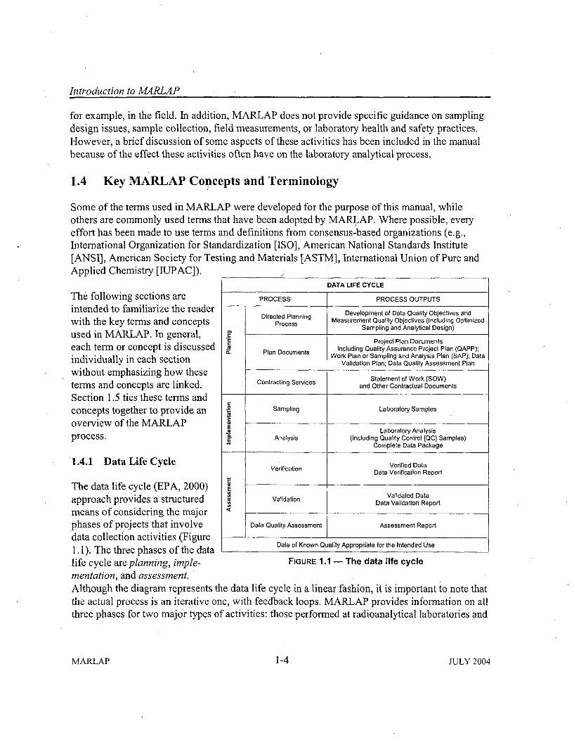
Introduction to MARLAP

for example, in the field. In addition, MARLAP does not provide specific guidance on samplingdesign issues, sample collection, field measurements, or laboratory health and safety practices.However, a brief discussion of some aspects of these activities has been included in the manualbecause of the effect these activities often have on the laboratory analytical process.

1.4 Key MARLAP Concepts and Terminology

Some of the terms used in MARLAP were developed for the purpose of this manual, whileothers are commonly used terms that have been adopted by MARLAP. Where possible, everyeffort has been made to use terms and definitions from consensus-based organizations (e.g.,International Organization for Standardization [ISO], American National Standards Institute[ANSI], American Society for Testing and Materials [ASTM], International Union of Pure andApplied Chemistry [IUPAC]).

F DATA LIFE CYCLE

The following sections areintended to familiarize the readerwith the key terms and conceptsused in MARLAP. In general,each term or concept is discussedindividually in each sectionwithout emphasizing how theseterms and concepts are linked.Section 1.5 ties these terms andconcepts together to provide anoverview of the MARLAPprocess.

1.4.1 Data Life Cycle

PROCESS PROCESS OUTPUTS

Directed Planning Development of Data Quality Objectives andProcess Measurement Quality Objectives (Including OptimizedPSampling and Analytical Design)

"r Project Plan DocumentsM Including Quality Assurance Project Plan (QAPP);

.Plan Documents Work Plan or Sampling and Analysis Plan (SAP); Data

Validation Plan; Data Quality Assessment Plan

gServices Statement of Work (SOW)

Contracting Sand Other Contractual Documents

0 Sampling Laboratory SamplesM

E Laboratory Analysis

E Analysis (Including Quality Control [QC] Samples)Complete Data Package

Verification Verified DataData Verification Report

EValidated Data

VData Validation Report

Data Quality Assessment Assessment Report

Data of Known Quality Appropriate for the Intended Use

The data life cycle (EPA, 2000)approach provides a structuredmeans of considering the majorphases of projects that involvedata collection activities (Figurel.1 . The three nhases of the data1' J. . . ... 1). T he..... .. .... ..... dat

life cycle are planning, imple- FIGURE 1.1 - The data life cyclementation, and assessment.Although the diagram represents the data life cycle in a linear fashion, it is important to note thatthe actual process is an iterative one, with feedback loops. MARLAP provides information on allthree phases for two major types of activities: those performed at radioanalytical laboratories and

MARLAP 1-4 JULY 2004

Introduction to MARLAP

those that direct, affect, or evaluate activities performed at radioanalytical laboratories (such asproject planning, development of plan documents, data verification and data validation).

One of MARLAP's specific objectives is to emphasize the importance of establishing the properlinkages among the three phases of the data life cycle. This results in an integrated and iterativeprocess that translates the expectations and requirements of data users into measurementperformance criteria for data suppliers. The integration of the three phases of the data life cycle iscritical to ensuring that the analytical data requirements (defined during the planning phase) canserve as measurement performance criteria during the implementation phase and subsequently asdata evaluation criteria during the assessment phase.

Without the proper linkages and integration of the three phases, there is a significant likelihoodthat the analytical data will not meet a project's data requirements. The data may be evaluatedusing criteria that have little relation to their intended use. Therefore, failure to integrate andadequately link the three phases of the data life cycle increases the likelihood of project costescalation or project failure.

1.4.2 Directed Planning Process

MARLAP recommends the use of a directed or systematic planning process. A directed planningprocess is an approach for setting well-defined, achievable objectives and developing a cost-effective, technically sound sampling and analysis design that balances the data user's tolerancefor uncertainty in the decision process with the resources available for obtaining data to support adecision. While MARLAP recommends and promotes the use of a directed planning process, itdoes not recommend or endorse any particular directed planning process. However, MARLAPemploys many of the terms and concepts associated with the data quality objective (DQO)process (ASTM D5792; EPA, 2000). This was done to ensure consistent terminology throughoutthe manual, and also because many of the terms and concepts of this process are familiar to thoseengaged in environmental data collection activities.

1.4.3 Performance-Based Approach

MARLAP provides the necessary guidance for using a performance-based approach to meet aproject's analytical data requirements. In a performance-based approach, the project-specificanalytical data requirements that are determined during directed planning serve as measurementperformance criteria for analytical selections and decisions. The project-specific analytical datarequirements also are used for the initial, ongoing, and final evaluation of the laboratory'sperformance and the laboratory's data. MARLAP provides guidance for using a performance-based approach for all three phases of the data life cycle for those projects that requireradioanalytical laboratory data. This involves not only using a performance-based approach forselecting an analytical protocol, but also using a performance-based approach for other project

JULY 2004 1-5 MARLAP

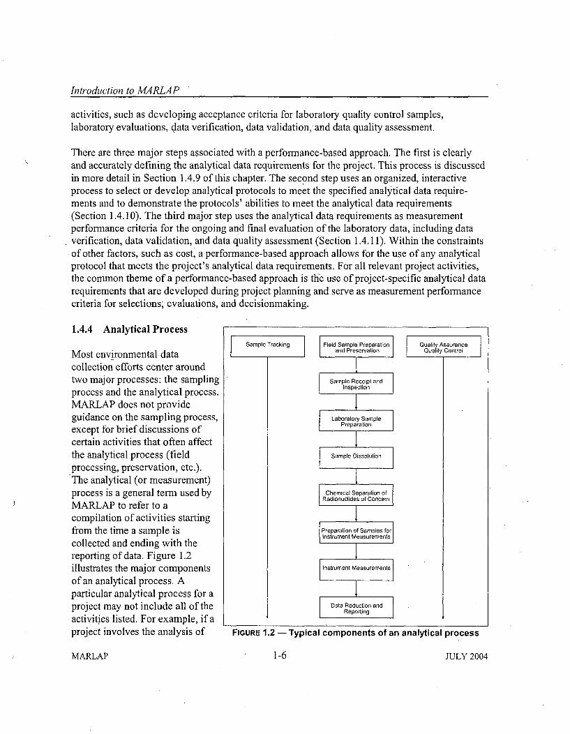
Introduction to MARLAP

activities, such as developing acceptance criteria for laboratory quality control samples,laboratory evaluations, data verification, data validation,and data quality assessment.

There are three major steps associated with a performance-based approach. The first is clearlyand accurately defining the analytical data requirements for the project. This process is discussedin more detail in Section 1.4.9 of this chapter. The second step uses an organized, interactiveprocess to select or develop analytical protocols to meet the specified analytical data require-ments and to demonstrate the protocols' abilities to meet the analytical data requirements(Section 1.4.10). The third major step uses the analytical data requirements as measurementperformance criteria for the ongoing and final evaluation of the laboratory data, including dataverification, data validation, and data quality assessment (Section 1.4.11). Within the constraintsof other factors, such as cost, a performance-based approach allows for the use of any analyticalprotocol that meets the project's analytical data requirements. For all relevant project activities,the common theme of a performance-based approach is the use of project-specific analytical datarequirements that are developed during project planning and serve as measurement performancecriteria for selections; evaluations, and decisionmaking.

1.4.4 Analytical Process

Most environmental datacollection efforts center aroundtwo major processes: the samplingprocess and the analytical process.MARLAP does not provideguidance on the sampling process,except for brief discussions ofcertain activities that often affectthe analytical process (fieldprocessing, preservation, etc.).The analytical (or measurement)process is a general term used byMARLAP to refer to acompilation of activities startingfrom the time a sample iscollected and ending with thereporting of data. Figure 1.2illustrates the major componentsof an analytical process. Aparticular analytical process for aproject may not include all of theactivities listed. For example, if aproject involves the analysis of

Sample Tracking S rField Sample Preparation Qand PreservationI

Sample Receipt andInspection

Laboratory SamplePreparation

Sample Dissolution

Chemical Separation ofRadionuclides of Concern

Preparation of Samples forInstrument MeasurementsIInatrument Measurements

Data Reduction andReporting

QualitQuay AssuranceIlly Control

FIGURE 1.2 -Typical components of an analytical process

MARLAP 1-6 JULY 2004

Introduction to MARLAP

tritium in drinking water, then the analytical process for the project will not include sampledissolution and the chemical separation of the radionuclide of concern. It is important to identifythe relevant activities of the analytical process for a particular project early in the planning phase.Once the activities have been identified, the analytical requirements of the activities can beestablished,'which will ultimately lead to defining how the activities will be accomplishedthrough the selection or development of written procedures.

1.4.5 Analytical Protocol

MARLAP uses the term "analytical protocol" to refer to a compilation of specific procedures andmethods that are performed in succession for a particular analytical process. For example, aprotocol for the analysis of drinking water samples for tritium would be comprised of the set ofprocedures that describe the relevant activities, such as sample tracking, quality control, fieldsample preparation and preservation, sample receipt and inspection, laboratory sample prepara-tion (if necessary), preparing the samples for counting, counting the samples, and data reductionand reporting. A written procedure may cover one or more of the activities, but it is unlikely thata single procedure will cover all of the activities of a given analytical process. With a perfor-mance-based approach, there may be a number of alternative protocols that might be appropriatefor a particular analytical process. Selecting or developing an analytical protocol requiresknowledge of the particular analytical process, as well as an understanding of the analytical datarequirements developed during the project planning phase.

1.4.6 Analytical Method

A major component of an analytical protocol is the analytical method, which normally includeswritten instructions for sample digestion, chemical separation (if required), and counting. It isrecognized that in many instances the analytical method may cover many of the activities of aparticular analytical process. Therefore attention is naturally focused on the selection ordevelopment of an analytical method. However, many analytical methods do not addressactivities such as field preparation and preservation, certain aspects of laboratory preparation,laboratory subsampling, etc., which are often important activities within an analytical process.The analytical protocol is generally more inclusive of the activities that make up the analyticalprocess than the analytical method.

1.4.7 Uncertainty and Error

An important aspect of sampling and measurement is uncertainty. The term "uncertainty" hasdifferent shades of meaning in different contexts, but generally the word refers to a lack ofcomplete knoowledge about something of interest. In the context of metrology (the science ofmeasurement), the more specific term "measurement uncertainty" often will be used. "Uncertain-ty (of measurement)" is defined in the Guide to the Expression of Uncertainty in Measurement(ISO 1995-"GUM") as a "parameter, associated with the result of a measurement, that charac-

JULY 2004 1-7 MARLAP

Introduction to MARLAP

terizes the dispersion of values that could reasonably be attributed to the measurand." The"measurand" is the quantity being measured. MARLAP recommends the terminology andmethods of GUM for describing, evaluating, and reporting measurement uncertainty. Theuncertainty of a measured value is typically expressed as an estimated standard deviation, calleda "standard uncertainty" (or "one-sigma uncertainty"). The standard uncertainty of a calculatedresult usually is obtained by propagating the standard uncertainties of a number of othermeasured values, and in this case, the standard uncertainty is called a "combined standarduncertainty." The combined standard uncertainty may be multiplied by a specified factor called a"coverage factor" (e.g., 2 or 3) to obtain an "expanded uncertainty" (a "two-sigma" or "three-sigma" uncertainty), which describes an interval about the result that can be expected to containthe true value with a specified high probability. MARLAP recommends that either the combinedstandard uncertainty or an expanded uncertainty be reported with every result. Chapter 19discusses the terminology, notation, and methods of GUM in more detail and provides guidancefor applying the concepts to radioanalytical measurements.

While measurement uncertainty is a parameter associated with an individual result and iscalculated after a measurement is performed, MARLAP uses the term "method uncertainty" torefer to the predicted uncertainty of a measured value that likely would result from the analysis ofa sample at a specified analyte concentration. Method uncertainty is a method performancecharacteristic much like the detection capability of a method. Reasonable values for bothcharacteristics can be predicted for a particular method based on typical values for certainparameters and on information and assumptions about the samples to be analyzed. Thesepredicted values can be used in the method selection process to identify the most appropriatemethod based on a project's data requirements. Chapter 3 provides MARLAP's recommenda-tions for deriving analytical protocol selection criteria based on the required method uncertaintyand other analytical requirements.

When a decisionmaker bases a decision on the results of measurements, the measurementuncertainties affect the probability of making a wrong decision. When sampling is involved,sampling statistics also contribute to the probability of a wrong decision. Because decision errorsare possible, there is uncertainty in the decisionmaking process. MARLAP uses the terms"decision uncertainty" or "uncertainty of the decision" to refer to this type of uncertainty.Decision uncertainty is usually expressed as the estimated probability of a decision error underspecified assumptions. Appendix B discusses decision uncertainty further in the context of theDQO process.

A concept that should not be confused with uncertainty is error. In general, error refers tosomething that deviates from what is correct, right or true. In terms of measurements such aslaboratory analyses, the difference between the measured result and the actual valuc of themeasurand is the error of the measurement. Because the actual value of the measurand isgenerally not known, the measurement error cannot be determined. Therefore, the error of ameasurement is primarily a theoretical concept with little practical use. However, the

MARLAP 1-8 JULY 2004

Introduction to MARLAP,

measurement uncertainty, which provides an estimated bound for the likely size of themeasurement error, is very useful and plays a-key role in MARLAP's performance-basedapproach.

1.4.8 Precision, Bias, and Accuracy

Analytical data requirements often have been described interms of precision and bias. Precisionis usually expressed as a standard deviation, which measures the dispersion of measured valuesabout their mean. It is sometimes more natural to speak of "imprecision," because larger valuesof the standard deviation indicate less precision. MARLAP considers bias to be a persistentdifference between the measured result and the true value of the quantity being measured, whichdoes not vary if the measurement is repeated. If the measurement process is in statistical control,then precision may be improved by averaging the results of many independent measurements ofthe same quantity. Bias is unaffected by averaging (see Section 6.5.5.7).

A bias in a data set may be caused by measurement errors that occur in steps of the measurementprocess that are not repeated, such as the determination of a half-life. Imprecision may be causedby measurement errors in steps that are repeated many times, such as weighing, pipetting, andradiation counting. However, distinguishing between bias and precision is complicated by thefact that some steps in the process, such as instrument calibration or tracer preparation, arerepeated at frequencies less than those of other steps, and the measurement errors in seldomrepeated steps may affect large blocks of data. Consequently, measurement errors that produceapparent biases in small data sets might adversely affect precision in larger data sets.

Because the same type of measurement error may produce either bias or precision, depending onone's point of view, the concept of measurement uncertainty, described in Section 1.4.7, treats alltypes of measurement error alike and combines estimates of their magnitudes into a singlenumerical parameter (i.e., combined standard uncertainty). The concepts of precision and bias areuseful in context when a measurement process or a data set consisting of many measurementresults is considered. When one considers only a single measurement result, the concept ofmeasurement uncertainty tends to be more useful than the concepts of precision and bias.Therefore, it is probably best to consider precision and bias to be characteristics of themeasurement process or of the data set, and to consider measurement uncertainty to be an aspectof each individual result.

Quality control samples are analyzed for the purpose of assessing precision and bias. Spikedsamples and method blanks are typically used to assess bias, and duplicates are used to assessprecision. Because a single measurement of a spike or blank cannot in principle distinguishbetween precision and bias, a reliable estimate of bias requires a data set that includes many suchmeasurements.

JULY 2004 1-9 MARLAP

Introduction to MARLAP

Different authors have given the word accuracy different technical definitions, expressed interms of bias and precision. MARLAP avoids all of these technical definitions and uses the term"accuracy" in its common, ordinary sense, which is consistent with its definition in theInternational Vocabulary of Basic and General Terms in Metrology (ISO, 1993). In MARLAP'sterminology, the result of a measurement is "accurate" if it is close to the true value of thequantity being measured. Inaccurate results may be caused either by bias or precision in themeasurement process.

While it is recognized that the terms bias, precision, and accuracy are commonly used in datacollection activities, these terms are used somewhat sparingly in this manual. MARLAPemphasizes and provides guidance in the use of measurement uncertainty as a means ofestablishing analytical data requirements and in the evaluation of single measurement results.

1.4.9 Performance Objectives: Data Quality Objectives and Measurement QualityObjectives

One of the outputs of a directed planning process is DQOs for a project or program. DQOs arequalitative and quantitative statements that clarify the study objectives, define the mostappropriate type of data to collect, determine the most appropriate conditions from which tocollect the data, and specify tolerable limits on decision error rates (ASTM D5792; EPA, 2000).DQOs apply to all data collection activities associated with a project or program, includingsampling and analysis. In particular, DQOs should encompass the "total uncertainty" resultingfrom all data collection activities, including analytical and sampling activities.

From an analytical perspective, a process of developing the analytical data requirements from theDQOs of a project is essential. These analytical data requirements serve as measurement perfor-mance criteria or objectives of the analytical process. MARLAP refers to these performanceobjectives as "measurement quality objectives" (MQOs). The MARLAP Manual providesguidance on developing the MQOs from the overall project DQOs (Chapter 3). MQOs can beviewed as the analytical portion of the DQOs and are therefore project-specific. MARLAPprovides guidance on developing MQOs during project planning for select method performancecharacteristics, such as method uncertainty at a specified concentration; detection capability;quantification capability; specificity, or the capability of the method to measure the analyte ofconcern in the presence of interferences; range; ruggedness, etc. An MQO is a statement of aperformance objective or requirement for a particular method performance characteristic. LikeDQOs, MQOs can be quantitative and qualitative statements. An example of a quantitative MQOwould be a statement of a required method uncertainty at a specified radionuclide concentration,such as the action level-i.e., "a method uncertainty of 3.7 Bq/kg (0.10 pCi/g) or less is requiredat the action 'Level of 37 Bqkg (1.0 pi, /g)." An example of a qualitative MLQO would be astatement of the required specificity of the analytical protocol-the ability to analyze for theradionuclide of concern given the presence of interferences-i.e., "the protocol must be able toquantify the amount of 226Ra present given high levels of 23̀U in the samples."

MARLAP 1-10 JULY 2004

Introduction to MARLAP

The MQOs serve as measurement performance criteria for the selection or development ofanalytical protocols and for the initial evaluation of the analytical protocols. Once the analyticalprotocols have been selected and evaluated, the MQOs serve as criteria for the ongoing and finalevaluation of the laboratory data, including data verification, data validation, and data qualityassessment. In a performance-based approach, analytical protocols are either selected or rejectedfor a particular project, to a large measure, based on their ability or inability to achieve the statedMQOs. Once selected, the performance of the analytical protocols is evaluated using the project-specific MQOs.

1.4.10 Analytical Protocol Specifications

MARLAP uses the term "analytical protocol specifications" (APSs) to refer to the output of adirected planning process that contains the project's analytical data requirements in an organized,concise form. In general, there will be an APS developed for each analysis type. Thesespecifications serve as the basis for the evaluation and selection of the analytical protocols thatwill be used for a particular project. In accordance with a performance-based approach, the APSscontain only the minimum level of specificity required to meet the project's analytical datarequirements without dictating exactly how the requirements are to be met. At a minimum, theAPSs should indicate the analyte of interest, the matrix of concern, the type and frequency ofquality control (QC) samples, and provide the required MQOs and any specific analytical processrequirements, such as chain-of-custody for sample tracking. In most instances, a particular APSdocument would be a one-page form (see Chapter 3, Figure 3.2). Depending on the particularproject, a number of specific analytical process requirements may be included. For example, ifproject or process knowledge indicates that the radionuclide of interest exists in a refractoryform, then the APSs may require a fusion step for sample digestion.

Within the constraints of other factors, such as cost, MARLAP's performance-based approachallows the use of any analytical protocol that meets the requirements in the APSs. The APSs-inparticular the MQOs-are used to select and evaluate the analytical protocols. Once theanalytical protocols have been selected and evaluated, the APSs then serve as criteria for theongoing and final evaluation of the laboratory data, including data verification, data validation,and data quality assessment.

1.4.11 The Assessment Phase

The MARLAP Manual provides guidance for the assessment phases for those projects thatrequire the laboratory analysis of radionuclides. The guidance on the assessment phase ofprojects focuses on three major activities: data verification, data validation, and data qualityassessment.

Data verification assures that laboratory conditions and operations were compliant with thestatement of work and any appropriate project plan documents (e.g., Quality Assurance Project

JULY 2004 1-11 MARLAP

Introduction to MARLAP

Plan), which may reference laboratory documents such as laboratory standard operatingprocedures. Verification compares the material delivered by the laboratory to these requirements(compliance) and checks for consistency and comparability of the data throughout the datapackage, correctness of calculations, and completeness of the results to ensure that all necessary

documentation is available. The verification process usually produces a report identifying whichrequirements are not met. The verification report may be used to determine payment forlaboratory services and to identify problems that should be investigated during data validation.Verification works iteratively and interactively with the generator (i.e., laboratory) to assurereceipt of all available, necessary data. Although the verification process identifies specificproblems, the primary function should be to apply appropriate feedback resulting in correctiveaction improving the analytical services before the work is completed.

Validation addresses the reliability of the data. The validation process begins with a review of theverification report and laboratory data package to screen the areas of strength and weakness ofthe data set. The validator evaluates the data to determine the presence or absence of an analyteand the uncertainty of the measurement process for contaminants of concern. During validation,the technical reliability and the degree of confidence in reported analytical data are considered.Validation "flags" (i.e., qualifiers) are applied to data that do not meet the acceptance criteriaestablished to assure data meet the needs of the project. The product of the validation process is avalidation report noting all data sufficiently inconsistent with the validation acceptance criteria inthe expert opinion of the validator. The appropriate data validation tests should be establishedduring the project planning phase.

Data quality assessment (DQA), the third and final step of the assessment phase, is defined as the"scientific and statistical evaluation of data to determine if data are of the right type, quality, andquantity to support their intended use." DQA is more global in its purview than the previousverification and validation steps. DQA, in addition to reviewing the issues raised during verifica-tion and validation, may be the first opportunity to review other issues, such as field activitiesand their impact on data quality and usability. DQA should consider the combined impact of allproject activities in making a data usability determination, which is documented in a DQA report.

1.5 The MARLAP Process

An overarching objective of the MARLAP Manual is to provide a framework and informationfor the selection, development, and evaluation of analytical protocols and the resulting laboratorydata. The MARLAP process is a performance-based approach that develops APSs and uses theserequirements as criteria for the analytical protocol selection, development and evaluationprocesses, and for the evaluation of the resulting laboratory data. This process, which spans thethree phases of the data life cycle for a project-planning, implementation and assessment-isthe basis for achieving MARLAP's basic goal of ensuring that radioanalytical data will meet a

MARLAP 1-12 JULY 2004

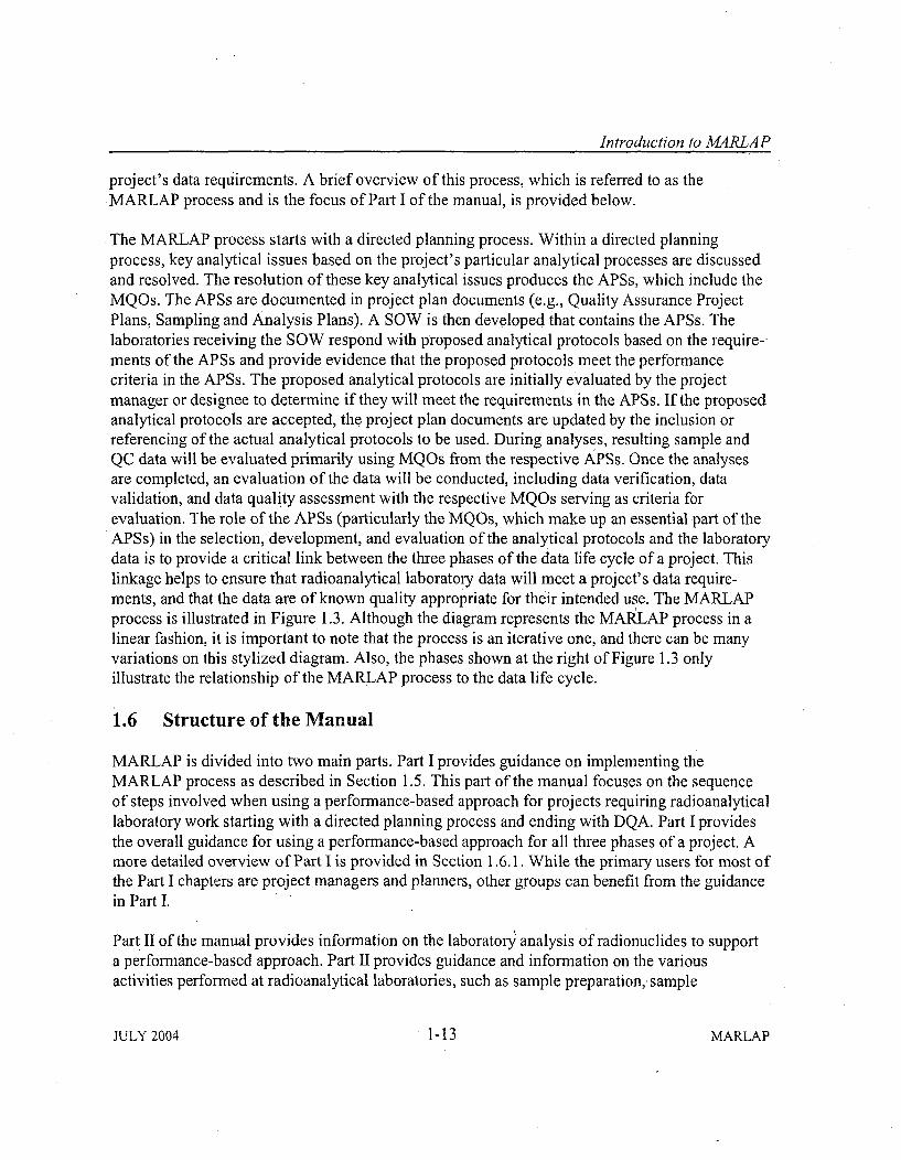
Introduction to MARLAP

project's data requirements. A brief overview of this process, which is referred to as the•MARLAP process and is the focus of Part I of the manual, is provided below.

The MARLAP process starts with a directed planning process. Within a directed planningprocess, key analytical issues based on the project's particular analytical processes are discussedand resolved. The resolution of these key analytical issues produces the APSs, which include theMQOs. The APSs are documented in project plan documents (e.g., Quality Assurance ProjectPlans, Sampling and Analysis Plans). A SOW is then developed that contains the APSs. Thelaboratories receiving the SOW respond with proposed analytical protocols based on the require-ments of the APSs and provide evidence that the proposed protocols meet the performancecriteria in the APSs. The proposed analytical protocols are initially evaluated by the projectmanager or designee to determine if they will meet the requirements in the APSs. If the proposedanalytical protocols are accepted, the project plan documents are updated by the inclusion orreferencing of the actual analytical protocols to be used. During analyses, resulting sample andQC data will be evaluated primarily using MQOs from the respective APSs. Once the analysesare completed, an evaluation of the data will be conducted, including data verification, datavalidation, and data quality assessment with the respective MQOs serving as criteria forevaluation. The role of the APSs (particularly the MQOs, which make up an essential part of theAPSs) in the selection, development, and evaluation of the analytical protocols and the laboratorydata is to provide a critical link between the three phases of the data life cycle of a project. Thislinkage helps to ensure that radioanalytical laboratory data will meet a project's data require-ments, and that the data are of known quality appropriate for their intended use. The MARLAPprocess is illustrated in Figure 1.3. Although the diagram represents the MARLAP process in alinear fashion, it is important to note that the process is an iterative one, and there can be manyvariations on this stylized diagram. Also, the phases shown at the right of Figure 1.3 onlyillustrate the relationship of the MARLAP process to the data life cycle.

1.6 Structure of the Manual

MARLAP is divided into two main parts. Part I provides guidance on implementing theMARLAP process as described in Section 1.5. This part of the manual focuses on the sequenceof steps involved when using a performance-based approach for projects requiring radioanalyticallaboratory work starting with a directed planning process and ending with DQA. Part I providesthe overall guidance for using a performance-based approach for all three phases of a project. Amore detailed overview of Part I is provided in Section 1.6.1. While the primary users for most ofthe Part I chapters are project managers and planners, other groups can benefit from the guidancein Part I.

Part II of the manual provides information on the laboratory analysis of radionuclides to supporta performance-based approach. Part II provides guidance and information on the variousactivities performed at radioanalytical laboratories, such as sample preparation,. sample

JULY 2004 1-13 MARLAP

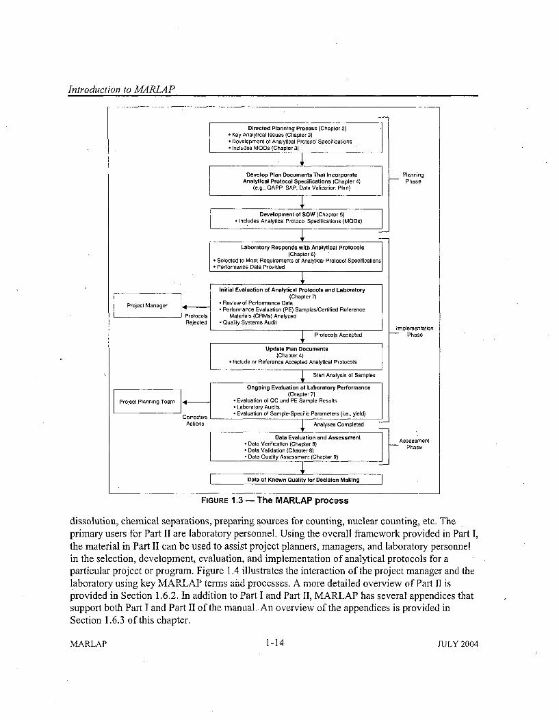
Introduction to MARLAP

Directed Planning Process (Chapter 2)* Key Analytical Issues (Chapter 3)* Development of Analytical Protocol Specifications* Includes MOOs (Chapter 3)

Develop Plan Documents That IncorporateAnalytical Protocol Specifications (Chapter 4)

(e.g., QAPP, SAP, Data Validation Plan)

Development of SOW (Chapter 5) I

Includes Analytical Protocol Specifications (MQOs)

Planning- Phase

Laboratory Responds with Analytical Protocols(Chapter

6)

* Selected to Meet Requirements of Analytical Protocol Specifications* Performance Data Provided

Project Manager 4

ProtocolsRejected

Project Planning Team .

CorrectiveActions

Initial Evaluation of Analytical Protocols and Laboratory(Chapter 7)

* Review of Performance Data* Performance Evaluation (PE) Samples/Certified Reference

Materials (CRMs) Analyzed* Quality Systems Audit

I

, Protocols Accepted

Update Plan Documents(Chapter 4)

Include or Reference Accepted Analytical Protocols

Start Analysis of Samples

Ongoing Evaluation of Laboratory Performance(Chapter 7)

* Evaluation of OC and PE Sample Results* Laboratory Audits* Evaluation of Sample-Specific Parameters (i.e., yield)

ImplementationPhase

AssessmentPhase

Analyses Completed

Data Evaluation and Assessment* Data Verification (Chapter 8)

Data Validation (Chapter 8)* Data Quality Assessment (Chapter 9)

Data of Known Quality for Decision Making

FIGURE 1.3 - The MARLAP process

dissolution, chemical separations, preparing sources for counting, nuclear counting, etc. Theprimary users for Part II are laboratory personnel. Using the overall framework provided in Part I,the material in Part II can be used to assist project planners, managers, and laboratory personnelin the selection, development, evaluation, and implementation of analytical protocols for aparticular project or program. Figure 1.4 illustrates the interaction of the project manager and thelaboratory using key MA LAP terms ard proccsses. A more detailed overview of Part 11 isprovided in Section 1.6.2. In addition to Part I and Part II, MARLAP has several appendices thatsupport both Part I and Part HI of the manual. An overview of the appendices is provided inSection 1.6.3 of this chapter.

MARLAP 1-14 JULY 2004

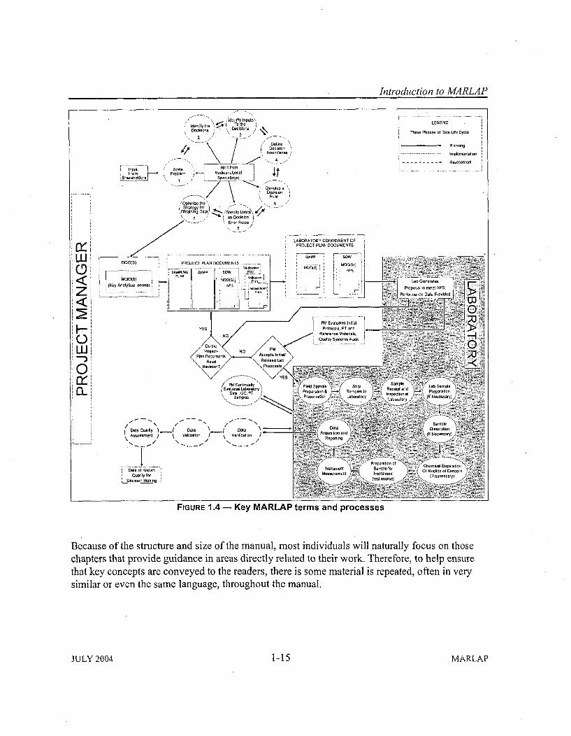
Introduction to AMARLAP

Id e n tify \th : 'ld e n t • In p u ts '; dent fy fhe • To thoSDecisions De ' LcisiOns /,

Boundaries

Is Input from Ien R•d.odo.oo.a-IyfiW

enelop a

OntionleRufe

. n~ the 5 _ S caits _ " ... "

LEGEND

mThree Phaes of Data Life Cycle

i Planning

... ..................... Implemo ntation

-Assessmnent

Inp iput t.L Fro ' PFobLShareheiders -\

Strafegn for fipeofy L.. .. n ", o "iObtainlng Dat a,' Specify Liatas,'\ 7 ,'of n on isloe i

Erro Rale.

Uj:

0z

0w,03

LABORATORY COMPONENT OF

PROJECT PLAN DOCUMENTS

QAPP Wgop . ........

i cstol I r ""i

FIGURE 1.4 - Key MARLAP terms and processes

Because of the structure and size of the manual, most individuals will naturally focus on thosechapters that provide guidance in areas directly related to their work. Therefore, to help ensurethat key concepts are conveyed to the readers, there is some material is repeated, often in verysimilar or even the same language, throughout the manual.

JULY 2004 1-15 MARLAP

Introduction to MA4RLAP

1.6.1 Overview of Part I

Figure 1.3, the MARLAP Process on page 1-14, illustrates the sequence of steps that make up aperformance-based approach for the planning, implementation, and assessment phases ofradioanalytical projects. The remainder of Part I closely tracks this sequence:

" Chapter 2, Project Planning Process, provides an overview of the directed planning processand its outputs.

" Chapter 3, Key Analytical Planning Issues and Developing Analytical Protocol Specifica-tions, describes key analytical planning issues that need to be addressed during a directedplanning process and provides guidance on developing APSs, which are outputs of theplanning process.

" Chapter 4, Project Plan Documents, provides guidance on the linkage between projectplanning and project plan documents, with an overview of different types of project plandocuments (e.g., work plans, quality assuranceproject plans, sampling and analysis plans).

" Chapter 5, Obtaining Laboratory Services, provides guidance on developing a statement ofwork that incorporates the APSs.

" Chapter 6, Selection and Application of an Analytical Method, provides guidance on selectingor developing analytical protocols that will meet the MQOs and other requirements asoutlined in the APSs. Unlike the rest of Part I, this chapter is intended primarily for labora-tory personnel, because under a performance-based approach, a laboratory may use anyprotocol that meets therequirements of the APSs. (Other factors, such as cost, also willinfluence the selection of analytical protocols.)

" Chapter 7, Evaluating Methods and Laboratories, provides guidance on the initial andongoing evaluation of analytical protocols and also provides guidance on the overallevaluation of radioanalytical laboratories.

" Chapter 8, Radiochemical Data Verification and Validation, provides an overviewv of the dataevaluation process, provides general guidelines for data verification and validation, andprovides "tools" for data validation.

" The last chapter of Part I, Chapter 9, Data Quality Assessment, discusses data qualityassessment and provides guidance on linking data quality assessment to the planning process.

MARLAP 1-16 JULY 2004

Introduction to MARLAP

1.6.2 Overview of Part II

The chapters in Part II are intended to provide information on the laboratory analysis ofradionuclides. The chapters provide information on many of the options available for analyticalprotocols, and discuss common advantages and disadvantages of each. The chapters highlightcommon analytical problems and ways to identify and correct them. The chapters also serve toeducate the reader by providing a detailed explanation of the typical activities performed at aradioanalytical laboratory. Consistent with a performance-based approach, the chapters in Part IIdo not contain detailed step-by-step instructions on how to perform certain laboratory tasks, suchas the digestion of a soil sample. The chapters do contain information and guidance intended toassist primarily laboratory personnel in deciding on the best approach for a particular laboratorytask. For example, while the chapter on sample dissolution does not contain step-by-stepinstructions on how to dissolve a soil sample, it does provide information on acid digestion,fusion techniques, and microwave digestion, which is intended to help the reader select the mostappropriate technique or approach for a particular project.

The primary audience for Part II is laboratory personnel and the chapters generally contain asignificant amount of technical information. While the primary target audience is laboratorypersonnel, other groups, such as project planners and managers, can benefit from the guidance inPart II. Listed below are the chapters that make up Part II of the manual. It should be noted thatPart II of the manual does not provide specific guidance for some laboratory activities that arecommon to all laboratories, such as laboratory quality assurance, and laboratory health and safetypractices. This is primarily due to the fact that these activities are not unique to radioanalyticallaboratories and considerable guidance in these areas already exists.

Chapter 10'Chapter IlChapter 12Chapter 13Chapter 14Chapter 15Chapter 16

Chapter 17Chapter 18Chapter 19Chapter 20

Field and Sampling Issues That Affect Laboratory MeasurementsSample Receipt, Inspection, and TrackingLaboratory Sample PreparationSample DissolutionSeparation TechniquesQuantification of RadionuclidesData Acquisition, Reduction, and Reporting for Nuclear CountingInstrumentationWaste Management in a Radioanalytical LaboratoryLaboratory Quality ControlMeasurement UncertaintyDetection and Quantification Capabilities

Chapters 10 through 16 provide information on the typical components of an analytical processin the order in which activities that make up an analytical process are normally performed. Whilenot providing step-by-step procedures for activities such as sample preservation, sampledigestion, nuclear counting, etc., the chapters do provide an overview of options available for the

JULY 2004 1-17 MARLAP

Introduction to MARLAP

various activities and importantly, provide information on the appropriateness of the assortedoptions under a variety of conditions.

Chapter 17, Waste Management in a Radioanalytical Laboratory, provides an overview of manyof the regulations for waste disposal and provides guidance for managing wastes in a radioana-lytical laboratory. Chapter 18, Laboratory Quality Control, provides guidance on monitoring keylaboratory performance indicators as a means of determining if a laboratory's measurementprocesses are in control. The chapter also provides information on likely causes of excursions forselected laboratory performance indicators, such as chemical yield, instrument background,quality control samples, etc.

Chapters 19, Measurement Uncertainty, and 20, Detection and Quantification Capabilities,provide information on statistical principles and methods applicable to radioanalytical measure-ments, calibrations, data interpretation, and quality control. Topics covered in the chapter includedetection and quantification, measurement uncertainty, and procedures for estimatinguncertainty.

1.6.3 Overview of the Appendices

Seven appendices provide additional details on specific topics discussed in Part I and Part IIchapters. Appendices A through E primarily support Part I chapters (project planning issues) andAppendices F and G primarily support the chapters in Part II (laboratory implementation issues).

" Appendix A, Directed Planning Approaches, provides an overview of a number of directedplanning processes and discusses some common elements of the different approaches.

" Appendix B, The Data Quality Objective Process, provides an expanded discussion of theData Quality Objectives Process including detailed guidance on setting up a "gray region"and establishing tolerable decision error rates.

" Appendix C, Measurement Quality Objectives for Method Uncertainty and Detection andQuantification Capability, provides the rationale and guidance for developing MQOs forselect method performance characteristics.

" Appendix D, Content of Project Plan Documents, provides guidance on the appropriatecontent of plan documents.

" Appendix E, Contracting Laboratory Services, contains detailed guidance on contractinglaboratory services.

" Appendix F, Laboratory Subsampling, provides information on improving and evaluatinglaboratory subsampling techniques,

MARLAP 1-18 JULY 2004

Introduction to MARLAP

• Appendix G, Statistical Tables, provides a compilation of statistical tables.

1.7 References

American Society for Testing and Materials (ASTM) D5792. Standard Practice for Generationof Environmental Data Related to Waste Management Activities. Development of DataQuality Objectives, 1995.

International Organization for Standardization (ISO). 1993. International Vocabulary of Basicand General Terms in Metrology. ISO, Geneva, Switzerland.

International Organization for Standardization (ISO). 1995. Guide to the Expression ofUncertainty in Measurement. ISO, Geneva, Switzerland.

MARSSIM. 2000. Multi-Agency Radiation Survey and Site Investigation Manual, Revision L.NUREG-1575 Rev 1, EPA 402-R-97-016 Revl, DOE/EH-0624 Revl. August. Available atwww.epa.gov/radiation/marssim/.

U.S. Environmental Protection Agency (EPA). 2000. Guidance for the Data Quality ObjectiveProcess (EPA QA/G-4). EPA/600/R-96/055, Washington, DC. Available at www.epa.gov/quality 1/qadocs.html.

JULY 2004 1-19 MARLAP

18 LABORATORY QUALITY CONTROL

18.1 Introduction

This chapter addresses internal laboratory quality control (QC), the purpose of which is tomonitor performance, identify problems, and initiate corrective action. If project requirements aremore stringent than typical laboratory QC criteria, the project manager and the laboratory shouldconfer to see whether the laboratory can accommodate the project QC requirements. Project QCrequirements are addressed in Part I of MARLAP.

Laboratory data should be produced under a quality system' that incorporates planning,implementing, and internal assessment of the work performed by the laboratory, including QC.MARLAP fully endorses the need for a laboratory quality system and a quality manual thatdelineates the quality assurance (QA) policies and QC practices of the laboratory. A laboratory'squality system should ensure that laboratory processes and measurements are "in statisticalcontrol," which means that the distribution of measured results is stable.

This chapter's purpose is to provide guidance to laboratory staff on those activities and profes-sional practices a radioanalytical laboratory should undertake to produce data of known quality.This chapter also ,shows how to use statistical techniques to monitor specific measures of theanalytical process to indicate the level of control of the analytical process within the laboratory.These measures are called "performance indicators," and the statistical techniques involve theuse of control charts. Monitoring performance indicators through control charts enables theidentification of trends. The laboratory can then address analytical problems and help improvethe analytical process. Section 18.3.2 and Attachment 18A at the end of this chapter provideexamples of several types of charts. The use ofstatistical techniques is the preferred method for Contents

implementing quality control in the laboratory 18.1 Introduction ...................... 18-1(Attachment 18B). The chapter also identifies 18.2 Quality Control ..................... 18-3

specific performance indicators, the principles 18.3 Evaluation of Performance Indicators ..... 18-3

that govern their use, indications and under- 18.4 Radiochemistry Performance Indicators ... 18-9

lying causes of excursions, statistical means of 18.5 Instrumentation Performance Indicators . . 18-24

evaluating performance indicators, and 18.6 Related Concerns .................... 18-5418.7 References ......................... 18-65

examples of root-cause evaluations. Attachment 18A: Control Charts ............. 18-69

Attachment 18B: Statistical Tests for QC Results 18-81

'A quality system is a structured and documented management framework that describes the policies, objectives,principles, organizational authority, responsibilities, accountability, and implementation plan of an organization forensuring quality in its work processes, products (items), and services. The quality system provides for planning,implementing, and assessing the work performed by the organization and for carrying out required quality assuranceand quality control (ANSI/ASQC E4, 1994). General requirements for testing laboratories can be found in ISO/IEC17025.

JULY 2004 18-1 MARLAP

Laboratory Quality Control

This chapter addresses the control of the analytical process in the laboratory, as distinct frommeeting the typical analytical needs of a specific project. Quality control provides quantitativeestimates of analysis and measurement controls that can be used to determine compliance withproject objectives.

18.1.1 Organization of Chapter

Chapter 18 has five major sections in addition to this introduction. Section 18.2 provides ageneral overview of QC and its application in the laboratory setting. Section 18.3 discusses theimportance of evaluating performance indicators and provides statistical means for their evalua-tion. Sections 18.4 and 18.5 identify primary radiochemistry and instrumentation performanceindicators, respectively, and discuss each in detail. Section 18.6 discusses other aspects of theanalytical process that require scrutiny but are not formally considered performance indicators.

18.1.2 Format

The chapter is presented in a different format than the preceding chapters in order to highlight theperformance indicators and to give examples. For each performance indicator, general guidanceis provided in the format shown below.

Issue: Defines and summarizes the performance indicator

Discussion: Identifies those matters important to the performance indicator, including:

" What is the performance indicator and how does it work?

" Why is the performance indicator important, and what is its impact on the quality of themeasurement?

" What is the relationship of the performance indicator and the combined standard uncertaintyderived for the analytical method?

" What are the acceptable limits of the performance indicator?

" What are the key assumptions underlying the performance indicator?

* What limits and cautions are associated with the assumptions made?

" How sensitive is the quality of the measurement to the assumptions made?

• What is the appropriate frequency for assessing this performance indicator?

MARLAP 18-2 JULY 2004

Laboratory Quality Control

Excursions: "Excursions" are departures from the expected condition. This section addresses thelikely types of excursions encountered during laboratory analysis and explains what each mayindicate. This section also discusses the potential reasons for these excursions and theimplications for the analytical results.

Examples: Where appropriate, this section provides typical examples of excursions, potentialreasons for excursions, and additional information.

18.2 Quality Control

Quality control includes all technical activities that measure the attributes and performance of aprocess, item, or service against defined standards to verify that they meet the stated require-ments established by the customer. It also includes operational techniques and activities that areused to fulfill requirements for quality (ANSI/ASQC E4, 1994).

QC may not always detect blunders. Good laboratory practices, in addition to adherence tostandard operating procedures (SOPs), are part of the overall QA/QC aspects needed to check thelaboratory's performance. To monitor and control quality, laboratories use performance indica-tors, which are instrument- or protocol-related parameters that are routinely monitored to assessthe laboratory's estimate of measurement uncertainty, precision, bias, etc. Initially, these para-meters are used to maintain or demonstrate control over the analytical process. The performanceindicators should be tracked by appropriate personnel. If the performance indicator control limitsare exceeded, management should be informed and corrective action should be initiated.

Figure 18.1 lists some of the potential causes for radioanalytical control excursions. By no meansis the list complete, and the reader should be aware of additional potential causes of excursionsthat are presented in the rest of this chapter and the other chapters. Many problems are complexand have multiple components that could complicate the search for causes of protocol or instru-ment related excursions.'A metrologist or radiochemist should be consulted to identify andremedy any analytical problems.

18.3 Evaluation of Performance Indicators

18.3.1 Importance of Evaluating Performance Indicators

As stated previously, performance indicators are measures of the analytical process that thelaboratory monitors as part of its routine QC program. Performance indicators demonstratewhether the analytical process is performing as planned, when it has exhibited a statisticalanomaly that requires investigation, and when a system has failed. Accordingly, monitoringperformance indicators using established statistical techniques provides the laboratory with aneffective tool for self assessment that allows the identification of trends or conditions that, whilestill within the established bounds of acceptability, are drifting or trending out of control. Theseconditions can be addressed prospectively, allowing the laboratory to maintain analytical control.

JULY 2004 18-3 MARLAP

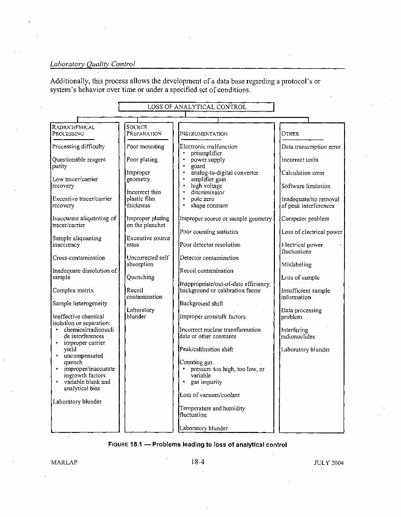
Laboratory Quality Control

Additionally, this process allows the development of a data base regarding a protocol's orsystem's behavior over time or under a specified set of conditions.

LOSS OF ANALYTICAL CONTROLI _

IRADIOCHEMICAL

PROCESSING

Processing difficulty

Questionable reagentpurity

Low tracer/carrierrecovery

Excessive tracer/carrierrecovery

Inaccurate aliquanting oftracer/carrier

Sample aliquantinginaccuracy

Cross-contamination

Inadequate dissolution ofsample

Complex matrix

Sample heterogeneity

Ineffective chemicalisolation or separation:

" chemical/radionuclide interferences

" improper carrieryield

* uncompensatedquenchimproper/inaccurateingrowth factors

* variable blank andanalytical bias

Laboratory blunder

ISOURCE

PREPARATION

Poor mounting

Poor plating

Impropergeometry

Incorrect thinplastic filmthickness

Improper platingon the planchet

Excessive sourcemass

Uncorrected self

absorption

Quenching

Recoilcontamination

Laboratoryblunder

INSTRUMENTATION

Electronic malfunction* preamplifier* power supply* guard* analog-to-digital convertor* amplifier gain* high voltage* discriminator* pole zero* shape constant

Improper source or sample geometry

Poor counting statistics

Poor detector resolution

Detector contamination

Recoil contamination

Inappropriate/out-of-date efficiency,background or calibration factor

Background shift

Improper crosstalk factors

Incorrect nuclear transformationdata or other constants

Peak/calibration shift

Counting gas" pressure too high, too low, or

variable" gas impurity

Loss of vacuum/coolant

Temperature and humidityfluctuation

Laboratory blunder

OTHER

Data transcription error

Incorrect units

Calculation error

Software limitation

Inadequate/no removalof peak interferences

Computer problem

Loss of electrical power

Electrical powerfluctuations

Mislabeling

Loss of sample

Insufficient sampleinformation

Data processingproblem

Interferingradionuclides

Laboratory blunder

FIGURE 18.1 - Problems leading to loss of analytical control

MARLAP 18-4 JULY 2004

Laboratory Quality Control

18.3.2 Statistical Means of Evaluating Performance Indicators - Control Charts

The primary tool for statistical quality control is the control chart (see Attachment 18A). Thetheory that underlies a control chart is statistical hypothesis testing (see NIST/SEMA TECH e-Handbook of Statistical Methods, http://www.itl.nist.gov/div898/handbook/, 2003). Theimplementation of a control chart makes the theory transparent to the average user and reducesthe process of statistical inference to answering simple questions, such as, "Is the measuredparameter greater than the upper control limit?" or "Is the measured parameter in the warningregion?"

In theory, to test whether a parameter 0 is above or below a certain value 00, a test statistic isdefined and its distribution is determined under the assumption that 0 = 00 (the null hypothesis).The value of the statistic is calculated and compared to critical values to test the assumption. Inpractice, a control chart is designed so that a non-statistician can perform these tests easily bycomparing the measured value of the parameter to control limits and warning limits.

Most control charts do not implement hypothesis tests in a rigorous manner that allows decisionerror rates to be precisely determined. The charts are intended to be simple and practical tools foruse even in situations where the assumptions needed for a rigorous test are not verifiable.

Every control chart has control limits, which define the acceptable range of the monitoredvariable. Many charts have both upper and lower limits. However, when changes in only onedirection are of concern, only one limit is necessary. Most control charts have a central line, orreference line, which is an estimate of the expected value of the monitored variable. Manycontrol charts also have warning limits, which lie between the central line and the control limits.

By definition, control limits are action limits. A single measured value that falls outside theselimits normally requires that one stop the measurement process, investigate the problem, and ifnecessary take corrective action. The warning limits are optional but recommended, since they*help one to identify and investigate possible problems before control limits are exceeded.

Types of Control Charts: Control charts based on grouped observations often are more power-ful tools for detecting shifts of the monitored variable than charts based on individual observa-tions. Average charts, or X charts, are used to monitor the arithmetic means of measured valuesobtained in "rational subgroups," which are subgroups of equal size chosen to ensure that the -measurement variability within each subgroup is likely to represent only the inherent variabilityof the measurement process produced by non-assignable causes (see Attachment 18A). When anX chart is used, a range chart, or R chart, is generally used in tandem to monitor within-groupvariability. (The range of a set of values is the differenc, between the largest value an Ath

smallest.)

JULY 2004 18-5 MARLAP

Laboratory Quality Control

A control chart for individual values (X chart or I chart) is used when it is impractical to obtainmeasured values in the groups needed for an X chart. In this case, a moving range chart (MRchart) is often used as well t~o monitor variability. The moving range chart is an R chart based onthe absolute differences between consecutive measured values.

A control chart may or may not be based on a particular type of data distribution. Most controlcharts use limits derived from the normal distribution but are intended to be used for data withalmost any distribution (ISO 8258). However, when data obtained from radiation counters aremonitored, the Poisson distribution may often be assumed. The standard types of control chartsfor Poisson data in industrial applications are called "c charts" (for total counts) and "u charts"(for count rates). A third type of Poisson control chart, which is a variant of the u chart, isfrequently used to monitor radiation counter efficiency. When the data distribution is Poisson,separate charts for monitoring the value of the parameter and its variability are generallyunnecessary because the mean and variance of a Poisson distribution are numerically equal.

The following documents provide more guidance on the use of control charts:

" ASTM D6299. Standard Practice for Applying Statistical Quality Assurance Techniques toEvaluate Analytical Measurement System Performance.

* ASTM E882. Standard Guide for Accountability and Quality Control in the Chemical

Analysis Laboratory.

" ANSI/ISO/ASQC A3534-2. Statistics-Vocabulary and Symbols-Statistical Quality Control.

• ISO 7870. Control Charts - General Guide and Introduction.

" ISO 7873. Control Charts for Arithmetic Average with Warning Limits.

" ISO 7966. Acceptance Control Charts.

" ISO 8258. Shewhart Control Charts.

• American Society for Testing and Materials (ASTM) MNL 7, Manual on Presentation ofData and Control Chart Analysis ASTM Manual Series, 7 th Edition, 2002.

Figure 18.2 illustrates a typical control chart using counting data from analysis of a referencematerial (with limits corrected for decay) showing the statistical nature of the chart. Theapplicability of control chart techniques is based on the assumption that laboratory dataapproximate a normal distribution. The counting data plotted graphically represent the test resultson the vertical axis and the scale order or time sequence in which the measurements were

MARLAP 18-6 JULY 2004

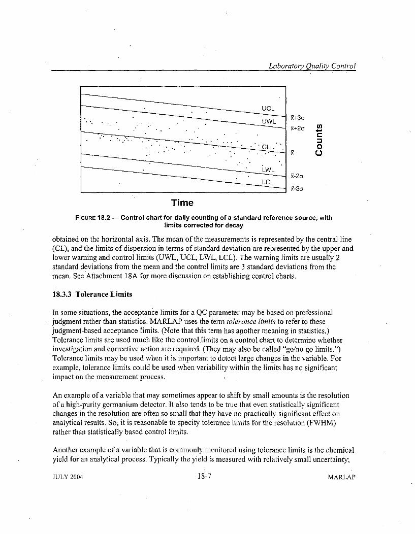
Laboratory Quality Control

UCL

""-'-"'--•UWL • 3R+2cy

• iWL

LCL

Time

FIGURE 18.2 - Control chart for daily counting of a standard reference source, withlimits corrected for decay

obtained on the horizontal axis. The mean of the measurements is represented by the central line(CL), and the limits of dispersion in terms of standard deviation are represented by the upper andlower warning and control limits (UWL, UCL, LWL, LCL). The warning limits are usually 2standard deviations from the mean and the control limits are 3 standard deviations from themean. See Attachment 18A for more discussion on establishing control charts.

18.3.3 Tolerance Limits

In some situations, the acceptance limits for a QC parameter may be based on professionaljudgment rather than statistics. MARLAP uses the term tolerance limits to refer to thesejudgment-based acceptance limits. (Note that this term has another meaning in statistics.)Tolerance limits are used much like the controllimits on a control chart to determine whetherinvestigation and corrective action are required. (They may also be called "go/no go limits.")Tolerance limits may be used when it is important to detect large changes in the variable. Forexample, tolerance limits could be used when variability within the limits has no significantimpact on the measurement process.

An example of a variable that may sometimes appear to shift by small amounts is the resolutionof a high-purity germanium detector. It also tends to be true that even statistically significantchanges in the resolution are often so small that they have no practically significant effect onanalytical results. So, it is reasonable to specify tolerance limits for the resolution (FWHM)rather than statist.ically based control 'limits.

Another example of a variable that is commonly monitored using tolerance limits is the chemicalyield for an analytical process. Typically the yield is measured with relatively small uncertainty;

JULY 2004 18-7 MARLAP

Laboratory Quality Control

so, fluctuations of the yield over some range of values may have no substantial impact on thequality of the measurement. However, a yield that is significantly greater than 100 percentgenerally indicates a spurious error of some kind, and a yield that is very low may indicate aspurious error or other problem in the measurement process that deserves investigation(seeSections 18.6.4, "Interferences"; 18.6.5, "Negative Results"; and 18.6.7, "Calibration ofApparatus Used for Weight and Volume Measurements").

A graphical representation of the history of the monitored variable is useful even when controlcharts are not used. When the data are plotted on a graph with the tolerance limits drawn as lines(like the control limits on a control chart), the graph is sometimes called a tolerance chart.

18.3.4 Measurement Uncertainty

Issue: Every measured result is uncertain to some degree. If the measurement uncertainties arelarge relative to the tolerances needed for decision making, the, data may not be useful for theirintended purpose. A discussion of measurement uncertainty is contained in Chapter 19, and theterms used in this section are defined in that chapter and in the Glossary.

Discussion: In order to determine the significance of a sample result, all reported values shouldbe accompanied by the laboratory's best estimate of the uncertainty associated with the result.The "combined standard uncertainty" (one-sigma uncertainty) is obtained by propagating theuncertainties of all the input quantities that contribute to the calculation of the derived value(Chapter 19).

The combined standard uncertainty is used to indicate the statistical confidence in interpretingthe performance indicator's ability to assess analytical quality. The estimated statistical confi-dence level that is usually associated with 1 combined standard uncertainty is about 68 percent,the confidence level for 2 combined standard uncertainties is about 95 percent, and the confi-dence level for 3 combined standard uncertainties is about 99 percent. It is important that thecombined standard uncertainty be a fair estimate because it will indicate when the analyticalprocess could be approaching the limits of statistical control and corrective actions should beinitiated. A performance indicator exceeding ±2 combined standard uncertainty limits from theindicator's historical mean value may indicate that corrective action should be considered, and aperformance indicator exceeding ±3 combined standard uncertainty limits from the indicator'shistorical mean value may indicate that an investigation must be conducted and corrective actionmay be necessary. Because statistical confidence never reaches 100 percent, it probably would beprudent to confirm the measurement for the performance indicator when it exceeds ±2 combinedstandard uncertainty limits. If the performance indicator value for repeat measurements do notexceed ±2 combined standard uncertainty limits, one may conclude that the first measurementwas a statistically allowable event. However, if the excursion is repeated, appropriate investiga-tive actions should be considered.

MARLAP 18-8 JULY 2004

Laboratoiy Quality Control

Most of the significant sources of uncertainty in radiochemical data are known to a laboratoryand can be estimated. These include uncertainties associated with sample and background count-ing, radiochemical yield determination, efficiency calibration, and blank assessment. Other lesseasily defined but significant sources of uncertainty include those associated with self-absorptionand quench correction, sample density correction, sample geometry variation, gamma photopeakarea determination, determination of sample volume or weight, and dead time correction.

The uncertainty of a measured value is controllable, within certain limits, by decreasing theuncertainty associated with some input parameters. For samples containing low levels of radio-activity, a large component of the combined standard uncertainty may be associated with theinstrumental assessment (counting) of the sample aliquant, i.e., the standard uncertainty of the netcount (gross sample count minus background count). Increasing the total net count accumulated,or decreasing the uncertainty of the instrument background, or both, will decrease the countinguncertainty. Changes that may be made to decrease the counting uncertainty include increasingthe counting time for the sample or background, increasing the sample aliquant size (unless thesample geometry, quench, or self-absorption factors offset the gain in total radioactivity counted),using a more efficient geometry or detector, using an instrument with a lower background, andreanalyzing the sample to obtain a greater radiochemical yield. It also may be possible toconcentrate the sample, which has the equivalent effect of increasing the sample aliquant size.

18.4 Radiochemistry Performance Indicators

Section 18.3 discussed how to evaluate radiochemistry performance indicators using statisticallybased control chart techniques. Any of the indicators below (blanks, replicates, laboratory controlsamples, matrix spikes, certified reference material, or tracer yield) can be evaluated using thecontrol chart techniques. Analysts can use numerical performance indicators to identify loss ofcontrol. Control charts will assist laboratory personnel in identifying the quality trends andexcursions of any performance indicator.

18.4.1 Method and Reagent Blank

Issue: A method blank is a sample of a matrix as similar as practical to the associated samplesthat is free from the analytes (radionuclides) of interest to the extent possible. The method blankis processed simultaneously with, and under the same conditions as, samples through all steps ofthe analytical procedures. A reagent blank consists of theanalytical reagent(s) in the procedurewithout the target analyte or sample matrix, introduced into the analytical procedure at theappropriate point and carried through all subsequent steps to determine the contribution of thereagents and of the involved analytical steps.

Blank samples are used to determine whether any radionuclide contamination is introduced bythe measurement process. They assist in the control of any contamination introduced by the

JULY 2004 18-9 MARLAP

Laboratory Quality Control

laboratory. Ideally, no target analytes should be present in the blank at detectable concentrations.If that is not possible (e.g., for naturally occurring radionuclides), those radionuclides should beextremely well-characterized and tracked. Control charts can be used to track these radionuclidelevels in blanks. Using X charts, the laboratory can establish a program that evaluates the levelsand trends of radionuclides in the different laboratory blanks. The techniques for establishingsuch a control chart program are described in Attachment 18A.

Discussion: The method blank is assumed to be representative of all samples in the batch withrespect to the matrix and contamination assessment. When practical, it consists of the same orequivalent medium as the analytical samples, such as a deionized water blank for aqueoussamples. Soil blanks are often prepared using "clean sand," commercially available fine-grainedor beach sand whose inherent concentrations of target radionuclides are small and have beencharacterized sufficiently by the laboratory to allow its use as a blank. This approach may not beappropriate for very low-level analyses. Powdered, natural-matrix Standard Reference Materials(SRMs) are commercially available from the National Institute of Standards and Technology(NIST) and also may be suitable (Section 18.4.5). However, due to the natural variability of soils,each choice of method blank medium must be evaluated by the laboratory prior to use. Theresults of method blanks typically are not used to correct sample activities but only to monitor forcontamination.

Reagent blanks are matrix-independent and assess any contamination only from the reagents andlab-ware. They may be used to correct sample activities for the contribution of naturallyoccurring radionuclides in the reagents, and used like method blanks, to check for unexpectedcontamination. The results of the reagent blank analyses should be reported separately by theanalytical laboratory. How their values are used in determining the final sample results should beaddressed during the final data assessment.

It is common practice for some laboratories to add the reagents into a volume of deionized waterequal to the sample volume, while other laboratories simply add the required reagents to anempty container and process it as an analytical sample. In either case, it should be noted that thereagent blank is not monitoring the entire analytical process. The fundamental issue for eachlaboratory is to decide on the appropriate reagent blank necessary to obtain the needed informa-tion on the measurement system. Considerable variability exists among laboratories in the useand preparation of reagent blanks.

In general, the reagent blank's concentration of analyte is expected to be small compared to thatof the sample. However, for some low-activity environmental samples this may not be the case,and the correction becomes increasingly important as the concentration of the analyte in thesample approaches background concentrations. In these cases, care should be taken to accuratelyquantify the levels of radionuclides in the reagent blanks.

MARLAP 18-10 JULY 2004

Laboratory Quality Control

It is important to minimize radionuclide concentrations in the blanks and bring these levels undercontrol. This is usually achieved through careful selection of reagents, maintaining laboratoryand counting areas free from contamination, and by segregating high and low activity samples.Thorough documentation of all blank values is essential to allow for the application of statisticaltests to evaluate potentially anomalous values and delineate their extent.

Ideally, the analyte concentration in a method or reagent blank should be as close to zero aspossible, and replicate measurement of the blanks should be consistent within counting statistics.Acceptance criteria for blank results should be established and applied to all data, and shouldinclude warning and control limits (Section 18.3.2, "Statistical Means of Evaluating PerformanceIndicators - Control Charts"). Blank values require scrutiny as part of the data evaluation andvalidation process for each analytical batch. Should restocking of reagents or other wholesalelaboratory changes occur during a project, the method and reagent blanks prepared under the newconditions should be re-evaluated to ensure that they continue to be within established criteria.

An example of a numerical performance indicator for a method blank or a reagent blank used tomonitor for unexpected contamination is

X

ZB-ank - UP) (18.1)

where x denotes the measured blank activity and uc(x) denotes its combined standard uncertainty.Warning limits for ZSfank are ±2 and control limits are ±3. As mentioned earlier, if a reagent blankis used to blank-correct sample results, the blank results should be evaluated using control charts.

Typically, one method blank and/or reagent blank is analyzed with each batch or grouping ofanalytical samples regardless of batch size. Situations may occur where more frequent blanks arerequired to ensure that analytical conditions are stable, particularly when analyzing high and lowconcentration samples in the same analytical batch, or when instruments, reagents, or analyticalmethod are suspect.

In general, corrective actions include procurement control of reagents, good laboratory cleaningpractices, sample segregation according to anticipated concentrations, and instrument-relatedconcerns, as discussed in this section. Good laboratory cleaning protocols should incorporate theevaluation of method and reagent blank performance to indicate if current practices are adequate.Instrument background data indicate a system's stability, and can be used to pinpoint the sourceof contamination, as can routine contamination (removable and fixed) surveys of laboratory andcounting areas that are performed by the organization's health physics or radiation safetypersonnel.

Excursion: Blank changes can be grouped into three general categories: rapid changes, gradualincrease or decrease, and highly variable changes. These are represented in Figure 18.3 anddescribed below.

JULY 2004 18-11 MARLAP

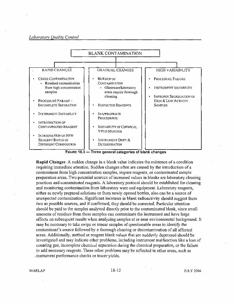
Laboratory Quality Control

I BLANK CONTAMINATION

I IRAPID CHANGES

CROSS CONTAMINATION

- Residual contaminationfrom high concentrationsamples

PROCEDURE FAILURE -

INCOMPLETE SEPARATION

* INSTRUMENT INSTABILITY

* INTRODUCTION OF

CONTAMINATED REAGENT

INTRODUCTION OF NEWREAGENT BATCH OF

DIFFERENT COMPOSITION

GRADUAL CHANGES

" BUILDUP OF

CONTAMINATION

- Glassware/laboratoryareas require thoroughcleaning

" SUSPECTED REAGENTS

" INAPPROPRIATE

PROCEDURES

" INSTABILITY OF CHEMICAL

YIELD MONITOR

" INSTRUMENT DRIFT &

DETERIORATION

HIGH VARIABILITY

" PROCEDURE FAILURE

" INSTRUMENT INSTABILITY

" IMPROPER SEGREGATION OFHIGH & Low ACTIVITYSAMPLES

FIGURE 18.3 - Three general categories of blank changes

Rapid Changes: A sudden change in a blank value indicates the existence of a conditionrequiring immediate attention. Sudden changes often are caused by the introduction of acontaminant from high concentration samples, impure reagents, or contaminated samplepreparation areas. Two potential sources of increased values in blanks are laboratory cleaningpractices and contaminated reagents. A laboratory protocol should be established for cleaningand monitoring contamination from laboratory ware and equipment. Laboratory reagents,either as newly prepared solutions or from newly opened bottles, also can be a source ofunexpected contamination. Significant incre~ases in blank radioactivity should suggest thesetwo as possible sources, and if confirmed, they should be corrected. Particular attentionshould be paid to the samples analyzed directly prior to the contaminated blank, since smallamounts of residues from these samples can contaminate the instrument and have largeeffects on subsequent results when analyzing samples at or near environmental background. Itmay be necessary to take swipe or smear samples of questionable areas to identify thecontaminant's source followed by a thorough cleaning or decontamination of all affectedareas. Additionally, method or reagent blank values that are suddenly depressed should beinvestigated and may indicate other problems, including instrument malfunction like a loss ofcounting gas, incomplete chemical separation during the chemical preparation, or the failureto add necessary reagents. These other problems may be reflected in other areas, such as

,-instrument performance checks or tracer yields.

MARLAP 18-12 JULY 2004

Laboratory Quality Control

Gradual Changes: Gradually increasing blank values indicate the need to inspect all samplepreparation and counting areas for sources of residual contamination. Often housekeeping orroutine contamination control details such as cleaning glassware or instrument countingchambers are sufficient to bring blank values under control. Alternatively, gradually decreas-ing blank values warrant scrutiny with respect to proper instrument settings and proceduralrelated problems like a lack of tracer/sample exchange, failure of chemical separation reac-tions, or the addition of all necessary reagents. The importance of documenting method andreagent blank values in this regard cannot be overemphasized, since data evaluation andtrending analyses are impossible without complete records.

High Variability: Because method blank values are expected to be near zero, the degree ofvariability they exhibit should reflect the statistical variation inherent in determinations nearthese levels. Large variations in blank values typically indicate problems related toinstruments or the analytical process, as discussed in the two previous sections.

18.4.2 Laboratory Replicates

Issue: A laboratory replicate is two or more aliquants taken at the first subsampling event,normally after homogenization. In the event that there is no subsampling (when the method callsfor using the entire sample) replicate analysis typically involves counting the prepared sampletwice. The results of laboratory replicates are used to evaluate the method precision. Note thatcounting a sample twice only assesses the instrument portion of the measurement process.

Precision is a measure of agreement among replicate measurements of the same property underprescribed similar conditions. Precision is a fundamental aspect of the analytical process andshould be evaluated routinely as part of the laboratory's quality system. Evaluation typically isperformed using multiple analysis of the same sample (blanks, spikes, blinds, referencematerials, performance evaluation samples, etc.), in whole or part, and evaluating the analysesrelative to a statistically based criterion. The range of sample types requires that the samplematrix's effects on the precision be captured and evaluated by the laboratory's routine qualitycontrol practices. The reproducibility of analytical results should be evaluated by replicates toestablish this uncertainty component.

Discussion: The purpose for measuring precision is to determine whether the laboratory canexecute an analytical method consistently and thus obtain results of acceptable variability.Analytical samples cover a range of physical forms or matrices, from homogeneous samples likefinished drinking water to complex soils or heterogeneous wastes, and each matrix has thepotential to affect a protocol's precision.

In general, precision for aqueous samples tends to be less affected by sample heterogeneity thanother media because if the sample's constituents are dissolved the sample is essentially homo-

JULY 2004 18-13 MARLAP

Laboratory Quality Control

geneous. This facilitates dividing the samples into equivalents fractions or aliquants. Whenappropriate, acidification of a sample to pH less than 2 should be done prior to dividing it forreplicate analysis. Multi-phase and high-solid-content samples that are heterogeneous are moreproblematic.

The acceptance criterion for precision should be related to the combined standard uncertainties ofthe measured results. The uncertainty of a result may depend on many factors (e.g., dissolvedsolids in water or particle sizes of soil), but such factors should affect the acceptance criteriononly through their effect on the standard uncertainty.

As an alternative to sample duplicates, a matrix spike duplicate is sometimes used as an indicatorof the reproducibility of the analytical precision, as discussed in Section 18.4.3. A matrix spikeduplicate is treated in the same manner as an unspiked replicate: both samples (original andduplicate) are processed identically to the other samples in the batch, and each aliquant is treatedas an individual sample.

If the sample has multiple phases, the phases should be separated for individual analysis. Forheterogenous materials, multiple analyses should be used, or the combined standard uncertaintyof the results should be increased, to account for subsampling error (Appendix F). A typicalfrequency for replicate analyses is a minimum of one per analytical batch, regardless of batchsize. "Batch" is defined as a given number of samples of similar matrix type with associated QCsamples analyzed under the sample conditions at approximately the same time.

All analytical batches should be evaluated with respect to precision, whether by using replicatesor matrix spike duplicates. This is done typically by the use of an acceptance criterion thatderives a statistic that quantifies the difference between two values obtained by analyzing thesame sample. Limits are then placed on the criterion, and data for any batch in excess of thecriterion require investigation and corrective action as appropriate. An example of a numerical

,performance indicator for laboratory replicates isX I - X 2

ZRep 2 () 2 (18.2)u I(X2)

where x, and x2 denote the two measured activity concentrations and u,(x,) and Uc(X 2) denote theirrespective combined standard uncertainties. Warning limits for ZRCp are ±2 and control limitsare ±3.

Excursions: A regularly scheduled evaluation of precision with respect to the acceptancecriterion should be an integral part of the laboratory quality system. Careful attention should bepaid to the nature and anticipated analyte concentrations of all samples processed by the labora-tory. Prospective identification of samples where precision is expected to be problematic often

MARLAP 18-14 JULY 2004

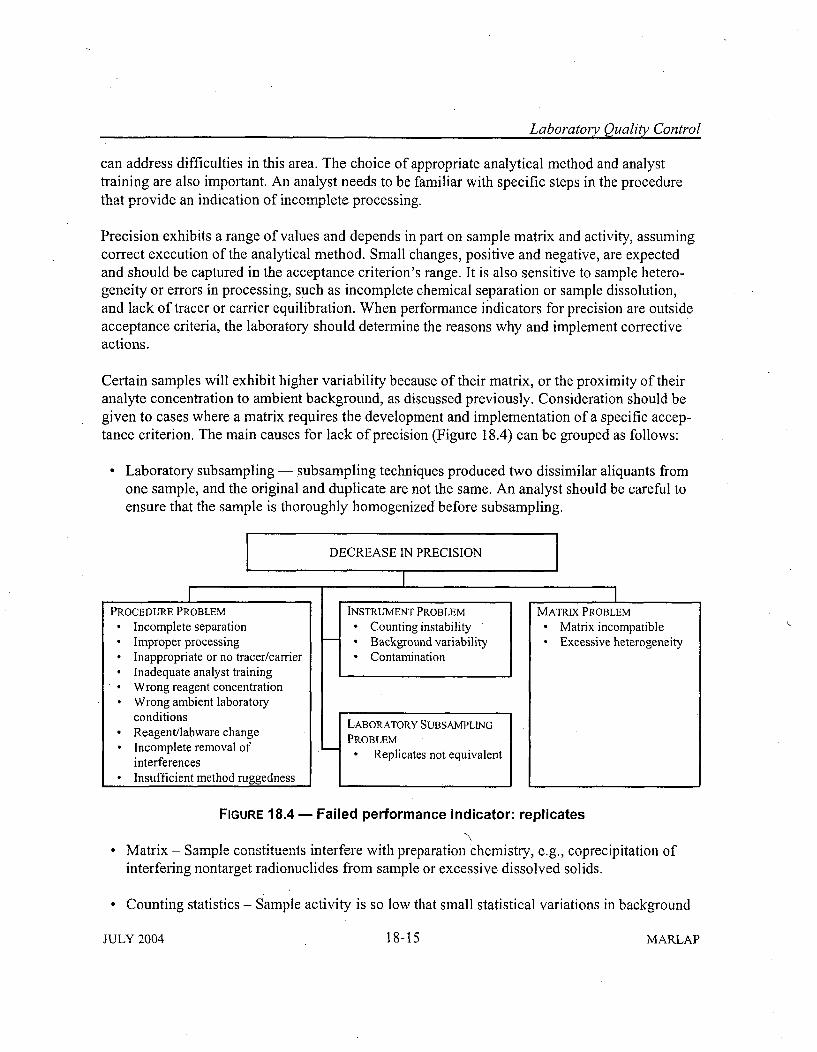
Laboratoiy Quality Control

can address difficulties in this area. The choice of appropriate analytical method and analysttraining are also important. An analyst needs to be familiar with specific steps in the procedurethat provide an indication of incomplete processing.

Precision exhibits a range of values and depends in part on sample matrix and activity, assumingcorrect execution of the analytical method. Small changes, positive and negative, are expectedand should be captured in the acceptance criterion's range. It is also sensitive to sample hetero-geneity or errors in processing, such as incomplete chemical separation or sample dissolution,and lack of tracer or carrier equilibration. When performance indicators for precision are outsideacceptance criteria, the laboratory should determine the reasons why and implement correctiveactions.

Certain samples will exhibit higher variability because of their matrix, or the proximity of theiranalyte concentration to ambient background, as discussed previously. Consideration should begiven to cases where a matrix requires the development and implementation of a specific accep-tance criterion. The main causes for lack of precision (Figure 18.4) can be grouped as follows:

Laboratory subsampling - subsampling techniques produced two dissimilar aliquants fromone sample, and the original and duplicate are not the same. An analyst should be careful toensure that the sample is thoroughly homogenized before subsampling.

DECREASE IN PRECISION

PROCEDURE PROBLEM" Incomplete separation" Improper processing" Inappropriate or no tracer/carrier" Inadequate analyst training. Wrong reagent concentration" Wrong ambient laboratory

conditions" Reagent/labware change" Incomplete removal of

interferences" Insufficient method ruggedness

HINSTRUMENT PROBLEM

" Counting instability" Background variability" Contamination

MATRIX PROBLEM" Matrix incompatible" Excessive heterogeneity

I LABORATORY SUBSAMPLING

PROBLEMReplicates not equivalent

FIGURE 18.4 - Failed performance indicator: replicates

M.t....... - Sample constiuents" iefere with preparation chcmistry, e.g., coprecipitation ofinterfering nontarget radionuclides from sample or excessive dissolved solids.

* Counting statistics - Sample activity is so low that small statistical variations in background

JULY 2004 18-15 MARLAP

Laboratory Quality Control

cause disproportionate responses.

" Contamination - Intermittent contamination from measurements system, glassware, etc.,produces anomalous data for the original sample, but not the duplicate/replicate.

" Other - Failed chemical process, failed instrumentation, training, failed lab environment,failed procurement control.

18.4.3 Laboratory Control Samples, Matrix Spikes, and Matrix Spike Duplicates

Issue: A laboratory control sample (LCS) is a QC sample of known composition (referencematerial) or an artificial sample, created by fortifying a clean material similar in nature to theenvironmental sample. The LCS is prepared and analyzed in the same manner as the environ-mental sample. A matrix spike is typically an aliquant of a sample fortified (spiked) with knownquantities of target radionuclides and subjected to the entire analytical procedure to establish ifthe method or procedure is appropriate for the analysis of a particular matrix. In some cases,specifically prepared samples of characterized materials that contain or are spiked with the targetradionuclide and are consistent with the sample matrix may be used as matrix spikes. Matrixspikes should be used for those methods that do not include a radiotracer or internal carrier in thechemical separation process and where there is sufficient sample. A matrix spike duplicate(MSD) is a second-replicate matrix spike that is used to evaluate the method precision. Matrixspike duplicates are used in a similar fashion as laboratory sample replicates, but in cases wherethere are insufficient quantities of target radionuclides in the laboratory sample replicates toprovide statistically meaningful results.

An important performance indicator is the ability to ensure that the analytical methods employedobtain data that are representative of the true activity in a sample, i.e., produce data that areaccurate. The routine analysis of spiked samples provide data for an evaluation of the labora-tory's reported measurement uncertainty and allow for the determination of bias, if one exists.Evaluation is typically performed using prepared samples consisting of media equivalent to aroutine analytical sample with a known, measurable amount of the analyte of interest. Uponcompletion of the analysis, the results are compared to the known or accepted value, and theagreement is evaluated using a. predetermined criterion. The range of sample types assayed in alaboratory may require the preparation of spikes using several sample media. Use of matrixspiked samples will reflect the analytical method's ability to make accurate quantitativedeterminations in the presence of the matrix.

Discussion: As stated previously, analytical samples cover a range of physical forms or matrices,and each matrix can change a meto ''s expected accuracy. Tracking sets of LCS and matrixspike results can give laboratory personnel an indication of the magnitude of an observed methodbias. Care must be taken when analyzing site specific matrix spike results because these matrices

MARLAP 18-16 JULY 2004

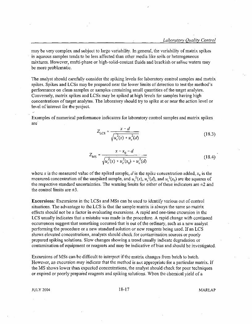
Laboratory Quality Control

may be very complex and subject to large variability. In general, the variability of matrix spikesin aqueous samples tends to be less affected than other media like soils or heterogeneousmixtures. However, multi-phase or high-solid-content fluids and brackish or saline waters maybe more problematic.

The analyst should carefully consider the spiking levels for laboratory control samples and matrixspikes. Spikes and LCSs may be prepared near the lower limits of detection to test the method'sperformance on clean samples or samples containing small quantities of the target analytes.Conversely, matrix spikes and LCSs may be spiked at high levels for samples having highconcentrations of target analytes. The laboratory should try to spike at or near the action level orlevel of interest for the project.

Examples of numerical performance indicators for laboratory control samples and matrix spikesare

ZLCs = / 2 j (18.3)'(x) + u (d)

zMS u(X) + u(X) u2(d) (18.4)

where x is the measured value of the spiked sample, d is the spike concentration added, x0 is themeasured concentration of the unspiked sample, and uC2(x), u 2(d), and uC2(xo) are the squares ofthe respective standard uncertainties. The warning limits for either of these indicators are ±2 andthe control limits are +3.

Excursions: Excursions in the LCSs and MSs can be used to identify various out of controlsituations. The advantage to the LCS is that the sample matrix is always the same so matrixeffects should not be a factor in evaluating excursions. A rapid and one-time excursion in theLCS usually indicates that a mistake was made in the procedure. A rapid change with continuedoccurrences suggest that something occurred that is out of the ordinary, such as a new analystperforming the procedure or a new standard solution or new reagents being used. If an LCSshows elevated concentrations, analysts should check for contamination sources or poorlyprepared spiking solutions. Slow changes showing a trend usually indicate degradation orcontamination of equipment or reagents and may be indicative of bias and should be investigated.

Excursions of MSs can be difficult to interpret if the matrix changes from batch to batch.However, an excursion may indicate that the method is not appropriate for a particular matrix. Ifthe MS shows lower than expected concentrations, the analyst should check for poor techniquesor expired or poorly prepared reagents and spiking solutions. When the chemical yield of a

JULY 2004 18-17 MARLAP

Laboratory Quality Control

process is determined through a stable isotopic carrier, lower-than-expected analyte concentra-tions may result from inherent quantities of the stable isotope in the sample matrix.

Elevated or depressed results for site-specific MSs need to be interpreted in conjunction with theresults from LCSs. If both the LCS and site-specific MS results are elevated or depressed thenthe cause is usually internal to the laboratory. If only the site-specific MS is depressed orelevated, the cause usually is due to the matrix.

18.4.4 Certified Reference Materials

Issue: Certified reference materials (CRMs) are well-characterized, stable, homogeneousmaterials with physical or chemical properties that are known within specified uncertainty limits.Laboratories that analyze CRMs can compare their performance to the certified concentrationand uncertainty levels. CRMs are used for the calibration of an apparatus or the assessment of ameasurement method.

Discussion: Metrology organizations issue CRMs in various matrices with critically evaluatedconcentration values for the radionuclide constituents. A CRM issued by NIST or under licensefrom NIST is called a "standard reference material" (SRM). The usefulness of a referencematerial depends on the characterization of the radionuclide source, activity levels, and theirestimated uncertainties.

CRMs can be used as internal laboratory QC samples to evaluate the ability of analytical methodsto handle the matrix. CRMs need not be known to the analyst but can be introduced into theanalytical stream as a blind. Comparison of analytical results of CRMs to their certified valuesprovides linkage to the NIST radioactivity primary standards and a measure of method accuracy.

The planning that goes into the preparation of a CRM involves the selection of analyticaltechniques that have adequate sensitivity and precision for specific analyses. It has becomeincreasingly important to have available well-characterized CRMs of a natural "matrix" type,which may be used in laboratory tests of measurements of environmental radioactivity. Suchmaterials may be used in the evaluation of competing analytical methods, and also in thecross-comparison of interlaboratory data-both at the national level and the international level.

The Ionizing Radiation Division of NIST has constructed several SRMs for radiation measure-ments. These are included in the 4350 series and can be ordered through NIST. One widely usedSRM is the natural matrix ocean sediment (4357). The radionuclides in the NIST natural matrixSRMs are not spiked into the matrix but are incorporated through natural processes to present theanalyst with the combination of species that may be faced on a routine basis. SRM 4357 has twosediment sources: the Chesapeake Bay (benign) and the Irish Sea ("hot").

MARLAP 18-18 JULY 2004

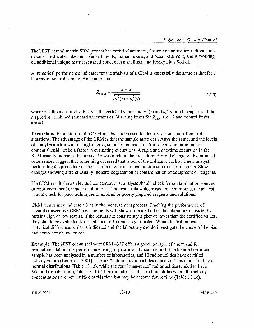
Laboratory Quality Control

The NIST natural matrix SRM project has certified actinides, fission and activation radionuclidesin soils, freshwater lake and river sediments, human tissues, and ocean sediment, and is workingon additional unique matrices: ashed bone, ocean shellfish, and Rocky Flats Soil-fl.

(

A numerical performance indicator for the analysis of a CRM is essentially the same as that for alaboratory control sample. An example is

ZCRM= xu d 2 (18.5)

where x is the measured value, d is the certified value, and u,2(x) and uc2(d) are the squares of therespective combined standard uncertainties. Warning limits for ZcRM are +2 and control limitsare ±3.

Excursions: Excursions in the CRM results can be used to identify various out-of-controlsituations. The advantage of the CRM is that the sample matrix is always the same, and the levelsof analytes are known to a high degree, so uncertainties in matrix effects and radionuclidecontent should not be a factor in evaluating excursions. A rapid and one-time excursion in theSRM usually indicates that a mistake was made in the procedure. A rapid change with continuedoccurrences suggest that something occurred that is out of the ordinary, such as a new analystperforming the procedure or the use of a new batch of calibration solutions or reagents. Slowchanges showing a trend usually indicate degradation or contamination of equipment or reagents.

If a CRM result shows elevated concentrations, analysts should check for contamination sourcesor poor instrument or tracer calibration. If the results show decreased concentrations, the analystshould check for poor techniques or expired or poorly prepared reagents- and solutions.

CRM results may indicate a bias in the measurement process. Tracking the performance ofseveral consecutive CRM measurements will show if the method or the laboratory consistentlyobtains high or low results. If the results are consistently higher or lower than the certified values,they should be evaluated for a statistical difference, e.g., t-tested. When the test indicates astatistical difference, a bias is indicated and the laboratory should investigate the cause of the biasand correct or characterize it.

Example: The NIST ocean sediment SRM 4357 offers a good example of a material forevaluating a laboratory performance using a specific analytical method. The blended sedimentsample has been analyzed by a number of laboratories, and 10 radionuclides have certifiedactivity values (Lin et al., 2001). The six "natural" radionuclides concentrations tended to have.normal distributions (Table 18. !a), while the four "man-made" radionuclides tended to haveWeibull distributions (Table 18. lb). There are also 11 other radionuclides where the activityconcentrations are not certified at this time but may be at some future time (Table 18.1 c).

JULY 2004 18-19 MARLAP

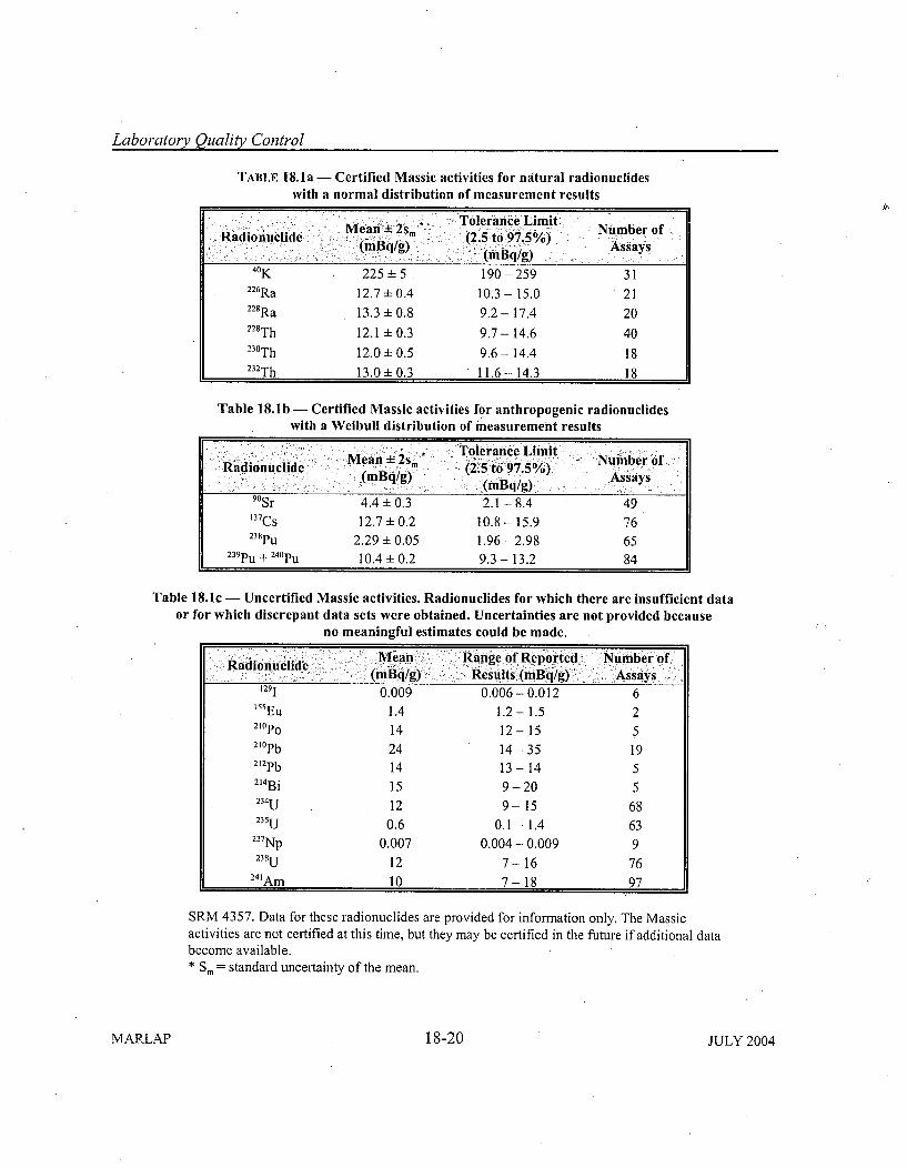
Laboratory Quality Control

TABLE 18.1a - Certified Massic activities for natural radionuclideswith a normal distribution of measurement results

Me•an ± 2 Nu Tolerance Limit Nme of.Radionuclide ,=. ,. . (2.5 to, 97.5%0),' Assays(mqg) ... (mBqAg)

40K 225 5 190-259 31

226Ra 12.7 - 0.4 10.3- 15.0 21228Ra 13.3 - 0.8 9.2- 17.4 20228Th 12.1 -0.3 9.7- 14.6 40230Th 12.0 0.5 9.6- 14.4 18232Th 13.0 -0.3 11.6- 14.3 18

Table 18.1b- Certified Massic activities for anthropogenic radionuclideswith a Weibull distribution of measurement results

can= ,, :• , :"Tolerance Limit Numb. of: •:,•.• = :,• . M :vea~n=4 ± s 2S ,• :: Number of •Radionuclide M 2,0 (2.5 to 97.5%) Ass.ys... .. "(mt~q/g): Assays

(m~q/g)(mBq/g),90Sr 4.4 0.3 2.1-8.4 49t37Cs 12.7 + 0.2 10.8- 15.9 76238

pu 2.29 0.05 1.96-2,98 652 3 9

pu + 24 0

pu 10.4 - 0.2 9.3- 13.2 84

Table 18.1c - Uncertified Massic activities. Radionuclides for which there are insufficient dataor for which discrepant data sets were obtained. Uncertainties are not provided because

no meaningful estimates could be made.Radionuclide Mean,.: Range of Reported . Number, of

(mBq/g) , Results (mBq/g) :. Assays1291 0.009 0.006 - 0.012 6

155Eu 1.4 1.2- 1.5 221Po 14 12- 15 52 rpb 24 14-35 19212Pb 14 13-14 5214Bi 15 9-20 5234u 12 9-15 68235u 0.6 0.1-1.4 63

237Np 0.007 0.004 - 0.009 9

2 38u 12 7-16 76

24'Am 10 7- 18 97

SRM 4357. Data for these radionuclides are provided for information only. The Massicactivities are not certified at this time, but they may be certified in the future if additional databecome available.* Sm = standard uncertainty of the mean.

MARLAP 18-20 JULY 2004

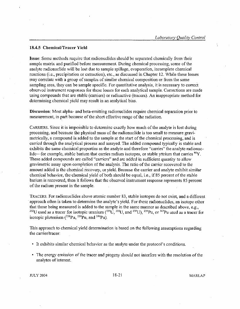
Laboratoty Quality Control

18.4.5 Chemical/Tracer Yield

Issue: Some methods require that radionuclides should be separated chemically from theirsample matrix and purified before measurement. During chemical processing, some of theanalyte radionuclide will be lost due to sample spillage, evaporation, incomplete chemicalreactions (i.e., precipitation or extraction), etc., as discussed in Chapter 12. While these lossesmay correlate with a group of samples of similar chemical composition or from the samesampling area, they can be sample specific. For quantitative analysis, it is necessary to correctobserved instrument responses for these losses for each analytical sample. Corrections are madeusing compounds that are stable (carriers) or radioactive (tracers). An inappropriate method fordetermining chemical yield may result in an analytical bias.

Discussion: Most alpha- and beta-emitting radionuclides require chemical separation prior tomeasurement, in pat because of the short effective range of the radiation.

CARRIERS. Since it is impossible to determine exactly how much of the analyte is lost duringprocessing, and because the physical mass of the radionuclide is too small to measure gravi-metrically, a compound is added to the sample at the start of the chemical processing, and iscarried through the analytical process and assayed. The added compound typically is stable andexhibits the same chemical properties as the analyte and therefore "carries" the analyte radionuc-lide-for example, stable barium that carries radium isotopes, or stable yttrium that carries 90Y.These added compounds are called "carriers" and are added in sufficient quantity to allowgravimetric assay upon completion of the analysis. The ratio of the carrier recovered to theamount added is the chemical recovery, or yield. Because the carrier and analyte exhibit similarchemical behavior, the chemical yield of both should be equal, i.e., if 85 percent of the stablebarium is recovered, then it follows that the observed instrument response represents 85 percentof the radium present in the sample.

TRACERS. For radionuclides above atomic number 83, stable isotopes do not exist, and a differentapproach often is taken to determine the analyte's yield. For these radionuclides, an isotope otherthat those being measured is added to the sample in the same manner as described above, e.g.,232U used as a tracer for isotopic uranium (234U, "35U, and 238U), 236pu, or 242Pu used as a tracer forisotopic plutonium (238Pu, 239Pu, and 24°pu).

This approach to chemical yield determination is based on the following assumptions regardingthe carrier/tracer:

" It exhibits similar chemical behavior as the analyte under the protocol's conditions.

" The energy emission of the tracer and progeny should not interfere with the resolution of theanalytes of interest.

JULY 2004 18-21 MARLAP

Laboratory Quality Control

" It is chemically and physically equilibrated with the sample before losses of either occur.

• Indigenous concentrations of carrier or tracer are insignificant, or are well known and can bequantified and corrected for during subsequent data analysis.

" The chemical form of carrier or tracer precipitates are consistent with what was used duringthe material's preparation and standardization.

Care should be taken during the analytical procedure to ensure that these assumptions are valid.Different conditions, such as a lack of equilibrium between .the tracer and sample analyte, canresult in inaccurate data. If there is indigenous tracer or carrier in the sample, this quantity shouldbe known so that the appropriate correction can be made for its contribution to the chemicalyield. In some cases, this will prevent the procedure's use, as described below. As statedpreviously, the quantity of tracer or carrier added to the sample should overwhelm its indigenousconcentration, which cannot be determined for samples with unknown tracer or carrier content. Aseparate analysis for trace elements or interfering radionuclides could provide information toestimate the uncertainty contributed by the sample's indigenous tracer or carrier.

It should be noted that some analytical methods exclude direct assessment of the procedure'schemical yield for each sample analysis. In such cases, chemical yield typically recovery isaddressed by analyzing a group of prepared standards by the same protocol and the results areanalyzed statistically to derive a chemical yield factor. The recovery factor is applied to routinesamples based on the assumption that the standards used for its derivation are representative ofroutine samples. This approach precludes the empirical assessment of a sample specific chemicalyield, and would probably require scrutiny and periodic verification.

Acceptance limits for chemical/tracer yields should be specified in the laboratory's qualitymanual. While it is customary to establish lower limits for chemical yield, upper limits may alsobe necessary since excessive yields indicate a loss of analytical control. All limits developed bythe laboratory should be either statistically based or based on historical data, and should includewarning and control limits. The inherent differences among sample matrices generally require theuse of matrix specific criteria, i.e., finished drinking whater limits may differ from limits for highsolid content waters, sandy soils or heterogeneous media. Irrespective of medium, wherepractical, the chemical yield and its uncertainty should be determined, recorded and tracked foreach radiochemical measurement.

Excursions: There are several possible reasons for the yield to be outside of the acceptancelimits. These are summarized in Figure 18.5 and discussed below.

MARLAP 18-22 JULY 2004

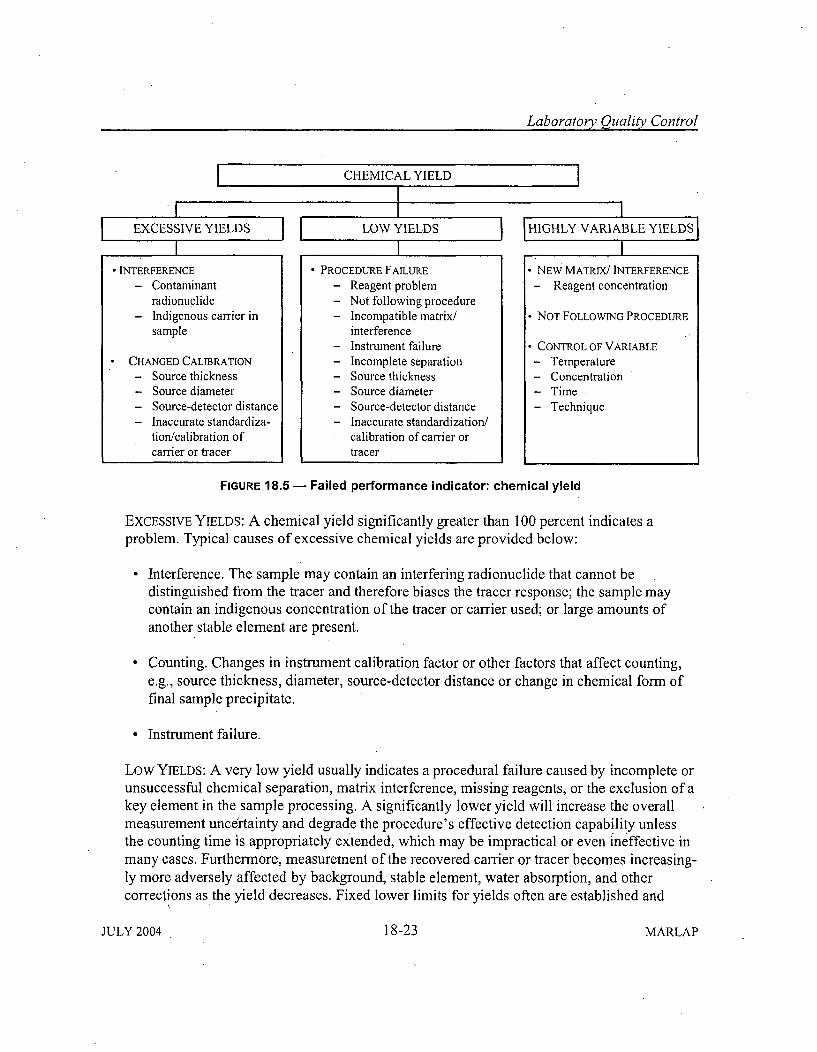
Laboratory Quality Control

I CHEMICAL YIELDi :4:I = ! . • ! .

EXCESSIVE YIELDS II LOW YIELDS HIGHLY VARIABLE YIELDS! ! ! E I

- INTERFERENCE

- Contaminantradionuclide

- Indigenous carrier insample

CHANGED CALIBRATION

- Source thickness- Source diameter- Source-detector distance- Inaccurate standardiza-

tion/calibration ofcarrier or tracer

* PROCEDURE FAILURE- Reagent problem- Not following procedure- Incompatible matrix/

interference- Instrument failure- Incomplete separation- Source thickness- Source diameter- Source-detector distance- Inaccurate standardization/

calibration of carrier ortracer

" NEW MATRIX/ INTERFERENCE- Reagent concentration

" NOT FOLLOWING PROCEDURE

" CONTROL OF VARIABLE

- Temperature- Concentration- Time,- Technique

FIGURE 18.5 - Failed performance indicator: chemical yield

EXCESSIVE YIELDS: A chemical yield significantly greater than 100 percent indicates aproblem. Typical causes of excessive chemical yields are provided below:

" Interference. The sample may contain an interfering radionuclide that cannot bedistinguished from the tracer and therefore biases the tracer response; the sample maycontain an indigenous concentration of the tracer or carrier used; or large amounts ofanother stable element are present.

" Counting. Changes in instrument calibration factor or other factors that affect counting,e.g., source thickness, diameter, source-detector distance or change in chemical form offinal sample precipitate.

" Instrument failure.

Low YIELDS: A very low yield usually indicates a procedural failure caused by incomplete orunsuccessful chemical separation, matrix interference, missing reagents, or the exclusion of akey element in the sample processing. A significantly lower yield will increase the overallmeasurement uncertainty and degrade the procedure's effective detection capability unlessthe counting time is appropriately extended, which may be impractical or even ineffective inmany cases. Furthermore, measurement of the recovered carrier or tracer becomes increasing-ly more adversely affected by background, stable element, water absorption, and othercorrections as the yield decreases. Fixed lower limits for yields often are established and

JULY 2004 18-23 MARLAP

Laboratory Quality Control

should be specific to analytical procedures and sample matrices. Setting an upper limit isrecommended for the acceptable relative uncertainty in a yield measurement.

HIGHLY VARIABLE YIELDS: High variability in procedural temperature, concentration, time,reagent concentration, or laboratory technique can have dramatic effects on yield. Highlyvariable yields indicate a lack of procedural control and should be investigated and corrected.A simple step such as heating samples on a hotplate can lead to variability in yield becausethe hotplate surface is thermally uneven. Samples can be dried and reconstituted severaltimes during the course of the preparation protocol, and samples may require differentamounts of heat or water, which introduces additional variability. When highly variablechemical yields are observed, a careful examination of the analytical procedure's applicationis recommended to determine critical variables and the controls needed to re-establishadequate management over yields.

18.5 Instrumentation Performance Indicators

Radiometric and non-radiometric instruments are used currently to quantify radionuclides in avariety of environmental matrices, and quality control measures are necessary to ensure properinstrument performance. This section presents radiometric instrument performance measures thatindicate a measurement system is in control. For detailed information on instrument concepts andspecific techniques, see Chapter 15 as well as ASTM standard practices (e.g., D3648, for theMeasurement of Radioactivity). The specific quality control procedures to be followed depend onthe measurement equipment. Sufficient checks are needed to demonstrate that the measurementequipment is properly calibrated, the appropriate background has been recorded, and that allsystem components are functioning properly. QC measures for instrumentation should include ata minimum: (1) instrument background measurements, (2) instrument calibration with referencestandards, and (3) periodic instrument performance checks subsequent to the calibration.Acceptable control limits should be specified in appropriate laboratory documents.

18.5.1 Instrument Background Measurements

Issue: In general, radionuclide detection covers more than 17 orders of magnitude of sampleactivity, from irradiated material that produces high radiation fields to environmental samples.All radiation detection instruments have a background response even in the absence of a sampleor radionuclide source. To determine the instrument's response to the radioactivity contributedby the sample alone (net), the instrument background response is subtracted from the sample-plus-background response (gross). Background corrections become more critical when theinstrument net response is small relative to the background. Careful control of contamination androutine monitoring of instrument background are therefore integral parts of a control' program.Inappropriate background correction results in analytical error and will increase the uncertaintyof data interpretation.

MARLAP 18-24 JULY 2004

Laboratory Quality Control

Discussion: Every radionuclide detector produces a signal response in the absence of a sample orradionuclide source. These signals are produced by electronic dark current, cosmic radiation,impurities in the instrument construction materials, crosstalk between the detector's alpha andbeta channels, sources in the general vicinity of the detector, and residual contamination fromprevious counting episodes. The majority of these contributors (i.e., dark current, cosmicradiation, construction material impurities) to instrument background produce a fairly constantcount rate, given sufficient measurement time. For other sources, instrument backgrounds vary asa function of time (i.e., from decay or ingrowth of residual contamination or as radon levelsfluctuate throughout the day and season). For low-level measurements, it is imperative that thebackground be maintained as low as feasible. Active or passive detector shielding, removing oradequately shielding radioactive sources in the vicinity of the detector, and good laboratorypractices to prevent residual contamination are necessary to maintain low instrument background.

The instrument's background should be determined in the absence of a radionuclide source. Theinstrument background should be well characterized. The instrument background is an importantfactor in determining the ability to achieve a specific minimum detectable concentration (MDC).Control limits for the background should be specified in appropriate laboratory documents. Thebackground population considered in the statistical calculations should cover a sufficient periodof time to detect gradual shifts in the measurement system's background contamination or detec-tor instability. Additionally, backgrounds should be determined in such a way that they mimicactual sample measurement conditions as closely as possible, i.e., using appropriate samplecontainers, geometries, and counting times.

Background measurements should be made on a regular basis and monitored using controlcharts. For instruments with well established background performance records and a lowprobability of detector contamination, this frequency may be modified by the laboratory. Formass spectrometry and kinetic phosphorimetry analysis, background measurements should beperformed on a real time basis. See ASTM E181, ANSI N42.12, and NELAC (2002) QualitySystems Appendix D for more information on the suggested frequency of backgroundmeasurement.

Excursions: Variations in instrument backgrounds may indicate instrument malfunction. Variationsmay take the form of rapid increase or decrease in background, slow increase or decrease in back-grounds, and highly variable or erratic backgrounds. These variations can result in the measurementsystem's reduced precision and decreased detection capability. Rapid or significant increases inbackground measurements may be due to instrument or blank contamination, insufficient shielding withrelocation of nearby radionuclide sources, or large scale equipment malfunction (e.g., a broken windowon a gas proportional system).

Instrument background data should be evaluated for trends, which is facilitated by regular inspec-tion of control charts. A slowly changing background could alert laboratory personnel to apotentially serious instrument failure. A sufficient number of data points (Chapter 15) taken over

JULY 2004 18-25 MARLAP

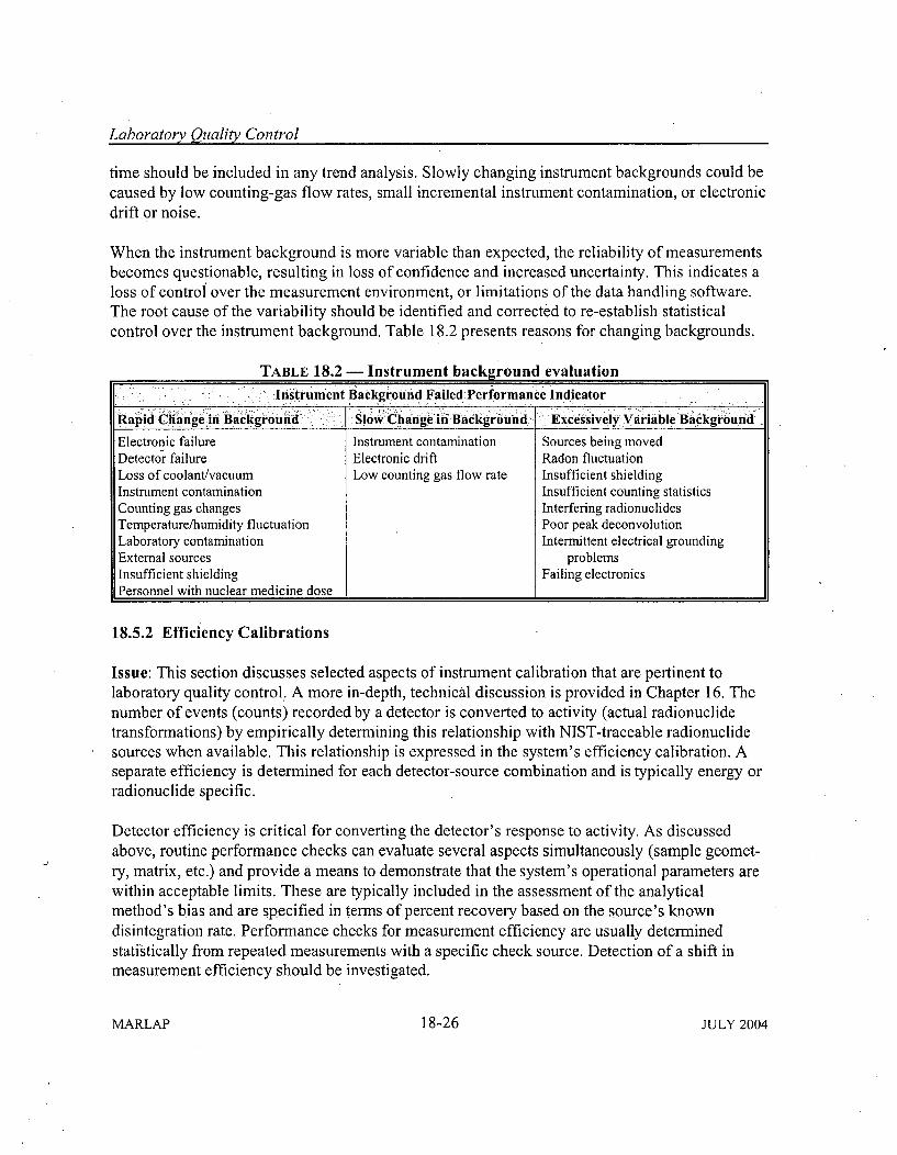
Laboratory Quality Control

time should be included in any trend analysis. Slowly changing instrument backgrounds could becaused by low counting-gas flow rates, small incremental instrument contamination, or electronicdrift or noise.

When the instrument background is more variable than expected, the reliability of measurementsbecomes questionable, resulting in loss of confidence and increased uncertainty. This indicates aloss of control over the measurement environment, or limitations of the data handling software.The root cause of the variability should be identified and corrected to re-establish statisticalcontrol over the instrument background. Table 18.2 presents reasons for changing backgrounds.

TABLE 18.2 - Instrument background evaluation,Instrument Background Failed:Performance Indicator

Rapid Change in Background. Slow Change in Background ExcessivelyVariable Background

Electronic failure Instrument contamination Sources being movedDetector failure Electronic drift Radon fluctuationLoss of coolant/vacuum Low counting gas flow rate Insufficient shieldingInstrument contamination Insufficient counting statisticsCounting gas changes Interfering radionuclidesTemperature/humidity fluctuation Poor peak deconvolutionLaboratory contamination Intermittent electrical groundingExternal sources problemsInsufficient shielding Failing electronicsPersonnel with nuclear medicine dose 1

18.5.2 Efficiency Calibrations

Issue: This section discusses selected aspects of instrument calibration that are pertinent tolaboratory quality control. A more in-depth, technical discussion is provided in Chapter 16. Thenumber of events (counts) recorded by a detector is converted to activity (actual radionuclidetransformations) by empirically determining this relationship with NIST-traceable radionuclidesources when available. This relationship is expressed in the system's efficiency calibration. Aseparate efficiency is determined for each detector-source combination and is typically energy orradionuclide specific.

Detector efficiency is critical for converting the detector's response to activity. As discussedabove, routine performance checks can evaluate several aspects simultaneously (sample geomet-ry, matrix, etc.) and provide a means to demonstrate that the system's operational parameters arewithin acceptable limits. These are typically included in the assessment of the analyticalmethod's bias and are specified in terms of percent recovery based on the source's knowndisintegration rate. Performance checks for measurement efficiency are usually determinedstatistically from repeated measurements with a specific check source. Detection of a shift inmeasurement efficiency should be investigated.

MARLAP 18-26 JULY 2004

Laboratory Qualit, Control

The frequency of performance checks for efficiency calibrations is instrument specific. Thefrequency of these checks is often based on a standardized time scale or a percentage of the totalnumber of analyses performed using that method.

Performance checks for instrument efficiency typically are performed on a day-of-use basis. Thelevel of activity in the check source should be sufficient to allow the accumulation of enoughcounts in a short time so that daily performance checks do not impose an unnecessary burden onthe laboratory. However, the source strength for spectrometry systems should be such thatinstrument dead time is not significant and gain shifts do not occur (ANSI 42.23). For detectorsthat are used infrequently, it may be necessary to perform a check before and after each set ofmeasurements.

Control charts provide a useful tool for documenting and evaluating performance checks forefficiency calibrations, and should be established and maintained for the intrinsic efficiency ofeach detector. There are several methods available for evaluating performance using controlcharts (see Attachment 18A).

Discussion: Most radiation detectors do not record all of the nuclear transformations that occurin samples undergoing measurement, i.e., they are not one hundred percent efficient. This occursfor several reasons, and the prominent reasons are discussed briefly below.

" Intrinsic or absolute efficiency2 - In the absence of all other factors, a detector will onlyrecord a fraction of the emissions to which it is exposed due to its composition and othermaterial-related aspects. Intrinsic efficiency is a measure of the probability that a count willbe recorded when a particle or photon of ionizing radiation is incident on a detector (ANSINI.1).

" Geometry - The spatial arrangement of source, shielding, and detection equipment, includingthe solid angle subtended by the detector and sample configuration, largely determines whatfraction of the emissions from the source actually reach the detector (ANSI N 15.37).Geometry includes the source's distance from the detector and its spatial distribution withinthe counting container relative to the detector and shielding components.

" Absorption - Radiation emitted by the source can be absorbed by the source itself (self-absorption), as well as other materials placed between the source and the detector, i.e., sourcecontainer, detector housing, and shielding (NCRP 58).

2 Efficiency measures the fraction of emitted photons or particles that are actually detected. It is affected by the

shape, size, and composition of the detector as well as by the sample-to-detector geomet•y. There are two ways thatefficiency can be expressed: "Absolute efficiency" is the fraction of all the photons or particles emitted by thesource that are actually detected, and "intrinsic efficiency" is the ratio of photons or particles detected to the numberthat actually fall on the detector.

JULY 2004 18-27 MARLAP

Laboratory Quality Control

Backscatter - Radiation emitted by the source can hit the source container or detectorshielding and scatter into the detector.

The detector response is a composite of these factors.

Each radiation detector should be calibrated to determine the relationship between the observedcount rate of the detector and the emission rate of the source being assayed. This relationship iscalled the efficiency calibration-typically expressed in counts per second/emissions per second,or cps/dps-and is an integral part of the measurement protocol. For alpha spectrometry systems,the efficiency of detection is energy-independent. Efficiencies for gamma spectrometry areenergy dependent, and an efficiency calibration typically covers a range for a specific countinggeometry, e.g., 50 to 1,800 keV.

Once this relationship is established, it should be checked at regular intervals using what is calleda performance or calibration check. The performance check does not seek to reestablish thedetector's efficiency but simply demonstrates that the relationship is within acceptance limits.When designed properly, an efficiency performance check evaluates the intrinsic efficiency,geometry and absorption in a single measurement. Accordingly, it takes the form of a singlevalue that incorporates all effects for a target radionuclide and a specific detector-sampleconfiguration. Detectors that are energy dependent and measure radionuclides with multipleenergies, such as photon or alpha spectrometers, should have performance checks at severalenergies throughout the measurement range. For these detectors, the performance check cansimultaneously address the system's efficiency, energy calibration and resolution using a singlesource. An internal pulser can be used to check the electronics.

Because the performance check's purpose is to demonstrate that the system's efficiency remainsconstant, the source's absolute disintegration rate need not be known, provided its purity can beestablished, its half-life is known, and its activity is sufficient to provide adequate precision.Accordingly, it is not necessary to use a NIST-traceable check source for this purpose. Checksources that are non-NIST-traceable can meet the precision objectives of the performance checkand they are less expensive.

Excursions: Changes in the efficiency of a detector can only be corrected by determining theroot cause of the problem and repeating the efficiency calibration. Gradual changes in geometryusually indicate a problem with the technique of sample mounting or preparation. A visualinspection of the prepared source is often helpful in eliminating sample geometry as a cause ofthe problem. For example, a precipitated sample counted on a gas proportional counter has anexpected appearance, i.e., a circle of precipitate centered on the planchet and often covered withthin plastic film. If the prepared source does not have the correct appearance, there could be aproblem with the geometry, self-absorption, and backscatter. This can sometimes be corrected by

MAP.LAP 18-28 JULY 2004

Laboratory Quality Control

preparing the source a second time, inspecting it and presenting it for counting a second time.Re-training personnel responsible for the error may also be indicated. Because sources that havebeen improperly prepared for counting can result in contamination of or physical damage to thedetector, it is strongly recommended that every source be visually inspected prior to counting.Significant changes in geometry caused by modifications to the source preparation method canonly be corrected by recalibrating the detector. Examples of modifications to source preparationmethods are (1) using a new filter so that the geometry of the test source is different than thegeometry used for calibration, and (2) replacing the containers used for gamma spectrometry withcontainers that have a different wall thickness or are made from different materials.

Changes in intrinsic efficiency generally result from a physical change to the detector and oftenresult in rapid changes in efficiency. In many cases, changes that affect the intrinsic efficiency ofa detector render it inoperable. These are specific to a detector type and are listed below:

HPGe,.Ge(Li), and surface barrier detectors - Real or apparent changes in intrinsic efficiencymay be caused by vacuum leaks or failure of field effect transistor.Thin window detectors (gas proportional counters, low-energy photon) - Changes in

measurement efficiency are typically associated with damage to the detector window.

Gas proportional systems - Problems may be related to the quality or flow of counting gas.

• Anti-coincidence systems with guard detectors - Electrical problems with the anti-coincidence circuits may produce apparent changes in efficiency.

Scintillation detectors - Gradual changes in efficiency are associated with the scintillator orthe photomultiplier tube. For example, NaI(T1) crystals may gradually turn yellow over timeresulting in a lower intrinsic efficiency, and liquid scintillation counters may have residuegradually build up on the surface of the photomultiplier tube affecting the detection ofphotons by the tube.

18.5.3 Spectrometry Systems

18.5.3.1 Energy Calibrations

Issue: This section discusses selected aspects of instrument calibration that are pertinent tolaboratory quality control. A more in depth, technical discussion of instrument calibration isprovided in Chapter 15 (Quantification of Radionuclides). All radiation measurements are energydependent to a certain extent. However, spectrometric techniques such as gamma and alphaspectrometry identify radionuclides based on the energy of the detected radiations. For thesetechniques a correct energy calibration is critical to accurately identify radionuclides. Problems

JULY 2004 18-29 MARLAP

Laboratory Quality Control

with energy calibration may result in misidentification of peaks.

Discussion: Spectrometry systems should be calibrated so that each channel number is correlatedwith a specific energy. To identify radionuclides correctly, this energy calibration needs to beestablished initially and verified at regular intervals. The energy calibration is established bydetermining the channel number of the centroid of several peaks of known energy over theapplicable energy range. Typically, a minimum of three peaks is used, and commerciallyavailable sources contain nine or ten photopeaks. The relationship between energy and channelnumber can be determined by a least squares fit. To account for non-linearity, a second or thirdorder fit may be used. However, these require more points to define the curve. For example, afirst order calibration requires at least two points, while a second order calibration requires aminimum of three points. The end points of the curve define a range of applicability over whichthe calibration is valid, and peaks identified outside the curve's range should be used carefully.The uncertainty associated with the curve should be available at any point along the calibrationcurve.

Quality control checks for energy calibration may be combined with checks for efficiency cali-bration and resolution. Radiations emitted over the range of energy of interest are measured, andtwo or more peaks are used to demonstrate that the energy calibration falls within acceptable,limits. Check sources may consist of a single radionuclide or a mixture of radionuclides (e.g.,mixed gamma). Because only the location of the peak is of concern, there is no requirement thatthe check source be calibrated or certified, except for ensuring that it does contain theradionuclide(s) of interest at a specified level of purity.

The energy calibration is determined when the system is initially set up by adjusting the gain ofthe amplifier, analog-to-digital conversion (ADC) gain, and zero. Criteria that indicate whenreadjustment is required because of gradual and abrupt changes in the energy versus channelcalibration should be established as an integral part of the system's operating procedure. Thesechanges usually are monitored by the measurement system's software, and the user specifies theallowable difference between that the system's response and the radionuclide's known energy.The tolerable difference often relates to the instrument's resolution. For example, a high resolu-tion instrument such as an intrinsic germanium detector typically will have acceptable limits onthe order of a few keV, while a low resolution instrument such as a NaI(TI) detector typicallywill have acceptable limits on the order of several tens of keV.

Spectra also can be analyzed by identifying each peak manually. With manual identification, theacceptable limits for the energy calibration are determined for each spectrum based on the pro-fessional judgment of the person analyzing the spectrum.

The frequency of QC checks for energy calibrations can be related to the expected resolution ofthe instrument, the electronic stability of the equipment, or the frequency needs of QC

MARLAP 18-30 JULY 2004

Laboratory Quality Control

measurements for efficiency calibration or resolution. These are specified typically in thelaboratory's quality manual or other typical project-related documentation. Examples for threedetector types are provided below and in Tables 18.5 through 18.8.

HPGe and Ge(Li) Photon Detectors. Energy calibrations are typically verified using a checksource on a day of use basis. Every source spectrum should include verification of the energycalibration as part of the data review process, when possible. Under extreme conditions (e.g.,in situ measurements in bad weather), it may be necessary to perform checks at the beginningand end of each measurement period or day the instrument is used.

Surface Barrier Alpha Spectrometry Detectors. The energy calibration is often performedusing an alpha source when the instrument is setup initially and when a detector has beenserviced or replaced. Electronic pulsers can be used for daily checks on energy calibration.Most alpha spectra include a chemical yield tracer with a peak of known energy that can beused to verify the energy calibration during data review. Alpha spectrometers have a lowerresolution than germanium detectors, and newer spectrometers are sufficiently stable to allowweekly or monthly performance checks. The frequency of performance checks should bebased on the number and frequency of measurements and historical information on thestability of the instrument.

Low-Resolution NaI(T1) Detectors. These typically are less stable than HPGe detectors andmay require more frequent quality control checks, depending on the conditions under whichthey are used.

For all detectors where energy calibrations are performed daily, plotting the channel numbers ofpeak centroids can be useful for identifying trends and determining the need for adjusting thesystem. Changes in peak location may result in mis-identification of radionuclides. When this isobserved, all spectra obtained since the last acceptable energy calibration check should bereviewed. If there is sufficient information within the spectrum to determine the acceptability ofthe energy calibration, no further action may be required for that spectrum. If the spectrum con-tains too few peaks of known energy, reanalysis should be initiated.

Gradual changes in peak location are not unexpected and the rate of these gradual changes can beused to establish the appropriate frequency of energy calibration checks. The acceptable limits onpeak location established during the initial system setup may be used to indicate when the energycalibration needs to be readjusted.

Excursions: Changes in the energy calibration can be the result of many factors including powersurges, power spikes, changes in the quality of the electrical supply, variations in ambient condi-tions (e.g., temperature, humidity), physical shock to the detector or associated electronics, andelectronic malfunction.

JULY 2004 18-31 MARLAP

Laboratory Quality Control

Rapid changes in energy calibration are usually caused by power surges, power spikes, or physi-cal shocks to the system. Corrective actions typically involve recalibrating the system and repeat-ing the analysis. If changes result due to loss of cryostat vacuum, the instrument may need to bereturned to the manufacturer to be refurbished or replaced.

Gradual changes in the energy calibration are usually the result of a variable or poorly condi-tioned power source, changes in the ambient conditions, or electronic malfunction. Correctiveactions generally begin with identifying the root cause of the problem. Gradual changes thatbegin following relocation of the instrument are more likely to be caused by the power source orthe ambient conditions. Installing a line conditioner, surge protector, and uninterrupted powersupply is recommended to address problems related to the system's electrical power source.Problems with low humidity can be corrected through the use of a humidifier in dry climates orcold weather; conversely, high or variable humidity may require the use of a dehumidifier. Prob-lems associated with fluctuations in temperature may require significant changes to the heatingand cooling system for the room or building containing the instrument in order to stabilize thetemperature. Gradual changes that occur following physical shocks to the system or following arapid change in peak location with an unidentified cause are more likely to be the result of prob-lems with the electronic equipment. In most cases the amplifi er is the source of these problems,but the analog-to-digital converter, pre-amplifier, power supply voltages, and multi-channel (orsingle-channel) analyzer may also cause this type of problem. However, they could also be theresult of crystal or detector failure. Systematic switching out of components and discussions withthe instrument manufacturer will often help to identify which component may be the source ofthe trouble. It may be especially difficult to identify the source of problems with new instrumentsin a new facility.

18.5.3.2 Peak Resolution and Tailing

Issue: The shape of the full energy peak is important for identifying radionuclides and quantify-ing their activity with spectrometry systems. Poor peak resolution and peak tailing may result inlarger measurement uncertainty. If consistent problems with peak resolution are persistent, thenan analytical bias most likely exists. Many factors will affect peak resolution and these arediscussed below.

Discussion: Detectors with good resolution permit the identification of peaks which are close inenergy. When a monoenergetic source of radiation is measured with a semiconductor, scintilla-tion, or proportional spectrometer, the observed pulse heights have a Gaussian distributionaround the most probable value (Friedlander et al., 1981). The energy resolution is usuallyexpressed in terms of the full width at half maximum (FWHM) or the full width at tenthmaximum (FWTM).

In a semiconductor detector, fluctuations in output pulse height result from the sharing of energy

MARLAP 18-32 JULY 2004

Laboratory Quality Control

between ionization processes and lattice excitation (Friedlander et al., 1981). The number ofcharge pairs created by radiation of a given energy will fluctuate statistically. This fluctuationoccurs because the energy causes lattice vibrations in the semiconductor as well as the formationof charge pairs. This sharing of energy causes a variation in the number of charge pairs createdand gives rise to the width of a measured peak. The magnitude of the statistical fluctuation is pro-portional to the energy of the radiation. There is also a variation in the number of charge pairscollected by a detector.

In a scintillation detector, the statistical fluctuations in output pulse heights arise from severalsources. The conversion of energy of ionizing radiation into photons in the scintillator, the elec-tronic emission at the photocathode, and the electron multiplication at each dynode are all subjectto statistical variations. Note that the distance of the source to the detector also impacts theresolution.

In a proportional counter, the spread in pulse heights for monoenergetic rays absorbed in thecounter volume arises from statistical fluctuations in the number of ion pairs formed and the gasamplification factor (Friedlander et al., 1981). If the gas gain is made sufficiently large, thefluctuations in the number of ion pairs determine the resolution.

The FWHM typically is used as a measure of resolution, while the FWTM is used as a measureof tailing for the full energy peak. For Gaussian peaks with standard deviation a, the FWHM isequal to 2.35a. The resolution of a detector is the ratio of the FWHM (in keV) to the energy (inkeV) at the most probable peak height. The sources of fluctuations that contribute to the standarddeviation are dependent on the type of detector (see Chapter 15, Quantification of Radionuc-lides, for a more detailed discussion of detector resolution).

Resolution affects the ability to identify individual peaks in two ways (Gilmore and Heming-way, 1995). First, it determines how close together two peaks may occur in energy and still beresolved into the two components. Second, for gamma spectrometry, when a peak of small mag-nitude sits on the Compton continuum of other peaks, its ability to be detected can depend on itssignal-to-noise ratio. With good resolution, the available counts are distributed in fewer channels,thus those counts will be more easily identified as a peak by the spectrometry analysis software.If resolution degrades significantly the efficiency may be in error. This is especially true when thespectrum analysis involves the region of interest (ROI) concept. When the calibration is per-formed, the full energy peak may fit within the defined ROI limits, whereas the resolutiondegraded peak may have counts which fall outside them. Thus, the detector efficiency will beeffectively decreased and inconsistent with the previously determined efficiency.

Tailing is another observable feature of the peak shape. Tailing is an increased number of countsin the channels on either side of the full energy peak. Tailing affects the FWTM more than theFWHM, so the ratio of FWTM to FWHM can be used as a measure of tailing. For a Gaussiandistribution the ratio of FWTM to FWHM is 1.823. For most germanium detectors this ratio

JULY 2004 18-33 MARLAP

Laboratory Quality Control

should not exceed 2.0. Tailing may be caused by imperfect or incomplete charge collection insome regions of the detector, escape of secondary electrons from the active region of the detector,electronic noise in the amplification and processing circuitry, loss of vacuum and escape ofbremsstrahlung from the active region of the detector. Tailing may also result from the source'sself-absorption for alpha emitting radionuclides.

The resolution (FWHM) is routinely calculated for gamma and alpha spectrometry peaks by thespectrum analysis software and can be monitored by observing the FWHM calculated for thecheck sources routinely counted. Resolution monitoring and charting is normally an integral partof a measurement quality system. Acceptance parameters may be established for resolution andincorporated in the analysis software. For alpha spectrometry, where radionuclide tracers are usedfor chemical yield determination, the FWHM can be monitored for each analysis, if desired.Some projects may specify FWHM limits for internal tracer peaks on each sample run.

The shape of the peak is important for quantifying the activity, and resolution is important foridentifying peaks in a spectrum. The shape of the peak is also important for monitoring the per-formance of a detector. Germanium detectors have very good resolution on the order of 1 per-cent. The FWHM at specific energies is provided by the manufacturer. The FWHM should beestablished at several energies throughout the range being measured because the FWHM isdirectly proportional to the energy. These energies are usually the same as those used for check-ing the energy calibration and the efficiency calibration. Tolerance or ontrol limits for FWHMand the ratio of FWTM to FWHM may be developed based on statistics using multiplemeasurements collected over time.

The resolution of an alpha spectrum is dominated typically by self-absorption in the source. Thisis indicated by low energy tailing and elevated FWTM and FWHM. Most surface barrier detec-tors are capable of resolutions on the order of 30-40 keV for monoenergetic nuclides and 80-100keV for unresolved multiplets. Acceptance of sample resolution is usually monitored by visualinspection of individual spectra. For well-prepared samples, the FWHM of the alpha peaks maybe expected to be from 30 to 80 keV.

The resolution of scintillation detectors is not as good as the resolution of semiconductor detec-tors, but peak shape and tailing are just as important for analyzing samples. The FWHM shouldbe established at several energies throughout the range being measured. These energies areusually the same as those used for checking the energy calibration and the efficiency calibration.Control limits for FWHM and the ratio of FWTM to FWHM may be developed based onstatistics using multiple measurements collected over time.

Performance checks for resolution and tailing should be performed for all instruments used asspectrometers. These measurements are usually combined with the performance checks forenergy calibration and efficiency calibration. Quality control activities should include visualinspection of all spectra to evaluate peak shape and tailing.

MARLAP 18-34 JULY 2004

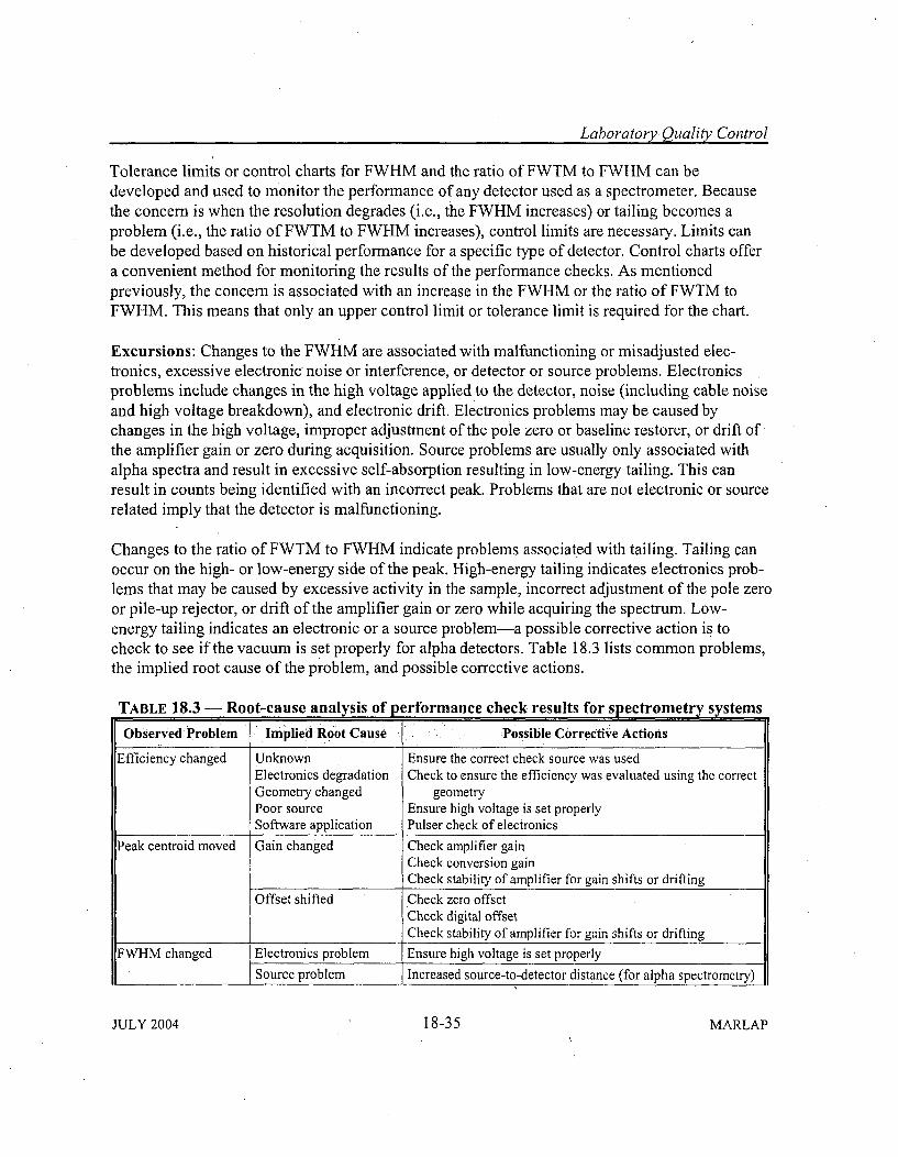
Laboratory Quality Control

Tolerance limits or control charts for FWHM and the ratio of FWTM to FWHM can bedeveloped and used to monitor the performance of any detector used as a spectrometer. Becausethe concern is when the resolution degrades (i.e., the FWHM increases) or tailing becomes aproblem (i.e., the ratio of FWTM to FWHM increases), control limits are necessary. Limits canbe developed based on historical performance for a specific type of detector. Control charts offera convenient method for monitoring the results of the performance checks. As mentionedpreviously, the concern is associated with an increase in the FWHM or the ratio of FWTM toFWHM. This means that only an upper control limit or tolerance limit is required for the chart.

Excursions: Changes to the FWHM are associated with malfunctioning or misadjusted elec-tronics, excessive electronic, noise or interference, or detector or source problems. Electronicsproblems include changes in the high voltage applied to the detector, noise (including cable noiseand high voltage breakdown), and electronic drift. Electronics problems may be caused bychanges in the high voltage, improper adjustment of the pole zero or baseline restorer, or drift ofthe amplifier gain or zero during acquisition. Source problems are usually only associated withalpha spectra and result in excessive self-absorption resulting in low-energy tailing. This canresult in counts being identified with an incorrect peak. Problems that are not electronic or sourcerelated imply that the detector is malfunctioning.

Changes to the ratio of FWTM to FWHM indicate problems associated with tailing. Tailing canoccur on the high- or low-energy side of the peak. High-energy tailing indicates electronics prob-lems that may be caused by excessive activity in the sample, incorrect adjustment of the pole zeroor pile-up rejector, or drift of the amplifier gain or zero while acquiring the spectrum. Low-energy tailing indicates an electronic or a source problem-a possible corrective action is tocheck to see if the vacuum is set properly for alpha detectors. Table 18.3 lists common problems,the implied root cause of the problem, and possible corrective actions.

TABLE 18.3 - Root-cause analysis of performance check results for spectrometry systems

Observed Problem Implied Root Cause Possible Corrective Actions

Efficiency changed Unknown Ensure the correct check source was usedElectronics degradation Check to ensure the efficiency was evaluated using the correctGeometry changed geometryPoor source Ensure high voltage is set properlySoftware application Pulser check of electronics

Peak centroid moved Gain changed Check amplifier gainCheck conversion gainCheck stability of amplifier for gain shifts or drifting

Offset shifted Check zero offsetCheckdigital offsetCheck stability of amplifier for gain shifts or drifting

FWHM changed Electronics problem Ensure high voltage is set properlySource problem Increased source-to-detector distance (for alpha spectrometry)

JULY 2004 18-35 MARLAP

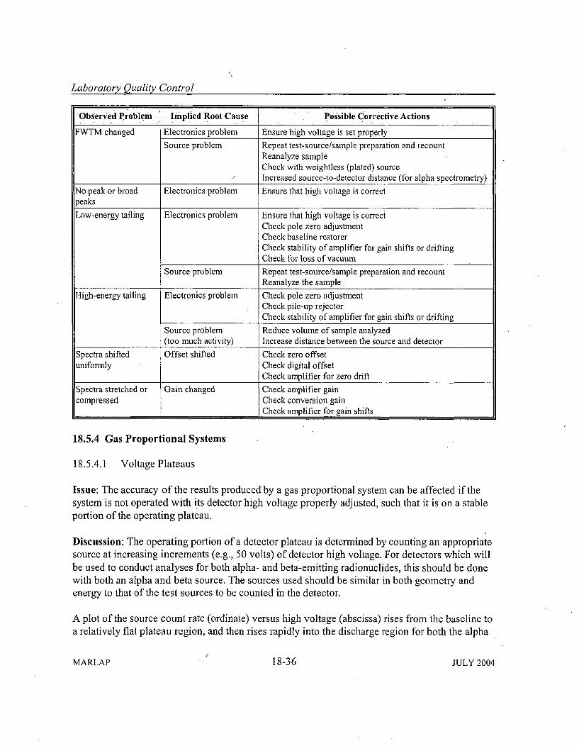
Laboratory Quality Control

Observed Problem Implied Root Cause Possible Corrective Actions

FWTM changed Electronics problem Ensure high voltage is set properly

Source problem Repeat test-source/sample preparation and recountReanalyze sampleCheck with weightless (plated) sourceIncreased source-to-detector distance (for alpha spectrometry)

No peak or broad Electronics problem Ensure that high voltage is correctpeaksLow-energy tailing Electronics problem Ensure that high voltage is correct

Check pole zero adjustmentCheck baseline restorerCheck stability of amplifier for gain shifts or driftingCheck for loss of vacuum

Source problem Repeat test-source/sample preparation and recountReanalyze the sample

High-energy tailing Electronics problem Check pole zero adjustmentCheck pile-up rejector

_ Check stability of amplifier for gain shifts or drifting

Source problem Reduce volume of sample analyzed(too much activity) Increase distance between the source and detector

Spectra shifted Offset shifted Check zero offsetuniformly Check digital offset

Check amplifier for zero driftSpectra stretched or Gain changed Check amplifier gaincompressed Check conversion gain

Check amplifier for gain shifts

18.5.4 Gas Proportional Systems

18.5.4.1 Voltage Plateaus

Issue: The accuracy of the results produced by a gas proportional system can be affected if thesystem is not operated with its detector high voltage properly adjusted, such that it is on a stableportion of the operating plateau.

Discussion: The operating portion of a detector plateau is determined by counting an appropriatesource at increasing increments (e.g., 50 volts) of detector high voltage. For detectors which willbe used to conduct analyses for both alpha- and beta-emitting radionuclides, this should be donewith both an alpha and beta source. The sources used should be similar in both geometry andenergy to that of the test sources to be counted in the detector.

A plot of the source count rate (ordinate) versus high voltage (abscissa) rises from the baseline toa relatively flat plateau region, and then rises rapidly into the discharge region for both the alpha

MARLAP 18-36 JULY 2004

Laboratoty Quality Control

and beta determinations. From the plateau, the operating voltage is selected so that small voltagechanges will only result in minor fluctuations to detector efficiency. Operation of the counter atthe upper end of the plateau is not recommended and can result in the generation of spuriousdischarge counts. Modern high-voltage supplies, operating properly, experience little actualvoltage fluctuation. The detector response should be checked after repairs and after a change ofgas. The detector plateau should again be determined and plotted (voltage vs. count rate) afterrepairs, particularly to the detector unit.

The historical tracking of the establishment and maintenance of this operating parameter isrecommended; it aids in determining the probable cause of quality control failure and the identi-fication of long-term instrument deterioration. Items to be recorded include date/time, instrumentdetector designation, source number, check source response at the operating point, and pertinentinstrument parameters, such as lower level discriminator setting, alpha-discriminator setting,length of the plateau, operating high voltage setting, etc.

Excursions: Voltage changes of short- or long-term duration will affect reliability of a propor-tional counter. If the detector voltage is lowered sufficiently, there is a danger of operating belowthe plateau knee which, in effect, reduces the efficiency and would bias the results of any samplecount low. Should the voltage applied to the proportional detector be driven up to a point wherethe slope of the plateau is sufficiently great enough to increase the efficiency of the detector,sample counts may be biased high. A transient voltage increase of great enough magnitude couldintroduce spurious counts.

Shifts in the operating voltage along the plateau or length of the plateau could also result fromlong-term detector deterioration or electronic drift or failure.

18.5.4.2 Self-Absorption, Backscatter, and Crosstalk

Issue: The accuracy of alpha and beta activity determinations in samples with discernable solidsin a gas proportional system depends in large part on the determination and maintenance of self-absorption and crosstalk curves.

Discussion: Samples counted for alpha and beta activity in a gas proportional system are typi-cally prepared as inorganic salts, e.g., nitrates, carbonates, oxides, sulfates, or oxalates, andcontain on the order of tens to hundreds of milligrams of solids when counted, which result inabsorption and scattering of the particles in the sample material and mounting planchet (Chapter16). Thus, for gas proportional systems, the detection efficiency for a given test source dependson the self-absorption occurring within each sample volume/mass. To establish the correctionfactor, a calibration curve is generated using a series of calibration sources consisting of anincreasing amount of solids and known amounts of radionuclide. The relative efficiency for eachcalibration source is plotted against theamount of solids, and these data are used to determine a

JULY 2004 18-37 MARLAP

Laboratory Quality Control

test source's efficiency as a function of test-source mass. The diameter and the composition ofthe test-source planchet, not just the test-source mass, should be identical with what was used forroutine samples. This allows calculation of the corrected amount of activity regardless of the test-source mass (mass/efficiency curves).

The counting of alpha and beta particles simultaneously in a proportional counter requires that anelectronic discriminator be adjusted, such that pulses of heights below that represented by thediscriminator are registered as betas, and those of greater heights are counted as alphas. Crosstalkoccurs when alpha particles are counted in the beta channel or betas are registered as alphas.For example, the alpha-to-beta crosstalk for "4'Am, which also has a 59.5 keV gamma-rayemission (35.9 percent), would be greater than the alpha-to-beta crosstalk factor for a pure alphaemitter (such as 21"Po). However, this relationship is energy dependent, and care should be takento identify samples that differ significantly from the sources used to establish the crosstalk ratio.For example, 9°Sr + 90Y (Epmax 2.28 MeV) is typically used as a beta source for instrumentcalibration. However, samples containing natural uranium in equilibrium with its progenyproduce beta emissions that are considerably more energetic from the 3.28 MeV Epmax betas of214Bi. The crosstalk ratio established with 9°Sr will be inadequate for such samples.

As the amount of solids in the test source increases, the beta crosstalk can increase due to thedegradation of the alpha particle energy by interaction with test-source material. Similarly, thebeta into alpha crosstalk decreases. Thus, crosstalk should be evaluated as a function of sampleweight to correct the observed relative alpha and beta counts. This is normally determined inconjunction with the self-absorption curve. To check these parameters, calibration sources shouldbe prepared at the low and high ends of the calibration curve, and the limit of their acceptabilityshould be better than 1 percent (one sigma). These checks should be performed annually, at aminimum, and following detector replacement or significant repair. The historical tracking of theestablishment and maintenance of these operating parameters is recommended. This aids indetermining the probable cause of quality control failure and the identification of long-terminstrument deterioration. In addition, items to be recorded include date/time, instrument detectordesignation, source number, operating point, and pertinent instrument parameters, such as lowerlevel discriminator setting, alpha discriminator setting, etc.

Excursions: Any change in the detector-source geometry or adsorption characteristics betweenthe source and detector, can affect the self-absorption and crosstalk correction factors. Forexample, the replacement of a detector window with one whose density thickness is differentfrom the original window can necessitate the reestablishment of these parameters. Electronic driftof the alpha discriminator can also affect the crosstalk ratios.

18.5.5 Liquid Scintillation

Issue: The accuracy and reproducibility of radionuclide measurements by liquid scintillation are

MARLAP 18-38 JULY 2004

Laboratoiy Quality Control

dependent on accounting for the quench (Section 15.5.3.3) of the measured test source. Quenchis one of the most significant factors to be accounted for, and can be affected by solvent-to-fluorratio, cocktail characteristics, suspension composition, acid concentration, and chemical andradiological impurities. Care must be taken to assure radionuclide purity and chemical-composition equivalence to calibration and test sources. An additional factor to consider is theratio of sample volume to scintillation-cocktail volume (i.e., dilution factor). Although this canaffect quench as well (especially if there is significant sample dilution), it is more critical that theratios used for calibration match those in the test-source analysis.

Discussion: The process of scintillation involves the energy transfer from the emitted betaparticles, slowing and stopping in the liquid medium as a result of collisions with molecularlybound electrons. The transfer of energy from the beta particle to the electrons results in solventexcitation through thermal, collisional, and photonic interactions. These excited solventmolecules transfer energy through various processes to specific organic molecules known as"fluors." The combination of the solvent and fluor is referred to as the "cocktail." The test sourceis the combination of the cocktail and sample.

Fluors absorb the energy and are brought to an excited state. The de-excitation of these moleculesresults in a photon emission that is detected by a photomultiplier tube. Many cocktail combina-tions contain a second fluor (referred to as a wavelength shifter) which adjusts the emittedphotons to a specific bandwidth.

Any component of the cocktail that affects the energy transfer process will have a significanteffect on the analysis. This effect is referred to as "quench." The quench of a cocktail can beaffected by:

* Color;" Turbidity;" Molecules of high electron affinity;" Solvent;• Acidity; and" Dissolved gases.

Quench has the effect of shifting the energy distribution of the beta particle spectrum to lowerenergies. Quench also can have the effect of reducing the number of net counts.

Excursions: Slowly changing liquid scintillation measurements of a sample may be due to thechange in quench because of chemical attack on the cocktail system or to changes in instrumentor ambient temperature during a long count. Rapid changes in liquid scintillation measurementsinclude phase separation of the sample in the cocktail, sample precipitation, and light leaks intothe instrument. Some causes of excursions in liquid scintillation analysis are listed in Table 18.4.

JULY 2004 18-39 MARLAP

Laboratory Quality Control

Examples: Specific examples of these types of excursions as it affects analysis can be seen in theexamples below.

TABLE 18.4 - Some causes of excursions in liquid scintillation analysisPhysiOcalEffects .... ChemicalEffects

Turbidity Elevated concentrations of Cl or NO,

Sample opacity or color Solvents: CHCI3 , methyl ethyl ketone, CC14 , etc.

Precipitation Peroxide

Fingerprints on vial Incorrect fluor

Phase separation Expired fluor

Light leaks into instrument Contaminated fluor

Inadequate dark adaptation

Temperature changesDifferent vial composition

MEASUREMENT OF 55FE IN RADIOACTIVE WASTE SOLUTIONS. The separation techniques for irongenerally use nitric and hydrochloric acids. Both of these acids are eliminated prior to thepreparation of the cocktail by boiling down the solution with phosphoric acid. Nitric acid candecompose in room light giving rise to the gas N204 , which can impart a brown color to thesolution. High concentrations of chloride can act as electron scavengers in the solution. Boththese conditions yield quench. Removing them with phosphoric acid maintains the solutionacidity (so the iron does not precipitate) and does not act as a quench agent.

SAMPLES IN CONCENTRATED NITRIC ACID. If samples must be made with high concentrations ofnitric acid, they should be measured shortly after preparation, to avoid fluor decomposition. Thesamples need to have their quench compared to standard samples of the same acid compositionand short time following preparation.

TRITIUM IN RAINWATER. Some methods of collecting rainwater involve funneling from a largesurface area (like a roof) into a collection bottle through a spout. Rainwater itself contains manycontaminants, such as carbon dioxide, sulfur dioxide, and polycyclic aromatic hydrocarbons(PAHs from fossil fuel combustion), which can act as significant quench agents. Furthermore,the surface through which the water is collected may contain accumulated particulate matter thatalso can affect the quench. Distilling the sample would minimize the effect of their quench.Without this, the quench would be increased and the "apparent" value would have a significantuncertainty associated with it.

18.5.6 Summary Guidance on Instrument Calibration, Background, and Quality Control

Radiation detectors and nuclear instrumentation, such as spectrometry systems, should be

MARLAP 18-40 JULY 2004

Laboratory Quality Control

calibrated and maintained according to protocols and procedures documented in the laboratory'sstandard operating procedures and quality manual. The important calibration parameters, theperformance criteria used to monitor these calibration parameters, and the frequency of re-calibrations should be addressed in these documents. Another important parameter that should beaddressed is the detector background. Detector background measurements should be taken at anappropriate frequency for the purposes of determining the net count rate of a test source and forcontrolling contamination.

The following subsections discuss the important calibration and monitoring parametersassociated with nuclear instrumentation in common use at radioanalytical laboratories. At the endof each subsection, a table provides some examples of performance criteria for the measurementparameters and the frequency of monitoring of these parameters. The information in thesesubsections conforms to ASTM E181, ANSI N42.12, and NELAC (2002) and uses the input ofthe ASTM D19.04 Subcommittee on Methods of Radiochemical Analyses for Radioactivity inWater. A few important concepts should be considered when reviewing the following sectionsand summary Tables 18.5 through 18.8:

" NIST-traceable radionuclide sources (or traceable to a national standards body) are to be usedfor all calibrations when possible (see Chapter 15, Quantification of Radionuclides). Sourcesused for QC checks do not have to be NIST-traceable.

" The frequency of performing QC detector-response measurements, or evaluating a detectorbackground, is related to the risk (probability) that a laboratory will accept for not detectingan instrument problem or a change in background, given a certain number of samplesanalyzed. The acceptable risk for not detecting a problem may vary from one laboratory toanother. If an instrument QC response check is performed once every 10 samples (testsources), then there is a possibility that nine samples may be counted on an instrument notmeeting quality specifications before a problem is detected. Therefore, it is more appropriateto establish the frequency of instrument QC based on the number of samples processed ratherthan on time schedules. The examples of instrument QC frequencies presented in thefollowing sections are considered practical for most laboratories.

* Loss of control results from a calibration performance criterion not beingmet, any repair ormaintenance that could affect a.calibration parameter, and any event (such as sudden loss ofpower) that could affect calibration.

" Even without loss of control, a counting or spectrometry system should be re-calibrated fortest-source radionuclides, matrices, and counting geometries at a frequency consistent withspecifications delineated in the laboratory's quality manual.

" For an accurate measurement of a detector's counting efficiency and resolution, as well as fora detector's QC response checks, the relative counting uncertainty (I a) of the measurement(net count or net response) or in the individual peaks associated with spectrometry systems

JULY 2004 18-41 MARLAP

Laboratoi-y Quality Control

should be 1 percent or less.

Detector background measurements are used for the calculation of a net measurementresponse and for detector contamination control. A net measurement response is calculatedusing a long-duration detector background measurement in order to minimize the countinguncertainty of the measurement. Contamination control background measurements typicallyare taken more frequently and are of shorter duration than those for net measurementresponse applications. To determine possible gross contamination, the results from thecontamination control background measurements should be evaluated statistically andcompared to the long-duration background results.

18.5.6.1 Gas Proportional Counting Systems

CALIBRATIONS

Three parameters should be considered when calibrating a gas proportional counting system:

* Operating voltage settings on the alpha andbeta voltage plateaus,* Detector counting efficiencies, and" Crosstalk factors.

Initially upon instrument setup, the manufacturer's specifications for these three parametersshould be verified. It shouldbe noted that the manufacturer's specifications may be based uponunique calibration sources and operating conditions that may not be similar to those used whenanalyzing test sources. For example, the manufacturer's detector efficiency and crosstalk factorsmay be based on electroplated alpha and beta sources. For most laboratories, the typical testsource for GP counting is not an electroplated source, so the reference alpha and beta radio-nuclides for calibration are not the same as the radionuclides used by the manufacturer indeveloping the specifications. However, the detector's alpha and beta voltage plateau settingstypically are not changed after instrument setup. The alpha and beta voltage plateau settings areselected from plots of the applied detector voltage versus the observed count rate for pure alphaand beta sources (see Chapter 15, Quantification ofRadionuclides).

The next parameters to evaluate are the detector's alpha and beta counting efficiencies forvarious source geometries. Initially, the manufacturer's detector efficiency for both alpha andbeta counting modes should be verified using electroplated sources. (Typical electroplatedcalibration sources include 99Tc and 9"Sr for beta sources and 23°Th or "4'Am for alpha sources.) Adetector's counting efficiency should be determined for each radionuclide and method used toanalyze test sources. The detector efficiency should be determined for new or changed methodprotocols and loss of instrument control. For test sources having mass loading, an efficiencycurve or mathematical function that describes the detector efficiency versus mass loading,consistent with the expected test source mass range, should be developed. For any mass in the

MARLAP 18-42 JULY 2004

Laboratory Quality Control

expected calibration range, the 95-percent confidence limits for the detection efficiency shouldbe within 10 percent of the fitted value for alpha sources and within 5 percent of the fitted valuefor beta sources.

The crosstalk factors for the alpha counts into the beta channel (alpha crosstalk) and for the betacounts in the alpha channel (beta crosstalk) should be determined when applicable. Themanufacturer's specifications for the crosstalk factors using electroplated sources should beverified prior to test source processing. Typical manufacturer specifications for electroplatedsources are less than 1 percent alpha counts in the beta channel for 2 1"Po and less than 0.1percent beta counts in the alpha channel for 90Sr/Y. The alpha crosstalk factor will vary accordingto the crosstalk parameter setup, decay scheme of the alpha emitting radionuclide, and the mass(weight) of the source. Verify the manufacturer's alpha crosstalk factor using the radionuclideand crosstalk parameters setting specified by the manufacturer. The alpha crosstalk factor forother radionuclides and source masses should be determined for each method, preferably at thesame time as determining the detector counting efficiency factors or efficiency versus sourcemass function. The crosstalk factors may be method specific and should be determined duringinitial calibration and after re-calibrations.

BACKGROUND

A detector's background should be determined immediately after calibration and at the instru-ment settings established for each method. An accurate estimate of a detector's background isneeded to determine the net count rate of a source. For this application, a very long background,with respect to the nominal counting time for the test sources, typically is needed depending'onthe required detection limit. One approach for making long-duration background measurementsis to count a clean test-source mount long enough to achieve a relative counting uncertainty (1 a)of less than 10 percent for alpha measurements and less than 3 percent for beta measurements.Alternatively, the counting time for a long-duration background measurement should be betweenone and four times the nominal counting duration of test sources for a given matrix andapplication. A long-duration background measurement should be conducted on a monthly basis.A statistical test should be used to determine if the detector's background has changed from theinitial background determination.

When required, a detector may be evaluated frequently for gross contamination using a short-duration counting interval. When the counting duration of test sources is short (less than onehour), a short-duration background measurement should be conducted prior to processing testsources. When the test-source counting time is longer, the background time interval should be thesame as the test sources, and the background should be determined before and after a sample (testsource) batch.

CALIBRATION QC CHECKS

JULY 2004 18-43 MARLAP

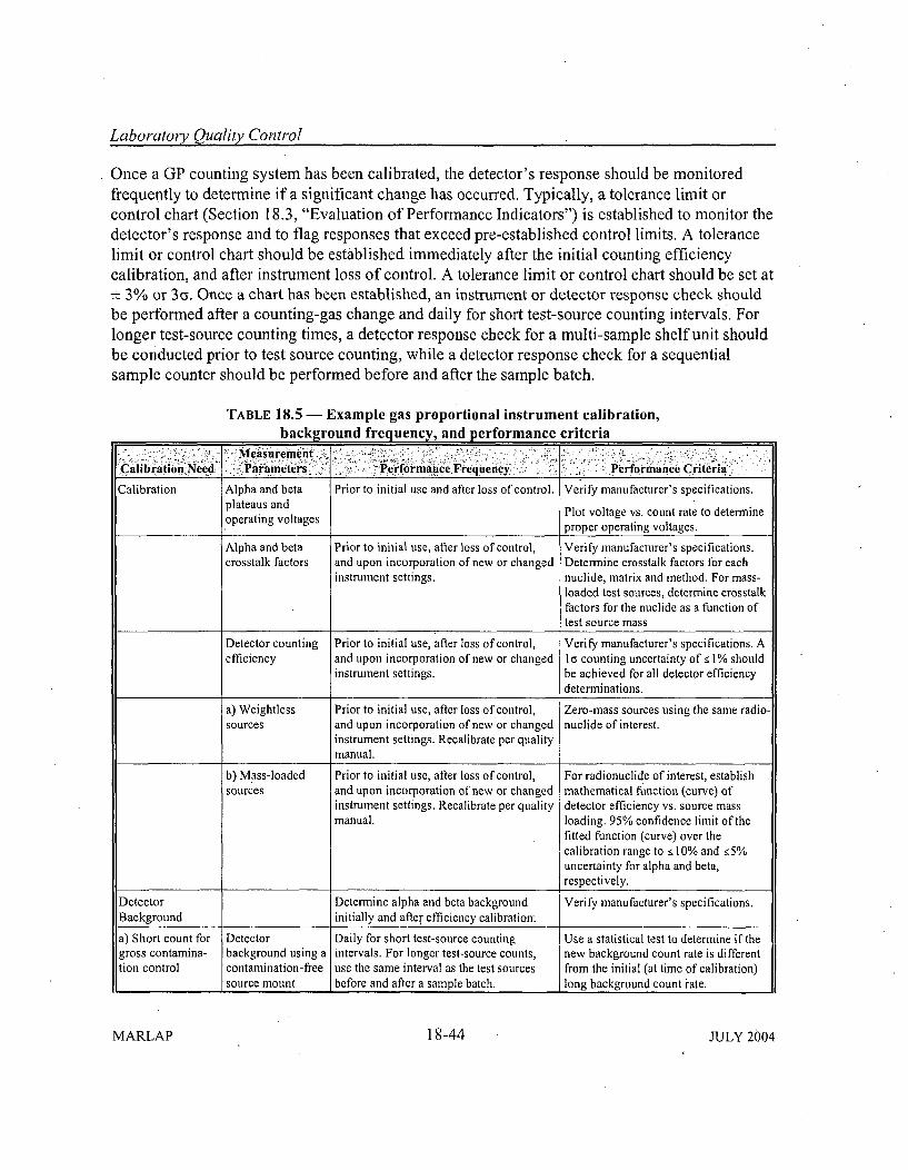
Laboratory Quality Control

Once a GP counting system has been calibrated, the detector's response should be monitoredfrequently to determine if a significant change has occurred. Typically, a tolerance limit orcontrol chart (Section 18.3, "Evaluation of Performance Indicators") is established to monitor thedetector's response and to flag responses that exceed pre-established control limits. A tolerancelimit or control chart should be established immediately after the initial counting efficiencycalibration, and after instrument loss of control. A tolerance limit or control chart should be set at± 3% or 3R. Once a chart has been established, an instrument or detector response check shouldbe performed after a counting-gas change and daily for short test-source counting intervals. Forlonger test-source counting times, a detector response check for a multi-sample shelf unit shouldbe conducted prior to test source counting, while a detector response check for a sequentialsample counter should be performed before and after the sample batch.

TABLE 18.5 - Example gas proportional instrument calibration,background frequency, and performance criteria

~Mea'sureffent: .--

Calibratio nNeed Parameters .Performance Frequency Performance Criteria

Calibration Alpha and beta Prior to initial use and after loss of control. Verify manufacturer's specifications.plateaus andoperating voltages Plot voltage vs. count rate to determine

proper operating voltages.

Alpha and beta Prior to initial use, after loss of control, Verify manufacturer's specifications.crosstalk factors and upon incorporation of new or changed Determine crosstalk factors for each

instrument settings. nuclide, matrix and method. For mass-loaded test sources, determine crosstalkfactors for the nuclide as a function oftest source mass

Detector counting Prior to initial use, after loss of control, Verify manufacturer's specifications. Aefficiency and upon incorporation of new or changed I a counting uncertainty of-• 1% should

instrument settings. be achieved for all detector efficiencydeterminations.

a) Weightless Prior to initial use, after loss of control, Zero-mass sources using the same radio-sources and upon incorporation of new or changed nuclide of interest.

instrument settings. Recalibrate per qualitymanual.

b) Mass-loaded Prior to initial use, after loss of control, For radionuclide of interest, establishsources and upon incorporation of new or changed mathematical function (curve) of

instrument settings. Recalibrate per quality detector efficiency vs. source massmanual. loading. 95% confidence limit of the

fitted function (curve) over thecalibration range to •10% and g 5%uncertainty for alpha and beta,respectively.

Detector Determine alpha and beta background Verify manufacturer's specifications.Background initially and after efficiency calibration.

a) Short count for Detector Daily for short test-source counting Use a statistical test to determine if thegross contamina- background using a intervals. For longer test-source counts, new background count rate is differenttion control contamination-free use the same interval as the test sources from the initial (at time of calibration)

source mount before and after a sample batch, long background count rate.

MARLAP 18-44 JULY 2004

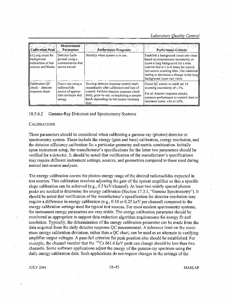
Laboratory Quality Control

Measur.ementCalibration Neetid, Parameters PerformanceeFrequency Performance Criteria

b) Long count for Detector back- Monthly when system is in use. Establish a background count rate valuebackground ground using a based on measurement uncertainty orsubtraction of test contamination-free count a long background for a timesources and blanks source mount interval that is I to 4 times the typical

test-source counting time. Use statisticaltesting to determine a change in the longbackground count rate value.

Calibration QC Count rate using a Develop detector response control chart Count QC source to reach net I acheck - detector radionuclide immediately after calibration and loss of counting uncertainty of <•1%.response check source of approp- control. Perform detector response check

riate emission and daily, prior-to-use, or bracketing a sample For all detector response checks,

energy batch depending on test source counting compare performance to control chart or

time. I tolerance limits: ±3a or -3%.

18.5.6.2 Gamma-Ray Detectors and Spectrometry Systems

CALIBRATIONS

Three parameters should be considered when calibrating a gamma-ray (photon) detector orspectrometry system. These include the energy (gain and base) calibration, energy resolution, andthe detector efficiency calibration for a particular geometry and matrix combination. Initiallyupon instrument setup, the manufacturer's specifications for the latter two parameters should beverified for a detector. It should be noted that verification of the manufacturer's specificationsmay require different instrument settings, sources, and geometries compared to those used duringnormal test-source analyses.

The energy calibration covers the photon energy range of the desired radionuclides expected intest sources. This calibration involves adjusting the gain of the system amplifier so that a specificslope calibration can be achieved (e.g., 0.5 keV/channel). At least two widely spaced photonpeaks are needed to determine the energy calibration (Section 17.3.1, "Gamma Spectrometry"). Itshould be noted that verification of the manufacturer's specification for detector resolution mayrequire a difference in energy calibration (e.g., 0. 10 or 0.25 keV per channel) compared to theenergy calibration settings used for typical test sources. For most modem spectrometry systems,the instrument energy parameters are very stable. The energy calibration parameter should bemonitored as appropriate to support data-reduction algorithm requirements for energy fit andresolution. Typically,. the determination of the energy calibration parameter can be made from thedata acquired from the daily detector response QC measurement. A tolerance limit on the maxi-mum energy calibration deviation, rather than a QC chart, can be used as an alternate to verifyingamplifier output voltages. A pass-fail criterion for peak position also should be established. Forexample, the channel number that the "37Cs 661.6 keV peak can change should be less than twochannels. Some software applications adjust the energy of the gamma-ray spectrum using thedaily energy calibration data. Such applications do not require changes in the settings of the

JULY 2004 18-45 MARLAP

Laboratory Quality Control

system's electronics.

The manufacturer's detector resolution, expressed as the FWHM inkeV at specific photonenergies, should be verified prior to use. Manufacturers of detector systems routinely establish anenergy calibration of 0.25 or 0.10 keV/channel by adjusting the gain of the detection systemamplifier. The FWHM and the peak-to-Compton ratio are both measured at a specified distancefrom the detector. Analytical laboratories frequently calibrate energies at approximately 0.50keV/channel. Thus, prior to initial calibration or when re-calibration is necessary, the analyticallaboratory should duplicate the manufacturers conditions for FWHM and peak-to-Compton ratioat the manufacturers stated initial conditions for the detector. It should be noted that the detectorresolution varies with energy (Chapter 15) and can be affected by such factors as temperature,humidity, vibration, poor connectors, or poor line-voltage conditioning. The QC check sourcesused for the detector response check typically are used for resolution measurements during test-sources analyses. For a combined detector response and resolution check, the radionuclidesselected for the QC source have photon energies that normally cover the low, middle, and highenergies of the desired range (e.g., 24"Am, '37Cs, and 6"Co). The photon energies selected for theresolution check should be sufficiently separated to avoid other interfering peaks. If the energycalibration settings for routine test source analyses is 0.5 keV per channel or greater, a resolutioncheck may only indicate gross or substantial changes in a detector's resolution (e.g., greater than10 to 20 percent). Photopeaks with greater than 10,000 counts are needed for routine resolutionchecks. Once the routine (operational) resolution value has been determined, limiting the maxi-mum resolution deviation with an acceptable tolerance limit may be more suitable than using aQC chart. QC verification of resolution should be performed on a pass-fail basis. Since theFWHM varies as a function of energy, each peak should have its own acceptance criterion.

The peak-to-Compton ratio is an important characteristic of the detector that needs to becompared with the manufacturers specification upon initial detector calibration. This ensures thatthe maximum sensitivity for full energy peak (FEP) analysis is achieved, and the correctsemiconductor crystal has been installed in'the detector housing. See Section 15.6.2.1, "DetectorRequirements and Characteristics," for the definition and technical basis for the peak-to-Compton ratio determination. This parameter needs to be checked during initial detector setup orprior to detector recalibration.

The next parameter that should be evaluated is the detector's efficiency response as a function ofenergy and matrix. The manufacturer's specification for detector efficiency is relative theefficiency of a 76 x 76 mm Nal detector responding to to 57Co, 137Cs, and 6°Co point sources at adistance of 25 cm from the detector. The standard Nal efficiency for this detector size and a 6"Copoint source is 0.1 percent. (Gilmore and Hemingway, 1995). For each geometry/matrixcombination used for test-source analyses, a gamma-ray efficiency versus energy responsefunction (curve) must be determined. It is important that the same geometry and matrix be usedfor the calibration and test sources. This includes the container for these sources, as well as theirphysical placement relative to the detector. The efficiency check should span the energy range of

MARLAP 18-46 JULY 2004

Laboratory Quality Control

radionuclides of interest. For commercially available mixed radionuclide calibration sources, 10data points per calibration curve is typical, covering the range of 59 keV (241Am) to 1,836 (88Y)keV. The 95 percent confidence limit of the fitted curve should be under 8 percent over thecalibration energy region. A detector response QC chart should be established immediately afterthe first calibration for the detector.

DETECTOR BACKGROUND

A detector's background should be determined immediately after calibration with or without acounting container, depending on the inherent radionuclide activity levels in the countingcontainer. An accurate estimate of a detector's background in a radionuclide photopeak is neededwhen determining the net photopeak count rate of a source. For this application, a very longbackground with respect to the nominal counting time for the test sources typically is needed,depending on the required detection limit. One approach for making long-duration backgroundmeasurements is to count a clean test source mount to achieve a relative counting uncertainty(la) for major photopeaks that is < 10 percent. Alternatively, the counting interval for the longcount should be between one and four times the nominal counting interval of the test sources. Along detector background measurement should be conducted on a monthly or quarterly basis. Astatistical test should be used to determine if the detector background in a photopeak has changedsignificantly from the initial background determination. Acceptable integrated background valueswill be defined by the measurement limits desired by the analytical method. The statisticalcriterion that constitutes a significant change should be stated in the laboratory's quality manual.

When required, the detector's background may be evaluated for gross contamination on afrequent basis using a short counting interval. Once the long background count rate has beendetermined, a shorter background count can be made and the results compared statistically to thelong background count rate to determine possible detector contamination. For the short back-ground, the energy region between about 50 and 2,000 keV is integrated. The counting time forthe short background count should be set so that the relative counting uncertainty (1 a) of theintegrated counts is -•3 percent. A limit in the deviation of the integrated background value maybe set using a tolerance limit or control chart. It should be verified that no extraneous peaks areidentified, indicating lower-level contamination (i.e., no new peaks in the short backgroundspectrum compared to previous spectra)

CALIBRATION QC CHECKS

After the initial detector calibration, a control chart or tolerance limit should be established(Section 18.3, "Evaluation of Performance Indicators"). Such a chart may be generated using anoncalibrated, but reproducible geometry. This source does not necessarily need to be a primary-grade calibration source, but a sealed source that is well characterized and stable. The purpose ofthis QC source is to validate that the detector performance is reproducible on a day-to-day basisfor the detector efficiency, energy response, and resolution. These characteristics can be used on

JULY 2004 18-47 MARLAP

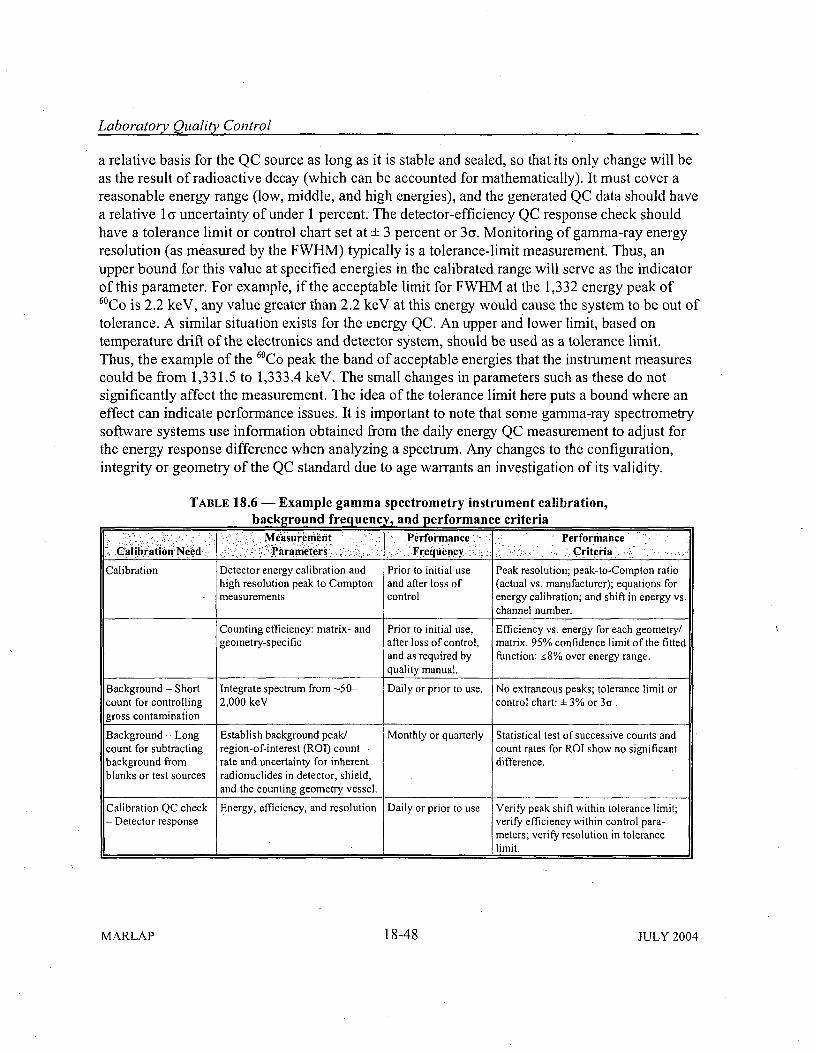
Laboratory Quality Control

a relative basis for the QC source as long as it is stable and sealed, so that its only change will beas the result of radioactive decay (which can be accounted for mathematically). It must cover areasonable energy range (low, middle, and high energies), and the generated QC data should havea relative 1 a uncertainty of under 1 percent. The detector-efficiency QC response check shouldhave a tolerance limit or control chart set at ± 3 percent or 3a. Monitoring of gamma-ray energyresolution (as measured by the FWHM) typically is a tolerance-limit measurement. Thus, anupper bound for this value at specified energies in the calibrated range will serve as the indicatorof this parameter. For example, if the acceptable limit for FWHM at the 1,332 energy peak of"°Co is 2.2 keV, any value greater than 2.2 keV at this energy would cause the system to be out oftolerance. A similar situation exists for the energy QC. An upper and lower limit, based ontemperature drift of the electronics and detector system, should be used as a tolerance limit.Thus, the example of the 6"Co peak the band of acceptable energies that the instrument measurescould be from 1,331.5 to 1,333.4 keV. The small changes in parameters such as these do notsignificantly affect the measurement. The idea of the tolerance limit here puts a bound where aneffect can indicate performance issues. It is important to note that some gamma-ray spectrometrysoftware systems use information obtained from the daily energy QC measurement to adjust forthe energy response difference when analyzing a spectrum. Any changes to the configuration,integrity or geometry of the QC standard due to age warrants an investigation of its validity.

TABLE 18.6 - Example gamma spectrometry instrument calibration,background frequency, and performance criteria

asu.rement . . Performance ., Performance.,.Calibration Need, .arameters . Frqec ... . Criteria'

Calibration Detector energy calibration and Prior to initial use Peak resolution; peak-to-Compton ratiohigh resolution peak to Compton and after loss of (actual vs. manufacturer); equations for

- measurements control energy calibration; and shift in energy vs.channel number.

Counting efficiency: matrix- and Prior to initial use, Efficiency vs. energy for each geometry/geometry-specific after loss of control, matrix. 95% confidence limit of the fitted

and as required by function: •8% over energy range.quality manual.

Background - Short Integrate spectrum from -50- Daily or prior to use. No extraneous peaks; tolerance limit orcount for controlling 2,000 keV control chart: ± 3% or 3o.gross contamination

Background - Long Establish background peak/ Monthly or quarterly Statistical test of successive counts andcount for subtracting region-of-interest (ROI) count count rates for ROI show no significantbackground from rate and uncertainty for inherent difference.blanks or test sources radionuclides in detector, shield,

and the counting geometry vessel.

Calibration QC check Energy, efficiency, and resolution Daily or prior to use Verify peak shift within tolerance limit;- Detector response verify efficiency within control para-

meters; verify resolution in tolerance_ limit.

MARLAP 18-48 JULY 2004

Laboratory Quality Control

18.5.6.3 Alpha Detector and Spectrometry Systems

CALIBRATIONS

Three parameters should be considered when calibrating an alpha detector or spectrometrysystem. These include the energy (gain and base) calibration, energy resolution, and the detectorefficiency for a particular combination of geometry and matrix. Additionally, a detector's leakagecurrent typically is monitored to detect detector problems and possible detector-chamber lightleaks. The manufacturer's specifications for detector resolution and efficiency should be verifiedinitially upon instrument setup. Verifying the manufacturer's specifications may require differentinstrument settings and sources compared to those used during normal test-source analyses. Theinstrument setup and source geometry details normally are included in the manufacturer'sdocumentation for a semiconductor alpha detector. The manufacturer's detector resolution(FWHM) in MeV is measured using an electroplated 24.Am point source in a near vacuum.

The energy calibration should be applicable to the alpha energies of the radionuclides expected inthe test sources. This calibration involves adjusting the gain of the system amplifier so that aspecific energy slope calibration can be achieved to cover a desired energy range. A typicalenergy range is between 3 and 8 MeV for long-lived radionuclides and between 3 and 10 MeVfor short-lived radionuclides. At least two widely spaced alpha peaks are needed to determine theenergy calibration. An energy calibration should be a linear response. However, the acceptabledeviation in the energy gain (MeV per channel) depends on the total number of channels and therange of the energy spectrum.

A detector's peak counting efficiency should be determined for each test-source geometry/matrixcombination that will be used. Calibration source mounts should be equivalent to the test-sourcemount (electroplated or microprecipitate) and have the radionuclide of interest or a radionuclidewith about the same alpha energy. Most radioanalytical methods using alpha spectrometryincorporate a radioisotope tracer (radiotracer) into the sample processing scheme as a means todetermine the sample-specific, chemical-yield detector-efficiency factor. For these methods, aseparate detector efficiency calibration is not needed. When radiotracers are not used to deter-mine the chemical-yield-to-detector efficiency factor, a detector should be calibrated for eachtest-source mounting geometry according to the frequency specified in the laboratory's qualitymanual For this calibration, the peak efficiency should be determined using the average of atleast two alpha peaks. When measuring a detector's counting efficiency, the source should becounted sufficiently long so that the relative uncertainty. (1r) of the alpha peak(s) count is •<3 toi• 1 percent.

DETECTOR BACKGROUND

A detector's background should be determined immediately after detector installation, instrumentsetup, detector calibration, or loss of control. The background counts in an alpha peak or a regionof interest for the expected radionuclides should be integrated. A blank test source mount (filter

JULY 2004 18-49 MARLAP

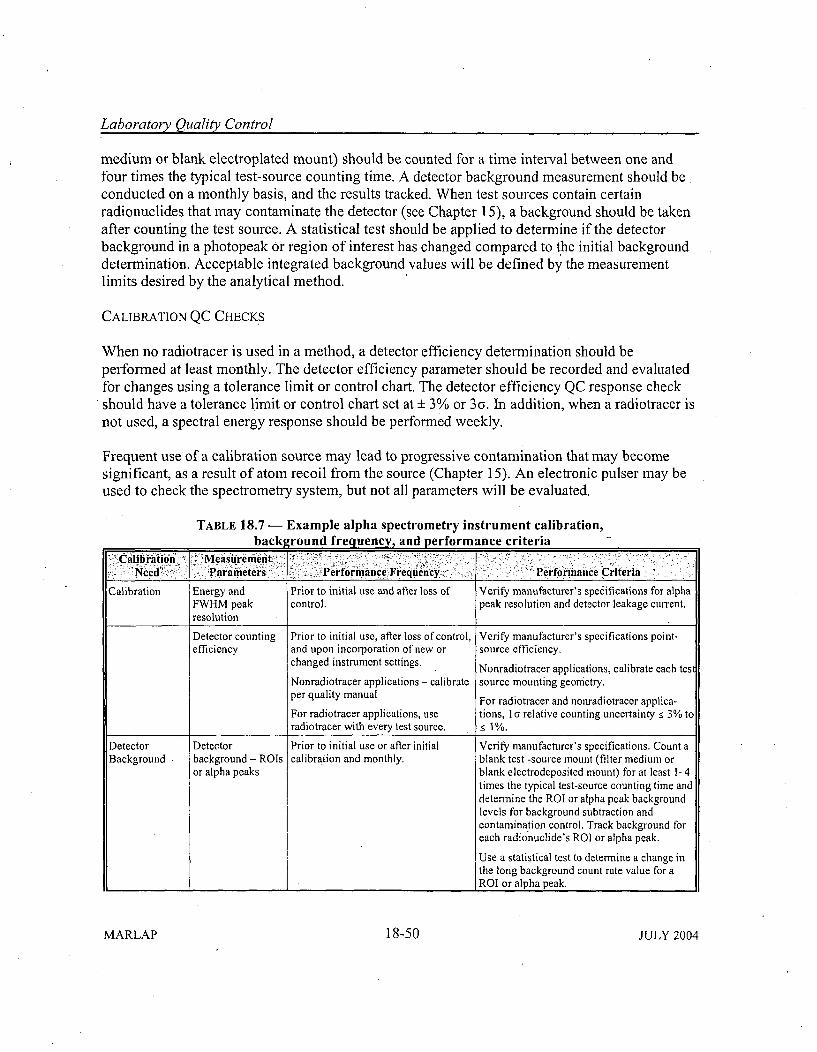
Laboratoty Quality Control

medium or blank electroplated mount) should be counted for a time interval between one andfour times the typical test-source counting time. A detector background measurement should beconducted on a monthly basis, and the results tracked. When test sources contain certainradionuclides that may contaminate the detector (see Chapter 15), a background should be takenafter counting the test source. A statistical test should be applied to determine if the detectorbackground in a photopeak or region of interest has changed compared to the initial backgrounddetermination. Acceptable integrated background values will be defined by the measurementlimits desired by the analytical method.

CALIBRATION QC CHECKS

When no radiotracer is used in a method, a detector efficiency determination should beperformed at least monthly. The detector efficiency parameter should be recorded and evaluatedfor changes using a tolerance limit or control chart. The detector efficiency QC response checkshould have a tolerance limit or control chart set at + 3% or 3y. In addition, when a radiotracer isnot used, a spectral energy response should be performed weekly.

Frequent use of a calibration source may lead to progressive contamination that may becomesignificant, as a result of atom recoil from the source (Chapter 15). An electronic pulser may beused to check the spectrometry system, but not all parameters will be evaluated.

TABLE 18.7 - Example alpha spectrometry instrument calibration,background frequency, and performance criteria

- Calibriation <, Measu-remniit, C Perrmance i teriaNeed ~Parameters Performance Frequency PromneCiei

Calibration Energy and Prior to initial use and after loss of Verify manufacturer's specifications for alphaFWI-HM peak control, peak resolution and detector leakage current.resolution

Detector counting Prior to initial use, after loss of control, Verify manufacturer's specifications point-efficiency and upon incorporation of new or source efficiency.

changed instrument settings. Nonradiotracer applications, calibrate each test

Nonradiotracer applications - calibrate source mounting geometry.per quality manual For radiotracer and nonradiotracer applica-

For radiotracer applications, use tions, 1 a relative counting uncertainty • 3% toradiotracer with every test source. • 1%.

Detector Detector Prior to initial use or after initial Verify manufacturer's specifications. Count aBackground background - ROls calibration and monthly. blank test -source mount (filter medium or

or alpha peaks blank electrodeposited mount) for at least 1-4times the typical test-source counting time anddetermine the ROI or alpha peak backgroundlevels for background subtraction andcontamination control. Track background foreach radionuclide's ROI or alpha peak.

Use a statistical test to determine a change inthe long background count rate value for aROI or alpha peak.

MARLAP 18-50 JULY 2004

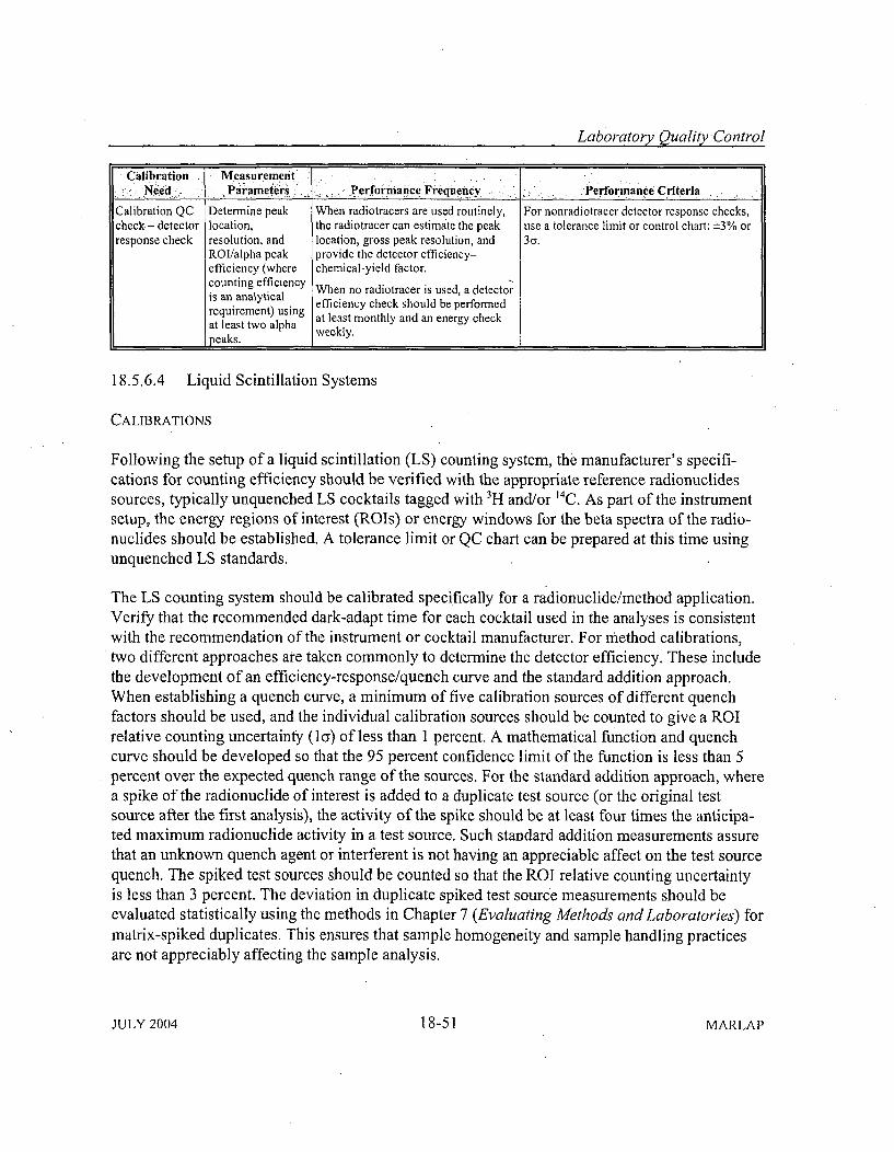
Laboratory Quality Control

Calibration Measurement'Need-,, Parameters , Performance Frequency Performance Criteria

Calibration QC Determine peak When radiotracers are used routinely, For nonradiotracer detector response checks,check- detector location, the radiotracer can estimate the peak use a tolerance limit or control chart: ±3% orresponse check resolution, and location, gross peak resolution, and 3o.

ROI/alpha peak provide the detector efficiency-efficiency (where chemical-yield factor.counting efficiency When no radiotracer is used, a detectoris an analytical efficiency check should be performedrequirement) using at least monthly and an energy checkat least two alpha week ly,peaks. weekly.

18.5.6.4 Liquid Scintillation Systems

CALIBRATIONS

Following the setup of a liquid scintillation (LS) counting system, the manufacturer's specifi-cations for counting efficiency should be verified with the appropriate reference radionuclidessources, typically unquenched LS cocktails tagged with 3H and/or 4̀C. As part of the instrumentsetup, the energy regions of interest (ROIs) or energy windows for the beta spectra of the radio-nuclides should be established. A tolerance limit or QC chart can be prepared at this time usingunquenched LS standards.

The LS counting system should be calibrated specifically for a radionuclide/method application.Verify that the recommended dark-adapt time for each cocktail used in the analyses is consistentwith the recommendation of the instrument or cocktail manufacturer. For method calibrations,two different approaches are taken commonly to determine the detector efficiency. These includethe development of an efficiency-response/quench curve and the standard addition approach.When establishing a quench curve, a minimum of five calibration sources of different quenchfactors should be used, and the individual calibration sources should be counted to give a ROIrelative counting uncertainty (Icy) of less than 1 percent. A mathematical function and quenchcurve should be developed so that the 95 percent confidence limit of the function is less than 5percent over the expected quench range of the sources. For the standard addition approach, wherea spike of the radionuclide of interest is added to a duplicate test source (or the original testsource after the first analysis), the activity of the spike should be at least four times the anticipa-ted maximum radionuclide activity in a test source. Such standard addition measurements assurethat an unknown quench agent or interferent is not having an appreciable affect on the test sourcequench. The spiked test sources should be counted so that the ROI relative counting uncertaintyis less than 3 percent. The deviation in duplicate spiked test source measurements should beevaluated statistically using the methods in Chapter 7 (Evaluating Methods and Laboratories) formatrix-spiked duplicates. This ensures that sample homogeneity and sample handling practicesare not appreciably affecting the sample analysis.

JULY 2004 18-51 MARLAP

Laboratoty Quality Control

INSTRUMENT BACKGROUND AND METHOD BLANKS

For methods that have quenched test sources, a quenched method blank (or mdan of severalquenched blanks) should be used to determine the background count rate that is subtracted fromthe count rate of the quenched test sources in a batch. A method background is determined bycounting a blank sample that has been taken through the analytical process for the radionuclide ofinterest and determining its quench. When prepared in this manner, the blank will have a quenchvalue similar to that of the test sources in the batch having the approximately the same quenchfactor. The counting interval of the blank should be the same or longer than the counting intervalof test sources in the batch. Multiple quenched blank measurements should be made to establisha mean quenched-background value and standard uncertainty of the mean (standard error of themean). These parameters should be used to determine the net count rate (and combined standarduncertainty) of test sources within a batch of samples. The ROI count rate of the quenched blanktest source (processed with each batch of test sources) should be recorded and monitored. Astatistical test is recommended to determine a change in the quenched background from batch tobatch.

For the-standard addition approach to analyzing test sources, a blank sample should be processedwith each batch of samples. The counting interval of the blank should be the same or longer thanthe counting interval of test sources in the batch. The efficiency corrected blank activity (or meanof several batches) should be subtracted from the activities of the test sources uncorrected forchemical yield.

Longer instrument backgrounds with unquenched blank test sources may be taken for instrument-contamination control and to detect light leakage or photomultiplier tube degradation. Thisbackground measurement, which is the integral of the total energy spectrum, should be takenafter initial instrument setup and monthly thereafter. The counting interval should be sufficientlylong to reach an integrated spectrum count that has a relative 1 c counting uncertainty of about 1percent. The background data should be recorded and monitored. A statistical test to determine achange in the long integrated background count rate value is recommended.

CALIBRATION QC CHECKS

Once a liquid scintillation counting system has been calibrated, the detector's response should bemonitored frequently to determine if a significant change has occurred. Typically, the unquench-ed reference radionuclides test sources (3H and/or 4̀C) provided by the manufacturer for instru-ment setup are used for the QC check sources. The detector's response, measured as theintegrated counts in the energy ROIs for the beta spectra of the radionuclides, should beestablished. A tolerance limit or control chart (Section 18.3) is used to monitor the detector'sresponse and to reveal changes in response that exceed pre-established control limits. A tolerancelimit or control chart should be established immediately after the instrument setup and afterinstrument loss of control. Normally, a QC source is counted to reach a relative 1 a counting

MARLAP 18-52 JULY 2004

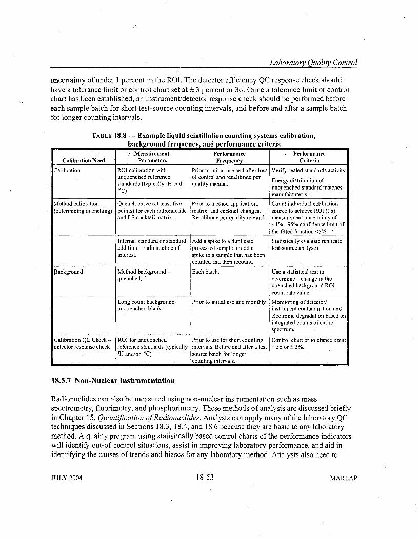
Laboratory Quality Control

uncertainty of under 1 percent in the ROI. The detector efficiency QC response check shouldhave a tolerance limit or control chart set at ± 3 percent or 3a. Once a tolerance limit or controlchart has been established, an instrument/detector response check should be performed beforeeach sample batch for short test-source counting intervals, and before and after a sample batchfor longer counting intervals.

TABLE 18.8 - Example liquid scintillation counting systems calibration,background frequency, and performance criteria

Measurement Performance PerformanceCalibration Need Parameters Frequency Criteria

Calibration ROI calibration with Prior to initial use and after loss Verify sealed standards activity.unquenched reference of control and recalibrate per Energy distribution ofstandards (typically 'H and quality manual.14c) unquenched standard matches

manufacturer's.

Method calibration Quench curve (at least five Prior to method application, Count individual calibration(determining quenching) points) for each radionuclide matrix, and cocktail changes. source to achieve ROI (to)

and LS cocktail matrix. Recalibrate per quality manual. measurement uncertainty of•1%. 95% confidence limit ofthe fitted function <5%

Internal standard or standard Add a spike to a duplicate Statistically evaluate replicateaddition - radionuclide of processed sample or add a test-source analyses.interest, spike to a sample that has been

counted and then recount.

Background Method background - Each batch. Use a statistical test toquenched.* determine a change in the

.quenched background ROIcount rate value.

Long count background- Prior to initial use and monthly. Monitoring of detector/unquenched blank, instrument contamination and

electronic degradation based onintegrated counts of entirespectrum.

Calibration QC Check - ROI for unquenched Prior to use for short counting Control chart or tolerance limit:detector response check reference standards (typically intervals. Before and after a test ± 3a or ± 3%.

'H and/or "4C) source batch for longer_ _ _ counting intervals.

18.5.7 Non-Nuclear Instrumentation

Radionuclides can also be measured using non-nuclear instrumentation such as massspectrometry, fluorimetry, and phosphorimetry. These methods of analysis are discussed brieflyin Chapter 15, Quantification of Radionuclides. Analysts can apply many of the laboratory QCtechniques discussed in Sections 18.3, 18.4, and 18.6 because they are basic to any laboratorymethod. A quality program using statistically based control charts of the performance indicatorswill identify out-of-control situations, assist in improving laboratory performance, and aid inidentifying the causes of trends and biases for any laboratory method. Analysts also need to

JULY 2004 18-53 MARLAP

Laboratory Quality Control

consider detection capabilities, radionuclide equilibrium, half-life, interferences, and blindsamples when using non-nuclear instrumentation.

18.6 Related Concerns

18.6.1 Detection Capability

Issue: The detection capability of an analytical procedure is its ability to distinguish smallamounts of analyte from zero (Chapter 20). The detection capability of a procedure can beestimated nominally and will depend on many factors.

Discussion: In radioanalysis, the most commonly used measure of detection capability is theminimum detectable concentration (Chapter 20). The MDC is defined as the smallest concentra-tion of an analyte that has a specified probability of detection. The MDC is usually estimated as anominal scoping performance measure of an analytical procedure, but a sample-specific versionis reported routinely by many laboratories.

Detection capability is affected by many factors, including counting times, instrument back-ground levels, aliquant volume, yield, decay times, and interferences. The nominal MDC ispresumably based on conservative assumptions about these factors, but measurement conditionsvary. The sample-specific MDC is calculated using the actual measured values of all thesefactors. A high MDC by itself does not indicate that a sample result is invalid or that it cannot beused for its intended purpose. However, if an analysis fails to detect the analyte of interest andthe sample-specific MDC is greater than a detection limit required by contract or otheragreement, it may be necessary to reanalyze the sample in a way that reduces the MDC. Suchdecisions should be made case-by-case, since it is not always cost-effective or even possible toreanalyze a sample, or it may not be feasible to achieve the desired MDC.

Excursions: A high sample-specific MDC can be caused by many factors, including:

" Small sample aliquant;" Low chemical/tracer yield;" Short counting times;* Long decay/short ingrowth time;" High background or blank value; and" Low counting efficiency or sample self-attenuation.

18.6.2 Radioactive Equilibrium

Issue: It is sometimes necessary to ensure that target radionuclides are in radioactive equilibriumwith their progeny, or to establish and correct for disequilibrium conditions. This is particularly

,MARLAP 18-54 JULY 2004

Laboratory Quality Control

applicable for protocols that involve the chemical separation of long-lived radionuclides fromtheir progeny. This is also applicable for nondestructive assays like gamma spectrometry wherephoton emission from progeny is used to determine the concentration of the non-gamma rayemitting parent (see Attachment 14A following Chapter 14 for a more thorough discussion onradioactive equilibrium).

Discussion: Some radionuclides that have long physical half-lives decay to species whose half-lives are shorter by several orders of magnitude. Following chemical separation of the parent, theprogeny can "grow in" within a time frame relevant to analysis and provide measurable radio-active emissions that should be considered in the analytical method. The condition where theparent and progeny radionuclide are equal in activity is called "secular equilibrium." An exampleis 226R, a common, naturally occurring radionuclide in the uranium series with a half-life of about1,600 years. 226Ra is found in water and soil, typically in secular equilibrium with a series ofshorter-lived radionuclides that begins with the 3.8-day-half-life 22 2 Rjn and ends with stable lead.As soon as 226Ra is chemically separated from its progeny in an analytical procedure viacoprecipitation with barium sulfate, its progeny begin to reaccumulate. The progeny exhibit avariety of alpha, beta and gamma emissions, some of which will be detected when the precipitateis counted. The activity due to the ingrowth of radon progeny should be considered when evalua-ting the counting data (Kirby, 1954). If counting is performed soon after chemical separation,secular equilibrium will be substantially incomplete and a sample-specific correction factorshould be calculated and applied. In some cases, it may be necessary to derive correction factorsfor radioactive ingrowth and decay during the time the sample is counting. These factors areradionuclide specific, and should be evaluated for each analytical method.

Secular equilibrium concerns also apply to non destructive assays, particularly for uranium andthorium series radionuclides. Important radionuclides in these series (e.g., 23"U and 23.Th) havephoton emissions that are weak or otherwise difficult to measure, while their shorter-livedprimary, secondary or tertiary progeny are easily measured. This allows for the parents to bequantified indirectly, i.e., their concentration is determined by measuring their progeny andaccounting for the amount of parent-progeny equilibrium. The amount of parent-progeny secularequilibrium is fundamental to these analyses, and data should be scrutinized to insure that theamount is valid.

When several radionuclides from one decay chain are measured in a sample, observed activityratios can be compared to those predicted by decay and ingrowth calculations, the history of thesample and other information. For example, undisturbed soil typically contains natural uraniumwith approximately equal activities of 238U and 234U, while water samples often have verydifferent 238U/ 234U ratio. Data from ores or materials involved in processing that could disruptnaturally occurring relationships require close attention in this regard.

All numerical protocols (electronic and manual) should be evaluated to determine if there is bias

JULY 2004 18-55 MARLAP

Laboratory Quality Control

with respect to correction factors related to equilibrium concerns. This includes a check of allconstants and units used to derive such correction factors, as well as the use of input data thatunambiguously state the time of all pertinent events (chemical separation and sample counting).The analyst should ensure that samples requiring progeny ingrowth are held for sufficient timebefore counting to establish secular equilibrium. Limits for minimum ingrowth and maximumdecay times should be established for all analytical methods where they are pertinent. Foringrowth, the limits should reflect the minimum time required to ensure that the radionuclide(s)of interest has accumulated sufficiently to not adversely affect the detection limit or uncertainty.Conversely, the time for radioactive decay of the radionuclides of interest should be limited suchthat the decay factordoes not elevate the MDC or adversely affect the measurement uncertainty.These will vary depending on the radionuclide(s) and'analytical method.

Excursions: Samples where equilibrium is incorrectly assumed or calculated will produce datathat do not represent the true sample concentrations. It is difficult to detect errors in equilibriumassumptions or calculations. Frequently, it takes anomalous or unanticipated results to identifythese errors. In these cases, analysts need to know the sample history or characteristics beforeequilibrium errors can be identified and corrected. Some samples may not be amenable tonondestructive assays because their equilibrium status cannot be determined; in such cases, otheranalytical methods are indicated.

Examples:

Isotopic Distribution - Natural, Enriched and Depleted Uranium: Isotopic distribution isparticularly important with respect to uranium, an element that is ubiquitous in nature in soilsand also a contaminant in many site cleanups. The three predominant uranium isotopes ofinterest are 238U, 234U, and 235U, which constitute 99.2745, 0.0055, and 0.72 atom percent,respectively, of "natural" uranium, 3 i.e., uranium as found in nature (Parrington et al., 1996).However, human activities related to uranium typically involve changing the ratio of naturaluranium by separating the more readily fissionable 235U from natural uranium to producematerial "enriched" in 235U, for use in fuel cycle and nuclear weapons related activities.4

Typical 235U enrichments range from 2 percent for commercial reactor fuels to greater than 90percent 235U for weapons. The enrichment process also produces material that is "depleted" in235U, i.e., the uranium from which the 235U was taken. While the 235U concentrations ofdepleted uranium are reduced relative to natural ores, they still can be measured by several.assay techniques. This gives rise to uranium with three distinct distributions of 238U, 235U, and"34U, referred to as "natural," "enriched," and "depleted" uranium. Because 235U, 231U, and

3 The "natural abundance" of 2351U of 0.72 atom percent is a commonly accepted average. Actual values from

specific ore samples vary.

4 Enriched and depleted refer primarily to 235U.

MARLAP 18-56 JULY 2004

LaboratoTy Quality Control

U are alpha emitters with considerably different physical half-lives and specific activities, ameasurement of a sample's total uranium alpha activity cannot be used to quantify thesample's isotopic composition or uranium mass without knowing if the uranium is natural orhas been enriched or depleted in 235U. However' if this information is known, measurementand distribution of the sample's uranium alpha activity can be used to infer values for asample's uranium mass and for the activities of the isotopes . 38U, 23"U, and 234U. This ratiocan be determined directly or empirically using mass or alpha spectrometry, techniques whichare time and cost intensive, but which provide the material's definitive isotopic distribution.It is often practical to perform mass or alpha spectrometry on representative samples from asite to establish the material's isotopic distribution, assuming all samples from a given areaare comparable in this respect. Once established, this ratio can be applied to measurements ofuranium alpha activity to derive activity concentrations for 238U, 234U, and 235U data.

18.6.3 Half-Life

Issue: Radionuclides with short half-lives relative to the time frame of the analysis may decaysignificantly from the time of sample collection or chemical separation to counting. In somecases, this decay will cause the ingrowth of other short-lived radionuclides. In both instances,sample-specific factors should be applied to correct the sample's observed counting/disintegra-tion rate. Also, determination of half-life could indicate sample purity. If radioactive impuritiesare not appropriately corrected, analytical errors will occur. Repetitive counting of the test sourcemay confirm the radionuclide's half-life, and thus the radioactive purity of the test source.

Discussion: When assaying for short-lived radionuclides, data should be corrected for decay overthe time period between sample collection and counting. For example, operating power reactorsroutinely assay environmental samples for "3l, a fission product with about an eight-day half-life.Samples may be counted for several days up to two weeks, during which time their "3I concen-tration is decreasing via radioactive decay. Using the eight-day half-life, the counting data shouldbe decay-corrected to the ending time of collection in the field and corrected for decay before andduring counting. If desired, environmental samples can be decay-corrected to a time other thansample collection.

Half-life considerations also apply to radionuclide ingrowth. Certain radionuclides are assayed byan initial chemical separation, which begins a time period over which their direct progeny areallowed to reach a near-secular equilibrium condition. This is followed by additional chemicalseparation, purification, and counting of the progeny. The degree of the progeny's ingrowth iscalculated based on the radionuclides' half-lives and the elapsed time between the two chemicalseparations. Allowance should also be made for the progeny's decay from separation to countingand for decay that occurred while counting, if applicable. Two examples are the beta emittingradionuclides 228Ra and 9"Sr: they are quantified by measuring the direct progeny of each, 228Acand 90Y, respectively. For airborne concentrations of 2 1 Rn, sample collection and analytical

JULY 2004 18-57 MARLAP

Laboratory Quality Control

methods should incorporate concerns related to the short-lived progeny of other radon species,such as 22.Rn. Other half-life related considerations apply to alpha spectrometry when assayingsamples for uranium and thorium chain radionuclides. Samples that have been allowed to sit forseveral weeks may accumulate short-lived radionuclides that have alpha emissions whoseenergies are in close proximity to target radionuclides. These can interfere with quantitativeanalyses of the target radionuclides. Chemical yield tracers used in alpha spectrometry, such as234Th and . 32U, can cause this effect due to their short-lived progeny and all chemical yield tracersshould be scrutinized for this potential prior to their use in analytical methods. Radionuclidespecific limits for minimum ingrowth and maximum decay times should be established for allanalytical methods where they are pertinent. These should be based on limiting the adverse effectof such calculations on the detection limit and measurement uncertainty. All analytical methodsinvolving computational corrections for radioactive decay of the target species should beevaluated relative to half-life and secular equilibrium related concerns. This evaluation should beincorporated in the routine data review process that is performed on all analytical results.

A good source for radionuclide half-lives and other nuclear data can be found at the BrookhavenNational Laboratory's National Nuclear Data Center (www.nndc.bnl.gov/nndc/nudat/). Usingthis data source will ensure consistency within and among laboratories, and will provide analystswith the current values.

Excursions: Samples that are assayed by "non destructive" techniques like gamma spectrometrymay provide indications of potential complications due to half-life related considerations.Because the assay provides information on photon emitting radionuclides in the sample, theanalyst can develop appropriate corrections for half-life related phenomena. However, non-spectrometric techniques like gas flow proportional counting are essentially gross countingprocedures that record all events without any indication of their origin. Therefore, these datashould be evaluated to ensure they are free from half-life related considerations (e.g.,radionuclide purity).

Samples with short-lived radionuclide concentrations at or near environmental background willexperience elevated detection limits and increased measurement uncertainty if there is excessiveelapsed time between sample collection and counting. Because of the magnitude of the additionalcorrection (decay) factor for these samples, they usually have a larger measurement uncertaintycompared to longer-lived radionuclides, given equal measurement and sample conditions andparameters.

18.6.4 Interferences

Issue: Chemical or radionuclide interferences can produce erroneous results or increasedmeasurement uncertainty.

MARLAP 18-58 JULY 2004

Laboratoiy Quality Control

Discussion: Analytical samples, particularly environmental samples, are often chemicallycomplex. This complexity may include chemical constituents that interfere with an analyticalmethod to the point that they require modification of the method. Examples of modificationsinclude limiting the size of the sample aliquant, quantifying interfering compounds through otheranalyses (radiometric and non-radiometric) and changing time periods to allow adequateingrowth of target radionuclides or decay of interferences.

A common example is groundwater or well water that contains high concentrations of salts ordissolved solids, so that screening for gross alpha activity produces erratic or anomalous results.For such samples, it may be necessary to limit the aliquant volume with the resulting increase indetection limit and measurement uncertainty. There is a salt concentration at which thisprocedure cannot overcome the interferences and should not be used.

Samples that contain natural concentrations of stable or radioactive compounds that are addedduring an analytical procedure (e.g., carrier or tracer) may also cause interference problems.Because barium is used as a carrier, water samples that contain a high concentration of bariummay provide inaccurate carrier yields when screened for alpha-emitting radium isotopes.Quantifying the sample's barium content prospectively via a non-radiometric technique (e.g.,atomic absorption) would be required to correct for this interference. With respect to radioactivecompounds, two examples are provided. The first involves the radiochemical procedure fordetermining 228Ra in drinking water that separates radium via coprecipitation with barium sulfate.The precipitate is allowed to come to equilibrium with its direct progeny 228Ac, which is separa-ted via co-precipitation with yttrium oxalate, purified, mounted and counted. The yttriumprecipitate also carries 90Y, the direct progeny of 9 Sr, a fission product often found in environ-mental samples as a result of atmospheric weapons testing and nuclear fuel cycle activities. Theresults of samples assayed for 228Ra that contain measurable amounts of 9̀Sr require correctionsbecause of the differences in half-lives (228Ac with a 6-hour half-life versus 90Y with a half-life ofabout 64 hours) or other parameters. The second example involves alpha spectrometry proce-dures that use tracers to determine chemical yield. For example, 234Th is used as a chemical yieldtracer for isotopic thorium analyses. The approach assumes that the sample's inherent concentra-tion of the tracer radionuclide is insignificant such that it will not interfere with the tracer'sability to accurately represent the sample's chemical yield. Samples that contain measurableamounts of these radionuclides may produce excessive interference and may not be amenable tothis procedure.

Alpha spectra should be checked for radionuclide interferences (e.g., a 232Th peak in uraniumspectra). If the 232Th peak is present due to incomplete chemical separation, 23°Th may representinterference in the 2 34U determination. Data should be corrected or the samples reanalyzed withbetter target-radionuclide purification.

Each analytical method should be evaluated with respect to interferences during the method-

JULY 2004 18-59 MARLAP

Laboratory Quality Control

validation stage. Such evaluations can be based on available information and, if properlydocumented, can serve as the basis for developing the range of applicability, which becomes anintegral part of the protocol. Evaluating performance indicators aids in the identification ofsamples that have interferences. All performance criteria would be protocol specific, and haveclearly established acceptance ranges that incorporate the potential interferences discussed above.

Excursions: Interfering elements can affect measurement results in several ways. For example,large amounts of non-analyte elements may overload ion exchange resins, affecting the resin'sability to collect all of the analyte. In addition, spiking elements, already in the sample prior topreparation, may cause matrix spike results to exceed acceptance limits.

Carrier/tracer yields exhibiting gradual changes that appear to be correlated with a batch or groupof samples from the same sampling location may indicate potentially interfering conditions. Asignificant decrease in the carrier/tracer yield may indicate that the analytical method is notfunctioning as planned. Yields that are significantly low or in excess of 100 percent may becaused by competing reactions within the sample matrix, or by the presence of an inherent carrieror tracer within the sample.

For screening analyses, e.g., gross alpha or beta, large changes in counting efficiencies or erraticcounting data can reflect the presence of salts. Samples of this type are hygroscopic and continueto gain weight following preparation as they absorb moisture from the air. These changes couldbe detected by reweighing the planchets directly prior to counting. These samples can be conver-ted to oxides by carefully holding them over the open flame of a laboratory burner; however, thiswill cause losses of volatile radionuclides, such as "10Po and '37Cs, which have alpha and betaemissions, respectively. An alternative approach is to thoroughly dry each planchet, record theweight and count it immediately, followed by a post-counting weighing to ensure that the weightdid not change significantly over the measurement period. This approach may not be practical forall laboratories.

18.6.5 Negative Results

Issue: When an instrument background measurement is subtracted from a measurement of a low-'activity sample, it is possible to obtain a net activity value less than zero.

Discussion: Many factors influence the evaluation of negative results. The simplest case occurswhen the background measurement is unbiased and both the gross counts and background countsare high enough that the distribution of the net count rate is approximately normal. In this case,normal statistics can be used to determine whether a negative result indicates a problem. Forexample, if a sample contains zero activity, there is a very small probability of obtaining a netcount rate more than two-and-a-half or three standard deviations below zero (i.e., negativevalue). Since the combined standard uncertainty is an estimate of the standard deviation, a result

MARLAP 18-60 JULY 2004

Laboratory Quality Control

that is less than zero by ,more than three times its combined standard uncertainty should beinvestigated. In fact, if a blank sample is analyzed using an unbiased measurement process,negative results can be expected about 50 percent of the time. As long as the magnitudes ofnegative values are comparable to the estimated measurement uncertainties and there is nodiscernible negative bias in a set of measurements, negative results should be accepted aslegitimate data and their uncertainty should be assessed. On the other hand, if a sample activityvalue is far below zero, there may be a reason to investigate the result. A large percentage ofnegative results may also indicate a problem, even if all of the results are near zero. Wheninstrument backgrounds are extremely low, statistics based on a normal distribution may not beappropriate (Chapter 19).

A preponderance of results that are negative, even if they are close to zero, indicates either asystematic error or correlations between the results. If the results are measured independently, apattern of negative results indicates a bias, which requires investigation.

Excursions: Negative results occur routinely when samples with low levels of activity areanalyzed, but a result should seldom be more than a few standard deviations below zero. Possiblecauses for extremely negative results or for an excessive number of negative values include:

" Instrument failure (low sample counts or high blank counts);• Positive bias in the background or reagent blank measurement;• Overestimation of interferences;" Wrong or inappropriate background data;- Data transcription error; or" Calculation error.

18.6.6 Blind Samples

Issue: The performance of the analytical method should be assessed independently on a regularbasis. This assessment is achieved through the use of blind samples that provide an objectivemeans of evaluating the laboratory's performance when analyzing specific analytes and matrices.Blind samples can be internal or external, and either single or double. External blind perfor-mance-testing (PT) samples (also called performance-evaluation, or PE, samples) are used forQA purposes and also can provide information that is useful to laboratory QC.

Discussion: A blind sample is a sample whose concentration is not known to the analyst, andwhose purpose is to assess analytical performance. Regardless of their nature, blind samples areeffective only when their contents are unknown to the analysts. The preparation of all blind andother performance assessment samples is usually designated as a QA function. The QA stafffunctions independently from personnel responsible for sample processing and analysis. Blindsamples consist of a matrix routinely processed by the laboratory that contains a known amount

JULY 2004 18-61 MARLAP

Laboratoty Quality Control

of one or more analytes (radionuclides). A blind sample also may take the form of a replicatesample that is submitted for analysis such that its composition and origin are unknown to theanalyst. These can be split samples (if run in the same batch) or spiked samples, and are preparedand submitted by an independent group either within the organization (internal), or from anindependent organization (external). Performance on blind samples should be an integral part ofthe laboratory's quality system, which includes routine evaluation of their analytical resultsagainst specific performance criteria. For example, analysis of blind samples should be evaluatedfor relevant performance indicators. Data that fall outside an acceptance criterion may indicateloss of control in sample chemical processing, radiometric determination (counting) or otheraspects of the analytical process. The ability to prepare blind samples depends fundamentally onthe ability to obtain the appropriate combination of matrix with a radionuclide of a well-knownconcentration, ideally traceable to NIST or other appropriate certifying body. Also important arethe expertise and experience of the preparer of the blind samples, proven and verifiedmethodologies used for the blind samples, and detailed documentation. The use of blind samplesassumes that their physical, chemical and radiological nature are similar to routine samples andcompatible with the analytical methods employed at the laboratory.

When the analyst is aware that the sample is a blind sample but does not know the concentration,these samples are called single blinds. The analyst may know what analytes the blind samplecontains, but not the analyte's concentration. Single blinds and other internal samples of this typeare generally prepared by an organization's QA personnel that are independent of the samples'analyses. External single blind samples are available and can be obtained from several sources.

A double blind sample is a PT sample whose concentration and identity as a PT sample is knownto the submitter but not to the analyst. The double blind sample should be treated as a routinesample by the analyst, so it is important that the double blind sample be identical in appearanceto routine samples. A replicate routine sample would be considered a double blind PT sample.However, samples having sufficient measurable analyte are the most desirable as double blindsamples for measuring precision. In general, a double blind is thought to be a more rigorousindication of the laboratory's performance, since analysts and other laboratory personnel maytake special precautions when analyzing known PT samples, in anticipation of the greaterscrutiny associated with such samples. This should not happen with double blind samples, sincethere should be no way to distinguish them from routine samples. However, true double blindsamples are difficult to prepare.

INTERNAL BLIND SAMPLES. Internal blind samples are prepared by the laboratory's QApersonnel. Internal blind samples assess several aspects of the analytical process. They allowthe laboratory to demonstrate that it can successfully process routine samples for a specificanalysis; in other words, they get a measured result within accepted limits. They provide anauditable, empirical record against specific quality performance criteria. They also demons-trate the efficacy of analytical methods and areas in need of adjustment. Double blindsamples can pose logistical problems. It may be difficult to prepare internal double blind

MARLAP 18-62 JULY 2004

Laboratory Quality Control

samples and submit them to the laboratory for analysis successfully disguised as routinesamples. Certain replicate routine samples are the. exception. Evaluation criteria should beestablished to identify when conditions are out of acceptance limits.

EXTERNAL BLIND SAMPLES. External blind samples are those prepared by an organizationoutside that laboratory. This may be helpful with respect to ensuring that the analyte concen-trations are truly unknown to the analyst; external blinds may offer a greater variety ofmatrices and analytes than can easily be produced within the laboratory and augment thelaboratory's internal quality control program. Alternatively, if external blinds are notappropriate to the laboratory's programs, they will be of limited utility.

If statistical differences between observed and known values typically arise, these should beinvestigated thoroughly, as they indicate areas where important details of the analyticalprocess may have been overlooked. Often a laboratory's observed values agree with theknown value within acceptable tolerances, but are biased high or low. Careful documentationof the laboratory's performance in this regard can assist in characterizing the fluctuations of ameasurement system or analytical method. Like other performance indicators, large or suddenchanges in bias require scrutiny.

Blind samples should be an integral part of the laboratory's quality control program and theyshould be processed according to a predetermined schedule. Important sources of external blindsamples include the NIST Radiochemistry Intercomparison Program (NRIP), National VoluntaryAccreditation Program (NVLAP/EPA), Food and Drug Administration, DOE Lab AccreditationProgram (DOELAP), Quality Assessment Program (DOE QAP), Multi-Analyte PerformanceEvaluation Program (DOE MAPEP), and several commercial vendors.

Excursions: The excursions typically encountered with analytical methods for specificparameters (carrier/tracer recovery, lack of precision, elevated backgrounds, etc.) apply to blindsamples as well. Additionally, instances where the analysis of external blinds produces valuesthat do not agree with the known values, may indicate that instrument calibrations or othercorrection factors require reevaluation. Problems revealed by the analysis of blind blank samplescan indicate a problem (e.g., bias, blunder) within the laboratory, or conditions where the currentprotocol is inadequate. Excursions discovered while analyzing samples from external PTprograms should be addressed.

18.6.7 Calibration of Apparatus Used for Mass and Volume Measurements

Issue: Fundamental to all quantitative analysis is the use of the proper masses and volumes.Analysts should perform careful gravimetric and volumetric measurements (especially in thepreparation of calibration solutions, test sources, and reagents) in Order to achieve the desiredlevels of precision and bias in each analytical method. Therefore. laboratory balances and

JULY 2004 18-63 MARLAP

Laboratoiy Quality Control

volumetric glassware and equipment should be calibrated and checked periodically to maintainthe desired method performance levels. This section discusses the calibrations of laboratorybalances and volumetric glassware and equipment. See Chapter 19, Attachment F, for furtherdiscussion on mass measurements.

Discussion: Laboratory balances should be periodically calibrated and checked. Most balancesare typically calibrated and certified by the manufacturer once a year. These calibrations areperformed to achieve the manufacturer's specified tolerances for each balance. A calibrationcertificate is supplied to the laboratory. In addition to this yearly calibration, daily calibrationchecks should be performed by the laboratory. Some laboratories check the balances once a dayor at the time of each use. Any balance failing the daily calibration check should be taken out ofservice. Ordinarily, ASTM E617 Class 1 or 2 masses are used to perform the daily calibrationcheck, dependinggn application. Over time; daily wear and tear on the masses can affectcalibration, so it is a good idea to get them periodically re-certified or to purchase new masses.

Volumetric glassware and equipment, especially those used in the preparation of instrumentcalibration solutions and laboratory control samples, should be calibrated to the desired level ofaccuracy. Calibration can either be performed by the manufacturer of the equipment or bylaboratory personnel. Calibration certificates for volumetric pipets and flasks are provided by themanufacturer at the time of purchase. Borosilicate and Pyrex ® volumetric glassware will hold itscalibration indefinitely provided that it is not exposed to hydrofluoric acid, hot phosphoric acidor strong alkalis, and that it is not heated above 150 'C when drying. Any glass volumetric pipetwith a damaged tip should be discarded or re-calibrated. The manufacturer of volumetricautomatic pipetting equipment calibrates the equipment and provides a certificate at the time ofpurchase. The re-calibration of automatic equipment should be performed annually and can beperformed by the manufacturer, calibration specialty companies, or in-house laboratorypersonnel. Outside calibration services should provide a calibration certificate.

Laboratory personnel can calibrate and check volumetric apparatus using procedures like thosespecified in ASTM E542. Typically calibrations use volumes of water and are gravimetricallybased. Volumes are corrected for temperature and atmospheric pressure and require thoroughlycleaned glassware, standard procedures for setting and reading the water meniscus, and accuratebalances and thermometers.

Volumetric glassware is calibrated either "to contain" (TC) or "to deliver" (TD). Glasswaredesignated as "to contain" has a mark referred to as the "fiducial mark." When the vessel is filledto that mark, it "contains" the designated volume. Emptying the vessel does not have anyquantitative measure associated with it. "To deliver" glassware is not to be completely emptiedor "blown out." Specified volumes for TD glassware do not include the residual left from surfaceadhesion and capillary action. TD glassware will perform with accuracy only when the innersurface is so scrupulously clean that the water wets it immediately and forms a uniform filmwhen emptying,

MARLAP 18-64 JULY 2004

Laboratoty Quality Control

18.7 References

18.7.1 Cited Sources

American National Standards Institute/International Standards Organization/American Societyfor Quality Control (ANSIISO/ASQC) A3534-2. "Statistics-Vocabulary and Symbols-Statistical Quality Control." 1993.

American National Standards Institute/American Society for Quality Control (ANSI/ASQC) E4."Specifications and Guidelines for Quality Systems for Environmental Data Collection andEnvironmental Technology Programs." 1994.

American National Standards Institute (ANSI) Ni. 1. "American Nuclear Standard Glossary ofTerms in Nuclear Science and Technology." 1976.

American National Standards Institute (ANSI) N 15.37. "Guide to the Automation ofNondestructive Assay Systems for Nuclear Material Control." 1981.

American National Standards Institute (ANSI) N42.12. "Calibration and Usage of Thallium-Activated Sodium Iodide Detector Systems for Assay of Radionuclides." 1994.

American National Standard Institute (ANSI) N42.23. "Measurement and AssociatedInstrumentation Quality Assurance for Radioassay Laboratories." 2003.

American Society for Testing and Materials (ASTM) D3648. Standard Practices for theMeasurement of Radioactivity, 1995, West Conshohocken, Pennsylvania.

American Society for Testing and Materials (ASTM) D6299. Standard Practice for ApplyingStatistical Quality Assurance Techniques to Evaluate Analytical Measurement SystemPerformance, 2000, West Conshohocken, Pennsylvania.

American Society for Testing and Materials (ASTM) E542. Standard Practice for Calibration ofLaboratory Volumetric Apparatus, 2000, West Conshohocken, Pennsylvania.

American Society for Testing and Materials (ASTM) E617. Standard Specification forLaboratory Weights And Precision Mass Standards, 1997, West Conshohocken,Pennsylvania.

American Society for Testing and Materials (ASTM) E 181. Standard Test Methods for DetectorCalibration and Analysis of Radionuclides, 1998, West Conshohocken, Pennsylvania.

JULY 2004 18-65 MARLAP

Laboratory Quality Control

American Society for Testing and Materials (ASTM) E882. Standard Guide for Accountabilityand Quality Control in the Chemical Analysis Laboratory, 1998, West Conshohocken,Pennsylvania.

American Society for Testing and Materials (ASTM) MNL 7. Manual on Presentation of Dataand Control Chart Analysis ASTM Manual Series, "h Edition, 2002

Friedlander, G., Kennedy, JW., Macias, E.S., and Miller, J.N. 1981. Nuclear andRadiochemistry. 3rd Edition, John Wiley and Sons, New York.

Gilmore, G. and Hemingway, J.D. 1995. Practical Gamma-Ray Spectrometry. Wiley, Chichester,England.

International Standards Organization (ISO) 5725-1. Accuracy (Trueness and Precision) ofMeasurement Methods and Results-Part 1: General Principles and Definitions. 1994,Geneva, Switzerland.

International Standards Organization (ISO) 7870. Control Charts - General Guide andIntroduction. 1993, Geneva, Switzerland.

International Standards Organization (ISO) 7873. Control Charts for Arithmetic Average WithWarning Limits. 1993, Geneva, Switzerland.

International Standards Organization (ISO) 7966. Acceptance Control Charts. 1993, Geneva,Switzerland.

International Standards Organization (ISO) 8258. Shewhart Control Charts. Corrected, 1993,Geneva, Switzerland.

International Standards Organization/International Electrotechnical Commission (ISO/IEC)17025. General Requirements for the Competence of Testing and Calibration Laboratories.December 1999, 26 pp.

Kirby, H.W. 1954. "Decay and Growth Tables for the Naturally Occurring Radioactive Series."Anal. Chem. 26:6, p. 1063-1071.

Lin, Z., Inn, K.G.W., and Fiilben, J. J. 2001. An alternative statistical approach forinterlaboratory comparison data evaluation. J. Radioanalytical and Nuclear Chemistry,248:1, 163-173.

National Council on Radiation Protection and Measurements (NCRP) 58: A Handbook ofRadioactivity Measurement Procedures, Second Edition. Bethesda, MD. February 1985.

MARLAP 18-66 JULY 2004

Laboratory Quality Control

National Environmental Laboratory Accreditation Conference (NELAC). 2002. NELACStandards. Appendix D, Essential Quality Control Requirements. Available at: www.epa.gov/ttn/nelac/2002standards.html.

Parrington, J.R., Knox, H.D., Breneman, S.L., Feiner, F., and Baum, E.M. 1996. Nuclides andIsotopes.- Chart of the Nuclides. 15th Edition. Lockheed Martin and.General Electric.

18.7.2 Other Sources

American National Standards Institute (ANSI).N42.22. "Traceability of Radioactive Sources tothe National Institute of Standards and Technology (NIST) and Associated InstrumentQuality Control." 1995.

Chase, G.D. and Rabinowitz, J.L. 1969. Principles of Radioisotope Methodology. 3rd Edition,Burgess Publishing Co., Minneapolis, MN/N.

U.S. Environmental Protection Agency (EPA). 1977. Handbook for Analytical Quality Controlin Radioanalytical Laboratories. EPA-600-7-77-088.

U.S. Environmental Protection Agency (EPA). 1980a. Prescribed Procedures for Measurementof Radioactivity in Drinking Water-Procedure 904. 0, Determination of Radium-228 inDrinking Water. EPA 600-4-80-032.

U.S. Environmental Protection Agency (EPA). 1980b. Prescribed Procedures for Measurementof Radioactivity in Drinking Water-Procedure 908. 1 for Total Uranium in Drinking Water.EPA 600-4-80-032.

U.S. Environmental Protection Agency (EPA). 2001. Guidance for the Preparation of StandardOperating Procedures (SOPs) for Quality-rela.ted Documents. QA/G-6. EPA/240/B-0 1/004.Available at www.epa.gov/quality/qa-docs.html.

Kanipe, L.G. 1977. Handbook for Analytical Quality Control in Radioanalytical Laboratories.U.S. Environmental Protection Agency, Washington, DC. EPA/600/7-77-088.

Taylor, B.N. and C.E. Kuyatt (2003). Guidelines for Evaluating and Expressing the Uncertaintyof NIST Measurement Results. National Institute of Standards and Technology (NIST),Gaithersburg, MD 20899-0001. Technical Note 1297. Available at: http://physics.nist.gov/cuu/Uncertainty/bibliography.html.

Zeigler, L.H. and Hunt, H.M. 1977. Quality Control for Environmental Measurements UsingGamma-Ray Spectrometry. EPA/600-7-77-144.

JULY 2004 18-67 MARLAP

ATTACHMENT 18AControl Charts

18A.1 Introduction

This attachment provides statistical details to augment Section 18.3.2. The term "statisticalquality contiol" refers to QC based on statistical principles. Generally, statistical QC in thelaboratory applies the principles of hypothesis testing, with varying degrees of rigor, to makeinferences about a measurement system or process. The primary tool for statistical QC is thecontrol chart.

An important reason to establish statistical QC in the laboratory is to ensure that measurementuncertainties are properly estimated. The uncertainty estimate that accompanies a measured valuemay be misleading unless the measurement process is in a state of statistical control. Statisticalcontrol implies that the distribution of measured results is stable and predictable. It exists whenall the observed variability in the process is the result of random causes that are inherent in theprocess. The existence of variability due to "assignable" causes, including instrumental andprocedural failures and human blunders, which are not inherent in the process, implies that theprocess is unpredictable and hence "out of control."

Statistical QC procedures are designed to detect variations due to assignable causes. When suchvariability is detected, specific corrective action is required to determine the cause and bring themeasurement process back into a state of statistical control. Laboratory QC procedures should bedefinitive enough to detect variations in the measurement system that could have a significantimpact on measurement uncertainties.

Statistical QC also may be used in the laboratory to monitor method performance parameters,such as chemical yield, to ensure that the measurement system is performing as expected. How-ever, the need for. corrective action in the case of a low yield may not be as urgent as in the caseof a malfunctioning radiation counter, since the latter is much more likely to cause underestima-tion of measurement uncertainties.

The following sections describe the various types of control charts introduced in Section 18.3.2,including the X chart, X chart, R chart, and variants of the c chart and u chart for Poisson data.

18A.2 XCharts

Procedure 18.1, shown below, may be used to determine the central line, control limits, andwarning limits for an X chart. Ideally, the data distribution should be approximately normal,although the X chart is often used with other types of distributions.

JULY 2004 18-69 MARLAP

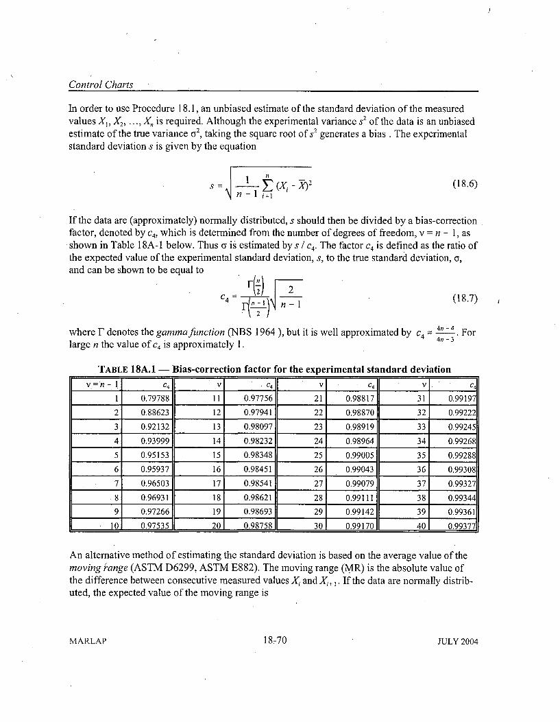
Control Charts

In order to use Procedure 18.1, an unbiased estimate of the standard deviation of the measuredvalues X,, X 2, ... , X, is required. Although the experimental variance s2 of the data is an unbiasedestimate of the true variance a2, taking the square root of s2 generates a bias . The experimentalstandard deviation s is given by the equation

I n

S _ E •(-X)2 (18.6)n - I (=1

If the data are (approximately) normally distributed, s should then be divided by a bias-correctionfactor, denoted by c4, which is determined from the number of degrees of freedom, v = n - 1, asshown in Table 1 8A- 1 below. Thus cy is estimated by s / c4. The factor c4 is defined as the ratio ofthe expected value of the experimental standard deviation, s, to the true standard deviation, a,and can be shown to be equal to

c 4 n - (18.7)C4~()n-l

where F denotes the gamma function (NBS 1964 ), but it is well approximated by c4 4n - 3. Forlarge n the value of c4 is approximately 1.

TABLE 18A.1 - Bias-correction factor for the experimental standard deviation

v n1 C4 V C4 V C4 V C4

1 0.79788 11 0.97756 21 0.98817 31 0.99197

2 0.88623 12 0.97941 22 0.98870 32 0.99222

3 0.92132 13 0.98097 23 0.98919 33 0.99245

4 0.93999 14 0.98232 24 0.98964 34 0.99268

5 0.95153 15 0.98348 25 0.99005 35 0.99288

6 0.95937 16 0.98451 26 0.99043 36 0.99308

7 0.96503 17 0.98541 27 0.99079 37 0.99327

8 0.96931 18 0.98621 28 0.99111 38 0.99344

9 0.97266 19 0.98693 29 0.99142 39 0.99361

10 0.97535 20 0.98758 30 0.99170 40 0.99377

An alternative method of estimating the standard deviation is based on the average value of themoving range (ASTM D6299, ASTM E882). The moving range (MR) is the absolute value ofthe difference between consecutive measured values X• and X•, •. If the data are normally distrib-uted, the expected value of the moving range is

MARLAP 18-70 JULY 2004

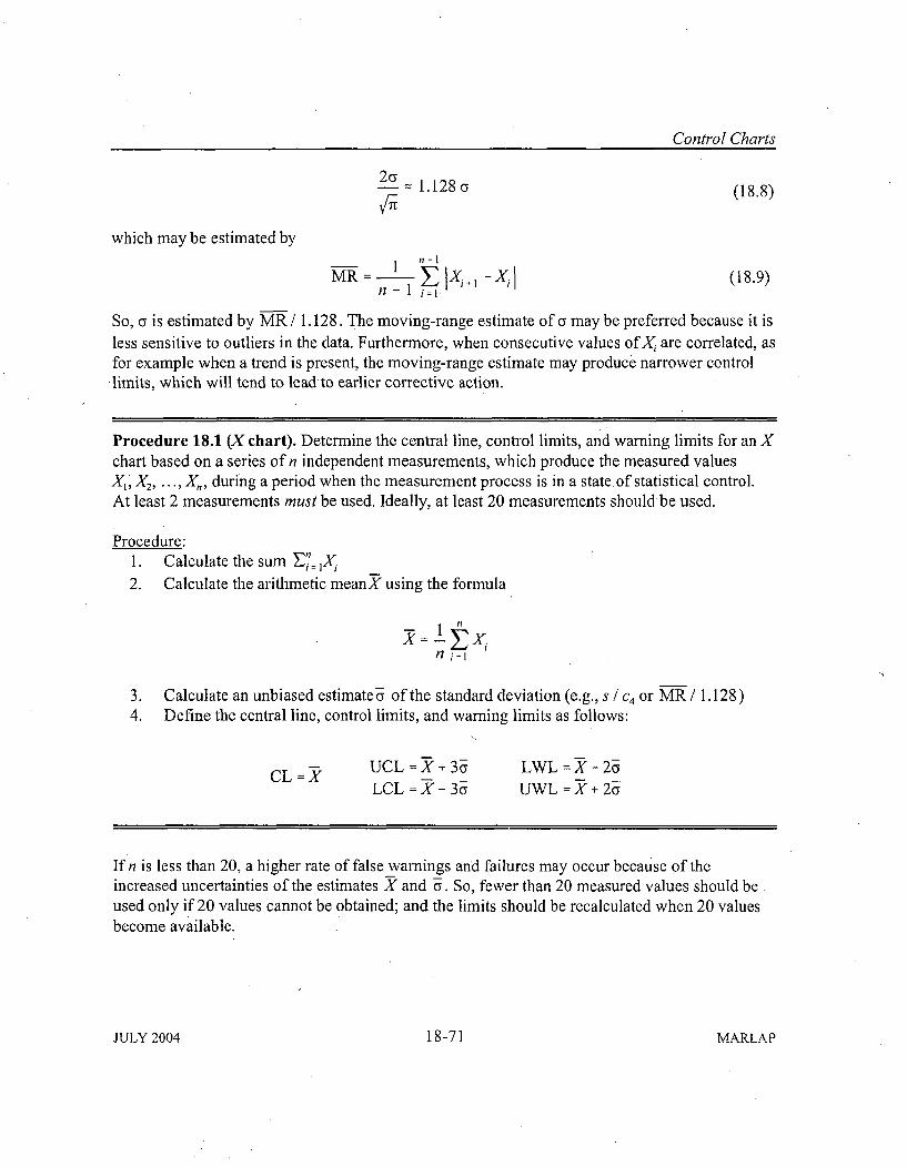
Control Charts

2 (y 1.128 a (18.8)

which may be estimated by

MR 1 (18.9)n 1i=1

So, o is estimated by MR / 1.128. The moving-range estimate of a may be preferred because it isless sensitive to outliers in the data. Furthermore, when consecutive values of Xi are correlated, asfor example when a trend is present, the moving-range estimate may produce narrower controllimits, which will tend to lead to earlier corrective action.

Procedure 18.1 (X chart). Determine the central line, control limits, and warning limits for an Xchart based on a series of n independent measurements, which produce the measured valuesX1' X2, ... , X5, during a period when the measurement process is in a state of statistical control.At least 2 measurements must be used. Ideally, at least 20 measurements should be used.

Procedure:1. Calculate the sum Y71 Xi2. Calculate the arithmetic meanX using the formula

n

n' j=1

3. Calculate an unbiased estimates of the standard deviation (e.g., s / c4 or MR/ 1.128)4. Define the central line, control limits, and warning limits as follows:

CL UCL=_ + 3 LWL = X - 2aLCL=X-3 3o UWL=X+2a2

If n is less than 20, a higher rate of false warnings and failures may occur because of theincreased uncertainties of the estimates X and -. So, fewer than 20 measured values should beused only if 20 values cannot be obtained; and the limits should be recalculated when 20 valuesbecome available.

JULY 2004 18-71 MARLAP

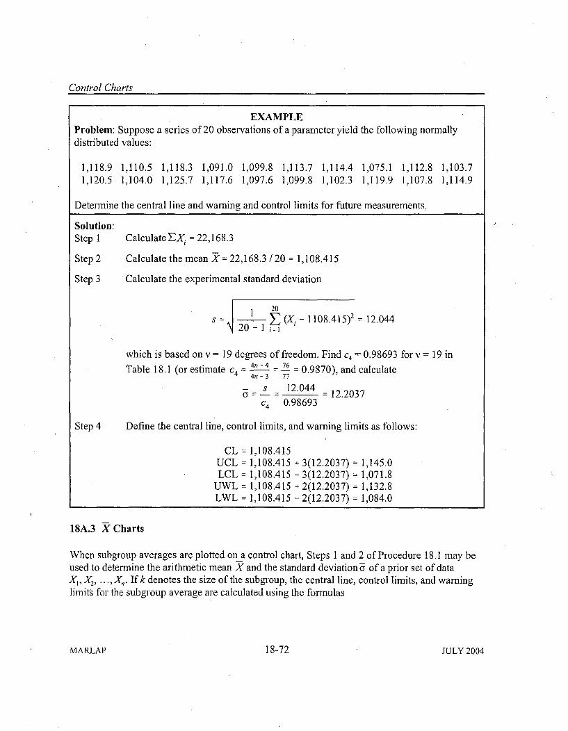
Control Charts

EXAMPLEProblem: Suppose a series of 20 observations of a parameter yield the following normallydistributed values:

1,118.9 1,110.5 1,118.3 1,091.0 1,099.8 1,113.7 1,114.4 1,075.1 1,112.8 1,103.71,120.5 1,104.0 1,125.7 1,117.6 1,097.6 1,099.8 1,102.3 1,119.9 1,107.8 1,114.9

Determine the central line and warning and control limits for future measurements.

Solution:Step 1 Calculate EX. = 22,168.3

Step 2 Calculate the mean X = 22,168.3 /20 = 1,108.415

Step 3 Calculate the experimental standard deviation

1 20s = E (Xi - 1108.415) =12.04420 - I M

which is based on v = 19 degrees of freedom. Find c4 = 0.98693 for v = 19 in

Table 18.1 (or estimate c4 n - =4 76 = 0.9870), and calculate4n - 3 77

- s _ 12.044G =-- . =12.2037

c4 0.98693

Step 4 Define the central line, control limits, and warning limits as follows:

CL = 1,108.415UCL = 1,108.415 + 3(12.2037) = 1,145.0LCL = 1,108.415 - 3(12.2037) = 1,071.8

UWL = 1,108.415 + 2(12.2037) = 1,132.8LWL = 1,108.415 - 2(12.2037,) = 1,084.0

18A.3 X Charts

When subgroup averages are plotted on a control chart, Steps 1 and 2 of Procedure 18.1 may beused to determine the arithmetic mean X and the standard deviation 7 of a prior set of dataX1, X2, ... , X. If k denotes the size of the subgroup, the central line, control limits, and warninglimits for the subgroup average are calculated using the formulas

MARLAP 18-72 JULY 2004

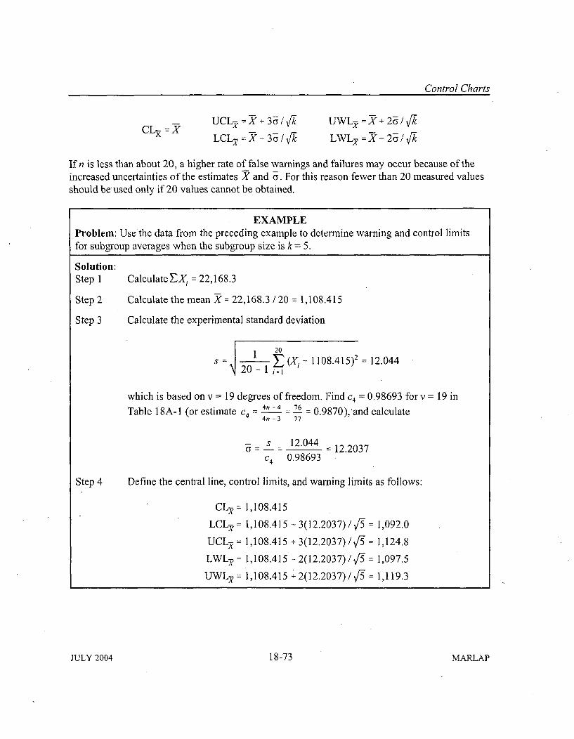
Control Charts

CL2 = XUCL7 X + 3 /

LCL = X- 3a k

UWL~ =XCY//

LWL,7 ~X -2ay

If n is less than about 20, a higher rate of false warnings and failures may occur because of theincreased uncertainties of the estimates X and -. For this reason fewer than 20 measured valuesshould be used only if 20 values cannot be obtained.

EXAMPLEProblem: Use the data from the preceding example to determine warning and control limitsfor subgroup averages when the subgroup size is k = 5.

Solution:Step 1 CalculateEX. = 22,168.3

Step 2 Calculate the mean X = 22,168.3 / 20 = 1,108.415

Step 3 Calculate the experimental standard deviation

S = E0 2 -(X, - 1108.415)2 12.04420 - I j=

which is based on v = 19 degrees of freedom. Find c4 = 0.98693 for v = 19 in

Table 18A- 1 (or estimate c4 4 - = 7 = 0.9870),'and calculate4n - 3 77

- s _ 12.044cy = = - = 12.2037c4 0.98693

Step 4 Define the central line, control limits, and warning limits as follows:

CL2 = 1,108.415

LCL-x = 1,108.415 - 3(12.2037) / x5/ = 1,092.0

UCL)= 1,108.415 + 3(12.2037)/ C5= 1,124.8

LWL -= 1,108.415 - 2(12.2037) / C5 - 1,097.5

UWL) = 1,108.415 + 2(12.2037)/r5 = 1,119.3

JULY 2004 18-73 MARLAP

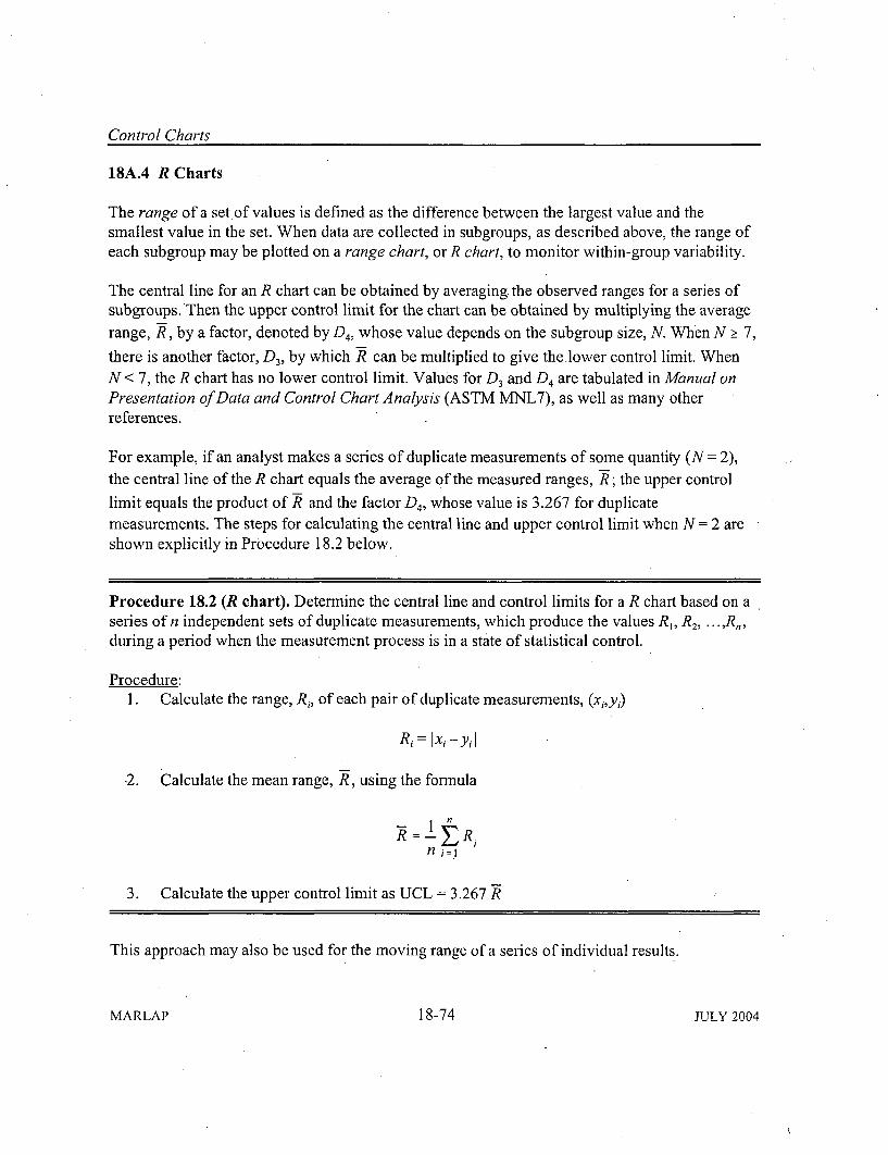
Control Charts

18A.4 R Charts

The range of a set of values is defined as the difference between the largest value and thesmallest value in the set. When data are collected in subgroups, as described above, the range ofeach subgroup may be plotted on a range chart, or R chart, to monitor within-group variability.

The central line for an R chart can be obtained by averaging the observed ranges for a series ofsubgroups. Then the upper control limit for the chart can be obtained by multiplying the averagerange, R, by a factor, denoted by D4, whose value depends on the subgroup size, N. When N >_ 7,there is another factor, D3, by which R can be multiplied to give the lower control limit. WhenN < 7, the R chart has no lower control limit. Values for D3 and D4 are tabulated in Manual onPresentation of Data and Control Chart Analysis (ASTM MNL7), as well as many otherreferences.

For example, if an analyst makes a series of duplicate measurements of some quantity (N = 2),the central line of the R chart equals the average of the measured ranges, R; the upper controllimit equals the product of R and the factor D4, whose value is 3.267 for duplicatemeasurements. The steps for calculating the central line and upper control limit when N = 2 areshown explicitly in Procedure 18.2 below.

Procedure 18.2 (R chart). Determine the central line and control limits for a R chart based on aseries of n independent sets of duplicate measurements, which produce the values R1, R2, ... ,R,during a period when the measurement process is in a state of statistical control.

Procedure:1. Calculate the range, Ri, of each pair of duplicate measurements, (xi,,y)

Ri = Ixi -y I

-2. Calculate the mean range, R, using the formula

n

3. Calculate the upper control limit as UCL = 3.267 R

This approach may also be used for the moving range of a series of individual results.

MARLAP 18-74 JULY 2004

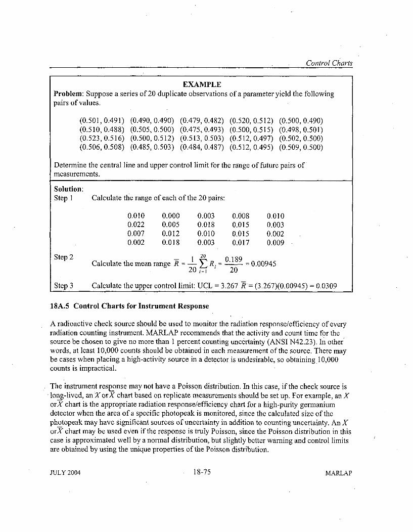
Control Charts

EXAMPLEProblem: Suppose a series of 20 duplicate observations of a parameter yield the followingpairs of values.

(0.501, 0.491) (0.490, 0.490) (0.479, 0.482) (0.520, 0.512) (0.500, 0.490)(0.510, 0.488) (0.505, 0.500) (0.475, 0.493) (0.500, 0.515) (0.498, 0.501)(0.523, 0.516) (0.500, 0.512) (0.513, 0.503) (0.512, 0.497) (0.502, 0.500)(0.506, 0.508) (0.485, 0.503) (0.484, 0.487) (0.512, 0.495) (0.509, 0.500)

Determine the central line and upper control limit for the range of future pairs ofmeasurements.

Solution:Step 1 Calculate the range of each of the 20 pairs:

0.010 0.000 0.003 0.008 0.0100.022 0.005 0.018 0.015 0.0030.007 0.012 0.010 0.015 0.0020.002 0.018 0.003 0.017 0.009

Step 2 - 1 2 0.189Calculate the mean range R E- Ri. - 0.00945

20 j=1 20

Step 3 Calculate the upper control limit: UCL = 3.267 R = (3.267)(0.00945) 0.0309

18A.5 Control Charts for Instrument Response

A radioactive check source should be used to monitor the radiation response/efficiency of everyradiation counting instrument. MARLAP recommends that the activity and count time for thesource be chosen to give no more than 1 percent counting uncertainty (ANSI N42.23). In other/

words, at least 10,000 counts should be obtained in each measurement of the source. There maybe cases when placing a high-activity source in a detector is undesirable, so obtaining 10,000counts is impractical.

The instrument response may not have a Poisson distribution. In this case, if the check source islong-lived, anX orX chart based on replicate measurements should be set up. For example, an XorX chart is the appropriate radiation response/efficiency chart for a high-purity germaniumdetector when the area of a specific photopeak is monitored, since the calculated size of thephotopeak may have significant sources of uncertainty in addition to counting uncertainty. An XorX chart may be used even if the response is truly Poisson, since the Poisson distribution in thiscase is approximated well by a normal distribution, but slightly better warning and control limitsare obtained by using the unique properties of the Poisson distribution.

JULY 2004 18-75 MARLAP

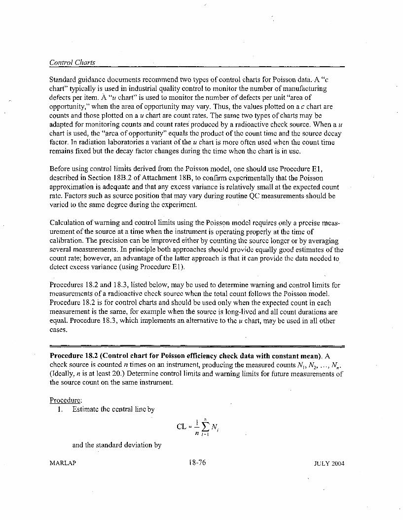
Control Charts

Standard guidance documents recommend two types of control charts for Poisson data. A "cchart" typically is used in industrial quality control to monitor the number of manufacturingdefects per item. A "u chart" is used to monitor the number of defects per unit "area ofopportunity," when the area of opportunity may vary. Thus, the values plotted on a c chart arecounts and those plotted on a u chart are count rates. The same two types of charts may beadapted for monitoring counts and count rates produced by a radioactive check source. When a uchart is used, the "area of opportunity" equals the product of the count time and the source decayfactor. In radiation laboratories a variant of the u chart is more often used when the count timeremains fixed but the decay factor changes during the time when the chart is in use.

Before using control limits derived from the Poisson model, one should use Procedure E 1,described in Section 188.2 of Attachment 18B, to confirm experimentally that the Poissonapproximation is adequate and that any excess variance is relatively small at the expected countrate. Factors such as source position that may vary during routine QC measurements should bevaried to the same degree during the experiment.

Calculation of warning and control limits using the Poisson model requires only a precise meas-urement of the source at a time when the instrument is operating properly at the time ofcalibration. The precision can; be improved either by counting the source longer or by averagingseveral measurements. In principle both approaches should provide equally good estimates of thecount rate; however, an advantage of the latter approach is that it can provide the data needed todetect excess variance (using Procedure E l).

Procedures 18.2 and 18.3, listed below, may be used to determine warning and control limits formeasurements of a radioactive check source when the total count follows the Poisson model.Procedure 18.2 is for control charts and should be used only when the expected count in eachmeasurement is the same, for example when the source is long-lived and all count durations areequal. Procedure 18.3, which implements an alternative to the u chart, may be used in all othercases.

Procedure 18.2 (Control chart for Poisson efficiency check data with constant mean). Acheck source is counted n times on an instrument, producing the measured counts N,, N 2, ... , N,.(Ideally, n is at least 20.) Determine control limits and warning limits for future measurements ofthe source count on the same instrument.

Procedure:I. Estimate the central line by

CL=Z N

and the standard deviation by

MARLAP 18-76 JULY 2004

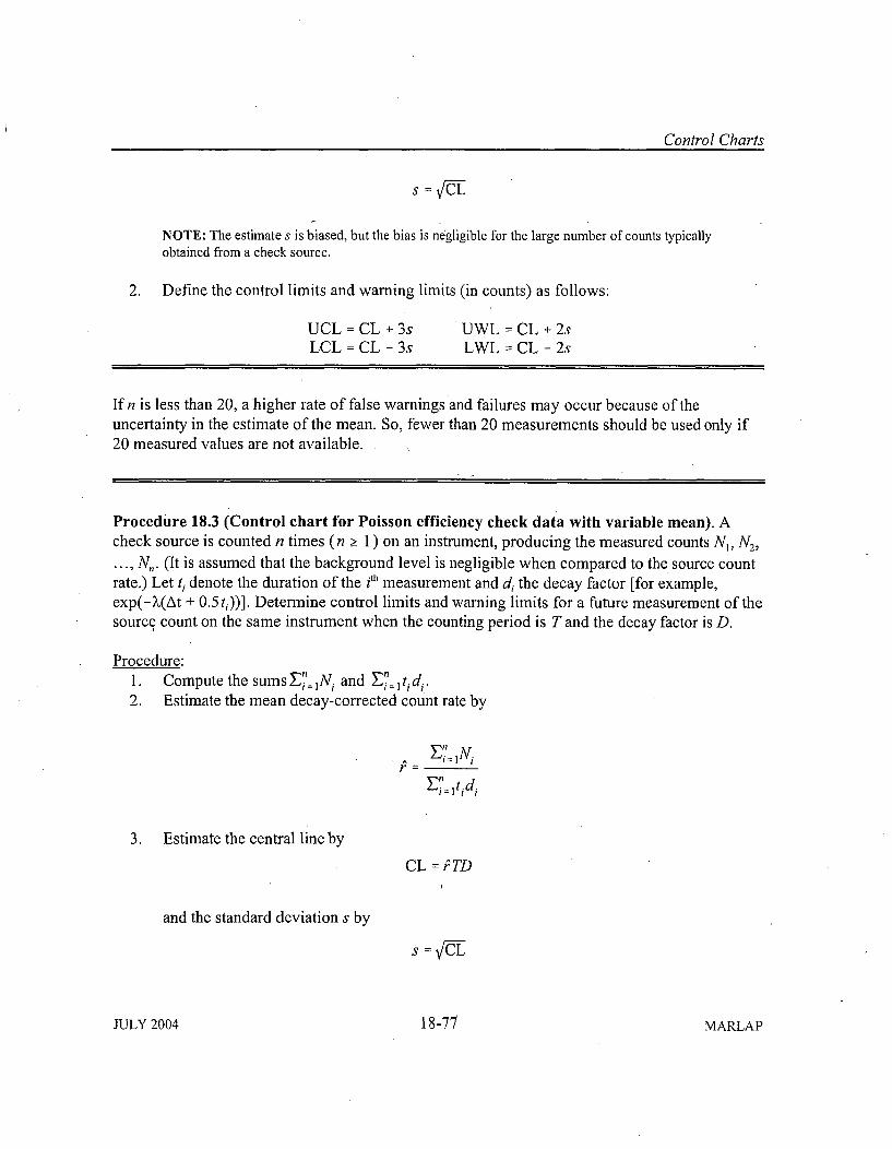
Control Charts

s=f~i

NOTE: The estimate s is biased, but the bias is negligible for the large number of counts typicallyobtained from a check source.

2. Define the control limits and warning limits (in counts) as follows:

UCL = CL + 3sLCL = CL - 3s

UWL = CL + 2sLWL = CL - 2s

If n is less than 20, a higher rate of false warnings and failures may occur because of theuncertainty in the estimate of the mean. So, fewer than 20 measurements should be used only if20 measured values are not available.

Procedure 18.3 (Control chart for Poisson efficiency check data with variable mean). Acheck source is counted n times (n Ž_ 1 ) on an instrument, producing the measured counts N,, NV,,... , Nn. (It is assumed that the background level is negligible when compared to the source countrate.) Let tj denote the duration of the ith measurement and di the decay factor [for example,exp(-X(At + 0.5 ti))]. Determine control limits and warning limits for a future measurement of thesource count on the same instrument when the counting period is T and the decay factor is D.

Procedure: SUM Fn= E n, ti di.1.* Compute the sums•i ~ Ni and i i,2. Estimate the mean decay-corrected count rate by

r = t

3. Estimate the central line by

CL = PTD

and the standard deviation s by

s=CVL

JULY 2004 18-71 MARLAP

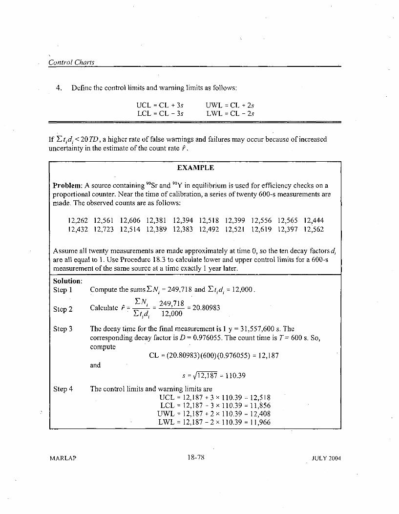
Control Charts

4. Define the control limits and warning limits as follows:

UCL =CL + 3s UWL = CL + 2sLCL = CL - 3s LWL = CL - 2s

If t, id < 20 TD, a higher rate of false warnings and failures may occur because of increaseduncertainty in the estimate of the count rate P.

EXAMPLE

Problem: A source containing 9"Sr and 90Y in equilibrium is used for efficiency checks on aproportional counter. Near the time of calibration, a series of twenty 600-s measurements aremade. The observed counts are as follows:

12,262 12,561 12,606 12,381 12,394 12,518 12,399 12,556 12,565 12,44412,432 12,723 12,514 12,389 12,383 12,492 12,521 12,619 12,397 12,562

Assume all twenty measurements are made approximately at time 0, so the ten decay factors diare all equal to 1. Use Procedure 18.3 to calculate lower and upper control limits for a 600-smeasurement of the same source at a time exactly 1 year later.

Solution:Step 1 Compute the sumsEN, = 249,718 and Et,id = 12,000.

__Ni _ 249,718 = 20.80983Step 2 Calculate r - =-t•0.8 12,00

>1tid1 12,000

Step 3 The decay time for the final measurement is 1 y = 31,557,600 s. Thecorresponding decay factor is D = 0.976055. The count time is T= 600 s. So,compute

CL = (20.80983) (600) (0.976055) = 12,187and

s 12,187 = 110.39

Step 4 The control limits and warning limits areUCL = 12,187 + 3 x 110.39 = 12,518LCL = 12,187 -3 x 110.39 = 11,856

UWL = 12,187 + 2 x 110.39 = 12,408LWL = 12,187 - 2 x 110.39 = 11,966

MARLAP 18-78 JULY 2004

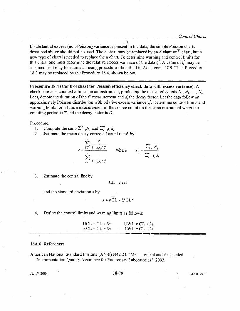
Control Charts

If substantial excess (non-Poisson) variance is present in the data, the simple Poisson chartsdescribed above should not be used. The c chart may be replaced by an X chart orX chart, but anew type of chart is needed to replace the u chart. To determine warning and control limits forthis chart, one must determine the relative excess variance of the data 42. A value of 2 may beassumed or it may be estimated using procedures described in Attachment 18B. Then Procedure18.3 may be replaced by the Procedure 18.4, shown below.

Procedure 18.4 (Control chart for Poisson efficiency check data with excess variance). Acheck source is counted n times on an instrument, producing the measured counts N,, N2, ... , N,.Let ti denote the duration of the ith measurement and d, the decay factor. Let the data follow anapproximately Poisson distribution with relative excess variance.4'. Determine control limits andwarning limits for a future measurement of the source count on the same instrument when thecounting period is T and the decay factor is D.

Procedure:1. Compute the sums Ej= jN, and E=, Itidi2. --Estimate the mean decay-corrected count rate P by

n"Ali

'I1 +rot.d 2 where r0 N1.n Ell

E 1 I i-l t i4

j =1 I + rotidjý2

3. Estimate the central line byCL =PTD

and the standard deviation s by

s VCL + 42 CL 2

4. Define the control limits and warning limits as follows:

UCL = CL + 3s UWL = CL + 2sLCL = CL - 3s LWL = CL - 2s

18A.6 References

American National Standard Institute (ANSI) N42.23. "Measurement and AssociatedInstrumentation Quality Assurance for Radioassay Laboratories." 2003.

JULY 2004 18-79 MARLAP

Control Charts

American Society for Testing and Materials (ASTM) D6299. Standard Practice for ApplyingStatistical Quality Assurance Techniques to Evaluate Analytical Measurement SystemPerformance, 2000, West Conshohocken, Pennsylvania.

American Society for Testing and Materials (ASTM) E882, Standard Guide for Accountabilityand Quality Control in the Chemical Analysis Laboratory, 1998, West Conshohocken,Pennsylvania.

American Society for Testing and Materials (ASTM) MNL 7, Manual on Presentation of Dataand Control Chart Analysis ASTM Manual Series, 7th Edition, 2002

National Bureau of Standards (NBS). 1964. Handbook of Mathematical Functions. M.Abramowitz and Stegun, I., Editors.

MARLAP 18-80 JULY 2004

ATTACHMENT 18BStatistical Tests for QC Results

18B.1 Introduction

Attachment 18A describes several types of control charts that may be used for statistical qualitycontrol in the laboratory. This attachment describes additional statistical methods that may beused, where appropriate, to test the performance of measurement results from blank, replicate,LCS, spikes, CRM, yield-monitor, background, efficiency, calibration, or peak resolution results,with special emphasis on instrumentation results.

18B.2 Tests for Excess Variance in the Instrument Response

As noted in Chapter 19, the counting uncertainty given by the Poisson approximation does notdescribe the total variability in a counting measurement. A number of factors may generate asmall excess component of variance. When a large number of counts are obtained in the meas-urement, the relative magnitude of the Poisson variance is small; so, the excess component maydominate.

Regardless of whether replication or the Poisson approximation is used to estimate countinguncertainties, MARLAP recommends that a series of check source measurements be made oneach instrument periodically to test for excess variance. Procedure E 1, which is presented below,may be used to evaluate the measurement results. To check the stability of the instrument itself,one should perform the measurements while holding constant any controllable factors, such assource position, that might increase the variance. To check the variance when such factors are notconstant, one may use Procedure E l but vary the factors randomly for each measurement.

Assume n measurements of the source produce the counts N1 , N2, ... , N,. If the expected countfor each measurement is at least 20, so that the Poisson distribution is approximated by a normaldistribution, and if the average decay-corrected count rate P is determined with adequateprecision, then the quantity

X2 _ E ti (18.10)

where t1 and di are the count time and source decay factor for the ith measurement, respectively,should be distributed approximately as chi-square with n - I degrees of freedom.5 The precision

5 If r denotes the true mean decay-corrected count rate, then under the null hypothesis each measured count rateNi / tidi is approximately normal with mean r and variance r / tid,, and the least-squares estimator for r isP ENý / Etidi. So, the sum E(N] / tiýd_ -p) 2 / (r / tid) is approximately chi-square with n - I degrees of freedom.

JULY 2004 18-81 MARLAP

Statistical Tests for QC Results

of the estimate P should be adequate for the test as long as the expected count for each measure-ment is at least 20. Since a check source is involved, the expected count is usually much greaterthan 20.

Procedure El. The x- (chi-square) analysis can be used to determine whether a series ofmeasurements of a check source provide evidence of variance in excess of the Poisson countingvariance. Let Ni denote the count observed in the ith measurement. Let wi = tfid, where ti denotesthe count time and di denotes the source decay factor (if relevant). If all the values w; are equal,one may use w= 1 instead for all i. It is assumed either that the background count rate isnegligible or that the decay factors are all nearly equal, so that the expected count in eachmeasurement is proportional to wi.6 The procedure tests the null hypothesis that the totalmeasurement variance is the Poisson counting variance.

Procedure:1. Choose the significance level a2. Calculate the sums 'i=1 N1 and Z7=,w,3. Estimate the mean decay-corrected count rate by

,7N (18.11),i =]1Wi

4. Calculate the chi-square statistic as follows:

.. (18.12)Fi1Wi

5. Determine the quantile X, _J(n - 1) (see Table G.3 in Appendix G). Reject the nullhypothesis if and only if the calculated value of X2 is greater than1 _,(n -1). In this caseconclude that the variance is greater than predicted by the Poisson model.

If P is determined accurately, the true mean count rate r may be replaced in the formula by its estimated value P toobtain the formula that appears in the text. If all the products tidi are equal, they cancel out of the sum, whichbecomes E(N, - N) 2 /TI, as described by Evans (1955), Goldin (1984), and Knoll (1989).

6 The expected gross count for the iph measurement equals RB ti + r wi, where r is the mean net count rate at time 0.The expected count is proportional to wi if RB =0, or if all the decay factors are equal so that ti,- w,.

MARLAP 18-82 JULY 2004

Statistical Tests for QC Results

EXAMPLE

Problem: A long-lived source is counted n = 20 times in a gross radiation detector and theduration of each measurement is 300 s. The following total counts are measured:

11,189 11,105 11,183 10,910 10,998 11,137 11,144 10,751 11,128 11,03711,205 11,040 11,257 11,176 10,976 10,998 11,023 11,199 11,078 11,149

Are these data consistent with the assumption that the measurement variance is no greater thanpredicted by the Poisson model? Use 5 percent as the significance level.

Solution:Step 1 The significance level is specified to be a,= 0.05

Step 2 Since the source is long-lived and all the count times are equal, let wi = 1 foreach i. Calculate EN, = 221,683 and Ewi 20

Step 3 Calculate the mean count rate P 221,683 /20 = 11,084.15

Step 4 Calculate the chi-square statistic

.. .. Fw 1.- 8 (N.- 11,084.15)2 =24.87r i t= wi w 11,084.15 =

Step 5 The number of degrees of freedom is 20 - 1 = 19. According to Table G.3, the0.95-quantile for a chi-square distribution with 19 degrees of freedom is 30.14.Since 24.87 < 30.14, do not reject the null hypothesis. The data are consistentwith the assumption of Poisson counting statistics at the 5 percent significancelevel.

A two-sided version of Procedure E l may also be used to test whether the measurement varianceis either greater than or less than predicted by the Poisson model. Step 5 must be changed so thatthe null hypothesis is rejected if the value of the test statistic z2 does not lie between the two• -- 2

quantiles x•12(n - 1) and X1 -, 2 (n - 1).

A chi-square test may require many measurements or long count times to detect a small excessvariance component. When all measurements have the same expected count R, the detection limitfor the relative excess variance, or its minimum detectable value, is equal to

(2

1 (18,13)X",2(n - 1

JULY 2004 18-83 MARLAP

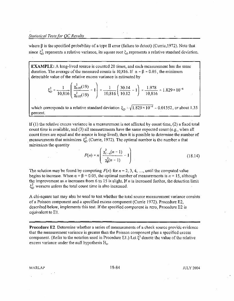
Statistical Tests for QC Results

where P is the specified probability of a type II error (failure to detect) (Currie, 1972). Note that

since ý2 represents a relative variance, its square root ýD represents a relative standard deviation.

EXAMPLE: A long-lived source is counted 20 times, and each measurement has the sameduration. The average of the measured counts is 10,816. If a = P = 0.05, the minimumdetectable value of the relative excess variance is estimated by

2 _ 1 , (95(19) ) = 1 30.14 1 1.978 _1.829x10-4

10,816 2 10,816 10.12 10,8160. 05(19)

which corresponds to a relative standard deviation 4D = 1.829x 10-4 = 0.01352, or about 1.35percent.

If (1) the relative excess variance in a measurement is not affected by count time, (2) a fixed totalcount time is available, and (3) all measurements have the same expected count (e.g., when allcount times are equal and the source is long-lived), then it is possible to determine the number ofmeasurements that minimizes {2 (Currie, 1972). The optimal number is the number n thatminimizes the quantity

F(n) =n nx-(n 1J (18.14)

The solution may be found by, computing F(n) for n = 2, 3, 4, ... , until the computed valuebegins to increase. When a = 0 = 0.05, the optimal number of measurements is n = 15, althoughthe improvement as n increases from 6 to 15 is slight. If n is increased further, the detection limit

2 worsens unless the total count time is also increased.

A chi-square test may also be used to test whether the total source measurement variance consistsof a Poisson component and a specified excess component (Currie 1972). Procedure E2,described below, implements this test. If the specified component is zero, Procedure E2 isequivalent to E 1.

Procedure E2. Determine whether a series of measurements of a check source provide evidencethat the measurement variance is greater than the Poisson component plus a specified excesscomponent. (Refer to the notation used in Procedure El.) Let ý2 denote the value of the relativeexcess variance under the null hypothesis H0.

MARLAP 18-84 JULY 2004

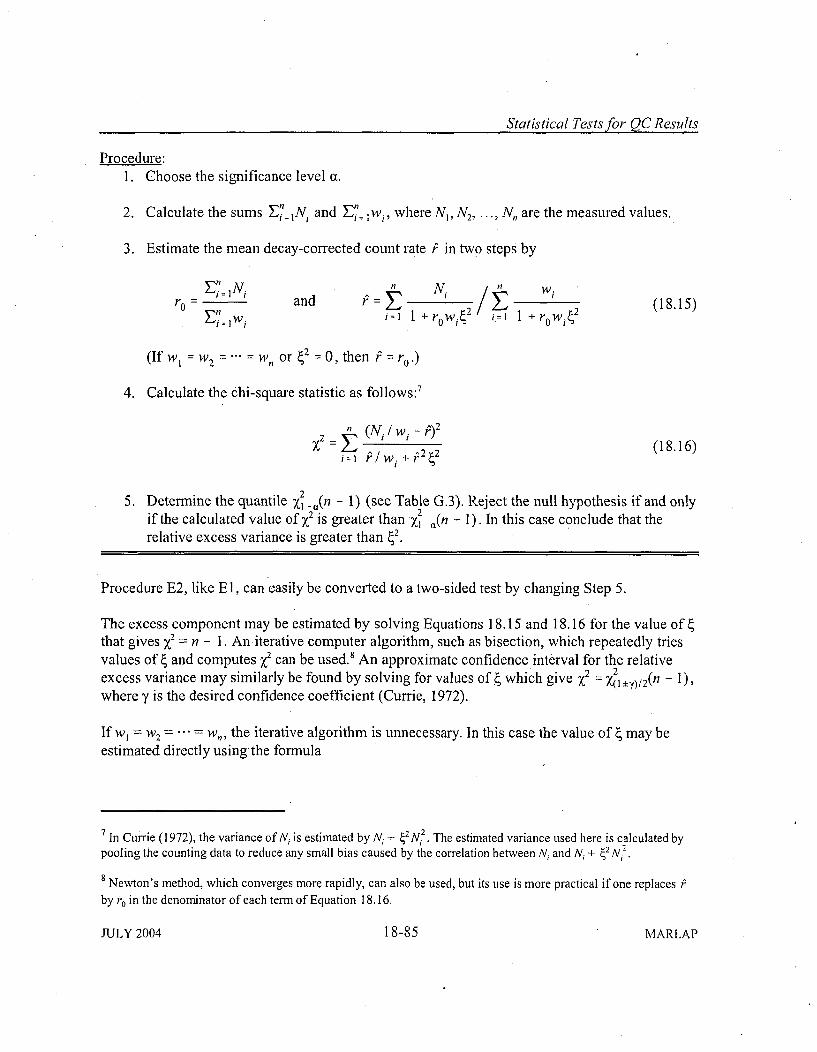
Statistical Tests for QC Results

Procedure:1. Choose the significance level a.

2. Calculate the sums Ei"=,A and E".Z Iwi, where N,, N 2,..., N, are the measured values.

3. Estimate the mean decay-corrected count rate P• in two steps by

E n=l n n wiro- i and N= (18.15)

i=i i=1 1 +r oW i4=2 1 + r wi•2

(If w =w2 . w or 2 -0, then P = r..)

4. Calculate the chi-square statistic as follows:7

X2 = n (N./wi-P)2

E ,=242 (18.16)i=1 •/Wi + •

le2

5. Determine the quantile X, _n - 1) (see Table G.3). Reject the null hypothesis if and only2if the calculated value of x2 is greater than X,- _(n - 1). In this case conclude that therelative excess variance is greater than 42.

Procedure E2, like El, can easily be converted to a two-sided test by changing Step 5.

The excess component may be estimated by solving Equations 18.15 and 18.16 for the value ofthat gives x2 = n - 1. Aniterative computer algorithm, such as bisection, which repeatedly triesvalues of 4 and computes Z2 can be used.8 An approximate confidence interval for the relativeexcess variance may similarly be found by solving for values of 4 which give ±2 2exces whch gve x= X(I+±/)/ 2(f/ - 1),

where y is the desired confidence coefficient (Currie, 1972).

If w1 = W2 ... w,, the iterative algorithm is unnecessary. In this case the value of 4 may beestimated directly using the formula

7 In Currie (1972), the variance ofN, is estimated byN, + 42N 2 . The estimated variance used here is calculated bypooling the counting data to reduce any small bias caused by the correlation between N, and N, + ý-2N7.

8 Newton's method, which converges more rapidly, can also be used, but its use is more practical if one replaces P

by k0 in the denominator of each term of Equation 18.16.

JULY 2004 18-85 MARLAP

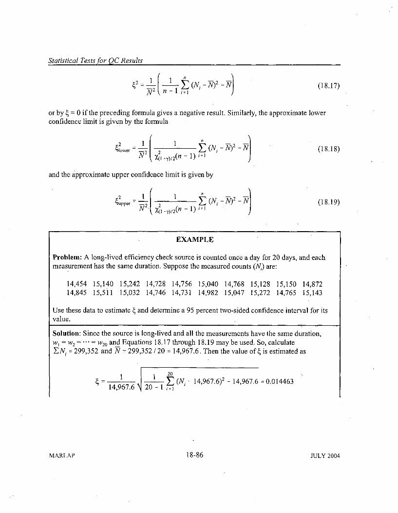
Statistical Tests for QC Results

2( -A - (18.17)

or by 4 = 0 if the preceding formula gives a negative result. Similarly, the approximate lowerconfidence limit is given by the formula

2 n2412ower 1 -1 (Ný - TV)2-NJ (18.18)X(2 ,1)/2(n -1)i ,

and the approximate upper confidence limit is given by

2upper l 1) Z(N -2)2-N) (18.19)

EXAMPLE

Problem: A long-lived efficiency check source is counted once a day for 20 days, and eachmeasurement has the same duration. Suppose the measured counts (N,) are:

14,454 15,140 15,242 14,728 14,756 15,040 14,768 15,128 15,150 14,87214,845 15,511 15,032 14,746 14,731 14,982 15,047 15,272 14,765 15,143

Use these data to estimate ý and determine a 95 percent two-sided confidence interval for itsvalue.

Solution: Since the source is long-lived and all the measurements have the same duration,w1 = W2 =.... w20 and Equations 18.17 through 18.19 may be used. So, calculateEN, = 299,352 and N7V 299,352 / 20 = 14,967.6. Then the value of is estimated as

201 (N, - 14,967.6)2 - 14,967.6 = 0.014463{-14,967.6 20 -1 io=

MARLAP 18-86 JULY 2004

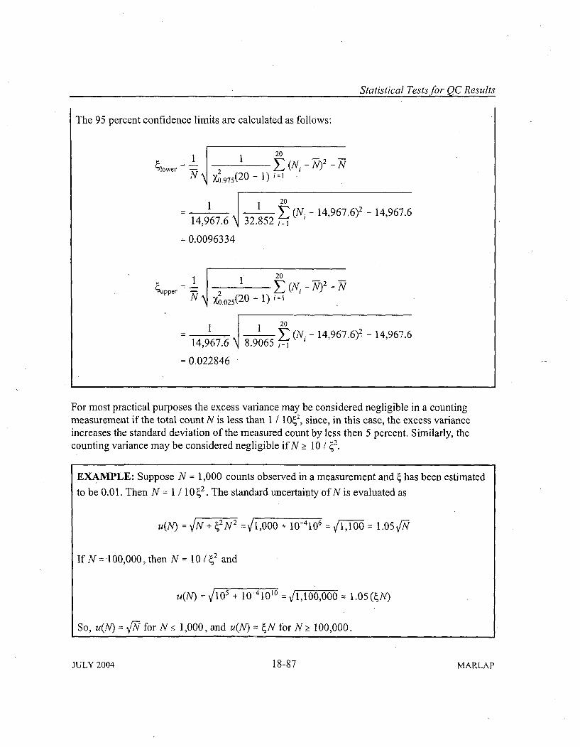
Statistical Tests for QC Results

The 95 percent confidence limits are calculated as follows:

1 2 0 2 - T V

41ower = 1: I__2 -(N TV) 2

N (0.975(20 - 1) i=i

S14, . 3 2 E (Ni - 14,967.6)2 - 14,967.614,967.6 32.852 =

= 0.0096334

1 I 1 20 2 TV -4uppor-= 2 E-]- VuXO.025(

2 0 1)i=

_14 1 8.9N6- 14,967.6)ý - 14,967.614,967.6 8.9065 1=1

- 0.022846

For most practical purposes the excess variance may be considered negligible in a countingmeasurement if the total count N is less than 1 / 10I 0, since, in this case, the excess varianceincreases the standard deviation of the measured count by less then 5 percent. Similarly, thecounting variance may be considered negligible if N 2! 10 / 42.

EXAMPLE: Suppose N = 1,000 counts observed in a measurement and 4 has been estimated

to be 0.01. Then N = I / 10ý2. The standard uncertainty of N is evaluated as

U(N) = N+- ý 2 N 2 = 1,000 + 10-4106 = 1,100 1.05•/-

If N = 100,000, then N = 10 / 2 and

u(N) = V105

+ 10-41010 = 1,100,000 1.05(ýN)

So, u(N) = CN for N•_ 1,000, and u(N) z 4N for N >_ 100,000.

JULY 2004 18-87 MARLAP

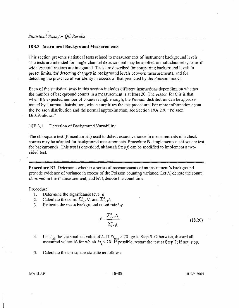
Statistical Tests for QC Results

18B.3 Instrument Background Measurements

This section presents statistical tests related to measurements of instrument background levels.The tests are intended for single-channel detectors but may be applied to multichannel systems ifwide spectral regions are integrated. Tests are described for comparing background levels topreset limits, for detecting changes in background levels between measurements, and fordetecting the presence of variability in excess of that predicted by the Poisson model.

Each of the statistical tests in this section includes different instructions depending on whetherthe number of background counts in a measurement is at least 20. The reason for this is thatwhen the expected number of counts is high enough, the Poisson distribution can be approxi-mated by a normal distribution, which simplifies the test procedure. For more information aboutthe Poisson distribution and the normal approximation, see Section 19A.2.9, "PoissonDistributions."

18B.3.1 Detection of Background Variability

The chi-square test (Procedure El) used to detect excess variance in measurements of a checksource may be adapted for background measurements. Procedure B 1 implements a chi-square testfor backgrounds. This test is one-sided, although Step.6 can be modified to implement a two-sided test.

Procedure B1. Determine whether a series of measurements of an instrument's backgroundprovide evidence of variance in excess of the Poisson counting variance. Let N, denote the countobserved in the ith measurement, and let ti denote the count time.

Procedure:1. Determine the significance level a2. Calculate the sums E"= ANi and E"=, ti3. Estimate the mean background count rate by

El% (18.20)•i = ti

4. Let tmin be the smallest value of ti. If 'tmin _> 20, go to Step 5. Otherwise, discard allmeasured values Ni for which Pti < 20. If possible, restart the test at Step 2; if not, stop.

5. Calculate the chi-square statistic as follows:

MARLAP 18-88 JULY 2004

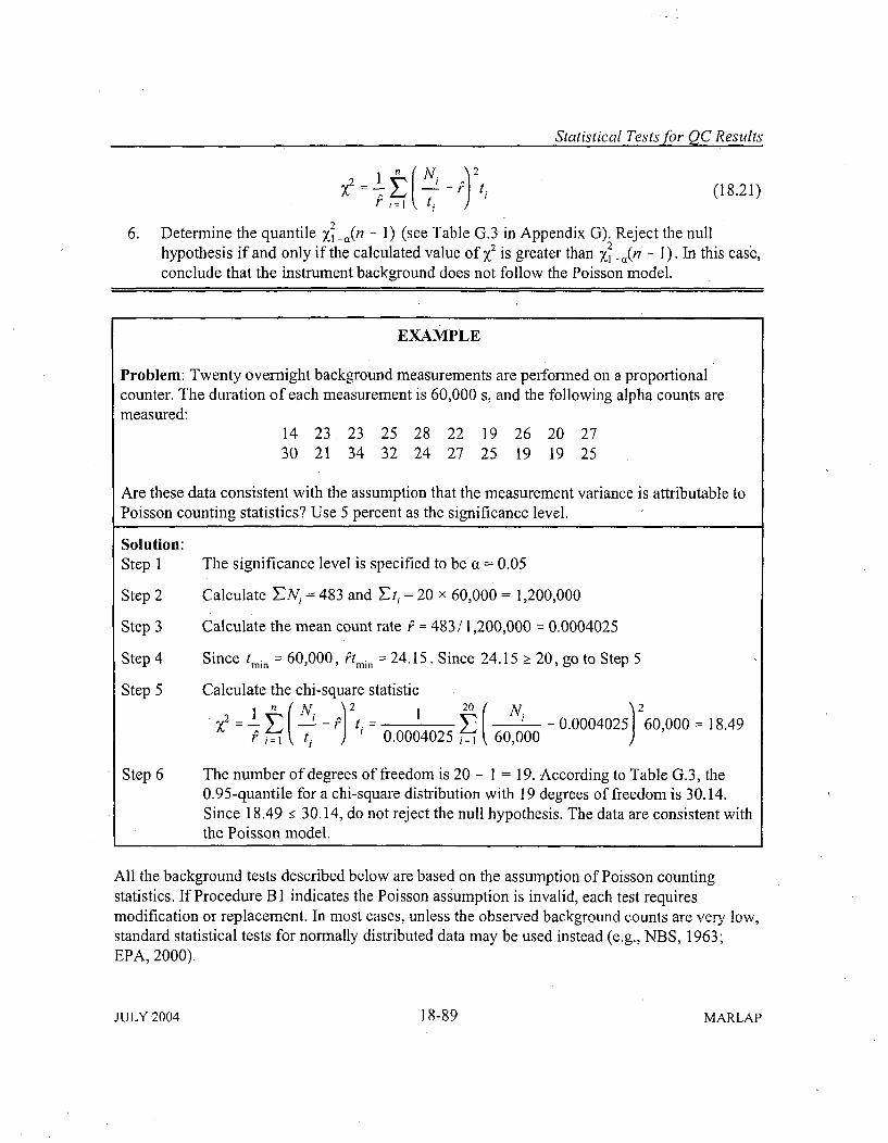
Statistical Tests for QC Results

X2 (N. _-) ti (18.21)

6. Determine the quantile X, _ (n - 1) (see Table G.3 in Appendix G). Reject the nullhypothesis if and only if the calculated value of x is greater than 2• - a(n - 1). In this case,conclude that the instrument background does not follow the Poisson model.

EXAMPLE

Problem: Twenty overnight background measurements are performed on a proportionalcounter. The duration of each measurement is 60,000 s, and the following alpha counts aremeasured:

14 23 23 25 28 22 19 26 20 2730 21 34 32 24 27 25 19 19 25

Are these data consistent with the assumption that the measurement variance is attributable toPoisson counting statistics? Use 5 percent as the significance level.Solution:

Step 1 The significance level is specified to be a 0.05

Step 2 Calculate ENi = 483 and Zti = 20 x 60,000 = 1,200,000

Step 3 Calculate the mean count rate P = 483 / 1,200,000 = 0.0004025

Step 4 Since tmin = 60,000, Ptmin = 24.15. Since 24.15 >_ 20, go to Step 5

Step 5 Calculate the chi-square statistic

S ( - t - 0.0004025 60,000 18.49= t0.0004025 . 60,000

Step 6 The number of degrees of freedom is 20 - 1 = 19. According to Table G.3, the0.95-quantile for a chi-square distribution with 19 degrees of freedom is 30.14.Since 18.49 :< 30.14, do not reject the null hypothesis. The data are consistent withthe Poisson model.

All the background tests described below are based on the assumption of Poisson countingstatistics. If Procedure B I indicates the Poisson assumption is invalid, each test requiresmodification or replacement. In most cases, unless the observed background counts are very low,standard statistical tests for normally distributed data may be used instead (e.g., NBS, 1963;EPA, 2000).

JULY 2004 18-89 MARLAP

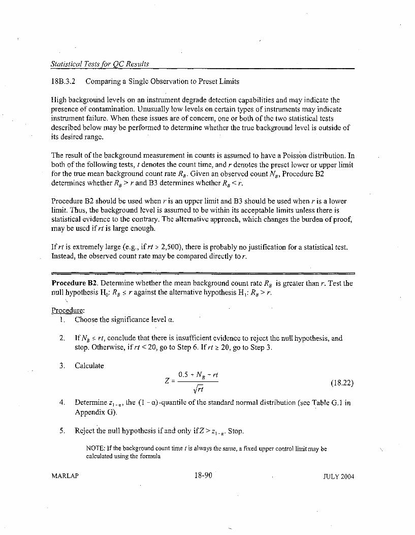
Statistical Tests for QC Results

188.3.2 Comparing a Single Observation to Preset Limits

High background levels on an instrument degrade detection capabilities and may indicate thepresence of contamination. Unusually low levels on certain types of instruments may indicateinstrument failure. When these issues are of concern, one or both of the two statistical testsdescribed below may be performed to determine whether the true background level is outside ofits desired range.

The result of the background measurement in counts is assumed to have a Poisson distribution. Inboth of the following tests, t denotes the count time, and r denotes the preset lower or upper limitfor the true mean background count rate RB. Given an observed count NB, Procedure B2determines whether RB > r and B3 determines whether RB < r.

Procedure B2 should be used when r is an upper limit and B3 should be used when r is a lowerlimit. Thus, the background level is assumed to be within its acceptable limits unless there isstatistical evidence to the contrary. The alternative approach, which changes the burden of proof,may be used if rt is large enough.

If rt is extremely large (e.g., if rt Žo 2,500), there is probably no justification for a statistical test.Instead, the observed count rate may be compared directly to r.

Procedure B2. Determine whether the mean background count rate RB is greater than r. Test thenull hypothesis H0: RB _• r against the alternative hypothesis H:RB > r.

Procedure:1. Choose the significance level a.

2. If NB _ rt, conclude that there is insufficient evidence to reject the null hypothesis, andstop. Otherwise, if rt < 20, go to Step 6. If rt Ž_ 20, go to Step 3.

3. Calculate0.5 +NB - rt

Z- = (18.22)

4. Determine zI -, the (I -a)-quantile of the standard normal distribution (see Table G. I inAppendix G).

5. Reject the null hypothesis if and only ifZ > z,. Stop.

NOTE: If the background count time I is always the same, a fixed upper control limit may becalculated using the formula

MARLAP 18-90 JULY 2004

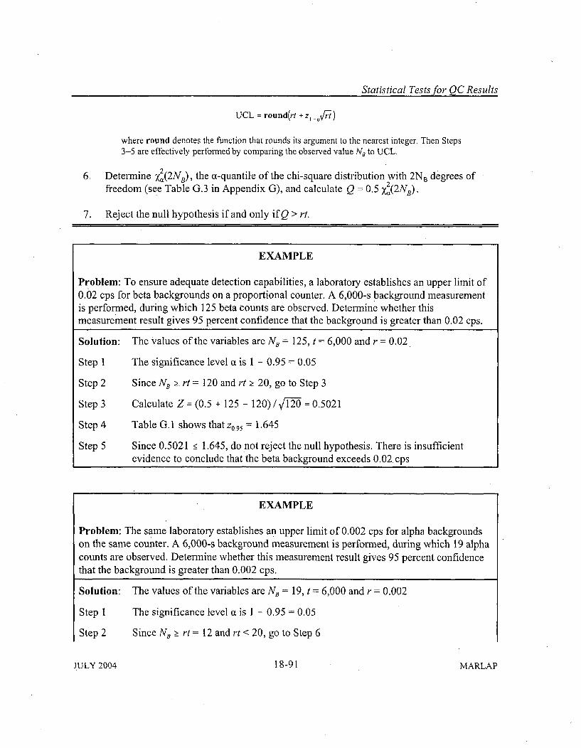
Statistical Tests for QC Results

UCL = round(rt + z, _V17 )

where round denotes the function that rounds its argument to the nearest integer, Then Steps3-5 are effectively performed by comparing the observed value N8 to UCL.

6. Determine 2 (2NB), the a-quantile of the chi-square distribution with 2NB degrees offreedom (see Table G.3 in Appendix G), and calculate Q = 0.5 X.(2NB).

7. Reject the null hypothesis if and only ifQ > rt.

EXAMPLE

Problem: To ensure adequate detection capabilities, a laboratory establishes an upper limit of0.02 cps for beta backgrounds on a proportional counter. A 6,000-s background measurementis performed, during which 125 beta counts are observed. Determine whether thismeasurement result gives 95 percent confidence that the background is greater than 0.02 cps.

Solution: The Values of the variables are N, = 125, t = 6,000 and r = 0.02

Step I The significance level a is I - 0.95 = 0.05

Step 2 Since N 8. Ž rt = 120 and rt >_ 20, go to Step 3

Step 3 Calculate Z = (0.5 + 125 - 120)/yT2 = 0.5021

Step 4 Table G.1 shows that z0.95 = 1.645

Step 5 Since 0.5021 < 1.645, do not reject the null hypothesis. There is insufficientevidence to conclude that the beta background exceeds 0.02 cps

EXAMPLE

Problem: The same laboratory establishes an upper limit of 0.002 cps for alpha backgroundson the same counter. A 6,000-s background measurement is performed, during which 19 alphacounts are observed. Determine whether this measurement result gives 95 percent confidencethat the background is greater than 0.002 cps.

Solution: The values of the variables are N8 = 19, t = 6,000 and r = 0.002

Step 1 The significance level a is 1 - 0.95 = 0.05

Step 2 Since NB, > rt = 12 and rt < 20, go to Step 6

JULY 2004 18-91 MARLAP

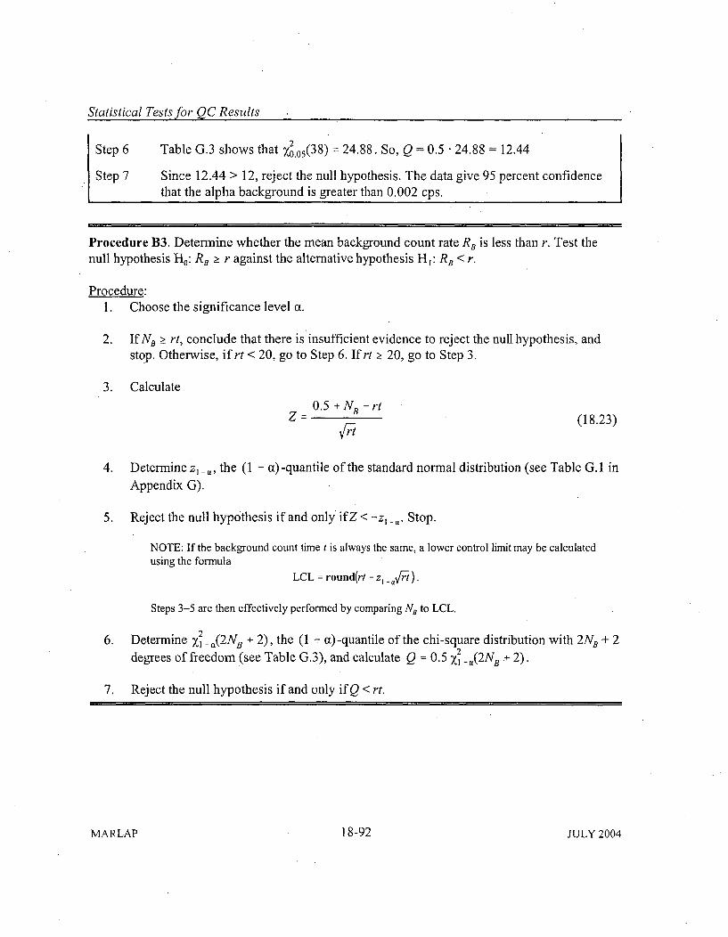
Statistical Tests for QC Results

Step 6 Table G.3 shows that XO,05(38) = 24.88. So, Q = 0.5 • 24.88 = 12.44

Step 7 Since 12.44 > 12, reject the null hypothesis. The data give 95 percent confidencethat the alpha background is greater than 0.002 cps.

Procedure B3. Determine whether the mean background count rate RB is less than r. Test thenull hypothesis H0: RB Ž-- r against the alternative hypothesis H 1: R, < r.

Procedure:1. Choose the significance level a.

2. If NB >_ rt, conclude that there is insufficient evidence to reject the null hypothesis, andstop. Otherwise, if rt < 20, go to Step 6. If rt Ž_ 20, go to Step 3.

3. Calculate

0.5 + NB - rtZ = (18.23)

4. Determine z, , the (1 - a) -quantile of the standard normal distribution (see Table G. 1 in

Appendix G).

5. Reject the null hypothesis if and only ifZ < -z,_,. Stop.

NOTE: If the background count time t is always the same, a lower control limit may be calculatedusing the formula

LCL = round(rt - zI _,F).

Steps 3-5 are then effectively performed by comparing NB to LCL.

6. Determine X,_ a(2NB + 2), the (1 - a)-quantile of the chi-square distribution with 2NB + 22

degrees of freedom (see Table G.3), and calculate Q = 0.5 X, _ (2NB + 2).

7. Reject the null hypothesis if and only if Q < rt.

MARLAP 18-92 JULY 2004

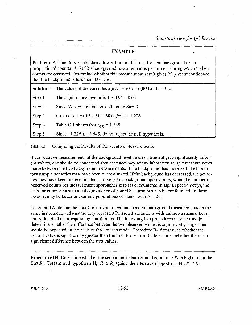
Statistical Tests for QC Results

EXAMPLE

Problem: A laboratory establishes a lower limit of 0.01 cps for beta backgrounds on aproportional counter. A 6,000-s background measurement is performed, during which 50 betacounts are observed. Determine whether this measurement result gives 95 percent confidencethat the background is less than 0.01 cps.

Solution: The values of the variables are NB = 50, t = 6,000 and r =0.01

Step 1 The significance level a is 1 - 0.95 = 0.05

Step 2 Since NB :- rt = 60 and rt Ž_ 20, go to Step 3

Step 3 Calculate Z = (0.5 + 50 - 60) / V = -1.226

Step 4 Table G. 1 shows that z0.95 = 1.645

Step 5 Since - 1.226 Ž_ - 1.645, do not reject the null hypothesis.

18B.3.3 Comparing the Results of Consecutive Measurements

If consecutive measurements of the background level on an instrument give significantly differ-ent values, one should be concerned about the accuracy of any laboratory sample measurementsmade between the two background measurements. If the background has increased, the labora-tory sample activities may have been overestimated. If the background has decreased, the activi-ties may have been underestimated. For very low background applications, when the number ofobserved counts per measurement approaches zero (as encountered in alpha spectrometry), thetests for comparing statistical equivalence of paired backgrounds can be confounded. In thesecases, it may be better to examine populations of blanks with N Ž> 20.

Let N, and N 2 denote the counts observed in two independent background measurements on thesame instrument, and assume they represent Poisson distributions with unknown means. Let tjand t2 denote the corresponding count times. The following two procedures may be used todetermine whether the difference between the two observed values is significantly larger thanwould be expected on the basis of the Poisson model. Procedure B4 determines whether thesecond value is significantly greater than the first. Procedure B5 determines whether there is asignificant difference between the two values.

Procedure B4. Determine whether the second mean background count rate R 2 is higher than thefirst R,. Test the null hypothesis I-J: R, >] R, against the alternative hypothesis H,: R < R2.

JULY 2004 18-93 MARLAP

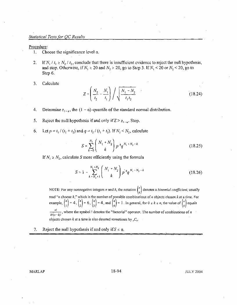
Statistical Tests for QC Results

Procedure:1. Choose the significance level a.

2. If N, / t, >Ž N2 / t 2, conclude that there is insufficient evidence to reject the null hypothesis,and stop. Otherwise, if N, > 20 and N2 >- 20, go to Step 3. IfN, < 20 or N2 < 20, go toStep 6.

3. Calculate

Z= 2_(18.24)1 2 t It l t2

4. Determine zl I, the (1 - a)-quantile of the standard normal distribution.

5. Reject the null hypothesis if and only ifZ > z,. Stop.

6. Letp = t, / (t, + t2) and q = t2 / (0 + t2). IfN, < N2, calculate

S N= 1 N, + N2 kqN, +N2- kS= o E P q (18.25)

If N, Ž N2, calculate S more efficiently using the formula

N, +N2 JN1 + N2 k M+N2 -S= I - ( pkqN+U2 k (18.26)

ks=N + k

NOTE: For any nonnegative integers n and k, the notation (n) denotes a binomial coefficient, usually

read "n choose k," which is the number of ossible combinations ofn objects chosen k at a time. Forexample, (4)= 4, (4) 6, (4)= 4, and (4) = 1. In general, for 0• k • n, the value of (n) equals

n! where the symbol denotes the "factorial" operator. The number of combinations of nk!(n -k)!

objects chosen k at a time is also denoted sometimes by .C,.

7. Reject the null hypothesis if and only ifS _ a.

MARLAP 18-94 JULY 2004

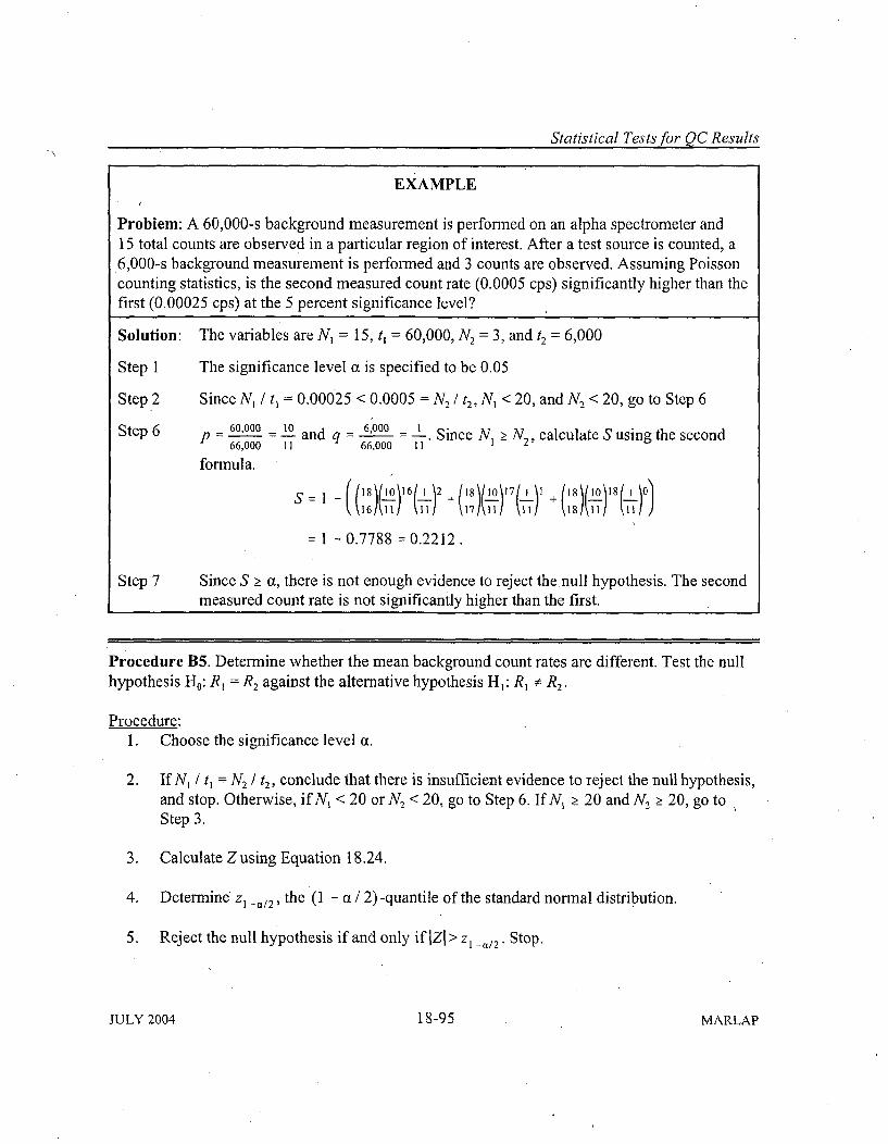
Statistical Tests for QC Results

EXAMPLE

Problem: A 60,000-s background measurement is perfonned on an alpha spectrometer and15 total counts are observed in a particular region of interest. After a test source is counted, a6,000-s background measurement is performed and 3 counts are observed. Assuming Poissoncounting statistics, is the second measured count rate (0.0005 cps) significantly higher than thefirst (0.00025 cps) at the 5 percent significance level?

Solution: The variables are N, = 15, t, = 60,000, N2 = 3, and t2 =6,000

Step I The significance level a is specified to be 0.05

Step 2 Since N, / t, = 0.00025 < 0.0005 =N 2 / t2, N, < 20, and N2 < 20, go to Step 6

Step 6 p 60in L and q - 6000 = I Since N > N2, calculate S using the second66,000 11 66,000 11

formula.

(( 1 8 ,( 1 6 (7 i\2 + (1 s1 ) f10 \1 7 ( i\ 1 11 \ 10 \ 8 (1 0"

S= 1 - ( (:') _\)I \11 + (1/i1 111 + ýT Is I ii!1)0

= 1 - 0.7788 = 0.2212.

Step 7 Since S Ž a, there is not enough evidence to reject the null hypothesis. The secondmeasured count rate is not significantly higher than the first.

Procedure B5. Determine whether the mean background count rates are different. Test the nullhypothesis H0: R, = R2 against the alternative hypothesis HI: R, t R2 .

Procedure:1. Choose the significance level (x.

2. If N, / t, = N2 / t 2, conclude that there is insufficient evidence to reject the null hypothesis,and stop. Otherwise, if N, < 20 or N2 < 20, go to Step 6. If N, Ž 20 and N, Ž 20, go toStep 3.

3. Calculate Z using Equation 18.24.

4. Determine zI -a/2, the (1 - a / 2)-quantile of the standard normal distribution.

5. Reject the null hypothesis if and only if IZI> zI -a/2. Stop.

JULY 2004 18-95 MARLAP

Statistical Tests for QC Results

6. If N1 / tj < N 2 / t2 , use Procedure B4 with significance level a / 2 to determine whetherR1 < R 2. IfN1 / tj > N2 / t2, use Procedure B4 with significance level a / 2 and with theobservations reversed to determine whether R2 < R1.

18B.4 Negative Activities'

When the measured count rate for a test source is less than that of the corresponding instrumentbackground, giving a negative value for the source activity, Procedure B4 may be used to deter-mine whether the difference between the two count rates is significantly more than should beexpected on the basis of the Poisson model and the assumption that the source is a'blank. (Let N,and tj be the source count and counting time and let N2 and t2 be the background count and count-ing time.). If a significant difference is found, it may indicate that the background measurementwas biased, the true background is variable or non-Poisson, or the instrument is unstable. Asbackground counts approach zero, the assumption of Poisson statistics begins to fail. This mean-centered approach may lead the analyst to an inappropriate conclusion. In these cases, anexamination of a larger population of blanks is more appropriate.

18B.5 References

Currie, Lloyd A. 1972. "The Limit of Precision in Nuclear and Analytical Chemistry." NuclearInstruments and Methods. 100(3), pp. 387-395.

U.S. Environmental Protection Agency (EPA). 2000. Guidance for Data Quality Assessment.Practical Methods for Data Analysis (G-9), QAOO Version. EPA/600/R-96/084, Washington,DC. Available at www.epa.gov/quality/qadocs.html.

Evans, Robley D. 1955. The Atomic Nucleus. McGraw-Hill, New York, NY.

Goldin, Abraham S. 1984. "Evaluation of Internal Control Measurements in Radioassay." HealthPhysics 47(3), pp. 361-374.

Knoll, Glenn F. 1989. Radiation Detection and Measurement, 2nd ed. John Wiley and Sons, NewYork, NY.

National Bureau of Standards (NBS). 1963. Experimental Statistics. NBS Handbook 91,Gaithersburg, MD.

MARLAP 18-96 JULY 2004