Market Entry and Structure Under Uncertain and Disparate

Market Expectations

or

Fools Rush In

Scott Carr¤

November 10, 2000

Abstract

An emerging market or market segment provides ¯rms both the opportunity to enter early

and capture market share and also the risk that the market will turn out to be less fruitful

than expected. We formulate and analyze a game-theoretic model in which multiple ¯rms with

uncertain and/or disparate beliefs about the eventual market size decide whether to enter such

a market. For increasingly general models, we show that the structure (i.e. the number and

identity of participating ¯rms) and pro¯tability of equilibrium oligopolies can be determined by

a classi¯cation scheme based on the ¯rms' beliefs about the viable level of market concentration.

This scheme is adapted to random forecasts (i.e. forecasts expressed as probability distributions)

as well as point forecasts. This study was motivated by managerial issues encountered by a client

¯rm engaged in semiconductor design.

¤The Anderson Graduate School of Management at UCLA, Los Angeles, CA, 90095-1481

1 Introduction

A new or emerging market or market segment provides both the opportunity to enter early and

capture market share and also the risk that the market will turn out to be less fruitful than

expected. This leads to a basic question of when/whether it is in a ¯rm's best interest to invest in

the development of products or facilities to serve a new market. The nature of a new market makes

this an inherently di±cult decision in that a ¯rm may need to commit its resources with limited

information about future demand, and the issue is further complicated by the likelihood that other

¯rms will also have the capability and the interest in entering this market. Furthermore, these

other ¯rms may have di®erent beliefs as to the eventual size of the market perhaps as a result of

di®erent information, past experiences, or forecasting techniques. How does the presence of these

competitor ¯rms and their di®ering opinions of future market size change the ¯rm's investment

decision? How do these di®erent opinions in°uence the market's structure (i.e. the number and

identity of participating ¯rms) and its pro¯tability? These are the questions addressed in this

paper.

This study was motivated by our work with a client ¯rm that designs, develops, and markets

semiconductor chipsets used in various types of digital communication. In this and other segments

of the semiconductor industry, an important managerial question is when to take an existing chipset

and adapt it to a new type of application. Such adaptation requires investing a substantial sum in

the design and development of an \Application Speci¯c Integrated Circuit," or \ASIC" in industry

parlance. For example, a chip originally designed for use in digital wireless telephones might be

adapted for use in digital wireless headsets; this is a new and potentially pro¯table application that

requires smaller size, lower power consumption, and reduced transmission energy.

Once an ASIC is developed, the ¯rm markets it to designers and assemblers of the communications

products; thus, the decision to invest in ASIC development occurs well in advance of complete

demand information. Indeed, the decision occurs in advance of even the design of the products

from which the ASIC demand will eventually derive. Consequently, the ¯rm must make this

investment decision with very limited information about the eventual demand for its chips, and

this is additionally confounded by the fact that other ¯rms are likely to be coincidentally developing

ASICs for the same market.

1

A key feature of this situation is that the ASIC development cost is an exogenous sunk cost in the

terminology of Sutton [1996] and others, and there is a substantial literature (see Sutton [1996], Hay

and Morris [1991], and the references therein) on the manner in which sunk costs are a determinant

of industry concentration. A basic result in that literature is that large exogenous sunk costs act

as a barrier to entry that induces market concentration (i.e. a small number of producers). This

paper extends that literature in that it introduces the idea that the ¯rms' forecasts or beliefs of

market conditions may be an additional determinate of industry concentration. If our models are

reduced to cases in which all ¯rms are able to accurately predict the market conditions, the models

would reduce to those already in the literature (again see Sutton, p. 27-45).

The sunk costs in our client's setting is a product development cost, but the analysis herein is

also applicable to other forms of sunk costs. For example, an investment in production facilities

and equipment is a sunk cost that is of much interest to the Operations-Management/Industrial-

Engineering community. Most models in that literature, such as the \newsvendor model" and

its many extensions (see Nahmias [1993] and references therein, Carr and Lovejoy [2000], Cachon

[1997]) consider the perspective of a single ¯rm in isolation. That is, the models do not recognize

that multiple ¯rms may be in competition and that the interaction between these ¯rms may have

important consequences to any individual ¯rm (e.g. an important input into a ¯rm's decision of

whether to build capacity to serve a new market is a prediction of the number of competitors who

will also enter that market). Recognizing that single ¯rm models do not capture the important

element of inter-¯rm competition, there is recent trend towards applying game theory to OM/IE

problems in competitive settings; for instance, Carr et. al. [2000] analyzes the interplay between

production variability and pro¯ts, van Mieghem and Dada [1999] considers the value of postpone-

ment strategies, and Cachon and Lariviere [1999] evaluate various inventory allocation schemes.

This paper is that vein in that it applies game theory modelling techniques and results (see Fried-

man [1990]) to the issues of uncertainty, forecasting, and capacity investment that are common in

the OM/IE literature.

Conversely, there are also papers that incorporate uncertainty and forecasting into economic models

of industry concentration and market entry. For example, Maskin [1999] considers how uncertainty

about demand and costs impacts an incumbent's decision of how much production capacity to

install and the ability of this capacity to deter others from entering the industry, Dixit [1989]

models an individual ¯rm's entry and exit decisions when price follows a random walk, and De

2

Wolf and Smeers [1997] analyze a Stackelberg game in which the leader makes its production

decision under demand uncertainty and the followers make their production decisions after the

uncertainty is resolved. In our paper, entry decisions are made by multiple ¯rms while demand is

uncertain, and production decisions are made after the uncertainty is resolved.

In the next section we specify a model with two decision stages in which multiple ¯rms ¯rst

simultaneously decide whether to invest the sunk cost (e.g. the ASIC development cost) and enter

a new market based on forecasted market conditions. Sometime after committing themselves to

entry, the ¯rms learn the actual market conditions, and the ¯rms then use this new information to

determine their production quantities. Finally, these production quantities together with the actual

market conditions determine the selling price and ¯rms' pro¯ts. Sections 3 through 5 investigate

the above-described issues under increasingly general conditions about the nature of the ¯rms'

forecasts. Section 6 relaxes the assumption that entry decisions are made simultaneously by all

the ¯rms. Section 7 provides very general model under which all of our primary results hold; this

model includes di®erent modes of competition, Bertrand or price-setting competition for instance.

Below are some of the insights derived from these models:

1. The equilibrium market structure (i.e. the level of industry concentration and the identity of

the market entrants) is determined by the beliefs or forecasts that ¯rms have of the actual

conditions that will be experienced post-entry. For example, there may be a large number of

potential entrants, but these ¯rms may have low expectations for the market; this will result

in a small number of entrants.

2. The market structure also depends upon the manner in which beliefs are \distributed" among

potential participants. That is, a case in which ¯rms have very similar forecasts of market

conditions often results in a very di®erent structure than a case in which the ¯rms' forecasts

are very dispersed or heterogeneous.

3. The market structure can be determined by a simple classi¯cation scheme based on ¯rms'

pre-entry beliefs, and this scheme is very robust to changes in the underlying assumptions.

4. The pro¯ts earned by the market participants are determined by both the actual market con-

ditions and also by the market structure. Since the potential participants' forecasts determine

market structure, they are an important albeit indirect determinant of market pro¯tability.

3

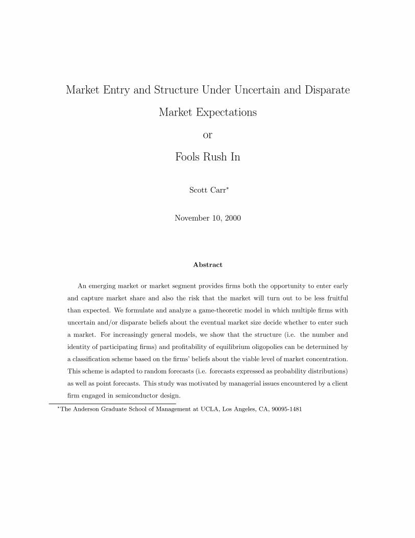
N Firms forecastmarket

conditions

Stage 1:Entry

Decision

Stage 2:QuantityDecision

Fixed costC

incurred

Firms learnmarket

conditions

Price isestablished,

andrevenues

are earned

Figure 1: Sequence of Events

5. Firms may represent their forecasts as probability distributions to recognize their uncertainty

about the market conditions. Increased variance in such a distribution makes it more likely

that the ¯rm will enter the market and less likely that the ¯rm will be pro¯table.

6. Firms who forecast a large market are more likely participants than ¯rms that forecast a

small market, but this is only partially true. To a limited extent, participating ¯rms may

forecast a smaller market than other non-participating ¯rms.

7. It is intuitively obvious and analytically true that the ¯rms most likely to enter a new market

are those who grossly overforecast the market's potential. If there are only a small number

of these ¯rms, then the overall market pro¯tability will not su®er. This situation changes if

there are a large number of these ¯rms. If a su±cient number of ¯rms share a su±ciently

rosy view of the market's potential, then so many ¯rms will rush into the market that it is

unpro¯table for all; hence this paper's subtitle.

2 Preliminaries

First, a brief statement of the model as illustrated by ¯gure 1. There are initially N ¯rms who

simultaneously choose whether to invest a ¯xed and sunk cost C to enter a new market; this cost

represents the ASIC development cost in our industrial setting. The ¯rms may also costlessly decide

not to enter. Importantly, the ¯rms decide whether to enter the market before they know the actual

market conditions, so they are unable to accurately predict the price that they will ultimately receive

for their goods and must base their entry decision on a forecast of market conditions. Once all ¯rms

have made an entry/no-entry decision, they receive more accurate market information and then

choose a quantity to produce. The actual price is ultimately determined by the quantity that the

entrants produce in aggregate. The model is thus a two-stage game; ¯rms make the entry decision

4

in the ¯rst stage and the production decision in the second stage, and they receive additional

market information between the stages. We employ the sub-game perfect Nash equilibrium for

this competitive model, and we restrict attention to pure strategies. The three following sections

describe models that di®er in the forecasting assumptions; the remainder of this section describes

modeling elements that are common to those models.

Market Conditions: We assume that the common post-production price p that is received by

the ¯rms is related to the aggregate quantity Q that is produced by all ¯rms through the linear

relation

p = a¡ bQ with a; b > 0 (1)

The intercept a represents the market's reservation price (the supremum price at which demand

is positive), and the slope b is the elasticity of price with respect to Q. An individual ¯rm i's

production decision is denoted qi, so Q :=Pi qi.

Stage 1, Market entry: All N potential entrants simultaneously decide whether to invest C and

enter the market. We assume, and this is assumption is central to our model, that the ¯rms do

not know the market's reservation price at the time of the entry decision. Rather, they calculate

their anticipated post-entry margins based on a forecasted reservation price; speci¯c forecasting

assumptions will be discussed in the sections that follow.

Each possible (but perhaps not equilibrium) set of entry decisions is represented by an \entry

vector." This is an N -vector in which the i-th element represents ¯rm i's entry/no-entry decision,

and we say that ¯rms are \members," \entrants," or \participants" if they have selected entry in

that vector. It may be that membership in an entry vector is undesirable to one or more ¯rms; we

say that these ¯rms are \willing to leave" the vector. This occurs when a member anticipates that

post-production revenues will be less than C. In other words, member ¯rms are willing to leave

if they believe that a non-entry decision, which guarantees zero pro¯ts, would be preferable to an

entry decision given that the second-stage oligopoly will consist of the other members of that entry

vector.

Similarly, it may be that non-members of an entry vector would prefer membership. In this case

we say that these non-members are \willing to enter" the entry vector, and this occurs when they

believe that an entry decision would be preferable to their current non-entry decision. Of course,

5

it must be that no ¯rms are willing to enter or to leave an equilibrium entry vector.

Our intention is not to analyze the manner in which di®erent forecasting techniques lead to di®erent

forecasts, but rather to understand how the error and uncertainty that is inherent in any forecasting

method a®ects the structure and pro¯tability of a new market. We thus assume that each ¯rm's

entry decision is made on the basis of the forecasted reservation price, the required investment,

the entry decisions of its competitor ¯rms, and the anticipated post-entry production decisions of

those competitors, and we exclude the possibility that a ¯rm may, indeed perhaps should, actually

change or update its own forecast upon receiving information about which other ¯rms are electing

to enter the market. This is a case of bounded rationality as discussed by Conlisk [1996].

Stage 2, Production: At the beginning of stage 2, the ¯rms learn the actual reservation price.

Each ¯rm then selects a production quantity, and the market price p is determined by (1). A ¯rm

i who has chosen to enter the market thus receives revenue of qi ¢ p for a net pro¯t of qi ¢ p ¡ C.This implicitly assumes the variable production costs are zero; relaxing this is a straightforward

step, which we do not take, that adds notational complexity without providing additional insight.

The production decision of non-members is simply handled by forcing their production quantities

to be zero.

Before introducing speci¯c forecasting assumptions, it may be noted that this model is a form of the

\market-entry games" described by Selten and G::uth [1982] and Gary-Bobo [1990]. The primary

di®erence between those games and our models is that we introduce forecasting and focus upon

its consequences. Nonetheless, it is possible to prove equilibrium existence in our models from

Gary-Bobo's primary result.

3 Entry and Structure with Three Forecasting Classes

The model of this section is the simplest and illustrates several results that are shared by the more

complicated models that follow. Here we assume that each ¯rm falls into one of three forecasting

classes, high, accurate, or low (abbreviated by subscripted \hi", \ac", \lo"), and that the number

of ¯rms in each class is some large integer. Also, we assume here and throughout that ¯rms only

desire membership in a market when their anticipated pro¯ts are strictly positive; this assumption

eliminates some trivial cases and is otherwise benign.

6

In stage-1, high-forecasters anticipate a reservation price fhi > a, accurate forecasters correctly

forecast a reservation price fac = a, and low-forecasters anticipate a reservation price flo < a.

Again, the actual reservation price a is learned at the beginning of stage 2.

Equilibrium: As is typical, subgame-perfect equilibrium conditions are identi¯ed by working in a

backward direction, so we begin by assuming a known entry vector from stage-1, and we let n be

the number of members in that vector.

The subgame-perfect equilibrium requires that in the terminal stage-2, given an entry vector, the

member ¯rms in that vector reach a standard Nash equilibrium in production quantities. Also, the

only di®erence between ¯rms in this game is their forecasts, but these are of no importance during

stage two because the forecasts have been replaced by accurate market information. Thus, all ¯rms

are essentially identical when they select a production quantity. It follows that the equilibrium

production decisions will be the same as for a Cournot (i.e. quantity-setting) oligopoly of size n in

which all oligopolists have accurate market information.

Speci¯cally, suppose that each member ¯rm i selects a production quantity qi. Then the second-

stage equilibrium condition is that i's production quantity is its revenue maximizing quantity given

that its competitors will collectively produce quantityPj 6=i qj . It is straightforward to show (see

appendix for derivations) using ¯rst order optimality conditions that the unique solution to this

condition is for every member ¯rm to produce quantity

a

b (1 + n): (2)

Each member ¯rm will then earn pro¯ts of

a2

b (1 + n)2¡ C (3)

Now moving to stage-1, ¯rms here decide whether to enter the market, so we seek a subgame-perfect

equilibrium entry vector. This is an entry vector that no ¯rms are willing to enter or leave given

that they anticipate that post-entry they will receive pro¯ts as in (3). But, ¯rms' entry decisions

are based not on actual but rather on forecasted reservation prices, so a ¯rm with forecast f (i.e.

a ¯rm that anticipates a reservation price of f) believes that membership in an entry vector that

has n total members will yield pro¯ts

f2

b (1 + n)2¡ C

7

which will be positive when

n <fpbC

¡ 1

Or, since the number of entrants must be an integer, the ¯rm anticipates positive (negative) pro¯ts

from membership in an entry vector with ¹fpbC

¡ 1º

(4)

or fewer (more) ¯rms1. Put another way, (4) is the maximum number of entrants that the ¯rm

believes that the market can pro¯tably support. The ¯rm is thus willing to enter any vector with

strictly fewer than this number of members but is unwilling to enter any vector with this number

or more members.

Let K denote the equilibrium number of ¯rms that, unbeknownst to the stage-1 competitors, the

market can actually support. This is calculated by replacing the forecast f in (4) by the actual

reservation price a to get

K =

¹apbC

¡ 1º

(5)

Next de¯ne another value fK as the in¯num forecast such that a ¯rm with this forecast would

anticipate that the market can support K ¯rms. It can be derived (see appendix) that

fK =pbC

¹apbC

º(6)

We can now characterize the equilibrium market structure for this ¯rst set of forecasting assump-

tions.

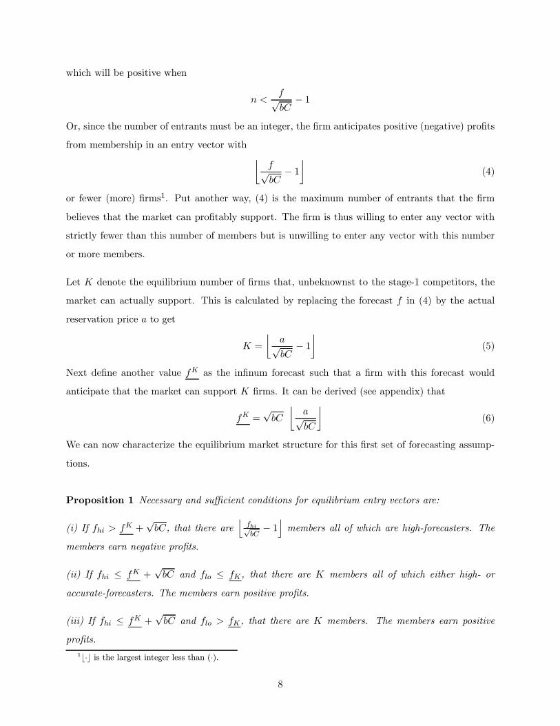
Proposition 1 Necessary and su±cient conditions for equilibrium entry vectors are:

(i) If fhi > fK +pbC, that there are

jfhipbC¡ 1

kmembers all of which are high-forecasters. The

members earn negative pro¯ts.

(ii) If fhi · fK +pbC and flo · fK, that there are K members all of which either high- or

accurate-forecasters. The members earn positive pro¯ts.

(iii) If fhi · fK +pbC and flo > fK , that there are K members. The members earn positive

pro¯ts.

1b¢c is the largest integer less than (¢).

8

As stated in the proposition, there are three possible scenarios. In the ¯rst scenario ((i) in the

proposition) the high forecasters are very overoptimistic about the size of the market. In fact,

they are so overoptimistic that they oversaturate the market and lose money. In other words, too

many fools rush into the market. Additionally, the accurate- and low-forecasters anticipate this

happening and wisely stay out. In scenario (ii), the accurate- and high-forecasters have such similar

expectations about the market that they are indistinguishable with regard to their entry decisions.

The low-forecasters, however, are much less optimistic than the other groups, so they will unwisely

decline entry. Equilibrium vectors thus consist of any K ¯rms from the two higher forecasting

classes. In (iii), the groups all have such similar forecasts that they make their entry decisions as

if they have exactly the same forecast, the accurate one.

Thus we see that two factors together determine whether a ¯rm is a member of an equilibrium

vector. The ¯rst and most obvious is the ¯rm's own expectation of market size; ¯rms with high

expectations are more likely to enter the market. The second factor is the disparity between ¯rms'

forecasts. For example, we see in the proposition that whether an accurate-forecasting ¯rm is a

market entrant is determined by the degree to which its more rosy-eyed competitors overforecast.

The proposition also implies several other results about the equilibrium structure:

1. low- and accurate-forecasters will never earn negative pro¯ts. They may, however, exclude

themselves from the market if the high-forecasters are su±ciently overoptimistic.

2. Member ¯rms, including the high-forecasters, make positive pro¯ts if and only if there is an

equilibrium vector with an accurate-forecaster member.

3. Pro¯ts earned by each member ¯rm weakly decrease with fhi. This is because the number of

equilibrium members increases with fhi, and the members' pro¯ts decrease with the number

of members. Also, the aggregate pro¯ts of all member ¯rms weakly decreases with fhi; this

follows from the additional fact that aggregate oligopoly pro¯ts are maximized when there is

only a single ¯rm (i.e. the oligopoly is actually a monopoly) and are thereafter decreasing in

the number of ¯rms.

4. There are always at least K ¯rms in any equilibrium. This occurs because we have assumed

a large number of accurate- and high-forecasters. This result does not hold if the aggregate

number of ¯rms in these classes is less than K.

9

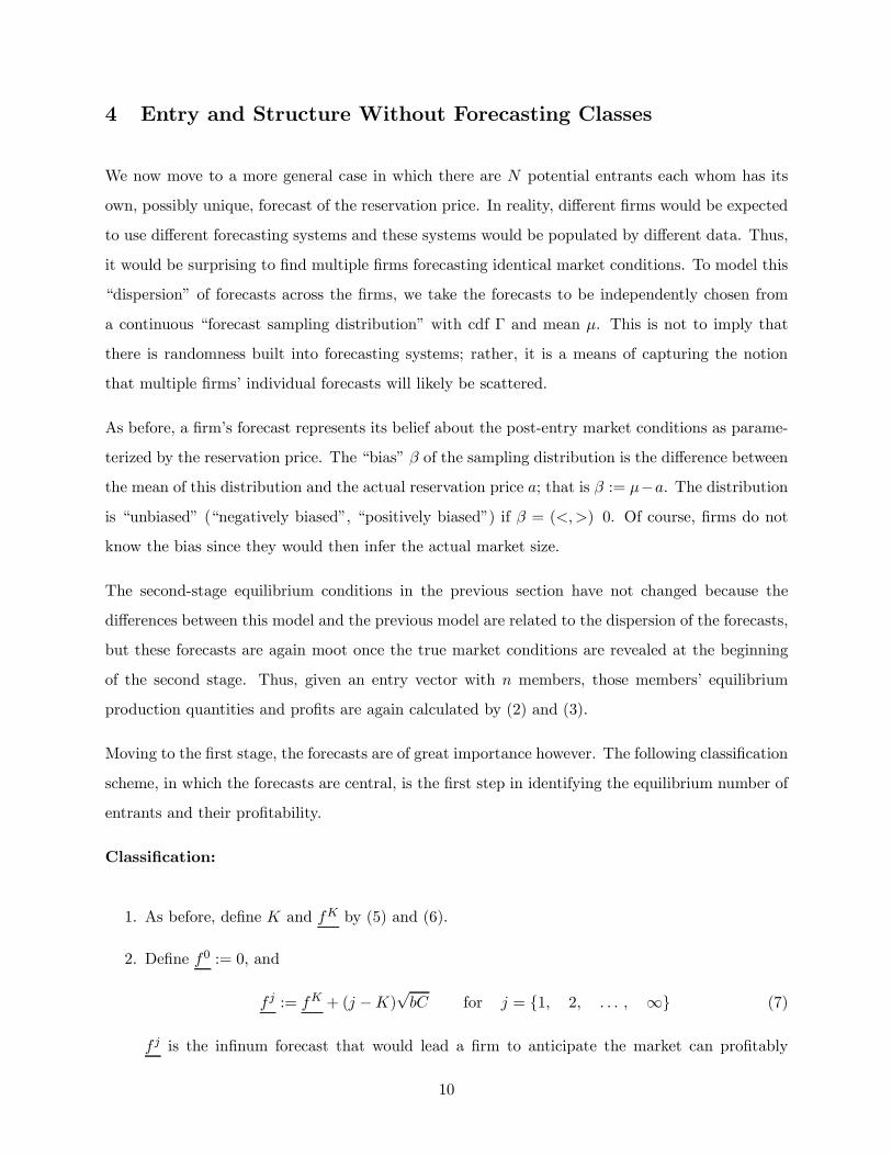
4 Entry and Structure Without Forecasting Classes

We now move to a more general case in which there are N potential entrants each whom has its

own, possibly unique, forecast of the reservation price. In reality, di®erent ¯rms would be expected

to use di®erent forecasting systems and these systems would be populated by di®erent data. Thus,

it would be surprising to ¯nd multiple ¯rms forecasting identical market conditions. To model this

\dispersion" of forecasts across the ¯rms, we take the forecasts to be independently chosen from

a continuous \forecast sampling distribution" with cdf ¡ and mean ¹. This is not to imply that

there is randomness built into forecasting systems; rather, it is a means of capturing the notion

that multiple ¯rms' individual forecasts will likely be scattered.

As before, a ¯rm's forecast represents its belief about the post-entry market conditions as parame-

terized by the reservation price. The \bias" ¯ of the sampling distribution is the di®erence between

the mean of this distribution and the actual reservation price a; that is ¯ := ¹¡a. The distributionis \unbiased" (\negatively biased", \positively biased") if ¯ = (<;>) 0. Of course, ¯rms do not

know the bias since they would then infer the actual market size.

The second-stage equilibrium conditions in the previous section have not changed because the

di®erences between this model and the previous model are related to the dispersion of the forecasts,

but these forecasts are again moot once the true market conditions are revealed at the beginning

of the second stage. Thus, given an entry vector with n members, those members' equilibrium

production quantities and pro¯ts are again calculated by (2) and (3).

Moving to the ¯rst stage, the forecasts are of great importance however. The following classi¯cation

scheme, in which the forecasts are central, is the ¯rst step in identifying the equilibrium number of

entrants and their pro¯tability.

Classi¯cation:

1. As before, de¯ne K and fK by (5) and (6).

2. De¯ne f0 := 0, and

f j := fK + (j ¡K)pbC for j = f1; 2; : : : ; 1g (7)

f j is the in¯num forecast that would lead a ¯rm to anticipate the market can pro¯tably

10

Forecasts

6f 7f 8f 9f

a10f 11f

if

5 6 7 8 9 10Class

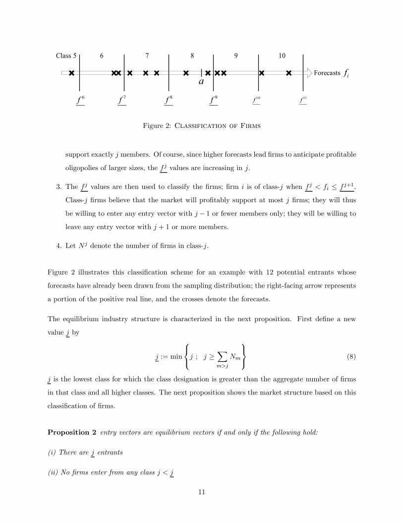
Figure 2: Classification of Firms

support exactly j members. Of course, since higher forecasts lead ¯rms to anticipate pro¯table

oligopolies of larger sizes, the f j values are increasing in j.

3. The f j values are then used to classify the ¯rms; ¯rm i is of class-j when f j < fi · f j+1.

Class-j ¯rms believe that the market will pro¯tably support at most j ¯rms; they will thus

be willing to enter any entry vector with j ¡ 1 or fewer members only; they will be willing toleave any entry vector with j + 1 or more members.

4. Let N j denote the number of ¯rms in class-j.

Figure 2 illustrates this classi¯cation scheme for an example with 12 potential entrants whose

forecasts have already been drawn from the sampling distribution; the right-facing arrow represents

a portion of the positive real line, and the crosses denote the forecasts.

The equilibrium industry structure is characterized in the next proposition. First de¯ne a new

value j by

j := min

8<:j ; j ¸ Xm>j

Nm

9=; (8)

j is the lowest class for which the class designation is greater than the aggregate number of ¯rms

in that class and all higher classes. The next proposition shows the market structure based on this

classi¯cation of ¯rms.

Proposition 2 entry vectors are equilibrium vectors if and only if the following hold:

(i) There are j entrants

(ii) No ¯rms enter from any class j < j

11

(iii) Every ¯rm in all classes j > j enters

(iv) Exactly j ¡Pm¸j+1Nm ¯rms from class j enter

(v) The entering ¯rms in all entry equilibria will earn positive pro¯ts i® j · K, and this occurs ifthere are more than K ¯rms in classes higher than j .

(iv) There are µN j

j ¡Pm¸j+1Nm

¶equilibrium entry vectors.

We think of ¯rms in class-j as good forecasters because they have forecasts that may not be perfect

but are su±ciently accurate to induce the ¯rm to behave in exactly the same manner as a ¯rm that

does have a perfect forecast. We think of ¯rms in classes lower than j as conservative forecasters.

From the proposition, and analogous to results from the previous section, good and conservative

forecasters can never lose money because they will exclude themselves from entry if the market is

not su±ciently concentrated.

We think of ¯rms in classes higher than j as overoptimistic. From (i) and (v), the pro¯tability of

these ¯rms depends on the number of other overoptimistic ¯rms and on the manner in which their

forecasts are scattered. If j is greater than K, then an overoptimistic ¯rm will be unpro¯table if it

enters, but it will not enter if there are su±ciently many ¯rms that are even more optimistic (and

therefore in higher classes).

It is also true that equilibrium pro¯ts are weakly decreasing in any ¯rm's forecast. This is because:

(1) an increase in one ¯rm's forecast may push the ¯rm into a higher class, (2) this may increase

the equilibrium number of ¯rms, and (3) this would reduce the pro¯tability of every entrant.

Before moving on, it is interesting to note that a will always fall between fK and fK+1: Thus, a

¯rm that accurately forecasts demand to be exactly a will be in class-K; it follows from proposition

2 that if a perfect-forecaster such as this is a member of an equilibrium vector, then all ¯rms in

any equilibrium vector will earn positive pro¯ts.

Another interesting question is: what is the a priori probability that ¯rms in an equilibrium

oligopoly will be pro¯table? An entry vector will be pro¯table if and only if it has K or fewer

12

members. This will be the case in equilibrium entry vectors i® K or fewer ¯rms are in classes

(K + 1) through 1; or, equivalently, that K or fewer ¯rms receive forecasts that are > fK +pbC.

This probability, derived from the binomial distribution, is given in the following proposition the

proof of which is in the appendix.

Proposition 3 Prior to assigning forecasts to ¯rms, the probability that any ¯rms will be pro¯table

at equilibrium is:

1 if N · K

PKj=0

¡Nj

¢ h1¡ ¡

³fK +

pbC´ij h

¡³fK +

pbC´iN¡j

if N > K

When N > K, this probability is decreasing in the bias of the sampling distribution ¯ and the

number of ¯rms N ; it is increasing in the market reservation price a.

Intuitively, positive equilibrium pro¯ts become less likely as ¯ or N increases because this leads to

larger equilibrium oligopolies and more intense post-entry competition. For rising ¯, equilibrium

oligopolies get larger because ¯rms become more likely to overforecast the market size. For an

increased N , it is because the expected number of ¯rms with optimistic forecasts increases. In

contrast, a rising reservation price a does not change the size of equilibrium oligopolies; this is

because entry decisions are based not on a but instead on the ¯rms' forecasts of a. What does

change is that pro¯ts increase with a for any entry vector which leads to a higher probability of

pro¯table equilibria.

Now consider the special case in which the forecast sampling distribution is a normal distribution

with mean ¹ and standard deviation ¾. The probability that ¯rms will be pro¯table at equilibrium

is now

KXj=0

µN

j

¶©j

á fK +

pbC ¡ ¹¾

!©N¡j

ÃfK +

pbC ¡ ¹¾

!(9)

where © is the standard Normal cdf. In this case, we can make the additional claim that the prob-

ability that ¯rms will be pro¯table at equilibrium decreases with the sampling standard deviation

¾ if and only if the sampling distribution bias is < fK +pbC ¡ a. The proof of this claim follows

from the arguments in the proof of proposition 3 (see appendix), the de¯nition of ¯, and the fact

13

that the probability of a success, as de¯ned in the appendix, increases with ¾ if and only if the

numerators in the above expression are positive.

Example 1 illustrates the model and results of this section.

Example 1: A new market with N = 13 potential entrants has a = 250 and b = 1. The potential

entrants' forecasts of the reservation price a are sampled from a normal distribution with mean

¹ = 275 and standard deviation ¾ = 30, and the investment required to enter this market is

C = 650. By (5), this market is able to pro¯tably support K = 8 ¯rms. Applying (9), prior to the

sampling of the forecasts there is aP8j=0

¡13j

¢©j (¡:667) ©13¡j (:667) = 21:2 percent probability

that the members of any equilibrium will be pro¯table. To a large extent, this low probability is due

to a positive bias of the sampling distribution of ¯ = ¹¡ a = 25.

fK = 229:5 from (6), so the bias is greater than fK +pbC ¡ a = 4:95 which implies that this prob-

ability will increase with any increase in the sampling distribution's standard deviation ¾. Indeed,

this probability is quite sensitive to changes in ¾; if ¾ is reduced to 20, the probability is only 4:2%;

if ¾ is increased to 40, the probability increases to 37:1%.

Table 1 gives the critical values of the classi¯cation scheme. Table 2 gives forecasts drawn from the

sampling distribution for each of the 13 ¯rms; the table also indicates each ¯rm's classi¯cation.

14

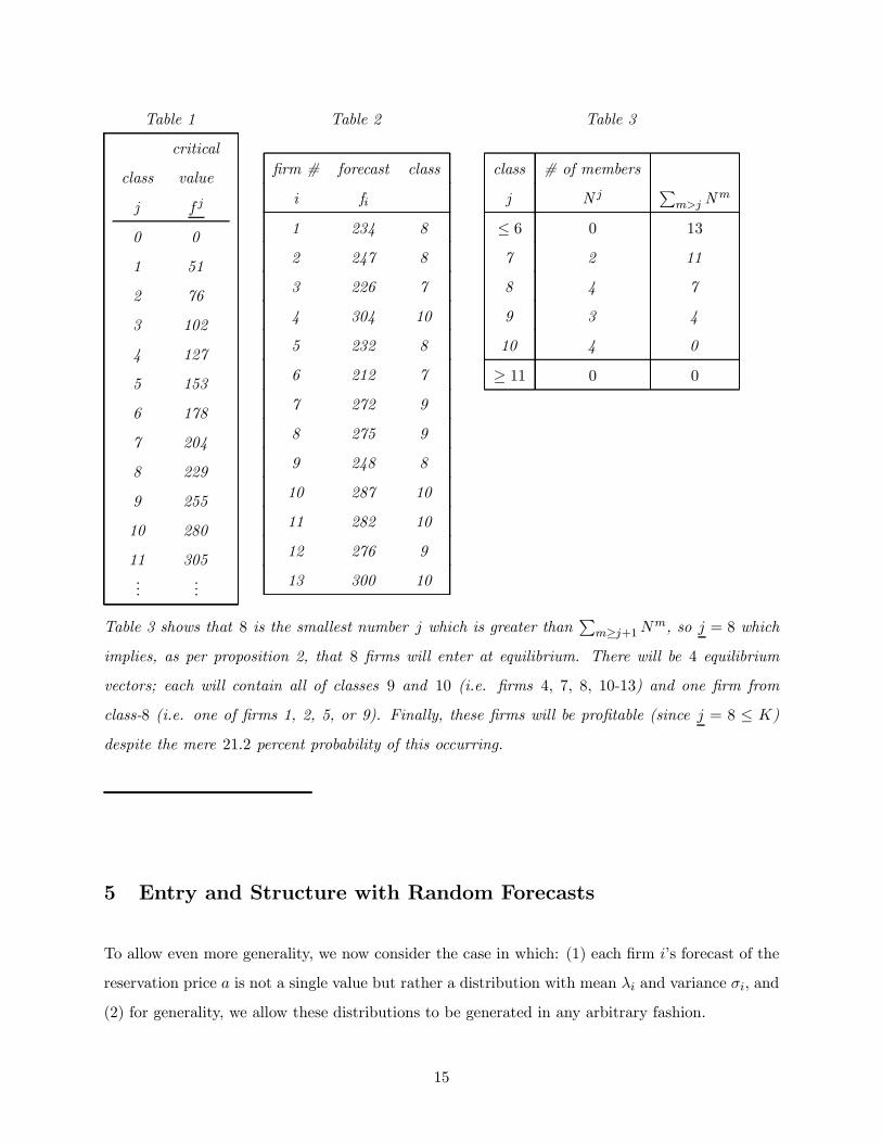
Table 1 Table 2 Table 3

critical

class value

j f j

0 0

1 51

2 76

3 102

4 127

5 153

6 178

7 204

8 229

9 255

10 280

11 305...

...

¯rm # forecast class

i fi

1 234 8

2 247 8

3 226 7

4 304 10

5 232 8

6 212 7

7 272 9

8 275 9

9 248 8

10 287 10

11 282 10

12 276 9

13 300 10

class # of members

j N jPm>j N

m

· 6 0 13

7 2 11

8 4 7

9 3 4

10 4 0

¸ 11 0 0

Table 3 shows that 8 is the smallest number j which is greater thanPm¸j+1N

m, so j = 8 which

implies, as per proposition 2, that 8 ¯rms will enter at equilibrium. There will be 4 equilibrium

vectors; each will contain all of classes 9 and 10 (i.e. ¯rms 4, 7, 8, 10-13) and one ¯rm from

class-8 (i.e. one of ¯rms 1, 2, 5, or 9). Finally, these ¯rms will be pro¯table (since j = 8 · K)despite the mere 21:2 percent probability of this occurring.

5 Entry and Structure with Random Forecasts

To allow even more generality, we now consider the case in which: (1) each ¯rm i's forecast of the

reservation price a is not a single value but rather a distribution with mean ¸i and variance ¾i; and

(2) for generality, we allow these distributions to be generated in any arbitrary fashion.

15

The second stage equilibrium conditions remain unchanged from the previous sections, again be-

cause the ¯rms are only di®erentiated by their forecasts which are rendered moot by knowledge

of the actual reservation price. That is, given an entry vector with n members, the equilibrium

second-stage quantities and revenues are still given by (2) and (3). The ¯rst-stage entry equilibrium

conditions conceptually remain unchanged in that equilibrium vectors are those entry vectors that

no ¯rms are willing to enter or leave. These decisions are now made on the basis of whether expected

second-stage revenues will exceed the ¯xed cost C.

Given a ¯rst-stage entry vector with n members, a member ¯rm i's expected second-stage revenues

are Eh

a2

b(1+n)2

iwhich equals

E[a2]b(1+n)2

with the expected value taken over i's forecast distribu-

tion. As is true of all probability distributions, ¾2i = E£a2¤¡ ¸2i , so we substitute ¸2i + ¾2i for the

numerator to get expected revenues of

¸2i + ¾2i

b (1 + n)2(10)

The fact that this increases with forecast mean ¸i is entirely intuitive; a larger market, param-

eterized by a larger a, equals stronger demand and higher pro¯ts, so a higher expectation of a

translates into a higher expectation of pro¯ts. The fact that (10) increases with forecast std ¾i is

less intuitive; in follows from the convexity of pro¯ts in a (see (3)) and Jensen's inequality.

This means that ¯rm i believes, based on its forecast distribution, that member ¯rms in an entry

vector will be pro¯table (in expected value) if

¸2i + ¾2i

b (1 + n)2¡ C > 0

or, equivalently, if the number of members n is less than or equal to$r¸2i + ¾

2i

bC¡ 1

%This now becomes the basis for a classi¯cation scheme as in the previous section. In fact we can use

the previous scheme with a straightforward generalization to account for the forecast randomness.

We now place a ¯rm in class-j when f j ·q¸2i + ¾

2i < f

j+1. Under this classi¯cation scheme:

1. The classes can be interpreted as before; class-j ¯rms believe that the market can pro¯tably

support j or fewer ¯rms.

2. Proposition 2 holds unchanged.

16

1 32 4 5 6 7 8 9 10a

Class

x

y

Forecast mean λ!

Fore

cast

std.

σ!

z

Figure 3: Classification with Disbursed Random Forecasts

3. Members' expected pro¯ts increase in both the mean and variance of their forecast distribu-

tions in any entry vector. This can be easily seen from (10) and includes all equilibrium entry

vectors.

4. But, members' actual equilibrium pro¯ts weakly decrease in both the mean and variance of

their forecast distributions. This happens because the increased expected pro¯ts (see previous

point) may result in additional members at equilibrium and because the actual pro¯ts of the

equilibrium members is decreasing in the number of members but unchanging in any ¯rm's

forecast (with the number of entrants ¯xed).

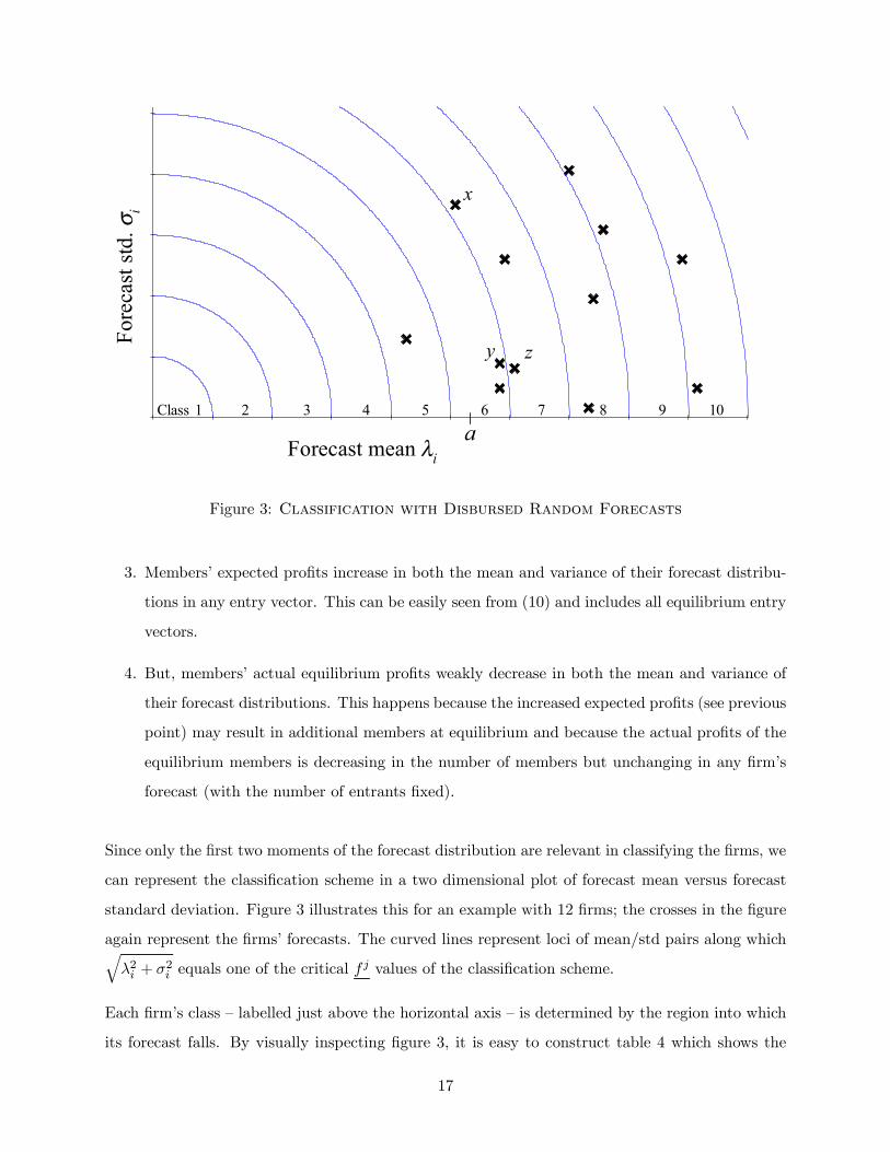
Since only the ¯rst two moments of the forecast distribution are relevant in classifying the ¯rms, we

can represent the classi¯cation scheme in a two dimensional plot of forecast mean versus forecast

standard deviation. Figure 3 illustrates this for an example with 12 ¯rms; the crosses in the ¯gure

again represent the ¯rms' forecasts. The curved lines represent loci of mean/std pairs along whichq¸2i + ¾

2i equals one of the critical f

j values of the classi¯cation scheme.

Each ¯rm's class { labelled just above the horizontal axis { is determined by the region into which

its forecast falls. By visually inspecting ¯gure 3, it is easy to construct table 4 which shows the

17

number of ¯rms in each class. By (8) and proposition 2, j = 7 is the equilibrium number of

members. As is also shown in the ¯gure, the actual reservation price a falls into the region of

class-6 (i.e. K = 6). Thus, since j > K, the equilibrium will not be pro¯table.

Table 4

class # of members

j N jPm>j N

m

1 ¡ 4 0 12

5 1 11

6 2 9

7 3 6

8 2 4

9 2 2

10 2 0

We also see in this example that while equilibria tend to be populated by ¯rms who anticipate

a large market size, there is not a monotonic relationship between a ¯rm's forecast mean and its

inclusion in an equilibrium. This is, we cannot say that if ¯rms x and y have forecast means ¸x

and ¸y with ¸x < ¸y then any equilibrium that includes x also includes y. There are two reasons

that x but not y might be a member of an equilibrium. First, it may be that x's forecast standard

deviation is su±ciently high that x is in a higher class than is y. This case is illustrated by the

labelled points in the ¯gure. Firm x is in class-7 and there are 7 member ¯rms at equilibrium, so

there exists an equilibrium with x as a member. Not so for y, that ¯rm is in class-6 and is thus

excluded from any equilibrium. It is easy to see that x's large forecast standard deviation dominates

the fact that its forecast mean is smaller than y's. The other possible scenario is illustrated by

the points x and z. Both are in class-j, and each equilibrium vector has one ¯rm from that class.

There is therefore an equilibrium vector with x but not z as a member even though ¸x < ¸z. Of

course this also means that there is an equilibrium vector that includes z but not x.

18

6 A Sequential Equilibrium Selection Process

We have thus far simply presumed that all ¯rms declare their entry decision simultaneously, but

this might be a substantial departure from the manner in which real ¯rms approach market entry

decisions. It is quite possible that the entry decisions of real ¯rms will be: (1) sequential { ¯rms'

decision-making processes might naturally be staggered in time; (2) phased { ¯rms may announce

an intention to enter prior to making an irreversible entry commitment; and/or (3) based on simpler

criteria and/or less information than is presumed by the subgame perfect Nash equilibrium. We

were thus interested in whether there is a process that includes these features and that terminates

in an equilibrium entry vector as characterized by proposition 2. Indeed, the process described

below is such a process. Additionally, this process typically terminates in a small number of steps

(actually, \rounds" as described below) at a unique equilibrium vector, and it terminates in a quite

natural fashion.

The process is initialized by specifying an arbitrary entry vector (e.g. a vector with no members)

and an arbitrary sequence of the potential entrants. The process then consists of a number of

rounds. In each round the ¯rms sequentially decide whether membership in the vector is desirable.

We presume that the ¯rms make this decision based on a very simple criterion: a class-j ¯rm will

select membership in a vector if the number of other competitors who are already members is less

than j and otherwise select non-membership. That is, the ¯rm selects membership if and only if

its membership will result in a total number of members that is · the number that ¯rm believes

can be pro¯tably supported.

The ¯rst round begins with the ¯rst ¯rm making a membership decision based on the initial entry

vector, and the vector is updated with that ¯rm's membership decision. The next ¯rm then chooses

membership/non-membership based on this updated vector, and the vector is again updated. The

process continues in this fashion with updating of the vector after each ¯rm. Each round ends after

the vector is updated with the N -th ¯rm's decision, and the next round begins with the ¯rst ¯rm

reacting to that vector. The process terminates when the vector remains constant throughout an

entire round.

It can be shown that this simple process terminates in a ¯nite number of rounds in a unique

equilibrium entry vector. The proof of this claim is omitted for brevity; the proof proceeds by

19

showing that, after the ¯rst round and prior to the terminal round, the entry vector seen by the

¯rst ¯rm is strictly monotonic under a form of lexicographic ordering. The set of possible entry

vectors is ¯nite, so termination in a ¯nite number of rounds is guaranteed. The fact that the

terminal vector is an equilibrium vector follows directly from the termination condition that the

entry vector remains constant through an entire round; this would not occur if any ¯rm has an

incentive to unilaterally deviate from their membership decision in the terminal vector.

7 A General Formulation and Price Competition

The basic results about market structure have thus far relied heavily on speci¯c assumptions about

the nature of the investment (scalar and independent of any other decision), demand (price is

linear in aggregate quantity), and mode of competition (quantity-setting). This section gives a

more general formulation to illustrate that the results are actually quite robust to changes in the

model. Under this much weaker set of assumptions the technique of mapping each ¯rm's forecast

into a belief about the largest number of ¯rms that can be pro¯tably supported, classifying the ¯rms

based on this belief, and using this classi¯cation to characterize the equilibrium market structure

remains valid. As an example, we show how the model may be adapted to a setting in which ¯rms

compete by setting prices rather than quantities.

Let A be the set of possible market conditions. Contained within A are both the actual market

condition (e.g. the market reservation price in the previous models) and also all possible forecasts

of this market condition. The set A, and of course the actual market condition and all forecasts,

may now be multi-dimensional Real vectors or could be taken from some more arbitrary set as in

the price-competition example that follows.

Decision stage 1: Initially with N potential entrants into the new market, each ¯rm i has a

forecast fi 2 A. In the ¯rst decision stage, each ¯rm then decides whether to enter the market

by selecting and entry decision ei from the set fenter; do not enterg. This gives an entry vector(e1; e2; ::: ; eN ) each element of which is one ¯rm's entry decision, and we let E be the set of all

possible entry vectors.

Decision stage 2: Next, the actual market condition a 2 A is revealed and each ¯rm selects a

second stage strategy. S denotes the set of strategies that are available to each ¯rm, and it includes

20

the element 0. Thus, each ¯rm i selects a strategy si 2 S to give a strategy vector (s1; s2; ::: ; sN);note however that any ¯rm that selected no entry in stage 1 is restricted to selecting 0 in the second

stage. De¯ne § as the N -dimensional S£S £ :::£S; this is the set of all possible strategy vectors.

Pro¯ts: Finally, pro¯ts are calculated by a pro¯t function ¼ : §£A£E ¡! <N . This is a vectorfunction, and its i-th element ¼i represents ¯rm i's pro¯ts. The following restrictions/assumptions

are placed on ¼:

1. non-entrants receive zero pro¯ts { If ei = fdo not enterg, then ¼i = 0.

2. symmetry in pro¯ts { if both the ¯rst- and second-stage strategies of any two ¯rms, say ¯rms

i and j, are exchanged, then ¼i and ¼j are also exchanged; the pro¯ts of all other ¯rms remain

unchanged.

3. unique second-stage equilibrium { For any entry vector, there exists a unique second-stage

Nash equilibrium of ¯rms selecting pure strategies from S. This condition may be satis¯ed

in several ways. Most commonly, the equilibrium is derived in a unique closed form. this

is the path taken in previous sections. Alternatively, one may show that the best response

function (a vector function that maps the strategies of each ¯rm's competitors into the ¯rm's

own optimal strategy) is a contraction; see Friedman [1990] for details or Carr et. al. [2000]

for an example.

This condition, together with condition 2 implies that the unique equilibrium will be symmet-

ric with regard to entrants' pro¯ts; that is, all ¯rms who enter will earn the same pro¯ts in

the second-stage equilibrium. This allows us to write the equilibrium pro¯ts as a real function

¼e : n£A ¡! < where n is the number of ¯rms who select entry in stage 1. ¼e is the pro¯tsearned by each of the n entering ¯rms under the second-stage equilibrium.

4. Given an entry vector, second-stage equilibrium pro¯ts ¼e are decreasing in the number of

entrants.

Moving backward from the second stage to the ¯rst stage, ¯rms will make their ¯rst-stage entry

decisions presuming that all ¯rms will adopt equilibrium strategies in the second stage. Note that

we have not, and do not, explicitly model a sunk cost of entry as would be analogous to the value

C in earlier sections. An investment such as this is easily incorporated into the function ¼, but we

21

do not do so explicitly because the model as speci¯ed allows more general investment models. For

example, the sunk cost need not be a ¯xed quantity but could vary with the second-stage strategy

chosen by a ¯rm or the number of other entrants.

Forecasts: As before, each ¯rm i makes it's stage-1 entry decision based on a forecast fi 2 A andon the anticipated number of entrants. Firm i expects that if it does enter, and if the total number

of entrants including i itself is n, then its pro¯ts will be

¼e (n; fi)

Thus, i's equilibrium entry decision is to enter as long as this is > 0.

This brings us to the classi¯cation scheme. Firm i is placed in class-j when j is the highest integer

for which ¼e (j; fi) > 0. It then follows from condition 4 above that a ¯rm in class-j believes that

equilibrium pro¯ts will be positive as long as there are j or fewer entrants. This is of course the

same interpretation of the classes as in earlier section. Furthermore, proposition 2 still holds under

the same logic as given in the appendix.

Example { price competition: To illustrate how this formulation generalizes the model, consider

a case in which the entrants compete by each selecting a price, and these prices determine the

demand experienced by each ¯rm. This is of course a form of \Bertrand competition."

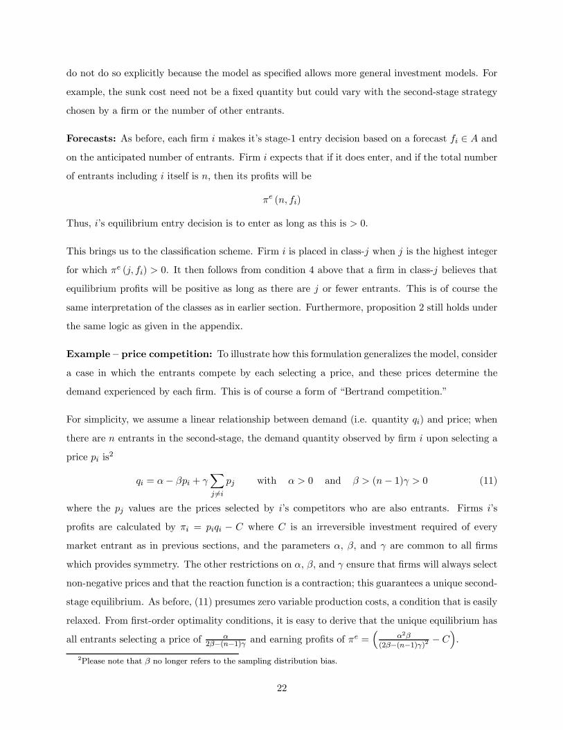
For simplicity, we assume a linear relationship between demand (i.e. quantity qi) and price; when

there are n entrants in the second-stage, the demand quantity observed by ¯rm i upon selecting a

price pi is2

qi = ®¡ ¯pi + °Xj 6=ipj with ® > 0 and ¯ > (n¡ 1)° > 0 (11)

where the pj values are the prices selected by i's competitors who are also entrants. Firms i's

pro¯ts are calculated by ¼i = piqi ¡ C where C is an irreversible investment required of every

market entrant as in previous sections, and the parameters ®, ¯, and ° are common to all ¯rms

which provides symmetry. The other restrictions on ®, ¯, and ° ensure that ¯rms will always select

non-negative prices and that the reaction function is a contraction; this guarantees a unique second-

stage equilibrium. As before, (11) presumes zero variable production costs, a condition that is easily

relaxed. From ¯rst-order optimality conditions, it is easy to derive that the unique equilibrium has

all entrants selecting a price of ®2¯¡(n¡1)° and earning pro¯ts of ¼

e =³

®2¯

(2¯¡(n¡1)°)2 ¡ C´.

2Please note that ¯ no longer refers to the sampling distribution bias.

22

In the quantity competition of previous sections, the demand parameters of equation (1) remain

constant as the number of entrants changes. In contrast, the parameters ®, ¯, and ° in (11) must

change with the number of entrants. To see why, consider a case in which there is some set of

entrants who have already reached an equilibrium in price. Now suppose that these ¯rms' prices

remain unchanged, that one more entrant is added (this will add an additional term inside the

summation of (11)), and that the parameters ®, ¯, and ° also remain unchanged. In this case (11)

tells us that the original entrants will now each sell higher quantities at the original equilibrium

price, so they will enjoy higher pro¯ts than at the original equilibrium. It can also be shown that if

the ¯rms adjust prices to reach a new equilibrium, this new equilibrium will have prices, quantities,

and pro¯ts that are greater than in the original equilibrium. In other words, we have a situation

in which a market becomes more pro¯table as it becomes less concentrated.

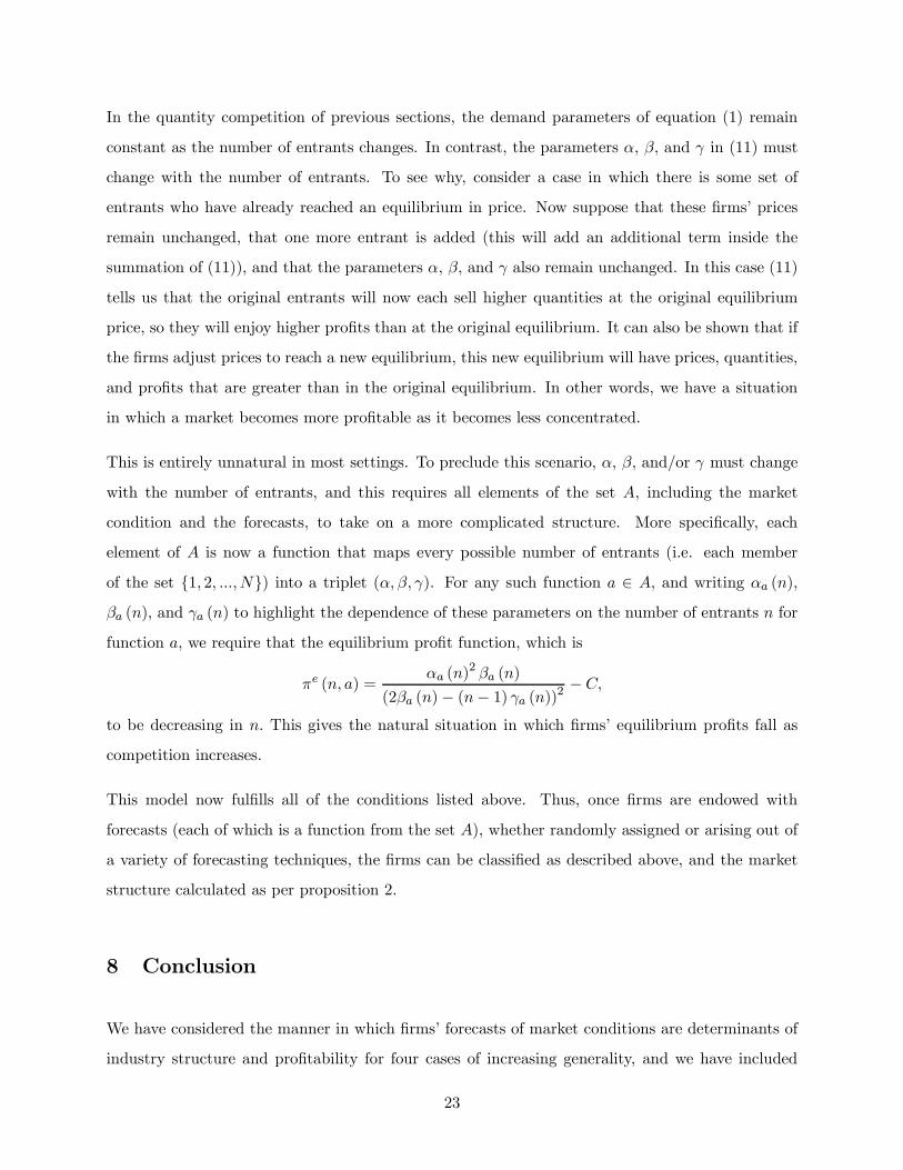
This is entirely unnatural in most settings. To preclude this scenario, ®, ¯, and/or ° must change

with the number of entrants, and this requires all elements of the set A, including the market

condition and the forecasts, to take on a more complicated structure. More speci¯cally, each

element of A is now a function that maps every possible number of entrants (i.e. each member

of the set f1; 2; :::;Ng) into a triplet (®; ¯; °). For any such function a 2 A, and writing ®a (n),¯a (n), and °a (n) to highlight the dependence of these parameters on the number of entrants n for

function a, we require that the equilibrium pro¯t function, which is

¼e (n; a) =®a (n)

2 ¯a (n)

(2¯a (n)¡ (n¡ 1) °a (n))2¡ C;

to be decreasing in n: This gives the natural situation in which ¯rms' equilibrium pro¯ts fall as

competition increases.

This model now ful¯lls all of the conditions listed above. Thus, once ¯rms are endowed with

forecasts (each of which is a function from the set A), whether randomly assigned or arising out of

a variety of forecasting techniques, the ¯rms can be classi¯ed as described above, and the market

structure calculated as per proposition 2.

8 Conclusion

We have considered the manner in which ¯rms' forecasts of market conditions are determinants of

industry structure and pro¯tability for four cases of increasing generality, and we have included

23

cases of both deterministic and probabilistic forecasts. We show with analysis and example that

industry structure and pro¯tability can be computed by a straightforward scheme of classifying

¯rms based on their beliefs about the size of the oligopoly that an emerging market can support.

Furthermore, this scheme is adaptable to quite general assumptions including randomly assigned

forecasts, forecasts that are themselves random, and di®erent modes of competition including price-

setting or Bertrand competition. It is also robust to changes in the underlying game-theoretic

assumptions; for example, we may relax the assumption of simultaneous entry decisions without

abandoning the insights drawn from the various models of this work.

We also consider the manner in which industry structure and pro¯tability change with the under-

lying problem parameters, the number of ¯rms, the nature of the ¯rms' forecasts, and the manner

in which the forecasts are dispersed or scattered.

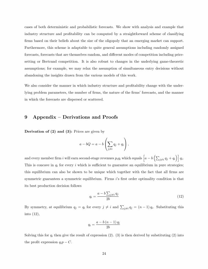
9 Appendix { Derivations and Proofs

Derivation of (2) and (3): Prices are given by

a¡ bQ = a¡ b0@Xj 6=i

qj + qi

1A ;and every member ¯rm i will earn second-stage revenues piqi which equals

ha¡ b

³Pj 6=i qj + qi

´iqi.

This is concave in qi for every i which is su±cient to guarantee an equilibrium in pure strategies;

this equilibrium can also be shown to be unique which together with the fact that all ¯rms are

symmetric guarantees a symmetric equilibrium. Firms i's ¯rst order optimality condition is that

its best production decision follows

qi =a¡ bPj 6=i qj

2b(12)

By symmetry, at equilibrium qj = qi for every j 6= i andPj 6=i qj = (n¡ 1) qi. Substituting this

into (12),

qi =a¡ b (n¡ 1) qi

2b

Solving this for qi then give the result of expression (2). (3) is then derived by substituting (2) into

the pro¯t expression qip¡ C.

24

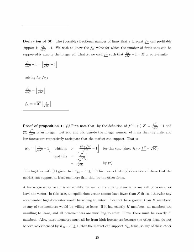
Derivation of (6): The (possibly) fractional number of ¯rms that a forecast fK can pro¯table

support isfKpbC¡ 1. We wish to know the fK value for which the number of ¯rms that can be

supported is exactly the integer K. That is, we wish fK such thatfKpbC¡ 1 = K or equivalently

fKpbC¡ 1 =

japbC¡ 1k

solving for fK :

fKpbC=j

apbC

k

fK =pbCj

apbC

k

Proof of proposition 1: (i) First note that, by the de¯nition of fK : (1) K =fKpbC¡ 1 and

(2)fKpbCis an integer. Let Khi and Klo denote the integer number of ¯rms that the high- and

low-forecasters respectively anticipate that the market can support. That is

Khi =jfhipbC¡ 1

kwhich is >

¹fK+

pbCp

bC¡ 1º

for this case (since fhi > fK +

pbC)

and this =jfKpbC

k=

fKpbC

by (2)

This together with (1) gives that Khi ¡K ¸ 1. This means that high-forecasters believe that themarket can support at least one more ¯rm than do the other ¯rms.

A ¯rst-stage entry vector is an equilibrium vector if and only if no ¯rms are willing to enter or

leave the vector. In this case, an equilibrium vector cannot have fewer than K ¯rms, otherwise any

non-member high-forecaster would be willing to enter. It cannot have greater than K members,

or any of the members would be willing to leave. If it has exactly K members, all members are

unwilling to leave, and all non-members are unwilling to enter. Thus, there must be exactly K

members. Also, these members must all be from high-forecasters because the other ¯rms do not

believe, as evidenced by Khi¡K ¸ 1, that the market can support Khi ¯rms; so any of these other

25

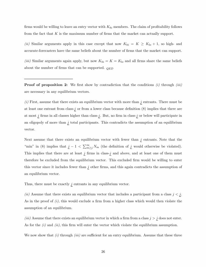
¯rms would be willing to leave an entry vector with Khi members. The claim of pro¯tability follows

from the fact that K is the maximum number of ¯rms that the market can actually support.

(ii) Similar arguments apply in this case except that now Khi = K ¸ Klo + 1, so high- and

accurate-forecasters have the same beliefs about the number of ¯rms that the market can support.

(iii) Similar arguments again apply, but now Khi = K = Klo and all ¯rms share the same beliefs

about the number of ¯rms that can be supported. QED

Proof of proposition 2: We ¯rst show by contradiction that the conditions (i) through (iii)

are necessary in any equilibrium vectors.

(i) First, assume that there exists an equilibrium vector with more than j entrants. There must be

at least one entrant from class-j or from a lower class because de¯nition (8) implies that there are

at most j ¯rms in all classes higher than class-j. But, no ¯rm in class-j or below will participate in

an oligopoly of more than j total participants. This contradicts the assumption of an equilibrium

vector.

Next assume that there exists an equilibrium vector with fewer than j entrants. Note that the

\min" in (8) implies that j ¡ 1 < P1m¸j Nm (the de¯nition of j would otherwise be violated).

This implies that there are at least j ¯rms in class-j and above, and at least one of them must

therefore be excluded from the equilibrium vector. This excluded ¯rm would be willing to enter

this vector since it includes fewer than j other ¯rms, and this again contradicts the assumption of

an equilibrium vector.

Thus, there must be exactly j entrants in any equilibrium vector.

(ii) Assume that there exists an equilibrium vector that includes a participant from a class j < j.

As in the proof of (i), this would exclude a ¯rm from a higher class which would then violate the

assumption of an equilibrium.

(iii) Assume that there exists an equilibrium vector in which a ¯rm from a class j > j does not enter.

As for the (i) and (ii), this ¯rm will enter the vector which violate the equilibrium assumption.

We now show that (i) through (iii) are su±cient for an entry equilibrium. Assume that these three

26

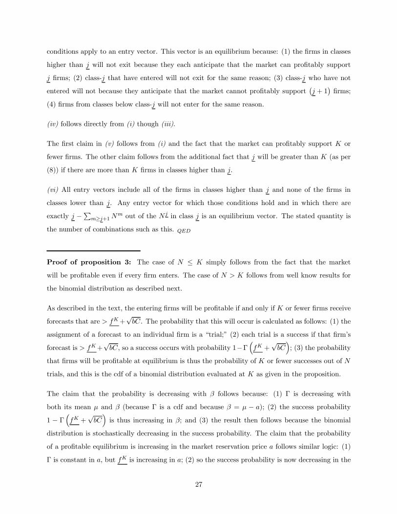
conditions apply to an entry vector. This vector is an equilibrium because: (1) the ¯rms in classes

higher than j will not exit because they each anticipate that the market can pro¯tably support

j ¯rms; (2) class-j that have entered will not exit for the same reason; (3) class-j who have not

entered will not because they anticipate that the market cannot pro¯tably support¡j + 1

¢¯rms;

(4) ¯rms from classes below class-j will not enter for the same reason.

(iv) follows directly from (i) though (iii).

The ¯rst claim in (v) follows from (i) and the fact that the market can pro¯tably support K or

fewer ¯rms. The other claim follows from the additional fact that j will be greater than K (as per

(8)) if there are more than K ¯rms in classes higher than j.

(vi) All entry vectors include all of the ¯rms in classes higher than j and none of the ¯rms in

classes lower than j. Any entry vector for which those conditions hold and in which there are

exactly j ¡Pm¸j+1Nm out of the N j in class j is an equilibrium vector. The stated quantity is

the number of combinations such as this. QED

Proof of proposition 3: The case of N · K simply follows from the fact that the market

will be pro¯table even if every ¯rm enters. The case of N > K follows from well know results for

the binomial distribution as described next.

As described in the text, the entering ¯rms will be pro¯table if and only if K or fewer ¯rms receive

forecasts that are > fK+pbC. The probability that this will occur is calculated as follows: (1) the

assignment of a forecast to an individual ¯rm is a \trial;" (2) each trial is a success if that ¯rm's

forecast is > fK+pbC, so a success occurs with probability 1¡¡

³fK +

pbC´; (3) the probability

that ¯rms will be pro¯table at equilibrium is thus the probability of K or fewer successes out of N

trials, and this is the cdf of a binomial distribution evaluated at K as given in the proposition.

The claim that the probability is decreasing with ¯ follows because: (1) ¡ is decreasing with

both its mean ¹ and ¯ (because ¡ is a cdf and because ¯ = ¹ ¡ a); (2) the success probability1 ¡ ¡

³fK +

pbC´is thus increasing in ¯; and (3) the result then follows because the binomial

distribution is stochastically decreasing in the success probability. The claim that the probability

of a pro¯table equilibrium is increasing in the market reservation price a follows similar logic: (1)

¡ is constant in a, but fK is increasing in a; (2) so the success probability is now decreasing in the

27

success probability (because ¡ is an increasing function); (3) and the result again follows because

the binomial distribution is stochastically decreasing in the success probability.

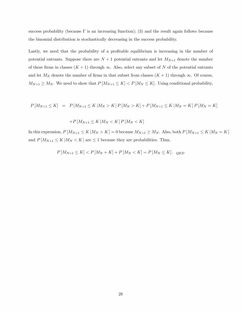
Lastly, we need that the probability of a pro¯table equilibrium is increasing in the number of

potential entrants. Suppose there are N + 1 potential entrants and let MN+1 denote the number

of these ¯rms in classes (K + 1) through 1. Also, select any subset of N of the potential entrants

and let MN denote the number of ¯rms in that subset from classes (K + 1) through 1. Of course,MN+1 ¸MN . We need to show that P [MN+1 · K] < P [MN · K]. Using conditional probability,

P [MN+1 · K] = P [MN+1 · K jMN > K ]P [MN > K] + P [MN+1 · K jMN = K ]P [MN = K]

+P [MN+1 · K jMN < K ]P [MN < K]

In this expression, P [MN+1 · K jMN > K ] = 0 becauseMN+1 ¸MN . Also, both P [MN+1 · K jMN = K ]

and P [MN+1 · K jMN < K ] are · 1 because they are probabilities. Thus,

P [MN+1 · K] < P [MN +K] + P [MN < K] = P [MN · K] : QED

28

10 References

Cachon, Gerard, and Paul Zipkin, \Competitive and Cooperative Inventory Policies in a Two-Stage

Supply Chain," Management Science, 1999, 45 (7), 936-953.

Cachon, Gerard, and Martin Lariviere, \Capacity Choice and Allocation: Strategic Behavior and

Supply Chain Performance," Management Science, 1999, 45 (8), 1091-1108.

Carr, Scott, and William Lovejoy, \The Inverse Newsvendor Problem: Choosing an Optimal De-

mand Portfolio for Capacitated Resources," Management Science, Jul 2000, 46(7), 912-927.

Carr, Scott, Izak Dueynas, and William Lovejoy, \The Harmful E®ects of Capacity Improvement,"

DOTM Working Paper 99-014, The Anderson School at UCLA, 2000.

Conlisk, John, \Why Bounded Rationality?," Journal of Economic Literature, 1996, 36, 669-700.

De Wolf, Daniel, and Yves Smeers. \A Stochastic Version of a Stackelberg-Nash-Cournot Equilib-

rium Model," Management Science, Feb 1997, 43(2), 190-197.

Dixit, Avinash, \Entry and Exit Decisions under Uncertainty," Journal of Political Economy, 1989,

97(3), 620-636.

Friedman, James W., Game Theory with Applications to Economics, 1990, Oxford University Press,

New York.

Hay, Donald and Derek Morris, Industrial Economics and Organization, 1991, Oxford University

Press, New York.

Gary-Bobo, \On the Existence of Equilibrium Points in a Class of Asymmetric Market Entry

Games," Games and Economic Behavior, 1990, 2, 239-246.

Maskin, Eric, \Uncertainty and Entry Deterence," Economic Theory, 1999, 14, 429-437.

Nahmias, Steven, Production and Operations Analysis, 1993, Irwin, Burr Ridge, IL.

Perrakis, Stylianos, and George Warskett, \Capacity and Entry Uncertainty Under Demand Un-

certainty, Review of Economic Studies, 1983, 495-511.

29

Selten and G::uth, \Equilibrium Point Selection in a Class of Market Entry Games," in Games,

Economic Dynamics, Time Series Analyis, A Symposium in Memoriam Oskar Morgenstern (M.

Deistler, E. F::urst, and G. Schw

::odiauer, Eds.), 1993, Amsterdam: North-Holland.

Sutton, John, Sunk Costs and Market Structure: Price Competition, Advertising, and the Evolution

of Concentration, 1996, MIT Press, Cambridge MA.

Van Mieghem, Jan, and Maqbool Dada, \Price Versus Production Postponement: Capacity and

Competition," Management Science, Dec 2000, 45 (12), 1631-1649.

30