Embed Size (px)
Citation preview
Proceedings World Geothermal Congress 2015
Melbourne, Australia, 19-25 April 2015
1
Flow Lognormality and Spatial Correlation in Crustal Reservoirs: II – Where-to-Drill
Guidance via Acoustic/Seismic Imaging
Peter Malin, Peter Leary, Eylon Shalev, John Rugis, Brice Valles, Carolin Boese, Jennifer Andrews & Peter Geiser
Institute of Earth Science & Engineering, University of Auckland, New Zealand
Keywords: EGS, reservoir flow, permeability stimulation, fracture stimulation, spatial correlation, lognormality
ABSTRACT
Roughly 7-10 geothermal wells are drilled in order to provide 1 well producing enough steam to drive a turbine. This well-drilling
sunk cost is, however, far from unique to geothermal reservoirs. Rather it is endemic to crustal reservoirs of all fluid types:
convention and non-conventional hydrocarbon, groundwater, fossil flow mineralisation, as well as geothermal. E.g., representative
of the vast statistical data for onshore oil field well productivity, in the year 2009 the state of Texas had 60 wells producing an
average of 645 barrels/day, 2984 wells producing an average of 88 barrels/day, and 80770 oil field wells producing an average of 1
barrel/day. As there is no intrinsic reason to consider geothermal fields significantly different from oil fields (except that the pay
fluids are different), the multi-state multi-year US oil field well producer statistics are strong indicators of how rare it is to drill
crustal reservoir 'producers': for purely blind drilling, for every geothermal producer, the intrinsic odds are for 50 non-producers
(with an additional 1300 wells that would never be considered for drilling). At $100/barrel value of oil, oil field well sunk costs are
manageable. At $1/barrel value of hot water, geothermal drilling sunk costs requires a fundamentally different well drilling
strategy. Historically geothermal wells are drilled with reference to surface manifestations and geological interpretations of
subsurface structure. Given what lognormal-distribution well productivity data tell us about the strong heterogeneity of reservoir
flow systems, we can assert that we need greatly improved subsurface flow structure data to guide the drill bit to achieve more cost-
effective hydrothermal heat extraction. We can take the necessary step by looking below the reservoir surface via innovative use of
standard multi-channel seismic sensor array technology as deployed over shale body reservoirs subjected to repeated massive
hydrofracture treatments along horizontal wellbores. Unlike oil field flow systems, which are non-flowing until disturbed by
reservoir operations, geothermal reservoir flow systems are naturally acoustically noisy, with the noise levels scaling in rough
proportion to the volume of naturally occurring fluid flow. Surface sensor array data have demonstrated that acoustic noise
generated by shale body fracking practice contain sufficient signal levels that specialised use of otherwise standard seismic
processing technology can reliably locate a large range of reservoir subsurface flow structures, most importantly the large-scale
reservoir flow patterns associated with large-scale but spatially elusive fracture channels endemic to crustal rock. While the dismal
oil field well productivity statistics amply reflects the deficiency of drilling without valid information about subsurface flow targets,
it is now possible to identify the fundamental physical reason behind poor well productivities, take technical steps to acquire
necessary reservoir flow structure information, and actively upgrade drill site locations to guide the drill bit to the main flow
structures in the reservoir fracture system.
1. INTRODUCTION
Crustal flow structures tend to be lognormally distributed. That is, in situ fluid flow tends to be dominated by a relatively small
number of large-scale/high-flux systems amidst a relatively large number of small-scale/low-flux systems. An operational
consequence of lognormally distributed in situ flow systems is that reservoir well drilling is often highly inefficient. While the
lognormal statistical features of reservoir flow have been apparent for decades, recognition of underlying physical causes, and
hence possible physics-based remedies, has been considerably slower in coming. We outline here a physical approach to in situ
flow system lognormality that provides a physics-based observational scheme for improved well-siting at geothermal reservoirs
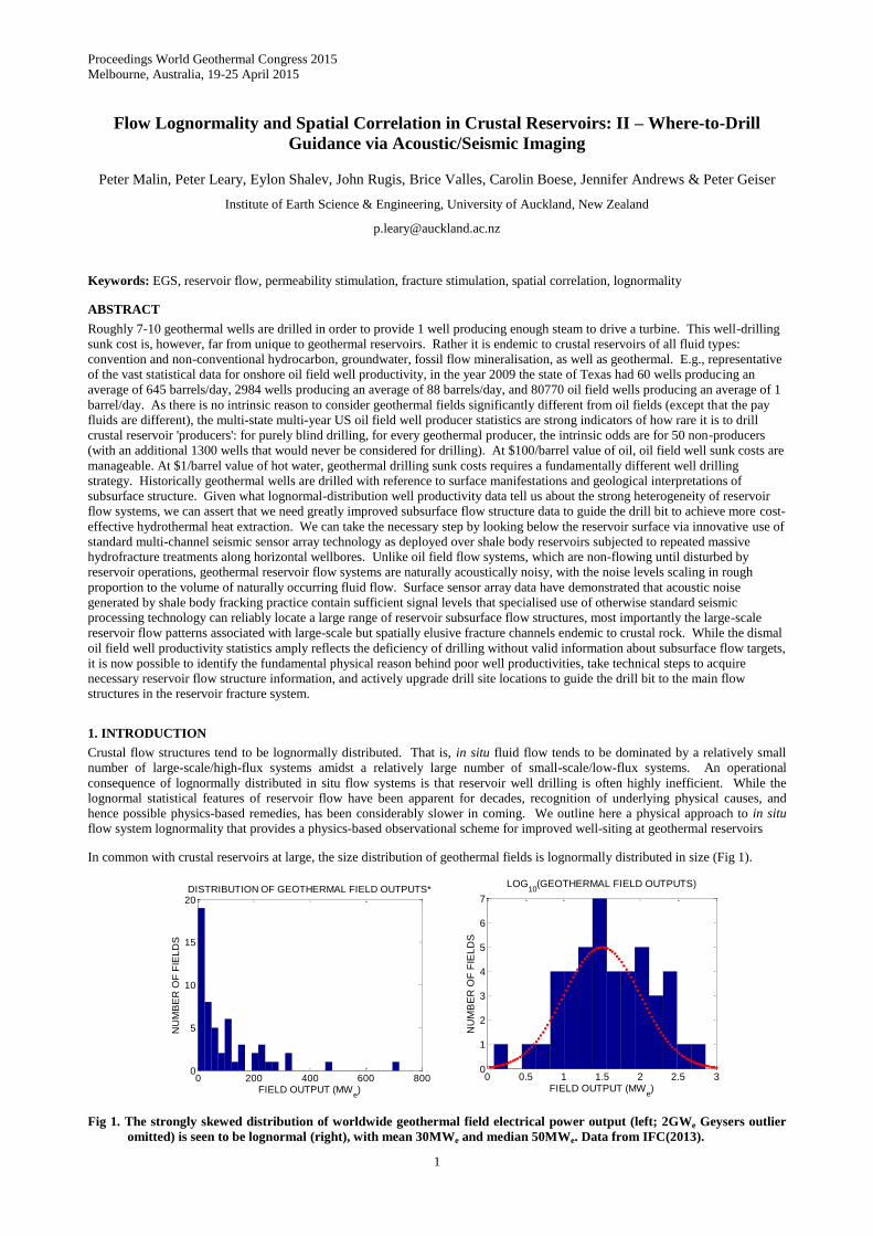
In common with crustal reservoirs at large, the size distribution of geothermal fields is lognormally distributed in size (Fig 1).
Fig 1. The strongly skewed distribution of worldwide geothermal field electrical power output (left; 2GWe Geysers outlier
omitted) is seen to be lognormal (right), with mean 30MWe and median 50MWe. Data from IFC(2013).
0 200 400 600 8000
5
10
15
20DISTRIBUTION OF GEOTHERMAL FIELD OUTPUTS*
FIELD OUTPUT (MWe)
NU
MB
ER
OF
FIE
LD
S
0 0.5 1 1.5 2 2.5 30
1
2
3
4
5
6
7
LOG10
(GEOTHERMAL FIELD OUTPUTS)
FIELD OUTPUT (MWe)
NU
MB
ER
OF
FIE
LD
S
Malin et al.
2
Oil/gas-field and mineral-deposit sizes have long been known to be lognormally distributed (Kaufman 1963; Ahrens 1963; Gerst
2008). Lognormal distributions are characteristic of permeability and well-flow populations within both hydrocarbon reservoirs
(Leary et al. 2012, 2014; USEIA 2011) and geothermal fields (Grant 2009; Leary et al. 2013). Further to the well flow statistics
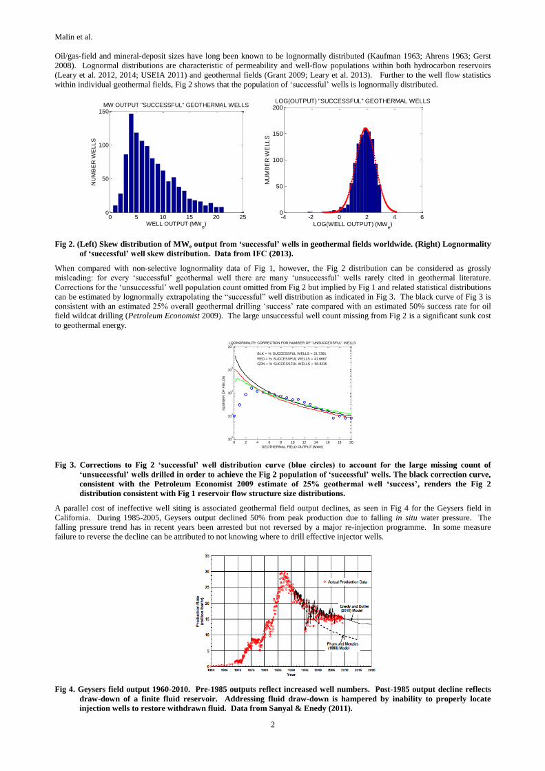
within individual geothermal fields, Fig 2 shows that the population of ‘successful’ wells is lognormally distributed.
Fig 2. (Left) Skew distribution of MWe output from ‘successful’ wells in geothermal fields worldwide. (Right) Lognormality
of ‘successful’ well skew distribution. Data from IFC (2013).
When compared with non-selective lognormality data of Fig 1, however, the Fig 2 distribution can be considered as grossly
misleading: for every ‘successful’ geothermal well there are many ‘unsuccessful’ wells rarely cited in geothermal literature.
Corrections for the ‘unsuccessful’ well population count omitted from Fig 2 but implied by Fig 1 and related statistical distributions
can be estimated by lognormally extrapolating the “successful” well distribution as indicated in Fig 3. The black curve of Fig 3 is
consistent with an estimated 25% overall geothermal drilling ‘success’ rate compared with an estimated 50% success rate for oil
field wildcat drilling (Petroleum Economist 2009). The large unsuccessful well count missing from Fig 2 is a significant sunk cost
to geothermal energy.
Fig 3. Corrections to Fig 2 ‘successful’ well distribution curve (blue circles) to account for the large missing count of
‘unsuccessful’ wells drilled in order to achieve the Fig 2 population of ‘successful’ wells. The black correction curve,
consistent with the Petroleum Economist 2009 estimate of 25% geothermal well ‘success’, renders the Fig 2
distribution consistent with Fig 1 reservoir flow structure size distributions.
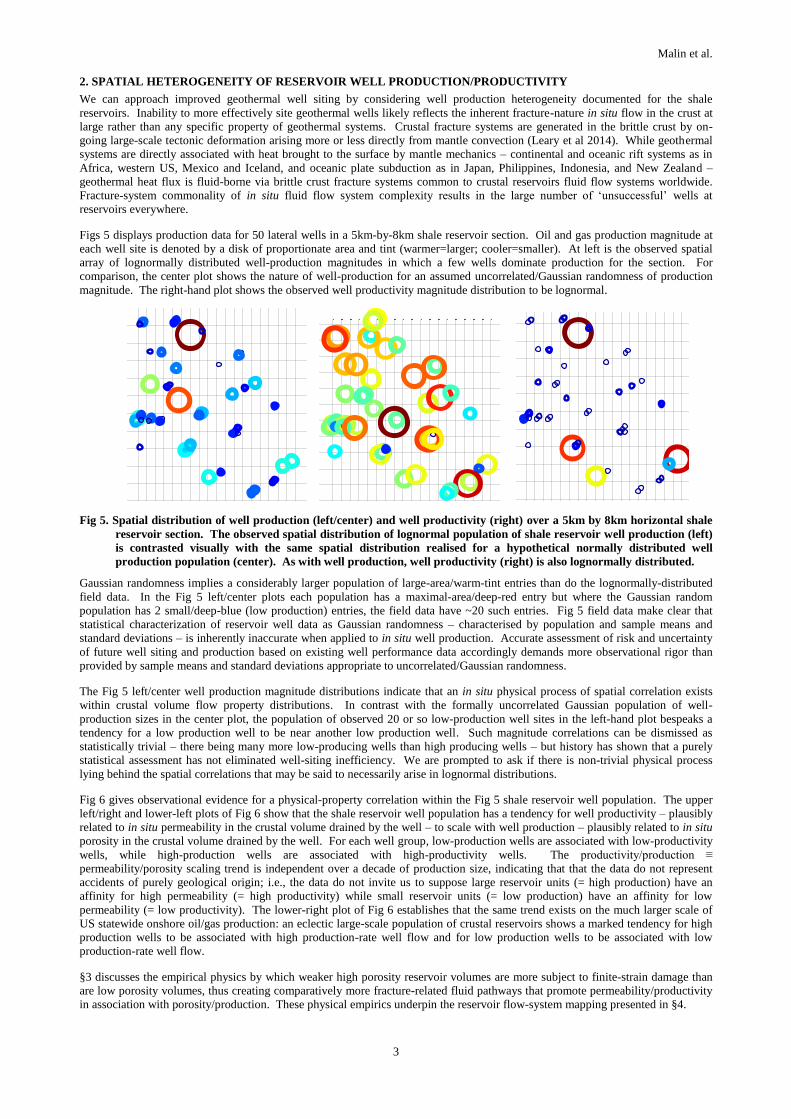
A parallel cost of ineffective well siting is associated geothermal field output declines, as seen in Fig 4 for the Geysers field in
California. During 1985-2005, Geysers output declined 50% from peak production due to falling in situ water pressure. The
falling pressure trend has in recent years been arrested but not reversed by a major re-injection programme. In some measure
failure to reverse the decline can be attributed to not knowing where to drill effective injector wells.
Fig 4. Geysers field output 1960-2010. Pre-1985 outputs reflect increased well numbers. Post-1985 output decline reflects
draw-down of a finite fluid reservoir. Addressing fluid draw-down is hampered by inability to properly locate
injection wells to restore withdrawn fluid. Data from Sanyal & Enedy (2011).
0 5 10 15 20 250
50
100
150
WELL OUTPUT (MWe)
NU
MB
ER
WE
LL
S
MW OUTPUT "SUCCESSFUL" GEOTHERMAL WELLS
-4 -2 0 2 4 60
50
100
150
200
LOG(WELL OUTPUT) (MWe)
NU
MB
ER
WE
LL
S
LOG(OUTPUT) "SUCCESSFUL" GEOTHERMAL WELLS
0 2 4 6 8 10 12 14 16 18 2010
0
101
102
103
104
GEOTHERMAL FIELD OUTPUT (MWe)
NU
MB
ER
OF
FIE
LD
S
LOGNORMALITY CORRECTION FOR NUMBER OF "UNSUCCESSFUL" WELLS
BLK = % SUCCESSFUL WELLS = 21.7391
RED = % SUCCESSFUL WELLS = 41.6667
GRN = % SUCCESSFUL WELLS = 58.8235
Malin et al.
3
2. SPATIAL HETEROGENEITY OF RESERVOIR WELL PRODUCTION/PRODUCTIVITY
We can approach improved geothermal well siting by considering well production heterogeneity documented for the shale
reservoirs. Inability to more effectively site geothermal wells likely reflects the inherent fracture-nature in situ flow in the crust at
large rather than any specific property of geothermal systems. Crustal fracture systems are generated in the brittle crust by on-
going large-scale tectonic deformation arising more or less directly from mantle convection (Leary et al 2014). While geothermal
systems are directly associated with heat brought to the surface by mantle mechanics – continental and oceanic rift systems as in
Africa, western US, Mexico and Iceland, and oceanic plate subduction as in Japan, Philippines, Indonesia, and New Zealand –
geothermal heat flux is fluid-borne via brittle crust fracture systems common to crustal reservoirs fluid flow systems worldwide.
Fracture-system commonality of in situ fluid flow system complexity results in the large number of ‘unsuccessful’ wells at
reservoirs everywhere.
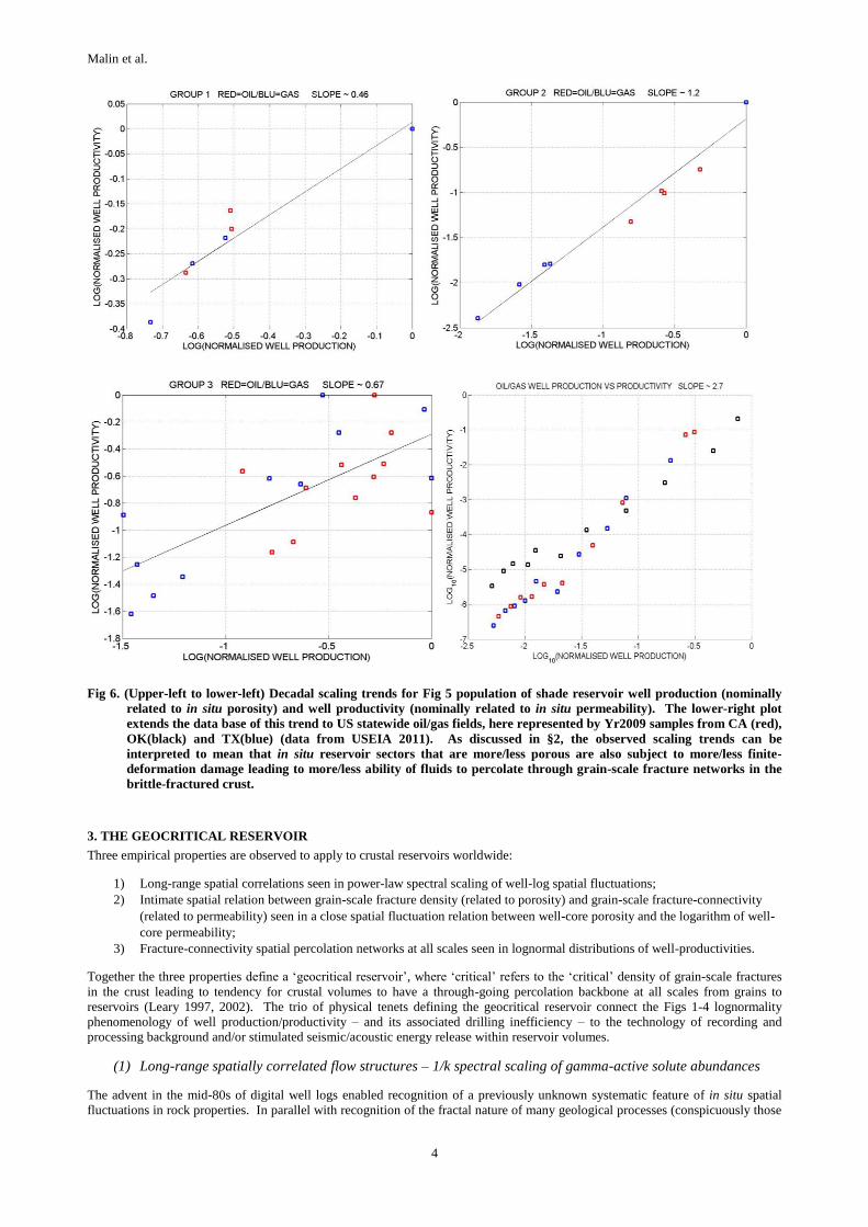
Figs 5 displays production data for 50 lateral wells in a 5km-by-8km shale reservoir section. Oil and gas production magnitude at
each well site is denoted by a disk of proportionate area and tint (warmer=larger; cooler=smaller). At left is the observed spatial
array of lognormally distributed well-production magnitudes in which a few wells dominate production for the section. For
comparison, the center plot shows the nature of well-production for an assumed uncorrelated/Gaussian randomness of production
magnitude. The right-hand plot shows the observed well productivity magnitude distribution to be lognormal.
Fig 5. Spatial distribution of well production (left/center) and well productivity (right) over a 5km by 8km horizontal shale
reservoir section. The observed spatial distribution of lognormal population of shale reservoir well production (left)
is contrasted visually with the same spatial distribution realised for a hypothetical normally distributed well
production population (center). As with well production, well productivity (right) is also lognormally distributed.
Gaussian randomness implies a considerably larger population of large-area/warm-tint entries than do the lognormally-distributed
field data. In the Fig 5 left/center plots each population has a maximal-area/deep-red entry but where the Gaussian random
population has 2 small/deep-blue (low production) entries, the field data have ~20 such entries. Fig 5 field data make clear that
statistical characterization of reservoir well data as Gaussian randomness – characterised by population and sample means and
standard deviations – is inherently inaccurate when applied to in situ well production. Accurate assessment of risk and uncertainty
of future well siting and production based on existing well performance data accordingly demands more observational rigor than
provided by sample means and standard deviations appropriate to uncorrelated/Gaussian randomness.
The Fig 5 left/center well production magnitude distributions indicate that an in situ physical process of spatial correlation exists
within crustal volume flow property distributions. In contrast with the formally uncorrelated Gaussian population of well-
production sizes in the center plot, the population of observed 20 or so low-production well sites in the left-hand plot bespeaks a
tendency for a low production well to be near another low production well. Such magnitude correlations can be dismissed as
statistically trivial – there being many more low-producing wells than high producing wells – but history has shown that a purely
statistical assessment has not eliminated well-siting inefficiency. We are prompted to ask if there is non-trivial physical process
lying behind the spatial correlations that may be said to necessarily arise in lognormal distributions.
Fig 6 gives observational evidence for a physical-property correlation within the Fig 5 shale reservoir well population. The upper
left/right and lower-left plots of Fig 6 show that the shale reservoir well population has a tendency for well productivity – plausibly
related to in situ permeability in the crustal volume drained by the well – to scale with well production – plausibly related to in situ
porosity in the crustal volume drained by the well. For each well group, low-production wells are associated with low-productivity
wells, while high-production wells are associated with high-productivity wells. The productivity/production ≡
permeability/porosity scaling trend is independent over a decade of production size, indicating that that the data do not represent
accidents of purely geological origin; i.e., the data do not invite us to suppose large reservoir units (= high production) have an
affinity for high permeability (= high productivity) while small reservoir units (= low production) have an affinity for low
permeability (= low productivity). The lower-right plot of Fig 6 establishes that the same trend exists on the much larger scale of
US statewide onshore oil/gas production: an eclectic large-scale population of crustal reservoirs shows a marked tendency for high
production wells to be associated with high production-rate well flow and for low production wells to be associated with low
production-rate well flow.
§3 discusses the empirical physics by which weaker high porosity reservoir volumes are more subject to finite-strain damage than
are low porosity volumes, thus creating comparatively more fracture-related fluid pathways that promote permeability/productivity
in association with porosity/production. These physical empirics underpin the reservoir flow-system mapping presented in §4.
-3.5-3-2.5-2-1.5-1-0.5 00.5 11.5 22.5 33.5 44.5 55.5
-5.5
-4.5
-3.5
-2.5
-1.5
-0.5
0.5
1.5
2.5
3.5
4.5
5.5
-3.5-3-2.5-2-1.5-1-0.5 00.5 11.5 22.5 33.5 44.5 55.5
-5.5
-4.5
-3.5
-2.5
-1.5
-0.5
0.5
1.5
2.5
3.5
4.5
5.5
-3.5-3-2.5-2-1.5-1-0.5 00.5 11.5 22.5 33.5 44.5 55.5
-5.5
-4.5
-3.5
-2.5
-1.5
-0.5
0.5
1.5
2.5
3.5
4.5
5.5
Malin et al.
4
Fig 6. (Upper-left to lower-left) Decadal scaling trends for Fig 5 population of shade reservoir well production (nominally
related to in situ porosity) and well productivity (nominally related to in situ permeability). The lower-right plot
extends the data base of this trend to US statewide oil/gas fields, here represented by Yr2009 samples from CA (red),
OK(black) and TX(blue) (data from USEIA 2011). As discussed in §2, the observed scaling trends can be
interpreted to mean that in situ reservoir sectors that are more/less porous are also subject to more/less finite-
deformation damage leading to more/less ability of fluids to percolate through grain-scale fracture networks in the
brittle-fractured crust.
3. THE GEOCRITICAL RESERVOIR
Three empirical properties are observed to apply to crustal reservoirs worldwide:
1) Long-range spatial correlations seen in power-law spectral scaling of well-log spatial fluctuations;
2) Intimate spatial relation between grain-scale fracture density (related to porosity) and grain-scale fracture-connectivity
(related to permeability) seen in a close spatial fluctuation relation between well-core porosity and the logarithm of well-
core permeability;
3) Fracture-connectivity spatial percolation networks at all scales seen in lognormal distributions of well-productivities.
Together the three properties define a ‘geocritical reservoir’, where ‘critical’ refers to the ‘critical’ density of grain-scale fractures
in the crust leading to tendency for crustal volumes to have a through-going percolation backbone at all scales from grains to
reservoirs (Leary 1997, 2002). The trio of physical tenets defining the geocritical reservoir connect the Figs 1-4 lognormality
phenomenology of well production/productivity – and its associated drilling inefficiency – to the technology of recording and
processing background and/or stimulated seismic/acoustic energy release within reservoir volumes.
(1) Long-range spatially correlated flow structures – 1/k spectral scaling of gamma-active solute abundances
The advent in the mid-80s of digital well logs enabled recognition of a previously unknown systematic feature of in situ spatial
fluctuations in rock properties. In parallel with recognition of the fractal nature of many geological processes (conspicuously those
Malin et al.
5
related to fractures) it was seen that the Fourier power-spectra of well logs systematically scaled inversely with spatial frequency
over five decades of scale length,
S(k) ∝ 1/kβ, β ~ 1, ~1/cm < k < ~1/km, (1)
where S(k) is the squared-amplitude or power at spatial frequency k of the spatial fluctuations measured by well-log physical
property sequence. Spectral behaviour (3) spanning grain-scales to reservoir-scales is observed to apply equally to essentially all
well-logged properties, all geological settings, and both vertical and horizontal wells (Hewett 1986; Leary 1991, 2002a; Leary et al
2013; Dolan, Bean & Riollet 1998; Marsan & Bean 1999; Shiomi, Sato & Ohtake 1997). The natural interpretation of (3) is in
terms of fractures from the grain-scale to reservoir-scale in parallel with extensive documentation of the fractal nature of fractures
(e.g., King 1983; Turcotte 1986; Hirata 1989; Leary 1991), as well as the phenomenology of low-stress induced seismicity (e.g.,
Simpson 1976; Simpson & Negmatullaev 1980; Simpson, Leith & Scholz 1988; Gupta 2002), recognition that in situ seismic
scattering points to crustal fractures at all scale lengths in the brittle-fracture upper crust (Leary & Abercrombie 1994a-b; Leary
2002a-b), and the inferred existence of grain-scale stress sensitivity evidenced by stress-aligned seismic anisotropy everywhere
(Crampin 1994) and intrinsic seismic attenuation via grain-grain contact stresses (Leary 1995).
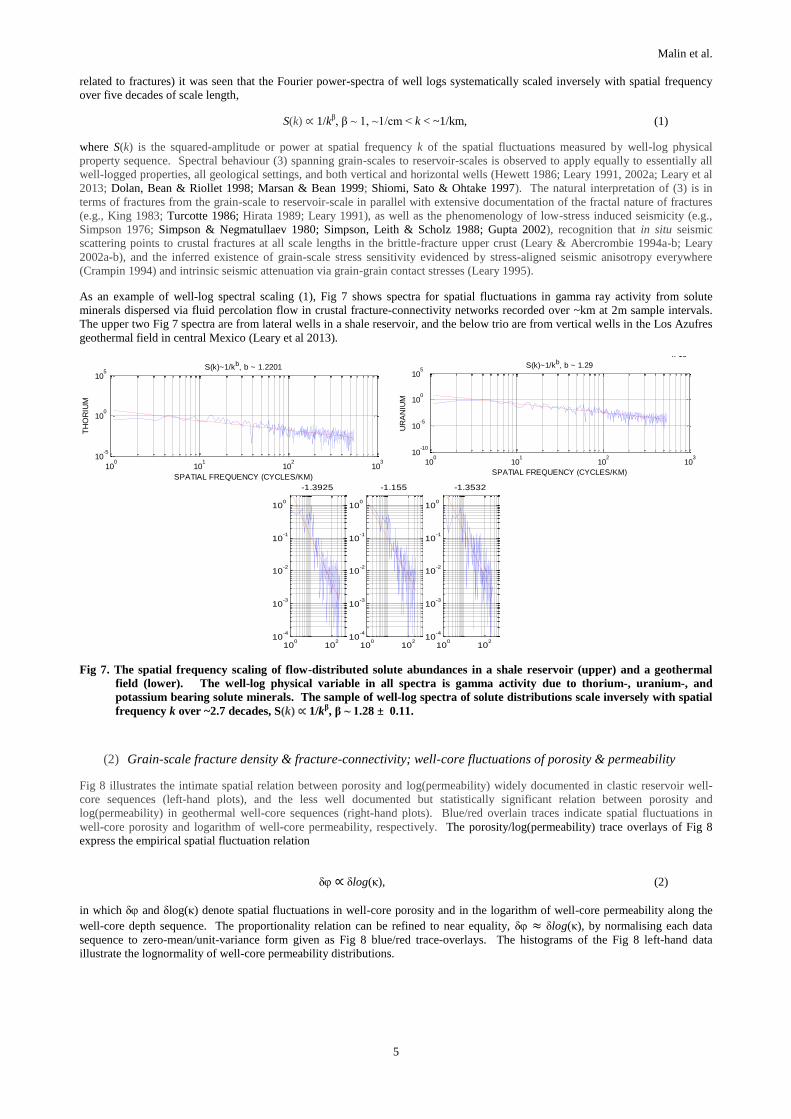
As an example of well-log spectral scaling (1), Fig 7 shows spectra for spatial fluctuations in gamma ray activity from solute
minerals dispersed via fluid percolation flow in crustal fracture-connectivity networks recorded over ~km at 2m sample intervals.
The upper two Fig 7 spectra are from lateral wells in a shale reservoir, and the below trio are from vertical wells in the Los Azufres
geothermal field in central Mexico (Leary et al 2013).
Fig 7. The spatial frequency scaling of flow-distributed solute abundances in a shale reservoir (upper) and a geothermal
field (lower). The well-log physical variable in all spectra is gamma activity due to thorium-, uranium-, and
potassium bearing solute minerals. The sample of well-log spectra of solute distributions scale inversely with spatial
frequency k over ~2.7 decades, S(k) ∝ 1/kβ, β ~ 1.28 ± 0.11.
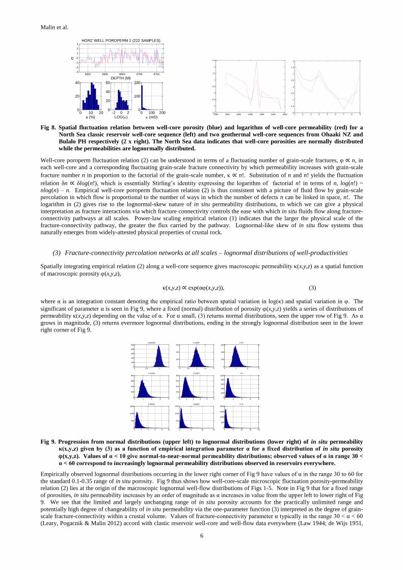
(2) Grain-scale fracture density & fracture-connectivity; well-core fluctuations of porosity & permeability
Fig 8 illustrates the intimate spatial relation between porosity and log(permeability) widely documented in clastic reservoir well-
core sequences (left-hand plots), and the less well documented but statistically significant relation between porosity and
log(permeability) in geothermal well-core sequences (right-hand plots). Blue/red overlain traces indicate spatial fluctuations in
well-core porosity and logarithm of well-core permeability, respectively. The porosity/log(permeability) trace overlays of Fig 8
express the empirical spatial fluctuation relation
δ ∝ δlog(κ), (2)
in which δ and δlog(κ) denote spatial fluctuations in well-core porosity and in the logarithm of well-core permeability along the
well-core depth sequence. The proportionality relation can be refined to near equality, δ ≈ δlog(κ), by normalising each data
sequence to zero-mean/unit-variance form given as Fig 8 blue/red trace-overlays. The histograms of the Fig 8 left-hand data
illustrate the lognormality of well-core permeability distributions.
0.85 0.9 0.95 1 1.05 1.1 1.15 1.2
x 104
0
50
100FOX-CREEK-RANCH-A1H
TH
OR
IUM
DEPTH (FT)
100
101
102
103
10-5
100
105
TH
OR
IUM
S(k)~1/kb, b ~ 1.2201
SPATIAL FREQUENCY (CYCLES/KM)
0.85 0.9 0.95 1 1.05 1.1 1.15 1.2
x 104
0
10
20
30
40FOX-CREEK-RANCH-A1H
UR
AN
IUM
DEPTH (FT)
100
101
102
103
10-10
10-5
100
105
UR
AN
IUM
S(k)~1/kb, b ~ 1.29
SPATIAL FREQUENCY (CYCLES/KM)
100
102
10-4
10-3
10-2
10-1
100
-1.3925
100
102
10-4
10-3
10-2
10-1
100
-1.155
100
102
10-4
10-3
10-2
10-1
100
-1.3532
Malin et al.
6
Fig 8. Spatial fluctuation relation between well-core porosity (blue) and logarithm of well-core permeability (red) for a
North Sea classic reservoir well-core sequence (left) and two geothermal well-core sequences from Ohaaki NZ and
Bulalo PH respectively (2 x right). The North Sea data indicates that well-core porosities are normally distributed
while the permeabilities are lognormally distributed.
Well-core poroperm fluctuation relation (2) can be understood in terms of a fluctuating number of grain-scale fractures, φ ∝ n, in
each well-core and a corresponding fluctuating grain-scale fracture connectivity by which permeability increases with grain-scale
fracture number n in proportion to the factorial of the grain-scale number, κ ∝ n!. Substitution of n and n! yields the fluctuation
relation δn ∝ δlog(n!), which is essentially Stirling’s identity expressing the logarithm of factorial n! in terms of n, log(n!) ~
nlog(n) – n. Empirical well-core poroperm fluctuation relation (2) is thus consistent with a picture of fluid flow by grain-scale
percolation in which flow is proportional to the number of ways in which the number of defects n can be linked in space, n!. The
logarithm in (2) gives rise to the lognormal-skew nature of in situ permeability distributions, to which we can give a physical
interpretation as fracture interactions via which fracture connectivity controls the ease with which in situ fluids flow along fracture-
connectivity pathways at all scales. Power-law scaling empirical relation (1) indicates that the larger the physical scale of the
fracture-connectivity pathway, the greater the flux carried by the pathway. Lognormal-like skew of in situ flow systems thus
naturally emerges from widely-attested physical properties of crustal rock.
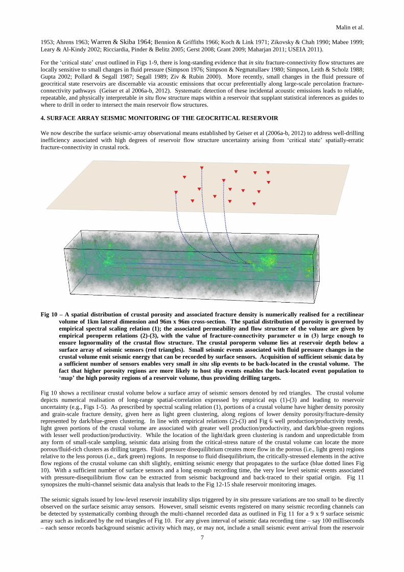
(3) Fracture-connectivity percolation networks at all scales – lognormal distributions of well-productivities
Spatially integrating empirical relation (2) along a well-core sequence gives macroscopic permeability κ(x,y,z) as a spatial function
of macroscopic porosity (x,y,z),
κ(x,y,z) ∝ exp(α(x,y,z)), (3)
where α is an integration constant denoting the empirical ratio between spatial variation in log(κ) and spatial variation in . The
significant of parameter α is seen in Fig 9, where a fixed (normal) distribution of porosity (x,y,z) yields a series of distributions of
permeability κ(x,y,z) depending on the value of α. For α small, (3) returns normal distributions, seen the upper row of Fig 9. As α
grows in magnitude, (3) returns evermore lognormal distributions, ending in the strongly lognormal distribution seen in the lower
right corner of Fig 9.
Fig 9. Progression from normal distributions (upper left) to lognormal distributions (lower right) of in situ permeability
κ(x,y,z) given by (3) as a function of empirical integration parameter α for a fixed distribution of in situ porosity
(x,y,z). Values of α < 10 give normal-to-near-normal permeability distributions; observed values of α in range 30 <
α < 60 correspond to increasingly lognormal permeability distributions observed in reservoirs everywhere.
Empirically observed lognormal distributions occurring in the lower right corner of Fig 9 have values of α in the range 30 to 60 for
the standard 0.1-0.35 range of in situ porosity. Fig 9 thus shows how well-core-scale microscopic fluctuation porosity-permeability
relation (2) lies at the origin of the macroscopic lognormal well-flow distributions of Figs 1-5. Note in Fig 9 that for a fixed range
of porosities, in situ permeability increases by an order of magnitude as α increases in value from the upper left to lower right of Fig
9. We see that the limited and largely unchanging range of in situ porosity accounts for the practically unlimited range and
potentially high degree of changeability of in situ permeability via the one-parameter function (3) interpreted as the degree of grain-
scale fracture-connectivity within a crustal volume. Values of fracture-connectivity parameter α typically in the range 30 < α < 60
(Leary, Pogacnik & Malin 2012) accord with clastic reservoir well-core and well-flow data everywhere (Law 1944; de Wijs 1951,
0 10 200
20
40
(%)-2 0 2
0
20
40
60
LOG()0 100 200
0
100
200
(mD)
8550 8600 8650 8700 8750-3
-2
-1
0
1
2
3
HORZ WELL POROPERM 1 (222 SAMPLES)
DEPTH (M)
2350 2352 2354 2356 2358 2360 2362-1.5
-1
-0.5
0
0.5
1
1.5
2
2.5
1 2 3 4 5 6 7 8 9-2
-1.5
-1
-0.5
0
0.5
1
1.5
2
0 0.5 10
100
200
300
400
5000.083333
0 0.5 1 1.5 20
200
400
6000.16667
0 1 2 30
200
400
6000.25
0 1 2 3 40
200
400
600
8000.33333
0 1 2 3 4 50
200
400
600
8000.41667
0 2 4 6 80
200
400
600
800
10000.5
0 2 4 6 8 100
500
1000
15000.58333
0 5 10 150
500
1000
15000.66667
0 5 10 15 200
500
1000
1500
20000.75
Malin et al.
7
1953; Ahrens 1963; Warren & Skiba 1964; Bennion & Griffiths 1966; Koch & Link 1971; Zikovsky & Chah 1990; Mabee 1999;
Leary & Al-Kindy 2002; Ricciardia, Pinder & Belitz 2005; Gerst 2008; Grant 2009; Maharjan 2011; USEIA 2011).
For the ‘critical state’ crust outlined in Figs 1-9, there is long-standing evidence that in situ fracture-connectivity flow structures are
locally sensitive to small changes in fluid pressure (Simpson 1976; Simpson & Negmatullaev 1980; Simpson, Leith & Scholz 1988;
Gupta 2002; Pollard & Segall 1987; Segall 1989; Ziv & Rubin 2000). More recently, small changes in the fluid pressure of
geocritical state reservoirs are discernable via acoustic emissions that occur preferentially along large-scale percolation fracture-
connectivity pathways (Geiser et al 2006a-b, 2012). Systematic detection of these incidental acoustic emissions leads to reliable,
repeatable, and physically interpretable in situ flow structure maps within a reservoir that supplant statistical inferences as guides to
where to drill in order to intersect the main reservoir flow structures.
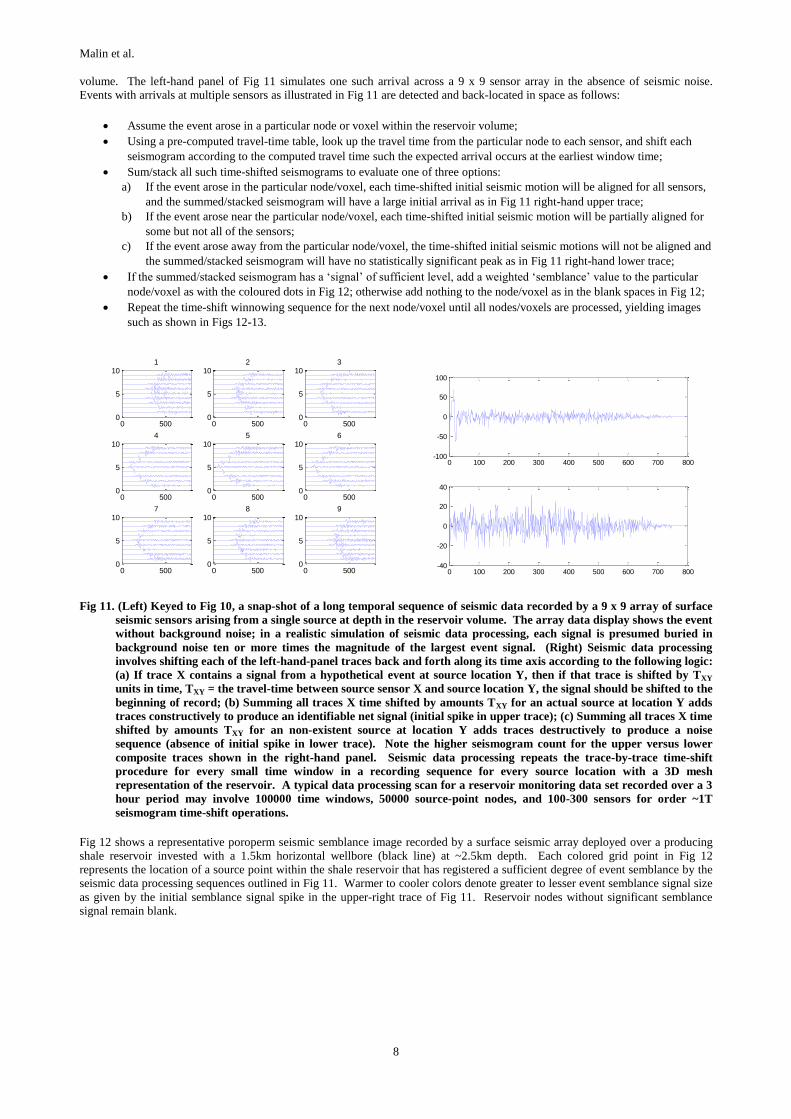
4. SURFACE ARRAY SEISMIC MONITORING OF THE GEOCRITICAL RESERVOIR
We now describe the surface seismic-array observational means established by Geiser et al (2006a-b, 2012) to address well-drilling
inefficiency associated with high degrees of reservoir flow structure uncertainty arising from ‘critical state’ spatially-erratic
fracture-connectivity in crustal rock.
Fig 10 – A spatial distribution of crustal porosity and associated fracture density is numerically realised for a rectilinear
volume of 1km lateral dimension and 96m x 96m cross-section. The spatial distribution of porosity is governed by
empirical spectral scaling relation (1); the associated permeability and flow structure of the volume are given by
empirical poroperm relations (2)-(3), with the value of fracture-connectivity parameter α in (3) large enough to
ensure lognormality of the crustal flow structure. The crustal poroperm volume lies at reservoir depth below a
surface array of seismic sensors (red triangles). Small seismic events associated with fluid pressure changes in the
crustal volume emit seismic energy that can be recorded by surface sensors. Acquisition of sufficient seismic data by
a sufficient number of sensors enables very small in situ slip events to be back-located in the crustal volume. The
fact that higher porosity regions are more likely to host slip events enables the back-located event population to
‘map’ the high porosity regions of a reservoir volume, thus providing drilling targets.
Fig 10 shows a rectilinear crustal volume below a surface array of seismic sensors denoted by red triangles. The crustal volume
depicts numerical realisation of long-range spatial-correlation expressed by empirical eqs (1)-(3) and leading to reservoir
uncertainty (e.g., Figs 1-5). As prescribed by spectral scaling relation (1), portions of a crustal volume have higher density porosity
and grain-scale fracture density, given here as light green clustering, along regions of lower density porosity/fracture-density
represented by dark/blue-green clustering. In line with empirical relations (2)-(3) and Fig 6 well production/productivity trends,
light green portions of the crustal volume are associated with greater well production/productivity, and dark/blue-green regions
with lesser well production/productivity. While the location of the light/dark green clustering is random and unpredictable from
any form of small-scale sampling, seismic data arising from the critical-stress nature of the crustal volume can locate the more
porous/fluid-rich clusters as drilling targets. Fluid pressure disequilibrium creates more flow in the porous (i.e., light green) regions
relative to the less porous (i.e., dark green) regions. In response to fluid disequilibrium, the critically-stressed elements in the active
flow regions of the crustal volume can shift slightly, emitting seismic energy that propagates to the surface (blue dotted lines Fig
10). With a sufficient number of surface sensors and a long enough recording time, the very low level seismic events associated
with pressure-disequilibrium flow can be extracted from seismic background and back-traced to their spatial origin. Fig 11
synopsizes the multi-channel seismic data analysis that leads to the Fig 12-15 shale reservoir monitoring images.
The seismic signals issued by low-level reservoir instability slips triggered by in situ pressure variations are too small to be directly
observed on the surface seismic array sensors. However, small seismic events registered on many seismic recording channels can
be detected by systematically combing through the multi-channel recorded data as outlined in Fig 11 for a 9 x 9 surface seismic
array such as indicated by the red triangles of Fig 10. For any given interval of seismic data recording time – say 100 milliseconds
– each sensor records background seismic activity which may, or may not, include a small seismic event arrival from the reservoir
Malin et al.
8
volume. The left-hand panel of Fig 11 simulates one such arrival across a 9 x 9 sensor array in the absence of seismic noise.
Events with arrivals at multiple sensors as illustrated in Fig 11 are detected and back-located in space as follows:
Assume the event arose in a particular node or voxel within the reservoir volume;
Using a pre-computed travel-time table, look up the travel time from the particular node to each sensor, and shift each
seismogram according to the computed travel time such the expected arrival occurs at the earliest window time;
Sum/stack all such time-shifted seismograms to evaluate one of three options:
a) If the event arose in the particular node/voxel, each time-shifted initial seismic motion will be aligned for all sensors,
and the summed/stacked seismogram will have a large initial arrival as in Fig 11 right-hand upper trace;
b) If the event arose near the particular node/voxel, each time-shifted initial seismic motion will be partially aligned for
some but not all of the sensors;
c) If the event arose away from the particular node/voxel, the time-shifted initial seismic motions will not be aligned and
the summed/stacked seismogram will have no statistically significant peak as in Fig 11 right-hand lower trace;
If the summed/stacked seismogram has a ‘signal’ of sufficient level, add a weighted ‘semblance’ value to the particular
node/voxel as with the coloured dots in Fig 12; otherwise add nothing to the node/voxel as in the blank spaces in Fig 12;
Repeat the time-shift winnowing sequence for the next node/voxel until all nodes/voxels are processed, yielding images
such as shown in Figs 12-13.
Fig 11. (Left) Keyed to Fig 10, a snap-shot of a long temporal sequence of seismic data recorded by a 9 x 9 array of surface
seismic sensors arising from a single source at depth in the reservoir volume. The array data display shows the event
without background noise; in a realistic simulation of seismic data processing, each signal is presumed buried in
background noise ten or more times the magnitude of the largest event signal. (Right) Seismic data processing
involves shifting each of the left-hand-panel traces back and forth along its time axis according to the following logic:
(a) If trace X contains a signal from a hypothetical event at source location Y, then if that trace is shifted by TXY
units in time, TXY = the travel-time between source sensor X and source location Y, the signal should be shifted to the
beginning of record; (b) Summing all traces X time shifted by amounts TXY for an actual source at location Y adds
traces constructively to produce an identifiable net signal (initial spike in upper trace); (c) Summing all traces X time
shifted by amounts TXY for an non-existent source at location Y adds traces destructively to produce a noise
sequence (absence of initial spike in lower trace). Note the higher seismogram count for the upper versus lower
composite traces shown in the right-hand panel. Seismic data processing repeats the trace-by-trace time-shift
procedure for every small time window in a recording sequence for every source location with a 3D mesh
representation of the reservoir. A typical data processing scan for a reservoir monitoring data set recorded over a 3
hour period may involve 100000 time windows, 50000 source-point nodes, and 100-300 sensors for order ~1T
seismogram time-shift operations.
Fig 12 shows a representative poroperm seismic semblance image recorded by a surface seismic array deployed over a producing
shale reservoir invested with a 1.5km horizontal wellbore (black line) at ~2.5km depth. Each colored grid point in Fig 12
represents the location of a source point within the shale reservoir that has registered a sufficient degree of event semblance by the
seismic data processing sequences outlined in Fig 11. Warmer to cooler colors denote greater to lesser event semblance signal size
as given by the initial semblance signal spike in the upper-right trace of Fig 11. Reservoir nodes without significant semblance
signal remain blank.
0 5000
5
101
0 5000
5
102
0 5000
5
103
0 5000
5
104
0 5000
5
105
0 5000
5
106
0 5000
5
107
0 5000
5
108
0 5000
5
109
0 100 200 300 400 500 600 700 800-100
-50
0
50
100
0 100 200 300 400 500 600 700 800-40
-20
0
20
40
Malin et al.
9
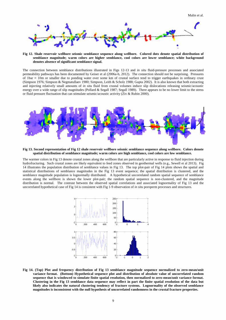
Fig 12. Shale reservoir wellbore seismic semblance sequence along wellbore. Colored dots denote spatial distribution of
semblance magnitude; warm colors are higher semblance, cool colors are lower semblance; white background
denotes absence of significant semblance signal.
The connection between semblance distributions illustrated in Figs 12-13 and in situ fluid-pressure processes and associated
permeability pathways has been documented by Geiser et al (2006a-b, 2012). The connection should not be surprising. Pressures
of 1bar ≡ 10m or smaller due to ponding water over some km of crustal surface tend to trigger earthquakes in ordinary crust
(Simpson 1976; Simpson & Negmatullaev 1980; Simpson, Leith & Scholz 1988; Gupta 2002). It is also known that both extracting
and injecting relatively small amounts of in situ fluid from crustal volumes induce slip dislocations releasing seismic/acoustic
energy over a wide range of slip magnitudes (Pollard & Segall 1987; Segall 1989). There appears to be no lower limit to the stress
or fluid pressure fluctuation that can stimulate seismic/acoustic activity (Ziv & Rubin 2000).
Fig 13. Second representation of Fig 12 shale reservoir wellbore seismic semblance sequence along wellbore. Colors denote
spatial distribution of semblance magnitude; warm colors are high semblance, cool colors are low semblance.
The warmer colors in Fig 13 denote crustal zones along the wellbore that are particularly active in response to fluid injection during
hydrofracturing. Such crustal zones are likely equivalent to feed zones observed in geothermal wells (e.g., Sewell et al 2013). Fig
14 illustrates the population distribution of semblance values in Fig 13. The top plot-pair of Fig 14 plots shows the spatial and
statistical distributions of semblance magnitudes in the Fig 13 event sequence; the spatial distribution is clustered, and the
semblance magnitude population is lognormally distributed. A hypothetical uncorrelated random spatial sequence of semblance
events along the wellbore is shown the lower plot-pair; the random spatial sequence is non-clustered, and the magnitude
distribution is normal. The contrast between the observed spatial correlations and associated lognormality of Fig 13 and the
uncorrelated hypothetical case of Fig 14 is consistent with Fig 1-9 observation of in situ poroperm processes and structures.
Fig 14. (Top) Plot and frequency distribution of Fig 13 semblance magnitude sequence normalized to zero-mean/unit
variance format. (Bottom) Hypothetical sequence plot and distribution of absolute value of uncorrelated random
sequence that is windowed to simulate finite spatial resolution, then normalized to zero-mean/unit variance format.
Clustering in the Fig 13 semblance data sequence may reflect in part the finite spatial resolution of the data but
likely also indicates the natural clustering tendency of fracture systems. Lognormality of the observed semblance
magnitudes is inconsistent with the null hypothesis of uncorrelated randomness in the crustal fracture properties.
-2 0 2 40
50
100
150
200
250
0 200 400 600-2
0
2
4
-2 -1 0 1 20
20
40
60
80
0 200 400 600-1
-0.5
0
0.5
1
Malin et al.
10
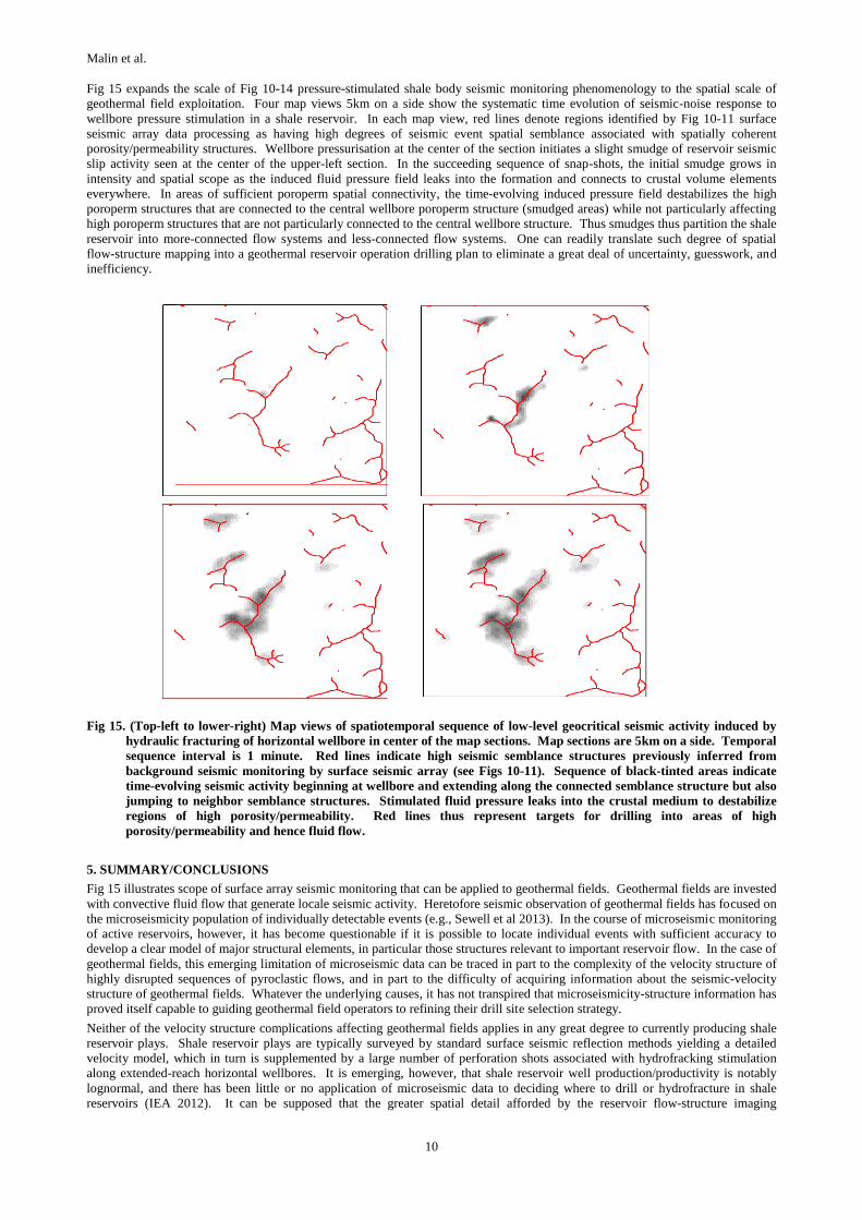
Fig 15 expands the scale of Fig 10-14 pressure-stimulated shale body seismic monitoring phenomenology to the spatial scale of
geothermal field exploitation. Four map views 5km on a side show the systematic time evolution of seismic-noise response to
wellbore pressure stimulation in a shale reservoir. In each map view, red lines denote regions identified by Fig 10-11 surface
seismic array data processing as having high degrees of seismic event spatial semblance associated with spatially coherent
porosity/permeability structures. Wellbore pressurisation at the center of the section initiates a slight smudge of reservoir seismic
slip activity seen at the center of the upper-left section. In the succeeding sequence of snap-shots, the initial smudge grows in
intensity and spatial scope as the induced fluid pressure field leaks into the formation and connects to crustal volume elements
everywhere. In areas of sufficient poroperm spatial connectivity, the time-evolving induced pressure field destabilizes the high
poroperm structures that are connected to the central wellbore poroperm structure (smudged areas) while not particularly affecting
high poroperm structures that are not particularly connected to the central wellbore structure. Thus smudges thus partition the shale
reservoir into more-connected flow systems and less-connected flow systems. One can readily translate such degree of spatial
flow-structure mapping into a geothermal reservoir operation drilling plan to eliminate a great deal of uncertainty, guesswork, and
inefficiency.
Fig 15. (Top-left to lower-right) Map views of spatiotemporal sequence of low-level geocritical seismic activity induced by
hydraulic fracturing of horizontal wellbore in center of the map sections. Map sections are 5km on a side. Temporal
sequence interval is 1 minute. Red lines indicate high seismic semblance structures previously inferred from
background seismic monitoring by surface seismic array (see Figs 10-11). Sequence of black-tinted areas indicate
time-evolving seismic activity beginning at wellbore and extending along the connected semblance structure but also
jumping to neighbor semblance structures. Stimulated fluid pressure leaks into the crustal medium to destabilize
regions of high porosity/permeability. Red lines thus represent targets for drilling into areas of high
porosity/permeability and hence fluid flow.
5. SUMMARY/CONCLUSIONS
Fig 15 illustrates scope of surface array seismic monitoring that can be applied to geothermal fields. Geothermal fields are invested
with convective fluid flow that generate locale seismic activity. Heretofore seismic observation of geothermal fields has focused on
the microseismicity population of individually detectable events (e.g., Sewell et al 2013). In the course of microseismic monitoring
of active reservoirs, however, it has become questionable if it is possible to locate individual events with sufficient accuracy to
develop a clear model of major structural elements, in particular those structures relevant to important reservoir flow. In the case of
geothermal fields, this emerging limitation of microseismic data can be traced in part to the complexity of the velocity structure of
highly disrupted sequences of pyroclastic flows, and in part to the difficulty of acquiring information about the seismic-velocity
structure of geothermal fields. Whatever the underlying causes, it has not transpired that microseismicity-structure information has
proved itself capable to guiding geothermal field operators to refining their drill site selection strategy.
Neither of the velocity structure complications affecting geothermal fields applies in any great degree to currently producing shale
reservoir plays. Shale reservoir plays are typically surveyed by standard surface seismic reflection methods yielding a detailed
velocity model, which in turn is supplemented by a large number of perforation shots associated with hydrofracking stimulation
along extended-reach horizontal wellbores. It is emerging, however, that shale reservoir well production/productivity is notably
lognormal, and there has been little or no application of microseismic data to deciding where to drill or hydrofracture in shale
reservoirs (IEA 2012). It can be supposed that the greater spatial detail afforded by the reservoir flow-structure imaging

Malin et al.
11
demonstrated by Geiser et al (2006a-b, 2012) for surface-sensor array event detection and location will address the fundamental
limitations of reliable flow-structure information endemic to microseismicity data.
The present discussion recasts seismic monitoring of geothermal fields in terms of low-level seismic event semblance images to
take advantage of the high level of background noise that is fundamentally coupled to in situ fluid flow structures. This imaging
process requires investment in acquiring velocity models of unprecedented accuracy for geothermal fields. There is no reason to
believe, however, that the steady history of ever-increasing seismic array channel count leading to ever-increasing seismic imaging
accuracy and fidelity in standard geological formations cannot be adapted to a geothermal setting by suitably adapting the multi-
channel data processing capability of surface seismic imaging. Heretofore seismic imaging of geothermal fields has been limited to
either low-event-count microseismic data or to surface sourcing. Low-level seismic event semblance imaging addresses both these
prior imaging deficiencies. Low-level seismic event noise generation in geothermal areas is fundamentally coupled to the precise
flow-structure observations that are sought. Sources of significance are naturally occurring at depth rather than assembled to
operate at the surface. Refraction seismic sourcing into a dense surface sensor array can generate essentially arbitrarily accurate
velocity models by which to process surface seismic array data. Seismic array listening time is an essentially low cost means to
increased spatial resolution. For initial purposes, the subsurface spatial resolution problem is considerably relaxed from that
associated with current shale reservoir practice. Identifying/locating in situ flow structures at a voxel resolution of 25m-50m would
give a huge boost to drilling confidence at a tiny fraction of cost of a single well, let alone multiple wells. Subsequent detailed
seismic semblance imaging of particular areas could likely refine the voxel resolution to more accurately guide drill siting to
precisely the in situ flow-active targets demanded by geothermal power production.
Accompanying Papers I (Leary et al. 2015) & III (Pogacnik et al. 2015) have as their joint theme the strong limitation of thermal
conductivity on EGS as a source of commercial heat energy. Central to the arguments of I & III is the importance of achieving
advective flow in the larger context of ultimate conductive thermal recharge of crustal heat exchange volumes. This perspective is
informed by noting, as in I, that virtually all commercial geothermal heat energy extraction occurs in connection with in situ
convective (advective) flow systems. For EGS as primarily focused on conduction-limited crustal heat resource, this puts a
premium on creating interior advective flow systems matched to exterior conductive recharge flow. But achieving this result for
EGS crustal volumes confronts the same problems of complex, heterogeneous, spatially erratic in situ flow processes here
addressed re better drill site targeting for better use of hydrothermal flow system resources. If, as seems probable, growth of
geothermal energy acquisition and use in the immediate future lies in improved use of existing/proven resources, we can expect to
use the reservoir imaging technology outlined here in the largest possible geothermal energy context:
Reversing the steady decline of existing geothermal fields;
Extending the spatial reach of known fields;
Bringing on line more marginal fields.
Each of these goals has its own commercial worth, but together they have a larger role to play in understanding in situ flow as
physical process far more complex than hitherto understood. Making steady concerted progress in understanding present
geothermal resources can be the key to opening the future to expanded access to crustal heat.
REFERENCES
Ahrens LH (1963) Lognormal-type distributions in igneous rocks – IV, Geochmica Cosmochim Acta 27, 333-343.
Bennion DW & Griffiths JC (1966) A stochastic model for predicting variations in reservoir rock properties, Soc. Petrol. Eng.
Jour., Trans. ATME 237, 9-16.
Crampin S (1994) The fracture criticality of crustal rocks, Geophysical Journal International 118, 428-438.
de Wijs HJ (1951) Statistics of ore distribution. Part I: frequency distribution of assay values, J. R. Neth. Geol. Min. Soc. New Ser.
13, 365–375.
de Wijs HJ (1953) Statistics of ore distribution Part II: theory of binomial distribution applied to sampling and engineering
problems, J. R. Neth. Geol. Min. Soc. New Ser. 15, 125–124..
Dolan SS, Bean CJ & Riollet B (1998) The broadband fractal nature of heterogeneity in the upper crust from petrophysical logs,
Geophys. J. Int. 132, 489-507.
Geiser, P., J. Vermilye, R. Scammell, S. Roecker, 2006a, Seismic Emission Tomography 1: Seismic used to directly map reservoir
permeability fields: Oil & Gas Journal, v. 104, no. 46 6p.
Geiser, P., J. Vermilye, R. Scammell, S. Roecker, 2006b, Seismic Emission Tomography - 2: Seismic used to directly map
reservoir permeability fields: Oil & Gas Journal, v. 104, no. 47, 6p.
Geiser P., A. Lacazette, and J. Vermilye, 2012, Beyond ‘dots in a box’: an empirical view of reservoir permeability with
tomographic fracture imaging, First Break 30, p. 63-69.
Gerst MD (2008) Revisiting the Cumulative Grade-Tonnage Relationship for Major Copper Ore Types, Economic Geology 103,
615–628.
Grant MA (2009) Optimization of drilling acceptance criteria, Geothermics 38, 247–253.
Gupta HK (2002) A review of recent studies of triggered earthquakes by artificial water reservoirs with special emphasis on
earthquakes in Koyna, India, Earth-Science Reviews 58, 279–310.
Hewett TA (1986) Fractal distributions of reservoir heterogeneity and their influence on fluid transport, SPE Paper 15386, 61st SPE
Annual Technical Conference, New Orleans.
IFC (2013) Success of Geothermal Wells: A global study, International Finance Corporation, Washington DC, 80pp.
International Energy Agency (2012) Special Report: Golden Rules for Golden Age of Gas, International Energy Agency,
www.iea.org; http://www.iea.org/publications/ freepublications/publication/WEO2012_GoldenRulesReport.pdf, 150p.
Kaufman GM (1963) Statistical Decision and Related Techniques in Oil and Gas Exploration, Prentice-Hall, Englewood Cliffs, NJ.

Malin et al.
12
Koch GS & Link RF (1971) The coefficient of variation; a guide to the sampling of ore deposits, Economic Geology 66, 293-301.
Law J (1944) A statistical approach to the interstitial heterogeneity of sand reservoirs, Technical Publication 1732, Petroleum
Technology 7, May 1944.
Leary P, Malin P, Geiser P, Pogacnik J, Rugis J & Valles B (2015) Flow Lognormality & Spatial Correlation in Crustal Reservoirs
– I: Physical Character & Consequences for Geothermal Energy, WGC2015, 19-24 April 2015, Melbourne AU.
Leary P, Malin P, Pogacnik J, Rugis J, Valles B & Geiser P (2014) Lognormality, δκ ~ κ δφ, EGS, and all that, Proceedings 39th
Stanford Geothermal Workshop, February 24-26 2014, Stanford University, CA.
Leary PC, Malin PE, Ryan GA, Lorenzo C & Flores M (2013) Lognormally distributed K/Th/U concentrations – Evidence for
geocritical fracture flow, Los Azufres geothermal field, MX, Proceedings Geothermal Resources Council 36th Annual
Conference, 29 Sep – 3 Oct, Las Vegas NV.
Leary P, Pogacnik J & Malin P (2012) Fractures ~ Porosity --> Connectivity ~ Permeability --> EGS Flow Stimulation,
Proceedings 36th Geothermal Resources Council 36th Annual Conference, 30 Sep – 3 Oct, Reno NV.
Leary PC (2002a) Fractures and physical heterogeneity in crustal rock, in Heterogeneity of the Crust and Upper Mantle – Nature,
Scaling and Seismic Properties, J. A. Goff, & K. Holliger (eds.), Kluwer Academic/Plenum Publishers, New York, 155-186.
Leary PC (2002b) Numerical simulation of first-order backscattered P- and S-waves for time-lapse seismic imaging in
heterogeneous reservoirs, Geophysical Journal International 148, 402-425.
Leary PC (1997) Rock as a critical-point system and the inherent implausibility of reliable earthquake prediction, Geophysical
Journal International 131, 451-466.
Leary PC (1995) The cause of frequency-dependent seismic absorption in crustal rock, Geophysical Journal International 122,
143-151.
Leary PC (1991) Deep borehole log evidence for fractal distribution of fractures in crystalline rock. Geophysical Journal
International 107, 615-628.
Leary PC & Al-Kindy F (2002) Power-law scaling of spatially correlated porosity and log(permeability) sequences from north-
central North Sea Brae oilfield well core, Geophysical Journal International 148, 426-442.
Leary P & Abercrombie RE (1994a) Frequency dependent crustal scattering and absorption at 5-160 Hz from coda decay observed
at 2.5 km depth, Geophysical Research Letters 21, 971-974.
Leary P & Abercrombie RE (1994b) Fractal fracture scattering origin of S-wave coda: spectral evidence from recordings at 2.5 km,
Geophysical Research Letters 21, 1683-1686.
Mabee SB (1999) Factors influencing well productivity in glaciated metamorphic rocks, Ground Water 37, 88-97.
Maharjan M (2011) Interpretation of domestic water well production data as a tool for detection of transmissive
bedrock fractured zones under cover of the glacial formations in Geauga County, Ohio, M.S. Thesis, Kent State
University. Malin P, Leary P, Shalev E, Rugis J, Valles B, Boese C, Andrews J & Geiser P (2015) Flow Lognormality and Spatial Correlation
in Crustal Reservoirs: II – Where-to-Drill Guidance via Acoustic/Seismic Imaging, WGC2015, 19-24 April 2015, Melbourne
AU.
Marsan D & Bean CJ (1999) Multiscaling nature of sonic velocities and lithology in the upper crystalline crust: Evidence from the
KTB main borehole, Geophysical Research Letters 26, 275-278.
Petroleum Economist (2009) Unlocking the value of the world's geothermal resources, Euromoney Institutional Investor PLC,
London, UK
Pogacnik J, Leary P, Malin P, Geiser P, Rugis R & Valles B (2015) Flow Lognormality and Spatial Correlation in Crustal
Reservoirs: III -- Natural Permeability Enhancement via Biot Fluid-Rock Coupling At All Scales, WGC2015, 19-24 April
2015, Melbourne AU.
Pollard, D. D., and P. Segall, 1987, Theoretical displacements and stresses near fractures in rock with applications to faults, joints,
veins, dikes, and solution surfaces, in B. K. Atkinson, ed., Fracture Mechanics of Rock, Academic, San Diego, CA., 1987.
Ricciardia K.L., G.F. Pinder& K. Belitz , 2005. Comparison of the lognormal and beta distribution functions to describe the
uncertainty in permeability, Journal of Hydrology 313, 248-256.
Segall P., 1989, Earthquakes triggered by fluid extraction. Geology 17(10), 942–946.
Sewell SM, Cumming W, Bardsley CJ, Winick J, Quinao J, Wallis IC, Sherburn S, Bourguignon S & Bannister S (2013)
Interpretation of microearthquakes at the Rotokawa geothermal field, 2008 to 2012, Proceedings 35th New Zealand
Geothermal Workshop, Rotorua, NZ.
Simpson DW (1976) Seismicity changes associated with reservoir loading, Engineering Geology 10, 123-150.
Simpson DW & Negmatullaev SK (1980) Induced seismicity at Nurek Reservoir, Tadjikistan, USSR, Bulletin of the Seismological
Society of America 70, 1561-1586
Simpson DW, Leith WS & Scholz CH (1988) Two types of reservoir-induced seismicity, Bulletin of the Seismological Society of
America 78, 2025-2040.
Sanyal SK & Enedy SL (2011) Fifty years of power generation at the Geysers geothermal field, California – The lessons learned,
Proceedings 36th Workshop on Geothermal Reservoir Engineering, Stanford University, January 31 - February 2.
Shiomi K, Sato H & Ohtake M (1997) Broadband power-law spectra of well-log data in Japan, Geophys. J. Int. 130, 57-64.
US Energy Information Administration (2011) Distribution and Production of Oil and Gas Wells by State,
www.eia.gov/pub/oil_gas/petrosystem/all-years-states.xls.
Warren JE & Skiba FF (1964) Macroscopic dispersion, Society of Petroleum Engineers Journal SPE648, 215-230.
Zikovsky L & Chah B (1990) The lognormal distribution of radon concentration in ground water, Ground Water 28, No. 5, 673-
676.
Ziv A & Rubin AM (2000) Static stress transfer and earthquake triggering: No lower threshold in sight?, Journal of Geophysical
Research 105, 631-642.