Approximate Thin Plate Spline Mappings

Gianluca Donato1 and Serge Belongie2

1 Digital Persona, Inc., Redwood City, CA 94063

gianlucad@digitalpersona.com2 U.C. San Diego, La Jolla, CA 92093-0114

sjb@cs.ucsd.edu

Abstract. The thin plate spline (TPS) is an e�ective tool for modeling

coordinate transformations that has been applied successfully in several

computer vision applications. Unfortunately the solution requires the in-

version of a p�p matrix, where p is the number of points in the data set,

thus making it impractical for large scale applications. As it turns out,

a surprisingly good approximate solution is often possible using only a

small subset of corresponding points. We begin by discussing the obvious

approach of using the subsampled set to estimate a transformation that is

then applied to all the points, and we show the drawbacks of this method.

We then proceed to borrow a technique from the machine learning com-

munity for function approximation using radial basis functions (RBFs)

and adapt it to the task at hand. Using this method, we demonstrate

a signi�cant improvement over the naive method. One drawback of this

method, however, is that is does not allow for principal warp analysis,

a technique for studying shape deformations introduced by Bookstein

based on the eigenvectors of the p � p bending energy matrix. To ad-

dress this, we describe a third approximation method based on a classic

matrix completion technique that allows for principal warp analysis as

a by-product. By means of experiments on real and synthetic data, we

demonstrate the pros and cons of these di�erent approximations so as

to allow the reader to make an informed decision suited to his or her

application.

1 Introduction

The thin plate spline (TPS) is a commonly used basis function for representingcoordinate mappings from R

2 to R2 . Bookstein [3] and Davis et al. [5], for exam-ple, have studied its application to the problem of modeling changes in biologicalforms. The thin plate spline is the 2D generalization of the cubic spline. In itsregularized form the TPS model includes the aÆne model as a special case.

One drawback of the TPS model is that its solution requires the inversionof a large, dense matrix of size p � p, where p is the number of points in thedata set. Our goal in this paper is to present and compare three approximationmethods that address this computational problem through the use of a subset ofcorresponding points. In doing so, we highlight connections to related approachesin the area of Gaussian RBF networks that are relevant to the TPS mapping

2

problem. Finally, we discuss a novel application of the Nystr�om approximation

[1] to the TPS mapping problem.

Our experimental results suggest that the present work should be particu-larly useful in applications such as shape matching and correspondence recovery(e.g. [2, 7, 4]) as well as in graphics applications such as morphing.

2 Review of Thin Plate Splines

Let vi denote the target function values at locations (xi; yi) in the plane, withi = 1; 2; : : : ; p. In particular, we will set vi equal to the target coordinates (x

0

i,y0

i)in turn to obtain one continuous transformation for each coordinate. We as-sume that the locations (xi; yi) are all di�erent and are not collinear. The TPSinterpolant f(x; y) minimizes the bending energy

If =

ZZR2

(f2xx + 2f2xy + f2

yy)dxdy

and has the form

f(x; y) = a1 + axx+ ayy +

pXi=1

wiU (k(xi; yi)� (x; y)k)

where U(r) = r2 log r. In order for f(x; y) to have square integrable second

derivatives, we require that

pXi=1

wi = 0 and

pXi=1

wixi =

pXi=1

wiyi = 0 :

Together with the interpolation conditions, f(xi; yi) = vi, this yields a linearsystem for the TPS coeÆcients:

�K P

PTO

��w

a

�=

�v

o

�(1)

where Kij = U(k(xi; yi)� (xj ; yj)k), the ith row of P is (1; xi; yi), O is a 3� 3matrix of zeros, o is a 3� 1 column vector of zeros, w and v are column vectorsformed from wi and vi, respectively, and a is the column vector with elementsa1; ax; ay. We will denote the (p + 3) � (p + 3) matrix of this system by L; asdiscussed e.g. in [7], L is nonsingular. If we denote the upper left p� p block ofL�1 by L�1p , then it can be shown that

If / vTL�1

p v = wTKw :

3

When there is noise in the speci�ed values vi, one may wish to relax the exactinterpolation requirement by means of regularization. This is accomplished byminimizing

H [f ] =

nXi=1

(vi � f(xi; yi))2 + �If :

The regularization parameter �, a positive scalar, controls the amount of smooth-ing; the limiting case of � = 0 reduces to exact interpolation. As demonstratedin [9, 6], we can solve for the TPS coeÆcients in the regularized case by replacingthe matrix K by K + �I , where I is the p� p identity matrix.

3 Approximation Techniques

Since inverting L is an O(p3) operation, solving for the TPS coeÆcients can bevery expensive when p is large. We will now discuss three di�erent approximationmethods that reduce this computational burden to O(m3), where m can be assmall as 0:1p. The corresponding savings factors in memory (5x) and processingtime (1000x) thus make TPS methods tractable when p is very large.

In the discussion below we use the following partition of the K matrix:

K =

�A B

BTC

�(2)

with A 2 Rm�m , B 2 R

m�n , and C 2 Rn�n . Without loss of generality, we

will assume the p points are labeled in random order, so that the �rst m pointsrepresent a randomly selected subset.

3.1 Method 1: Simple Subsampling

The simplest approximation technique is to solve for the TPS mapping betweena randomly selected subset of the correspondences. This amounts to using A

in place of K in Equation (1). We can then use the recovered coeÆcients toextrapolate the TPS mapping to the remaining points. The result of applyingthis approximation to some sample shapes is shown in Figure 1. In this case,certain parts were not sampled at all, and as a result the mapping in those areasis poor.

3.2 Method 2: Basis Function Subset

An improved approximation can be obtained by using a subset of the basisfunctions with all of the target values. Such an approach appears in [10, 6] andSection 3.1 of [8] for the case of Gaussian RBFs. In the TPS case, we need toaccount for the aÆne terms, which leads to a modi�ed set of linear equations.Starting from the cost function

R[ ~w; a] =1

2kv � ~K ~w � Pak2 + �

2~wTA ~w ;

4

(a) (b) (c) (d)

(e) (f) (g) (h)

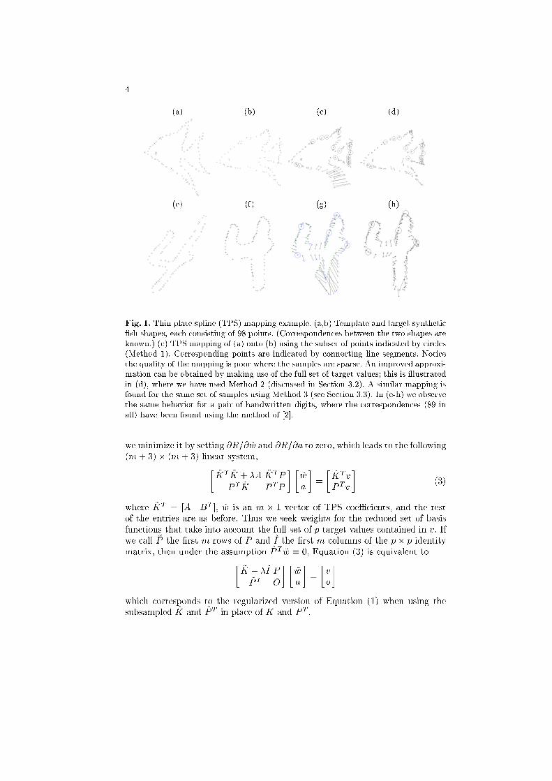
Fig. 1. Thin plate spline (TPS) mapping example. (a,b) Template and target synthetic

�sh shapes, each consisting of 98 points. (Correspondences between the two shapes are

known.) (c) TPS mapping of (a) onto (b) using the subset of points indicated by circles

(Method 1). Corresponding points are indicated by connecting line segments. Notice

the quality of the mapping is poor where the samples are sparse. An improved approxi-

mation can be obtained by making use of the full set of target values; this is illustrated

in (d), where we have used Method 2 (discussed in Section 3.2). A similar mapping is

found for the same set of samples using Method 3 (see Section 3.3). In (e-h) we observe

the same behavior for a pair of handwritten digits, where the correspondences (89 in

all) have been found using the method of [2].

we minimize it by setting @R=@ ~w and @R=@a to zero, which leads to the following(m+ 3)� (m+ 3) linear system,

�~KT ~K + �A ~KT

P

PT ~K P

TP

� �~wa

�=

�~KT

v

PTv

�(3)

where ~KT = [A BT ], ~w is an m � 1 vector of TPS coeÆcients, and the rest

of the entries are as before. Thus we seek weights for the reduced set of basisfunctions that take into account the full set of p target values contained in v. Ifwe call ~P the �rst m rows of P and ~I the �rst m columns of the p� p identitymatrix, then under the assumption ~P T ~w = 0, Equation (3) is equivalent to

�~K + �~I P~P T

O

� �~wa

�=

�v

o

�

which corresponds to the regularized version of Equation (1) when using thesubsampled ~K and ~P T in place of K and P T .

5

The application of this technique to the �sh and digit shapes is shown inFigure 1(d,h).

3.3 Method 3: Matrix Approximation

The essence of Method 2 was to use a subset of exact basis functions to approx-imate a full set of target values. We now consider an approach that uses a fullset of approximate basis functions to approximate the full set of target values.The approach is based on a technique known as the Nystr�om method.

The Nystr�om method provides a means of approximating the eigenvectorsof K without using C. It was originally developed in the late 1920s for thenumerical solution of eigenfunction problems [1] and was recently used in [11]for fast approximate Gaussian process regression and in [8] (implicitly) to speedup several machine learning techniques using Gaussian kernels. Implicit to theNystr�om method is the assumption that C can be approximated by BT

A�1B,

i.e.

K =

�A B

BTBTA�1B

�(4)

If rank(K) = m and the m rows of the submatrix [A B] are linearly indepen-dent, then K = K. In general, the quality of the approximation can be expressedas the norm of the di�erence C �B

TA�1B, the Schur complement of K.

Given the m � m diagonalization A = U�UT , we can proceed to �nd the

approximate eigenvectors of K:

K = ~U� ~UT; with ~U =

�U

BTU�

�1

�(5)

Note that in general the columns of ~U are not orthogonal. To address this, �rstde�ne Z = ~U�1=2 so that K = ZZ

T . Let Q�QT denote the diagonalizationof ZT

Z. Then the matrix V = ZQ��1=2 contains the leading orthonormalized

eigenvectors of K, i.e. K = V �VT , with V T

V = I .

From the standard formula for the partitioned inverse of L, we have

L�1 =

�K�1 +K

�1PS

�1PTK�1 �K�1

PS�1

�S�1P TK�1

S�1

�; S = �P T

K�1P

and thus �w

a

�= L

�1

�v

o

�=

�(I +K

�1PS

�1PT )K�1

v

�S�1P TK�1v

�

Using the Nystr�om approximation to K, we have K�1 = V ��1VT and

w = (I + V ��1VTP S

�1PT )V ��1

VTv ;

a = �S�1P TV �

�1VTv

6

(a) (b) (c)

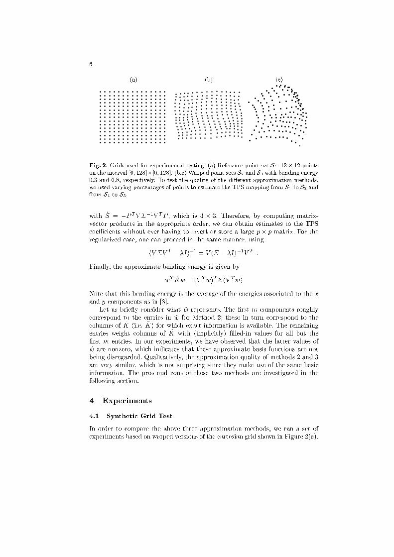
Fig. 2. Grids used for experimental testing. (a) Reference point set S1: 12� 12 points

on the interval [0; 128]�[0; 128]. (b,c) Warped point sets S2 and S3 with bending energy

0:3 and 0:8, respectively. To test the quality of the di�erent approximation methods,

we used varying percentages of points to estimate the TPS mapping from S1 to S2 and

from S1 to S3.

with S = �P TV �

�1VTP , which is 3 � 3. Therefore, by computing matrix-

vector products in the appropriate order, we can obtain estimates to the TPScoeÆcients without ever having to invert or store a large p� p matrix. For theregularized case, one can proceed in the same manner, using

(V �V T + �I)�1 = V (� + �I)�1V T:

Finally, the approximate bending energy is given by

wTKw = (V T

w)T�(V Tw)

Note that this bending energy is the average of the energies associated to the xand y components as in [3].

Let us brie y consider what w represents. The �rst m components roughlycorrespond to the entries in ~w for Method 2; these in turn correspond to thecolumns of K (i.e. ~K) for which exact information is available. The remainingentries weight columns of K with (implicitly) �lled-in values for all but the�rst m entries. In our experiments, we have observed that the latter values ofw are nonzero, which indicates that these approximate basis functions are notbeing disregarded. Qualitatively, the approximation quality of methods 2 and 3are very similar, which is not surprising since they make use of the same basicinformation. The pros and cons of these two methods are investigated in thefollowing section.

4 Experiments

4.1 Synthetic Grid Test

In order to compare the above three approximation methods, we ran a set ofexperiments based on warped versions of the cartesian grid shown in Figure 2(a).

7

5 10 15 20 25 300

1

2

3

4

5

6

7

8

Percentage of samples used

MS

E

If=0.3

Method 1Method 2Method 3

5 10 15 20 25 300

1

2

3

4

5

6

7

8

Percentage of samples used

MS

E

If=0.8

Method 1Method 2Method 3

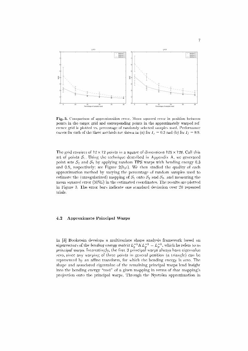
Fig. 3. Comparison of approximation error. Mean squared error in position between

points in the target grid and corresponding points in the approximately warped ref-

erence grid is plotted vs. percentage of randomly selected samples used. Performance

curves for each of the three methods are shown in (a) for If = 0:3 and (b) for If = 0:8.

The grid consists of 12�12 points in a square of dimensions 128�128. Call thisset of points S1. Using the technique described in Appendix A, we generatedpoint sets S2 and S3 by applying random TPS warps with bending energy 0:3and 0:8, respectively; see Figure 2(b,c). We then studied the quality of eachapproximation method by varying the percentage of random samples used toestimate the (unregularized) mapping of S1 onto S2 and S3, and measuring themean squared error (MSE) in the estimated coordinates. The results are plottedin Figure 3. The error bars indicate one standard deviation over 20 repeatedtrials.

4.2 Approximate Principal Warps

In [3] Bookstein develops a multivariate shape analysis framework based oneigenvectors of the bending energy matrix L�1p KL

�1

p = L�1

p , which he refers to asprincipal warps. Interestingly, the �rst 3 principal warps always have eigenvaluezero, since any warping of three points in general position (a triangle) can berepresented by an aÆne transform, for which the bending energy is zero. Theshape and associated eigenvalue of the remaining principal warps lend insightinto the bending energy \cost" of a given mapping in terms of that mapping'sprojection onto the principal warps. Through the Nystr�om approximation in

8

Method 3, one can produce approximate principal warps using L�1p as follows:

L�1

p = K�1 + K

�1PS

�1PTK�1

= V ��1VT + V �

�1VTPS

�1PTV �

�1VT

= V (��1 +��1VTPS

�1PTV �

�1)V T

�= V �V

T

where�

�= �

�1 +��1VTPS

�1PTV �

�1 =WDWT

to obtain orthogonal eigenvectors we proceed as in section 3.3 to get

� = W �WT

where W�=WD

1=2Q�

1=2 and Q�QT is the diagonalization of D1=2W

TWD

1=2.Thus we can write

L�1

p = V W �WTVT

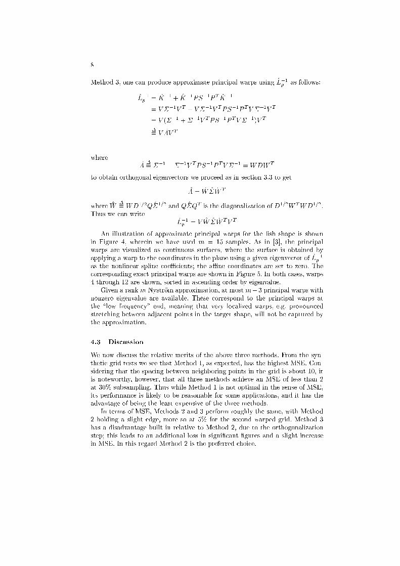
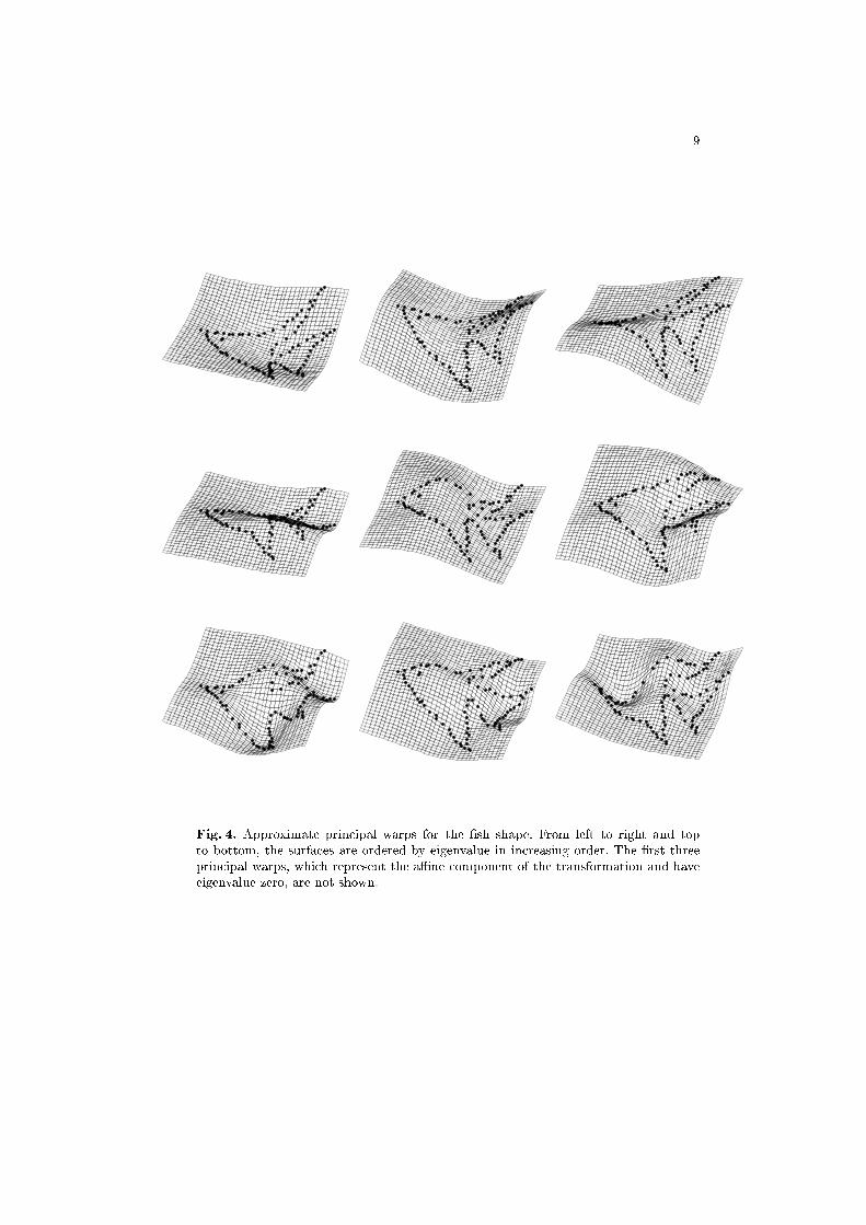
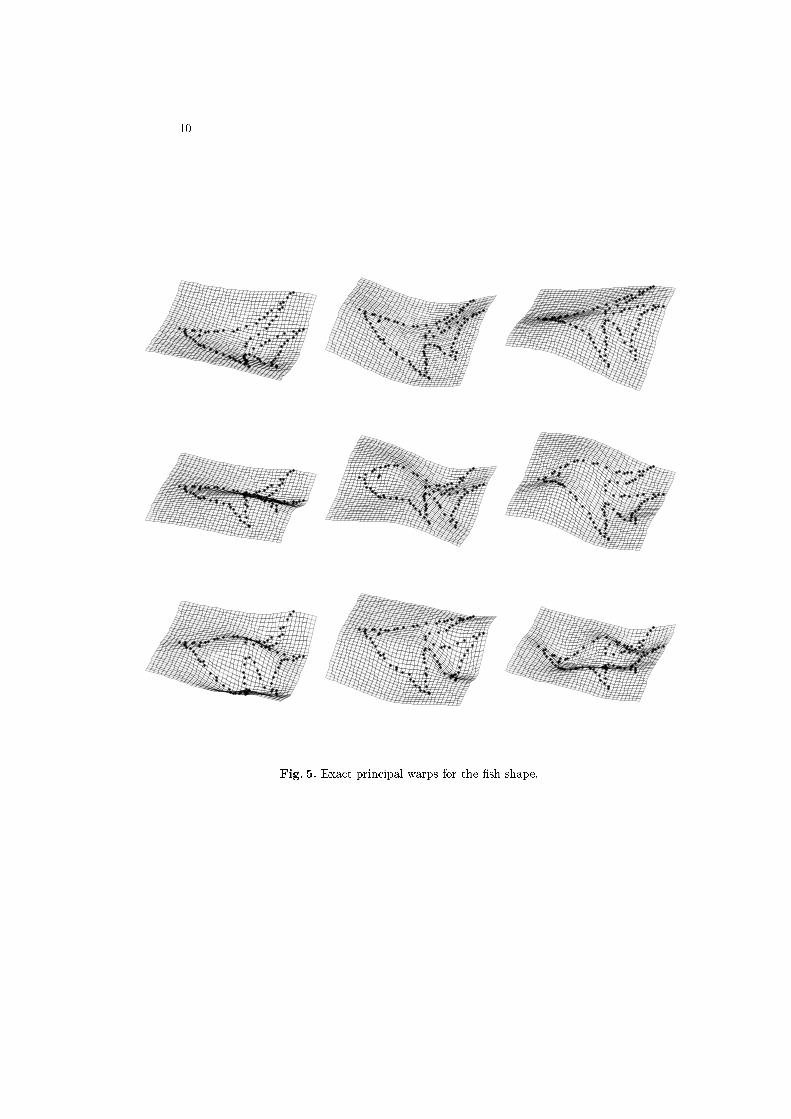
An illustration of approximate principal warps for the �sh shape is shownin Figure 4, wherein we have used m = 15 samples. As in [3], the principalwarps are visualized as continuous surfaces, where the surface is obtained byapplying a warp to the coordinates in the plane using a given eigenvector of L�1pas the nonlinear spline coeÆcients; the aÆne coordinates are set to zero. Thecorresponding exact principal warps are shown in Figure 5. In both cases, warps4 through 12 are shown, sorted in ascending order by eigenvalue.

Given a rank m Nystr�om approximation, at most m�3 principal warps withnonzero eigenvalue are available. These correspond to the principal warps atthe \low frequency" end, meaning that very localized warps, e.g. pronouncedstretching between adjacent points in the target shape, will not be captured bythe approximation.

4.3 Discussion

We now discuss the relative merits of the above three methods. From the syn-thetic grid tests we see that Method 1, as expected, has the highest MSE. Con-sidering that the spacing between neighboring points in the grid is about 10, itis noteworthy, however, that all three methods achieve an MSE of less than 2at 30% subsampling. Thus while Method 1 is not optimal in the sense of MSE,its performance is likely to be reasonable for some applications, and it has theadvantage of being the least expensive of the three methods.

In terms of MSE, Methods 2 and 3 perform roughly the same, with Method2 holding a slight edge, more so at 5% for the second warped grid. Method 3has a disadvantage built in relative to Method 2, due to the orthogonalizationstep; this leads to an additional loss in signi�cant �gures and a slight increasein MSE. In this regard Method 2 is the preferred choice.

9

Fig. 4. Approximate principal warps for the �sh shape. From left to right and top

to bottom, the surfaces are ordered by eigenvalue in increasing order. The �rst three

principal warps, which represent the aÆne component of the transformation and have

eigenvalue zero, are not shown.

10

Fig. 5. Exact principal warps for the �sh shape.

11

(a) (b)

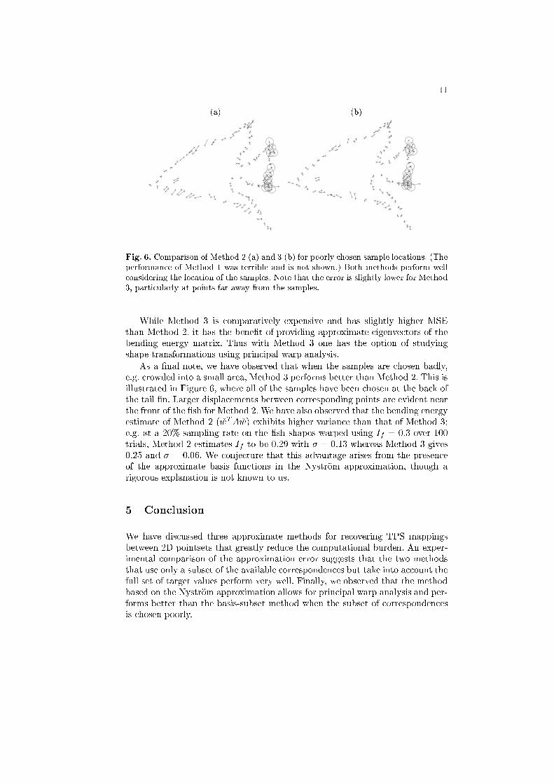
Fig. 6. Comparison of Method 2 (a) and 3 (b) for poorly chosen sample locations. (The

performance of Method 1 was terrible and is not shown.) Both methods perform well

considering the location of the samples. Note that the error is slightly lower for Method

3, particularly at points far away from the samples.

While Method 3 is comparatively expensive and has slightly higher MSEthan Method 2, it has the bene�t of providing approximate eigenvectors of thebending energy matrix. Thus with Method 3 one has the option of studyingshape transformations using principal warp analysis.

As a �nal note, we have observed that when the samples are chosen badly,e.g. crowded into a small area, Method 3 performs better than Method 2. This isillustrated in Figure 6, where all of the samples have been chosen at the back ofthe tail �n. Larger displacements between corresponding points are evident nearthe front of the �sh for Method 2. We have also observed that the bending energyestimate of Method 2 ( ~wT

A ~w) exhibits higher variance than that of Method 3;e.g. at a 20% sampling rate on the �sh shapes warped using If = 0:3 over 100trials, Method 2 estimates If to be 0:29 with � = 0:13 whereas Method 3 gives0:25 and � = 0:06. We conjecture that this advantage arises from the presenceof the approximate basis functions in the Nystr�om approximation, though arigorous explanation is not known to us.

5 Conclusion

We have discussed three approximate methods for recovering TPS mappingsbetween 2D pointsets that greatly reduce the computational burden. An exper-imental comparison of the approximation error suggests that the two methodsthat use only a subset of the available correspondences but take into account thefull set of target values perform very well. Finally, we observed that the methodbased on the Nystr�om approximation allows for principal warp analysis and per-forms better than the basis-subset method when the subset of correspondencesis chosen poorly.

12

Acknowledgments The authors wish to thanks Charless Fowlkes, Jitendra Malik,Andrew Ng, Lorenzo Torresani, Yair Weiss, and Alice Zheng for helpful discus-sions. We would also like to thank Haili Chui and Anand Rangarajan for usefulinsights and for providing the �sh datasets.

Appendix: Generating Random TPS Transformations

To produce a random TPS transformation with bending energy �, �rst choose aset of p reference points (e.g. on a grid) and form L

�1

p . Now generate a randomvector u, set its last three components to zero, and normalize it. Compute thediagonalization L�1p = U�U

T , with the eigenvalues sorted in descending order.

Finally, compute w =p�U�

1=2u. Since If is una�ected by the aÆne terms,

their values are arbitrary; we set translation to (0; 0) and scaling to (1; 0) and(0; 1).

References

1. C. T. H. Baker. The numerical treatment of integral equations. Oxford: Clarendon

Press, 1977.

2. S. Belongie, J. Malik, and J. Puzicha. Matching shapes. In Proc. 8th Int'l. Conf.

Computer Vision, volume 1, pages 454{461, July 2001.

3. F. L. Bookstein. Principal warps: thin-plate splines and decomposition of defor-

mations. IEEE Trans. Pattern Analysis and Machine Intelligence, 11(6):567{585,

June 1989.

4. H. Chui and A. Rangarajan. A new algorithm for non-rigid point matching. In

Proc. IEEE Conf. Comput. Vision and Pattern Recognition, pages 44{51, June

2000.

5. M.H. Davis, A. Khotanzad, D. Flamig, and S. Harms. A physics-based coordinate

transformation for 3-d image matching. IEEE Trans. Medical Imaging, 16(3):317{

328, June 1997.

6. F. Girosi, M. Jones, and T. Poggio. Regularization theory and neural networks

architectures. Neural Computation, 7(2):219{269, 1995.

7. M. J. D. Powell. A thin plate spline method for mapping curves into curves in two

dimensions. In Computational Techniques and Applications (CTAC95), Melbourne,

Australia, 1995.

8. A.J. Smola and B. Sch�olkopf. Sparse greedy matrix approximation for machine

learning. In ICML, 2000.

9. G. Wahba. Spline Models for Observational Data. SIAM, 1990.

10. Y. Weiss. Smoothness in layers: Motion segmentation using nonparametric mixture

estimation. In Proc. IEEE Conf. Comput. Vision and Pattern Recognition, pages

520{526, 1997.

11. C. Williams and M. Seeger. Using the Nystr�om method to speed up kernel ma-

chines. In T. K. Leen, T. G. Dietterich, and V. Tresp, editors, Advances in Neural

Information Processing Systems 13: Proceedings of the 2000 Conference, pages

682{688, 2001.