THE FREE-FALL DETERMINATION OF THE

UNIVERSAL CONSTANT OF GRAVITY

by

JOSHUA PETER SCHWARZ

B. A., University of Massachusetts,1993

M. S., University of Colorado, 1996

A thesis submitted to the

Faculty of the Graduate School of the

University of Colorado in partial ful�llment

of the requirements for the degree of

Doctor of Philosophy

Department of Physics

1998

This thesis entitled:The Free-Fall Determination of the Universal Constant of Gravity

written by Joshua Peter Schwarzhas been approved for the Department of Physics

James Faller

Douglas Robertson

David Bartlett

John Hall

Date

The �nal copy of this thesis has been examined by the signatories, and we �ndthat both the content and the form meet acceptable presentation standards of

scholarly work in the above mentioned discipline.

iii

Schwarz, Joshua Peter (Ph. D.,Physics)

The Free-Fall Determination of the Universal Constant of Gravity

Thesis directed by Professor Adjoint James Faller

The Newtonian constant of gravity, G, is the constant of proportionality

that scales the magnitude of the gravitational force between masses. G is the least

precisely known of all fundamental constants. Recent high-precision experiments

to measure G have produced highly discordant results, with values spread over a

range of 0.7%. The situation is almost incredible; the second digit of the value is

in contention and experiments disagree by as much as 50 of their individual error

estimates.

We have developed a new determination that uses an absolute free-fall

gravimeter to sense the gravitational attraction between a known source mass

and a falling test mass. We use a one-half metric ton source mass whose posi-

tion is alternated from above to below the dropping region, either decreasing or

increasing the observed acceleration of the test mass. The source mass generates

a di�erential signal of 8 parts in 107 of the local acceleration due to the Earth.

This method is independent of many of the systematic errors associated with the

traditional torsion balance experiments upon which the accepted value of G is

based.

Using this \free-fall" method in two data runs of approximately two weeks,

we have found a value of G at the level of 1100 ppm. Our value is: G = (6.6873 �0.0076) X10�11 m3/kg-s2. This value lies in the approximate center of the range

of recent results

ACKNOWLEDGEMENTS

Many people have o�ered assistance with my experiment. Tim Niebauer

originally suggested the method of using the gravimeter to measure the acceler-

ation signal of a source mass to determine G. But there is no doubt in my mind

that the person most responsible for the free fall experiment was Jim Faller. Jim

provided the energy and drive to get the experiment ying, and in many respects

drew me along for the ride. His was the insight that lead to our source mass

design, and also provided an example of the type of thought that I most enjoy

attempting.

Doug Robertson was like a second advisor to me. While Jim discussed (and

argued) di�erent points of apparatus with me, Doug and I worked closely on the

software framework that was crucial for the experiment. Doug o�ered liberal

constructive criticism on my rough drafts, and good ideas about the experiment.

In more practical ways the instrument makers John Andru, Dave Alchen-

berger, Jim Csotty, Blaine Horner, Cole Briggs, Seth Wieman, Hans Rohner, and

(especially!) Hans Green helped me (or did I help them?) with the design of the

lifting assembly. I certainly was no help to Hans Green or Blaine when they did

the actual work.

I didn't understand the purpose of the supply o�ce until it was too late.

That didn't stop Ed Holliness, Maryly Dole, Brian Lynch and David Tegart from

defying all the laws of physics I learned about to get me everything I desperately

v

needed (UPS RED!) on time. Ed and Brian also helped me work on my ping pong

game and throwing arm. In this capacity they boosted my self con�dence to the

heights required to submit a dissertation.

The last two paragraphs have mentioned many people, yet it only covers

the �rst oor of JILA. The Computing and Electronics Department is on the

second oor. Terry Brown, Joel Frahm, Alan Dunwell, James Fung-A-Fat, Paul

Beckingham, Mike Whitmore, Ralph Mitchell, Nick Metro, Peter Ruprecht, and

Chela Kunasz have helped me with all my electronics and computer needs. Terry

Brown, especially, worked hard to �ll my electronics-empty skull with ideas about

the discriminator circuit of the gravimeter (Chapter 3). He also helped me with

my arm, and kindly ran patterns for a rookie QB. James kept me honest by toying

with me on the raquetball court. He would have ruined my self con�dence, if I

had been so foolish as to challenge him while working on this thesis.

The Scienti�c Reports O�ce is also on the second oor. It's in a corner in

the building, where the Jewels are kept. Laurie Kovalenko and Marilee DeGoede

waded through so many sentences like this one that I can't help su�ering from

feelings of deep remorse | although I also experience feelings of thanks and

admiration because they were both such good writers, knowledgeable like I am

not, and feelings of regret because I'm leaving and won't be able to depend on

their help again, never ever, ever any more | maybe.

Outside of JILA the kind folks at Micro-g Solutions, Inc. were a great help

to us. They worked hard to help us get the experiment up and running quickly

so that we could capitalize on the gravimeter time were allocated. Tim Niebauer,

Fred Klopping, Kip Buxton, Jess Valentine, Jerry Gschwind and Echo never let

us down. I'd especially like to thank Fred and Jess, who were always very nice to

me even though I was needy.

From NOAA and the Table Mountain Gravity Observatory J.D. Williams,

vi

Tonie van Dam, Dan Winister and Glenn Sasagawa helped us wade through red

tape on our way to borrowing the gravimeters we used.

I've thanked the people who have helped with the experiment, and now

I'd like to give a hearty handshake1 to all the people who have helped me to

make it through | not by pointing out systematic errors in our experiment, or by

suggesting alternate data analysis techniques, but by helping with \the life part".

Many people I've already mentioned fall into this class. Jim Faller, for example,

supported my interests in subjects apart from physics. We had many enjoyable

conversations about Music, Sport, and Fine Dining that helped me keep proper

perspective. Every one in the instrument shop, too, always made me feel welcome

to shoot the breeze, have some popcorn and join up for a ride up Flagsta�.

Lisa Perry, LaReina Romero, Cheryl Glenn, Fran Haas, and even Leslie Haas

were almost always available for a quick chat whenever the mood arose. Cheryl

has su�ered through hummed melodies from my singing classes, while Lisa was

always quick to demonstrate proper technique (not just in singing).

Before there was JILA there was the Department of Physics, and classes.

Both Susan Thompson and Linda of \The Department" made me feel like more

than a cog in the machine. Somehow they also made sure that I ful�lled the

bureaucratic requirements of the grad school | two tough jobs.

Without Harold Volkie Parks, Darren Link, and Greg Rakness I never would

have scraped by. I needed three full-time tutors, and luckily that's what I got.

These three even helped feed me, by working out a system where I was taken to

lunch by everyone who got better exam scores than mine. Such generosity of time,

knowledge and food is too rare. Nevertheless I found similar generosity (well, two

of three. . . ) in all my classmates. I think that we were all lucky in our peers.

That leaves all the special people. I hope they know who they are.

1 I had \hug" here, but the �rst person I started to write about was Jim. . .

CONTENTS

CHAPTER

1 INTRODUCTION 1

1.1 G-Whiz: The Current Situation . . . . . . . . . . . . . . . . . . . 6

1.2 The Free-Fall Method . . . . . . . . . . . . . . . . . . . . . . . . . 10

2 THEORY 15

2.1 Mutual Attraction of the Free-Falling and Source Masses . . . . . 16

2.2 Theoretical Determination of the Trajectory . . . . . . . . . . . . 20

2.3 The Solutions . . . . . . . . . . . . . . . . . . . . . . . . . . . . . 22

3 EXPERIMENTAL APPARATUS 26

3.1 The Measurement System . . . . . . . . . . . . . . . . . . . . . . 26

3.1.1 The Dropping System . . . . . . . . . . . . . . . . . . . . 27

3.1.2 The Interferometer System . . . . . . . . . . . . . . . . . . 31

3.1.3 The FABIO system . . . . . . . . . . . . . . . . . . . . . . 33

3.1.4 Phase Shifts at the Discriminator Input . . . . . . . . . . . 34

3.1.5 The Position Reference System . . . . . . . . . . . . . . . 36

3.2 The Source Mass . . . . . . . . . . . . . . . . . . . . . . . . . . . 38

3.2.1 The Tungsten Masses . . . . . . . . . . . . . . . . . . . . . 43

3.2.2 The Drive/Support Structure . . . . . . . . . . . . . . . . 44

3.3 Superconducting Relative Gravimeter . . . . . . . . . . . . . . . . 47

viii

4 ANALYSIS 51

4.1 A Big Least Squares Solution . . . . . . . . . . . . . . . . . . . . 51

4.2 The Method of Parallels . . . . . . . . . . . . . . . . . . . . . . . 54

4.2.1 Di�erencing Techniques . . . . . . . . . . . . . . . . . . . 55

4.3 Dependence of �go on First Fringe Fit . . . . . . . . . . . . . . . . 57

5 ERROR ANALYSIS 62

5.1 General Error Analysis . . . . . . . . . . . . . . . . . . . . . . . . 62

5.1.1 Common mode errors . . . . . . . . . . . . . . . . . . . . . 62

5.1.2 Positioning Errors . . . . . . . . . . . . . . . . . . . . . . . 64

5.1.3 Modeling Errors . . . . . . . . . . . . . . . . . . . . . . . . 67

5.1.4 Numerical Techniques . . . . . . . . . . . . . . . . . . . . 68

5.1.5 Spurious Signals . . . . . . . . . . . . . . . . . . . . . . . . 69

5.1.6 Contaminated Data . . . . . . . . . . . . . . . . . . . . . . 69

5.2 Sources of Systematic Error . . . . . . . . . . . . . . . . . . . . . 70

5.2.1 Air Gap Modulation . . . . . . . . . . . . . . . . . . . . . 73

5.2.2 Thermal Signals . . . . . . . . . . . . . . . . . . . . . . . . 82

5.2.3 Systematic Laser Excitation . . . . . . . . . . . . . . . . . 88

5.2.4 Laser Verticality and Floor Tilts . . . . . . . . . . . . . . . 88

5.2.5 Ball Wear . . . . . . . . . . . . . . . . . . . . . . . . . . . 91

5.2.6 Phase Coherent Excitation of the Super Spring . . . . . . 92

5.2.7 Magnetic E�ects - Static Fields . . . . . . . . . . . . . . . 94

5.2.8 Magnetic E�ects { Dynamic Fields . . . . . . . . . . . . . 96

5.2.9 Contaminated Fringes . . . . . . . . . . . . . . . . . . . . 101

5.2.10 Unquanti�ed Error Sources . . . . . . . . . . . . . . . . . 104

5.3 Evidence of other Systematic Errors . . . . . . . . . . . . . . . . . 108

5.3.1 Residual Analysis . . . . . . . . . . . . . . . . . . . . . . . 110

ix

6 DATA AND RESULTS 113

6.1 Data Runs . . . . . . . . . . . . . . . . . . . . . . . . . . . . . . . 113

6.1.1 The Bronze Mass Experiment . . . . . . . . . . . . . . . . 113

6.1.2 May 1997 Experiment . . . . . . . . . . . . . . . . . . . . 118

6.1.3 May 1998 Experiment . . . . . . . . . . . . . . . . . . . . 127

6.2 Combined Results . . . . . . . . . . . . . . . . . . . . . . . . . . . 132

7 CONCLUSION 136

7.1 Results . . . . . . . . . . . . . . . . . . . . . . . . . . . . . . . . . 137

7.2 Future . . . . . . . . . . . . . . . . . . . . . . . . . . . . . . . . . 138

BIBLIOGRAPHY 141

APPENDIX

AMASS METROLOGY 146

A.1 Metrology of the Source Mass . . . . . . . . . . . . . . . . . . . . 147

A.2 Modeling the Test Mass . . . . . . . . . . . . . . . . . . . . . . . 159

B ERROR CALCULATIONS 166

B.1 Positioning Errors . . . . . . . . . . . . . . . . . . . . . . . . . . . 166

B.1.1 Source Mass Positioning Errors . . . . . . . . . . . . . . . 166

B.1.2 Proof Mass Positioning errors . . . . . . . . . . . . . . . . 167

B.1.3 Extracted Positions . . . . . . . . . . . . . . . . . . . . . . 167

B.2 Spurious Signals . . . . . . . . . . . . . . . . . . . . . . . . . . . . 168

B.2.1 Di�erential Magnetic Forces. . . . . . . . . . . . . . . . . . 168

B.3 Modeling Errors . . . . . . . . . . . . . . . . . . . . . . . . . . . . 174

B.3.1 Source Mass Modeling Errors . . . . . . . . . . . . . . . . 174

x

B.3.2 Proof Mass Modeling errors . . . . . . . . . . . . . . . . . 177

B.4 Numerical System . . . . . . . . . . . . . . . . . . . . . . . . . . . 181

B.4.1 Absolute Accuracy of Quadrature: The Integration Over

the Source Mass . . . . . . . . . . . . . . . . . . . . . . . . 181

B.4.2 Assumption of Cylindrical Symmetry . . . . . . . . . . . . 183

B.4.3 Di�erential Precision of the System . . . . . . . . . . . . . 185

FIGURES

Figure

1.1 Schematic of a torsion balance . . . . . . . . . . . . . . . . . . . . 4

1.2 Schematic of the time-of-swing method. . . . . . . . . . . . . . . . 5

1.3 Recent G results . . . . . . . . . . . . . . . . . . . . . . . . . . . 7

1.4 Schematic of the experimental apparatus . . . . . . . . . . . . . . 13

1.5 Photograph of the experimental apparatus . . . . . . . . . . . . . 14

2.1 Acceleration �eld of the source mass . . . . . . . . . . . . . . . . 24

2.2 Perturbation to the free-fall solution. . . . . . . . . . . . . . . . . 25

3.1 Schematic of the dropping chamber . . . . . . . . . . . . . . . . . 28

3.2 Interferometer schematic. . . . . . . . . . . . . . . . . . . . . . . . 32

3.3 Schematic of the super spring . . . . . . . . . . . . . . . . . . . . 37

3.4 Schematic of the source mass . . . . . . . . . . . . . . . . . . . . 41

3.5 Photo of the source mass . . . . . . . . . . . . . . . . . . . . . . . 42

3.6 View of pivot-balance system . . . . . . . . . . . . . . . . . . . . 45

3.7 Photo of screw drive . . . . . . . . . . . . . . . . . . . . . . . . . 47

3.8 Schematic of superconducting relative gravimeter . . . . . . . . . 49

4.1 Di�erencing methods . . . . . . . . . . . . . . . . . . . . . . . . . 56

4.2 Quality of �t for position of source mass . . . . . . . . . . . . . . 58

4.3 Comparison of di�erent SOD results . . . . . . . . . . . . . . . . 60

xii

4.4 Extracted values of the start-of-drop position . . . . . . . . . . . . 61

5.1 Change of proof mass acceleration with radial position . . . . . . 66

5.2 Commentary on data exclusion . . . . . . . . . . . . . . . . . . . 71

5.3 Vertical motion of the airgap . . . . . . . . . . . . . . . . . . . . . 74

5.4 Amplitude spectrum of the airgap motion . . . . . . . . . . . . . 75

5.5 Comparison of airgap theory to measurement . . . . . . . . . . . 77

5.6 Weighted motion of airgap interface . . . . . . . . . . . . . . . . . 79

5.7 Scaling of airgap theory to measurement . . . . . . . . . . . . . . 81

5.8 Comparison of airgap motion with source mass in upper or lower

position . . . . . . . . . . . . . . . . . . . . . . . . . . . . . . . . 83

5.9 Temperature signal in a test for heating errors . . . . . . . . . . . 85

5.10 Time-binned di�erences from the 1998 experiment . . . . . . . . . 87

5.11 Residuals corrected for laser-bauble signal . . . . . . . . . . . . . 89

5.12 Pointwise-averaged sets, 1997 and 1998 data runs . . . . . . . . . 94

5.13 Setup to measure AC magnetic forces . . . . . . . . . . . . . . . . 100

5.14 Plot of data with missed fringes . . . . . . . . . . . . . . . . . . . 102

5.15 A test for corrupt data: variation of g with �rst �t fringe . . . . . 104

5.16 Plot of suspicious data, set averaged . . . . . . . . . . . . . . . . 107

5.17 Di�erence signal: theory and measurement . . . . . . . . . . . . . 109

5.18 Residuals-to-drop averaged over 150,000 drops . . . . . . . . . . . 111

6.1 Photo of bronze mass experiment . . . . . . . . . . . . . . . . . . 115

6.2 Bronze mass experiment, data sample . . . . . . . . . . . . . . . . 117

6.3 Bronze mass experiment, results . . . . . . . . . . . . . . . . . . . 117

6.4 May, 1997 experiment. Individual di�erences . . . . . . . . . . . . 120

6.5 May, 1997 experiment, results . . . . . . . . . . . . . . . . . . . . 121

6.6 May, 1997 experiment. Power spectral analysis. . . . . . . . . . . 122

xiii

6.7 1997 experiment, G as a function of �rst �t fringe . . . . . . . . . 124

6.8 1997 experiment, Uncertainty in G related to G values . . . . . . 125

6.9 Daily results of the 1998 experiment . . . . . . . . . . . . . . . . 129

6.10 Individual di�erences from the 1998 experiment . . . . . . . . . . 130

6.11 Power spectral analysis of 1998 data. . . . . . . . . . . . . . . . . 131

6.12 1998 experiment, G as function of �rst fringe �t . . . . . . . . . . 133

6.13 Final results of the Free Fall experiment . . . . . . . . . . . . . . 135

A.1 Cylinder arrangement in source mass . . . . . . . . . . . . . . . . 152

A.2 Photograph of the proof mass. . . . . . . . . . . . . . . . . . . . . 164

A.3 Drawing of the proof mass model. . . . . . . . . . . . . . . . . . . 165

B.1 Vertical magnetic �eld and gradient, theory . . . . . . . . . . . . 169

B.2 Study of error introduced by proof mass model vertical granularity 178

B.3 Study of error introduced by proof mass model radial granularity 179

B.4 Study of error arising from vertical interpolation grid density . . . 182

B.5 Study of error arising from vertical interpolation grid density on

the radial dimension . . . . . . . . . . . . . . . . . . . . . . . . . 183

B.6 Study of error arising from radial interpolation grid density . . . . 184

B.7 Study of error arising from radial interpolation grid density . . . . 184

B.8 Vertical acceleration �eld with the assumption of cylindrically sym-

metric source mass . . . . . . . . . . . . . . . . . . . . . . . . . . 186

B.9 Errors arising from assumption of cylindrical source mass symmetry 186

TABLES

Table

5.1 Summary of major error sources. . . . . . . . . . . . . . . . . . . 72

6.1 Main moments of the 1998 experiment distribution . . . . . . . . 128

A.1 Characteristics of the tungsten cylinders . . . . . . . . . . . . . . 150

A.2 Density variations in the tungsten cylinders . . . . . . . . . . . . 150

A.3 Model of the lower support plate, 1997 experiment . . . . . . . . . 154

A.4 Model of the upper plate, 1997 experiment . . . . . . . . . . . . . 155

A.5 Main model of the source mass, 1997 experiment . . . . . . . . . . 156

A.6 Model of the support plates, 1998 experiment . . . . . . . . . . . 157

A.7 Main model of the 1998 experiment . . . . . . . . . . . . . . . . . 158

A.8 Model of the Top Hat cap of the proof mass. All dimensions (po-

sition, height, rinner, routter, o�set) are in centimeters. The masses

are in grams. . . . . . . . . . . . . . . . . . . . . . . . . . . . . . 160

A.9 Model of proof mass: Tungsten balls, glass sphere, top hat cap. All

dimensions (position, height, rinner, routter, o�set) are in centime-

ters. The masses are in grams. . . . . . . . . . . . . . . . . . . . . 160

A.10 Model of proof mass: Corner cube holder and counter weight. All

dimensions (position, height, rinner, routter, o�set) are in centime-

ters. The masses are in grams. . . . . . . . . . . . . . . . . . . . . 161

xv

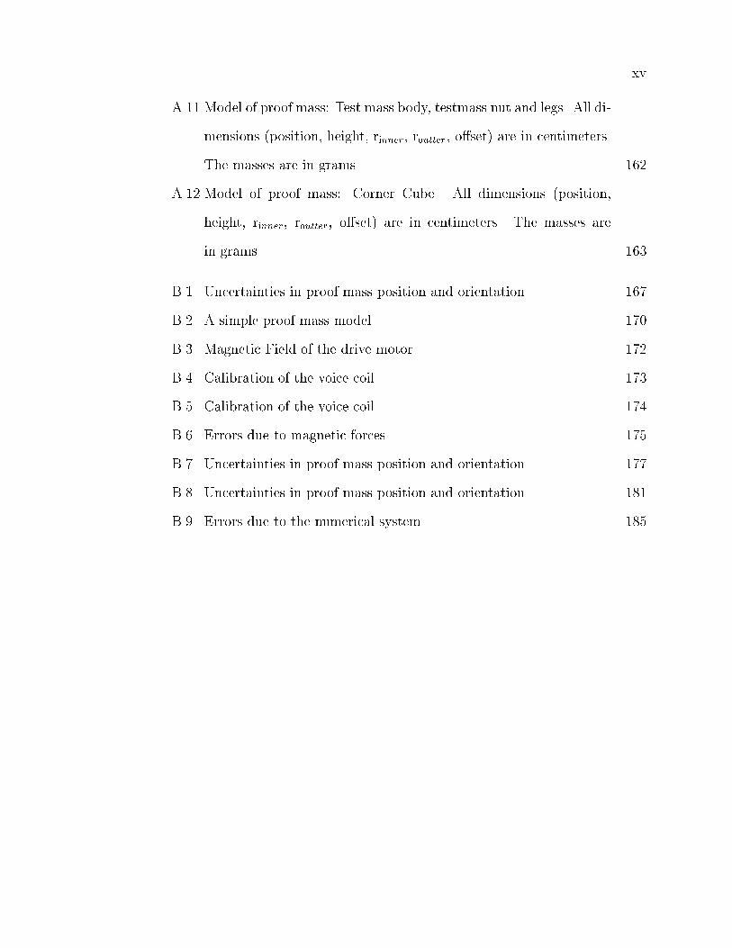
A.11 Model of proof mass: Test mass body, testmass nut and legs. All di-

mensions (position, height, rinner, routter, o�set) are in centimeters.

The masses are in grams. . . . . . . . . . . . . . . . . . . . . . . . 162

A.12 Model of proof mass: Corner Cube. All dimensions (position,

height, rinner, routter, o�set) are in centimeters. The masses are

in grams. . . . . . . . . . . . . . . . . . . . . . . . . . . . . . . . 163

B.1 Uncertainties in proof mass position and orientation . . . . . . . . 167

B.2 A simple proof mass model . . . . . . . . . . . . . . . . . . . . . . 170

B.3 Magnetic Field of the drive motor. . . . . . . . . . . . . . . . . . 172

B.4 Calibration of the voice coil. . . . . . . . . . . . . . . . . . . . . . 173

B.5 Calibration of the voice coil. . . . . . . . . . . . . . . . . . . . . . 174

B.6 Errors due to magnetic forces . . . . . . . . . . . . . . . . . . . . 175

B.7 Uncertainties in proof mass position and orientation . . . . . . . . 177

B.8 Uncertainties in proof mass position and orientation . . . . . . . . 181

B.9 Errors due to the numerical system. . . . . . . . . . . . . . . . . . 185

CHAPTER 1

INTRODUCTION

The world we live in is largely de�ned by gravity. When we see the waves

of the ocean below or the sky above we are conscious of the e�ects of this far

reaching force. The atmosphere we breathe, the light of the sun, the fall of rain,

the shape of a ame | all are consequences of the attraction of matter.

For my ally is the Force. And a powerful ally it is. . . Its energysurrounds us and binds us. . . You must feel the Force around you.Here, between you. . . me. . . the tree. . . the rock. . . everywhere!Yes, even between this land and that ship!| Yoda, The Empire Strikes Back, George Lucas

The force that de�nes the arrangement of the stars above us is a subject

well deserving of appreciation, contemplation, and study. It is no wonder that for

thousands of years questions about gravity have occupied the minds of the curious

and contemplative.

Sir Isaac Newton provided the �rst model that we of the modern world cite

when considering the e�ects of this powerful attraction, in a description that all

physicists learn in the formative years of their studies:

F =GMm

r2

Just this snippet of information is very valuable, for it forms the basis of much

knowledge of how things interact { how the forces of gravity vary with mass and

distance.

2

Without the universal gravitational constant, G, it is not possible to scale

the force { to calculate the gravitational attractions between objects, even if their

masses and relative positions are known. Although the practical bene�ts of per-

forming this calculation are far and few between, the value of G is of real interest

in some areas of physical research. Geophysicists, geologists, and seismologists

use the value of G to deduce information about the structure and makeup of

the Earth. Cosmologists and astronomers, on the other hand, base information

concerning astronomical structure and the early universe on G[1]. Theorists who

work on uni�cation the four known forces need to know G to gauge the success of

their theories.

It is the search for this constant that forms the basis of this dissertation, and

has motivated many experiments since the late eighteenth century. Experiments

to measure G have all had to deal with the same set of tough issues. Most

important is the requirement that the experimental system be very sensitive to

the gravitational �eld of a well-known mass, yet simultaneously be very insensitive

to all other forces. This is a di�cult demand to meet because the force of gravity

is so weak in comparison to other forces. The following calculation illustrates this

point. The accepted value for G, as of 1998, was

G = (6:6726� 0:00085)� 10�11 m3=kg � s2 (1.1)

based on the 1986 adjustment of standards. We can use this value to estimate

the gravitational attraction between two average sized people (Jack and Jill) in a

close hug:

F =G � (MassJack)(MassJill)

Distance2

which may be approximately

F =(6:7X10�11m3=kg � s2)(65kg) � (50kg)

(0:3m)2= 2:4 � 10�7 N

3

This is equivalent to the weight of three tenths of one billionth of a gram (luckily

gravity is not the only attractive force!).

We don't generally think of gravity as weak because we associate it with the

pull of the entire Earth. Yet other forces can easily swamp gravity on many length

scales. An example is the electrostatic force; the minute charge picked up when

your feet scu� a rug is enough to cause slips of paper to stick to your hair, defying

the gravitational attraction of the whole world. A more quantitative comparison

can be made between the magnitude of the electric attraction of a proton for an

orbiting electron and the gravitational force between them. The electric force is

1040 times larger.

Another hard fact of G-measurements is that gravity can't be shielded. If I

wished to produce a region that was free of electric �elds, all I would have to do is

construct a conducting shell around the region. If I wanted to exclude magnetic

�elds, I could make the shell super conducting. If I need to exclude gravitational

�elds, then I had better think of a di�erent experiment!

For this reason G experiments are designed so that it is not necessary to

have a gravity-free environment for their success. Most experimenters, however,

would like to circumvent one major component of the gravity �eld that exists on

Earth { namely the attraction due to the planet itself. Experimentalists have

commonly attempted to do this by using a torsion �ber to support a dumbbell-

shaped beam. This allows horizontal forces to be expressed in twists of the �ber

support without strong dependence on the local acceleration.

Fibers have been most commonly used in torsion balances, �rst conceived by

the Minister John Price and used by Henry Cavendish in his famous determination

of G [2]. The torsion balance is used by measuring the shift of the equilibrium

position of the beam due to the gravitational attraction of external masses (Figure

1.1). Because �bers twist very easily even small gravitational forces produce a

4

. . .. . .

. . .. . .

. . .. . .

. .

. . .. . .

. . .. . .

. . .. . .

. .

Fiber

Beam

�

�

xx

xw

����

����

����

����

���

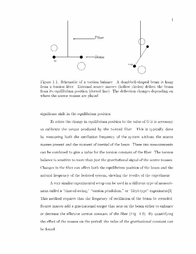
Figure 1.1: Schematic of a torsion balance. A dumbbell-shaped beam is hungfrom a torsion �ber. External source masses (hollow circles) de ect the beamfrom its equilibrium position (dotted line). The de ection changes depending onwhere the source masses are placed.

signi�cant shift in the equilibrium position.

To relate the change in equilibrium position to the value of G it is necessary

to calibrate the torque produced by the twisted �ber. This is typically done

by measuring both the oscillation frequency of the system without the source

masses present and the moment of inertial of the beam. These two measurements

can be combined to give a value for the torsion constant of the �ber. The torsion

balance is sensitive to more than just the gravitational signal of the source masses.

Changes in the �ber can a�ect both the equilibrium position of the beam and the

natural frequency of the isolated system, skewing the results of the experiment.

A very similar experimental setup can be used in a di�erent type of measure-

ment called a \time-of-swing," \torsion pendulum," or \Heyl-type" experiment[3].

This method requires that the frequency of oscillation of the beam be recorded.

Source masses add a gravitational torque that acts on the beam either to enhance

or decrease the e�ective torsion constant of the �ber (Fig. 1.2). By quantifying

the e�ect of the masses on the period, the value of the gravitational constant can

be found.

5

The vast majority of precision G experiments done since Cavendish have

used either torsion balances or torsion pendulums. Over the ninety years before

the 1986 setting of the accepted value, more than three quarters of all G mea-

surements used one of these two systems. Of the three most accurate experiments

before the reassesment of the accepted value in 1986, two (Luther and Towler

[4] and Sagitov et al.[5]) used torsion pendulums, while the third (Karagioz and

Izmailov ([6])) used a torsion balance. The accepted value of the constant, today,

is based on the Luther and Towler number. More complete discussion of the mea-

surement of G in the last 200 years may be found in Gillies[7], Bagley [8], and

Koldewyn [9].

A B

}} }}����

����

����

����

Figure 1.2: A schematic of the time-of-swing method. A torsion pendulum (in itsequilibrium position) is represented by the dumbbell-shaped rod. represents thetorsion support. The hollow circles represent source masses. A) The source massesgravitationally augment the restoring torque of the �ber, increasing the frequencyof oscillation. B) The source masses decrease the frequency of oscillation.

Recently �ber-based torsion experiments have come under attack. They

are subject to a systematic e�ect that was �rst recognized in 1995 by Kazuki

Kuroda[10]. The error arises because the anelastic relaxation e�ects in twisted

�bers change the torsion constant of the �bers; real �bers diverge slightly from

the simpler model of twisted members that had been used until Kuroda released

6

his �ndings. This systematic error a�ects both torsion balance and pendulum

experiments. Continuing research on this characteristic of �bers is ongoing [11, 12].

There are also plans to operate a torsion pendulum at cryogenic temperatures, to

reduce anelastic e�ects [13].

1.1 G-Whiz: The Current Situation

The dominance of torsion �ber based determinations of G, coupled with

uncertainty about �ber anelasticity, lead to four new experiments that have pro-

duced results in the last three years (Figure 1.3). The results vary over such a

large range (0.7%) that the probability that the disagreement is due to a statistical

uctuation is approximately one in 518.

The �rst measurement was conducted by Walech, Meyer, Piel and Schurr,

at the University of Wuppertal, Germany [18, 19]. The group used two simple

pendulums to support mirrors de�ning a microwave Fabry-P�erot resonator. By

placing a source mass system on the line between the pendulums, the distance be-

tween the two bobs was changed. The resonator measured the separation change,

thereby scaling G. Their initial result[18], released in 1995, was:

G = 6:6719� 0:0006 � 10�11m3=kg � s2

This value was the only recent result consistent with the accepted value. In 1998

large systematic errors associated with the positioning of their source masses came

to light. When they correct their previous result to re ect these errors, their value

changes to:

G = 6:6637� 0:0004� 0:0044 � 10�11 m3=kg � s2

This value lies 2 standard errors below the accepted value [16].

Fitzgerald and Armstrong of the New Zealand Standards used a nulled tor-

sion balance [15]. This is a normal torsion balance experiment with one important

7

6.65

6.66

6.67

6.68

6.69

6.7

6.71

6.72

6.73

Luther, Towler

New Zealand

WuppertalSwiss

PTB

Result

G X

1011

m3 /k

g−s

2

Figure 1.3: Four recent results of G experiments. The 1982 result of Luther andTowler at the NBS [4] is the basis of the accepted value. The results of the PTB(German Standards, 42� high [14]), the New Zealand Standards (10� low [15]),and a group at the University of Wuppertal (2� low [16]) were all released in 1995.A group in Switzerland released a preliminary result in 1998 (2� high [17])

8

di�erence | the torque of the source masses was not matched by the twist in the

�ber, but rather by a torque produced by electrostatic forcers. The forcers were

servoed to maintain the orientation of the beam. This method has the advantage

that the orientation of the beam doesn't change, so spatially variant horizontal

gravity gradients do not in uence the results. Also, this type of system is not

subject to �ber anelasticity problems. The major hurdle with this method is in

the calibration of the torque produced by the forcers. Fitzgerald and Armstrong

released a result in 1995:

G = 6:6656� 0:00063 � 10�11m3=kg � s2

This result is 11 standard errors ( about 0.1% ) below the accepted value.

At the Physikalisch-Technische Bundesanstalt (PTB)1 de Boer, Haars and

Michaelis have carried out a similar experiment for which planning began in 1976

[14, 20]. They used a compensated torsion balance with a mercury bearing, rather

than a �ber, to support the beam. This type of bearing is nearly free of static

friction. The experimenters made measurements of G at di�erent distances and

between di�erent materials. These measurements gave consistent results. In 1995

the �nal result of their measurement was released:

G = 6:7154� 0:00055 � 10�11m3=kg � s2

This represents a disagreement with the accepted value of more than 40 � (0.6%

high).

A group at the University of Z�urich, consisting of J. Schurr, F. Nolting and

W. K�undig [17, 21] is currently measuring the di�erence in the weight of two

masses2 . They modulate this di�erence by moving two source masses around the

1 The PTB is the German Bureau of Standards2 This method is similar, in some respects, to our own \free fall" method, and shares many

of its bene�ts. The di�erence, for example, is measured in the vertical direction, so this deter-mination is made with the perturbing gravitational attraction in-line with the attraction of theEarth.

9

two weights. The group uses two large asks containing 13.5 tons of mercury as

their source masses. They released a preliminary result (using water instead of

mercury in the asks) in February of 1998:

G = 6:6754� 0:0015 � 10�11m3=kg � s2

This result is 2� above the accepted value.

Let us summarize the situation. Many experiments have been e�ected re-

cently, yet at the level of a quarter percent there is no clear value for G. The new

experiments use a variety of methods, most moving away from twisted �ber ide-

ology, but their results fail to converge. The large spread in results compared to

small error estimates, as shown in Fig.1.3, indicates that there are large systematic

errors in at least two of the three high precision results.

A need for experiments that are independent of the torsion/twisted support

methodology exists. Consider that the two values with the largest discrepancies

with the accepted value are based on similar experiments using di�erent torsion

supports (PTB and New Zealand). Also recall that the great majority of G

experiments relied on a twisted �ber torsion approach to the measurement, a

method subject to systematic errors that are only now becoming understood.

The \Free Fall Measurement of G" is presented in this thesis. The free

fall measurement is unique in that it uses an unsupported test mass to sense the

gravitational force. It senses this force in a direction parallel to the acceleration

due to the Earth (no torque). This method, therefore, has a very di�erent set

of systematic errors than other G-experiments. We hope that our results will

add useful information in the current situation of nearly one-half a percent of

uncertainty in G.

10

1.2 The Free-Fall Method

The free-fall method depends on our ability to measure the amount that an

external source mass changes the acceleration of a freely falling object. First a

source mass is placed above the region in which the \test mass" falls. Here the

gravitational pull of the source mass acts in the opposite direction to the attraction

of the Earth, decreasing the downward acceleration of the test mass. Second

the source mass is placed below the drop region, where it augments the Earth's

attraction and the acceleration of the falling mass. If the change in acceleration

can be measured accurately, and if the geometry of the source and test masses are

well known, then we can determine G.

This is conceptually simple, yet in practice the subtleties of the measurement

are plentiful. These subtleties arise from the lack of an ideal mechanism to measure

the acceleration of the test mass. The acceleration signal produced by our source

mass is only 1 part in 107 of the signal of the Earth. Thus we need to precisely

measure a small acceleration signal on top of a huge o�set. To achieve an accuracy

in our measurement of 0.01%, we must have a precision of 1 part in 1011 in the

measurement of the absolute acceleration of the falling object. This is not an easy

task.

Fortunately free-fall gravimeters have been developed to precisely measure

the local acceleration of gravity, g. The gravimeter drops an object and records its

position as a function of time. By �tting the position/time curve with a parabola

the acceleration of the test mass is extracted.

Working at JILA we were perfectly poised to capitalize on the utility of

free-fall gravimeters for the G measurement. The gravimeter we used, a Micro-g

Solutions, Inc. model FG-5, grew out of free-fall gravimeter systems that were

developed in JILA by Jim Faller[22], James Hammond, Robert Rinker[23], Mark

11

Zumbergezumberge, and Tim Niebauer[24]. Tim originally suggested the idea for

the free-fall measurement of G, and is the head of the Micro-g Solutions, Inc.

Thus we had, at our elbows, a group of people with tremendous expertise with

the gravimeter system. Also the University of Colorado, which is associated with

JILA, owns an FG-5 that we were able to borrow for our measurements.

The experiment was carried out at the Table Mountain Gravity Observa-

tory (TMGO), a center for the research and development of absolute and rela-

tive gravimeters, 10 miles north of Boulder. TMGO is operated by the National

Oceanic and Atmospheric Administration (NOAA). Running the experiment at

TMGO was crucial to the success of the free-fall measurement because of the ex-

ceptional quality (low vibration noise) of the site. Also TMGO is equipped with

secondary measurement systems that were extremely helpful in our experiment.

A free fall gravimeter uses a laser interferometer system to track the mo-

tion of the falling test mass. The test mass contains a corner-cube retrore ector

that de�nes one arm of a Michaelson-type interferometer. Thus the interferometer

fringe crossings correspond to changes of the test mass's position. By incorporat-

ing a precise time standard, a stable position reference, and all the electronics and

hardware required to drop the test mass in vacuum, it is possible to record the

position as a function of time of the falling mass. The absolute accuracy of the

system is 1�Gal, or approximately one part in 109 of the acceleration due to the

Earth3 . It is limited by machine-dependent uncertainties arising from (among

other things) residual air pressure in the vacuum can, electrostatic forces, and the

attraction of the gravimeter itself.

In the free-fall G experiment we were more interested in the change of the

acceleration of the test mass than its absolute acceleration. This meant that we

were not limited by the accuracy of the gravimeter so much as by its precision. We

3 A Gal is a cm/s2, and a �Gal is 1e-6 Gal.

12

operated the gravimeter in a di�erential mode that eliminated \common mode"

errors in the measurement | errors that were independent of the source mass

position. This allowed us to achieve a precision in our result that is more than

twenty times greater than the absolute accuracy of the gravimeter.

The perturbing gravity �eld that changed the acceleration of the falling mass

was produced by a ring-shaped source mass made of 500 kg of tungsten alloy. The

use of a ring-shape gives a tremendous advantage over traditional spherical or solid

cylindrical source masses because the axial acceleration �eld produced by a ring

has two extrema. This means that there are two positions at which the �eld of

the masses doesn't change with a movement from that position; there are two

positions for the source mass that cause our results to be nearly insensitive to

positioning errors. The source mass was located alternately above and below the

drop zone in these two places, as shown in Fig.1.4. The actual experimental setup

is shown in Fig.1.5 with the source mass in its upper position.

Conceptually the experiment was a variant of a classical orbit determination

problem in which our free-falling test mass was the orbiting body [25]. In e�ect, we

did a satellite laser ranging experiment in a laboratory. But in contrast to classical

spacecraft tracking problems, where one determines the quantity GM (G times

the mass of the primary planet or star, M), we were able to extract G because

we measured M in the laboratory. The close analogy to conventional spacecraft

tracking problems allowed us to use a number of classical orbit determination

techniques.

13

Figure 1.4: A schematic cross-section of the experimental apparatus. The sourcemass was alternately placed at positions A and B at twenty minute (100 drop)intervals.

14

Figure 1.5: A photograph of the experimental apparatus. The source mass isin its upper optimal position around the dropping chamber. The interferometerlooks like a black box located below the dropping chamber. The super springhangs below the interferometer. The large aluminum structure was built for theG-experiment, and supported the source mass.

CHAPTER 2

THEORY

The underlying physics of the free-fall determination have been well under-

stood for hundreds of years. Two equations are su�cient to classically describe the

gravitational interaction between masses. Sir Isaac Newton �rst recognized the

relationship between the mass of two point particles (M and m), their separation

(d), and the magnitude of the gravitational force (F ) between them:

F =GmM

d2(2.1)

Newton's second law,

F = ma (2.2)

describes the acceleration, a, of a mass m, arising from the application of a vector

force, F. The second law, although only valid in a classical regime of low velocity,

is su�ciently accurate to describe the action of the free-fall experiment.

These equations allowed us to calculate both the attraction between the

test and source masses, and the theoretical path that the falling test mass was

expected to follow. Although these calculations were developed from a straight-

forward model, they were nontrivial. The test mass and the source mass were

both complicated objects, composed of many di�erent pieces with a variety of

densities. Also, the attraction between them depended on their relative positions,

which was time dependent.

16

The problem of determining the motion of a falling object is often treated

in spacecraft tracking experiments. We used a number of numerical methods that

were developed for tracking applications. These included the use of the numerical

quadrature of Eqn. 2.1, the numerical integration of the equation of motion,

and \Encke's Method" for dealing with di�erential equations that include small

perturbative terms[26].

This chapter deals with the mathematical and computational work necessary

to solve for the motion of a test mass falling in the presence of a �xed mass. First

the calculation of the mutual attraction of the two masses is presented. Second

the determination of the expected path of the falling object is laid to view. These

two steps fully de�ne our expectations of the physical behavior of the system. The

manner in which these \great expectations" and the observed data are brought

into agreement is dealt with in Chapter 4.

2.1 Mutual Attraction of the Free-Falling and Source Masses

To calculate the instantaneous force between the source and proof masses

we integrated the gravitational attraction of each di�erential element of one mass

to each bit of the other mass. This involved a three-dimensional integral over each

volume:

mp

d2~rpdt2

=ZZZ

Vp

ZZZVs

G�s�p

j~r0s � ~r0pj2d~r0s d~r0p (2.3)

where the subscripts p and s refer to the proof and source mass respectively, V

is the volume, � is the density, mp is the mass of the proof mass, and ~r is the

position vector. For this theoretical work we used an assumed value (the 1986

CODATA number) for the gravitational constant. The vertical component of the

force is given by:

mp

d2zpdt2

=ZZZ

Vp

ZZZVs

G�s�pz0

j~r0s � ~r0pj3d~r0s d~r0p (2.4)

17

in which z is the vertical component of ~r. This integral cannot be analytically

solved for an arbitrary mass con�guration, so it was numerically solved. However,

by limiting the description of the source and proof masses to collections of right

cylinders, the integral could be partially reduced analytically. This greatly sim-

pli�ed the computation of the mutual attraction, and also eased the modeling of

the two masses. Working now in cylindrical coordinates with z representing the

vertical position, and ~r the polar vector, the integral for the attraction between

each pair of cylinders was reduced to four dimensions. The vertical integration

over each cylinder of the source and test mass was analytically solved:

XCpCs

ZZAp

ZZAs

d2~rs d2~rp G�p�s

h1

ln(zp2�zs2+p

( ~rp�~rs+~�)2+(zp2�zs2)2)(2.5)

� 1

ln(zp2�zs1+p

( ~rp�~rs+~�)2+(zp2�zs1)2)

+ 1

ln(zp1�zs2+p

( ~rp�~rs+~�)2+(zp1�zs2)2)

� 1

ln(zp1�zs1+p

( ~rp�~rs+~�)2+(zp1�zs1)2)

i

where the sum is over the set of cylinders comprising the proof (Cp) and source

(Cs) mass models. � is the horizontal o�set between the integration cylinders. The

integrals are over only the ends, A, of the cylinders because the vertical integral

has been analytically solved.

We used Romberg quadrature to execute the integrations. In Romberg

quadrature simple trapezoidal evaluations of the integrations are computed with

a variety of step sizes. The set of results is then extrapolated to �nd the value

corresponding to an in�nitesimal step size. By increasing the number of step values

used in the extrapolation, and recording the progression of the extrapolated value,

limits can be placed on the error of the extrapolation. This method is an example

of \Richardson's deferred approach to the limit." The actual code that we used

for each dimension of the integral is presented in Refs. [27, 28]

The model of the test mass is made of nearly 100 cylinders, that of the

18

source mass of approximately 60. Thus the simpli�ed integral of Equation 2.5

must be computed for approximately 60 � 100 = 6000 cylinder pairs (for a single

test mass position relative to the source mass). This was an extremely large task

because the integrations are layered; if a single numerical integration requires 20

evaluations of the integrand to converge, then a single four-dimensional integral

would require 204 evaluations of the integrand and the computing cycles required

to execute the integration routine 203 times. To complete our problem an average

workstation1 would take approximately eight months.

To speed up the integration I split the integral into two portions, each per-

forming a set of two dimensional integrals. This allowed the use of an interpolation

grid to break the layering of the integrals. With an interpolation grid the value

of the inner two integrations could be \looked up" for whatever range of variables

the grid covers, avoiding the inner layer integrations2 . Thus, for the outer two

integrals, the integrand doesn't contain a double integral, but only a lookup of

the value for the inner integrals at the appropriate point. If a four dimensional

layered integral is split into two two-dimensional integrations in this way, it would

only require 2X202 evaluations of the integrand, a factor of 200 decrease over a

straight evaluation.

The �rst set of integrals were evaluated over the cylinders of the source mass,

returning the magnitude of the vertical acceleration �eld produced by them. The

integrals were evaluated along a two-dimensional grid covering the two dimensions

of vertical and radial position with respect to the source mass. Only two dimen-

sions were required (instead of three) because I made the assumption that the

1 Here \average" refers to an HP 730/9000 series workstation. This probably was average inthe mid-1990s.

2 \Lookup," as used here, isn't a rigorous term. It refers to the operation of interpolatingthe values associated with the grid points to an intermediate point. I have made the assumptionthat such a lookup takes negligible time | compared to the time required for a double integralthis is very reasonable.

19

source mass �eld was cylindrically symmetric. This was a reasonable assumption

given the symmetry of both the test and source mass, and was highly accurate.

The completed interpolation grid was, essentially, a description of the source mass

gravity �eld.

The second set of integrations were calculated over the volume of the proof

mass, on the interpolation grid. Each di�erential bit of mass, �m, was subject to

a force proportional to the value of the gravity �eld, a(z; r) at its position:

�F = �m a(z; r)

Thus the net force3 on the proof mass was calculated.

Alternatively, this set of integrations may be thought of as the averaging of

the acceleration �eld over the volume of the proof mass, weighted by the density

of each cylinder of the model. The result of the second set of integrations is a

single number | the acceleration of the entire test mass due to the entire source

mass. The use of the interpolation �eld decreased computation time by a factor

of 500.

It was necessary to know the in uence of the source mass on the proof mass

throughout the length of the drop. This was found by evaluating the second set

of integrations at a sequence of (vertical) test mass positions. The sequence was

used to create a second interpolation array, containing the acceleration of the

proof mass due to the source mass. Thus the source mass perturbation, at any

vertical position, was readily available by interpolated from this one-dimensional

grid.

3 It was the acceleration of the test mass, not the force acting on it, that interested us. Thusthe force was divided by the net mass of the proof mass, returning the acceleration. Note thatthe acceleration of a falling mass is independent of its mass, but not its mass distribution

20

2.2 Theoretical Determination of the Trajectory

Once the gravitational attraction between the source and proof mass was

quanti�ed we needed to calculate the theoretical path that the proof mass would

follow. This was done by integrating the acceleration of the proof mass twice with

respect to time. For an object in a constant acceleration �eld, �gz, the equationof motion is:

d2z

dt2= �g: (2.6)

When integrated twice with respect to time, the equation gives the path of the

object,

z(t) = �1

2gt2 + V0t+ Z0 (2.7)

with the boundary conditions z(t = 0) = Z0 and z0(t = 0) = V0.

The actual acceleration �eld the proof mass fell through was not constant

either in time nor space. A linear gradient term is the �rst order correction to a

constant �eld. With such a term the equation of motion becomes:

d2z

dt2= �g + z (2.8)

where is the magnitude of the linear gradient | typically on the order of 3 parts

in 109 of the local acceleration per centimeter for the gravity �eld of the Earth.

Integration yields

z(t) =g

� g

2 (e�

p t + e

p t) (2.9)

� V02p (e�

p t � e

p t)

� Z0

2(e�

p t + e

p t)

Alternatively we can substitute Eqn. 2.7 into Eqn. 2.8 to get an approximate

polynomial solution:

z(t) =1

2g(t2 +

t4

12) + V0(t+

t3

6) +X0(1 +

1

2 t2) (2.10)

21

This approximation is clearly very good over the length scale of this experiment.

It is merely the �rst few terms of the Taylor expansion of the hyperbolic functions.

By expanding Equation 2.9 to sixth order inp t, with X0 and V0 set to zero for

clarity we get Equation 2.10 with a single correction term, C(t):

C(t) = � 2gt6

6!+O(t8)

Over the length of the drop the di�erence between the two parabolas is negligible.

This completes the description of the motion of a particle falling in a uniform

gravitational �eld with a linear gradient, but we still must include the e�ect of the

source mass distribution. The perturbing acceleration, P (z; G), was numerically

calculated from Eqn.2.3. Adding this term to the equation of motion gives:

d2z

dt2= �g + z + P (z; G) (2.11)

Clearly P (z; G) depends on both the proof mass position relative to the source

mass and the actual value of the constant of gravity. Eqn. 2.11 must be integrated

numerically because P (z; G) was not analytically described. We used the Bulirsch-

Stoer algorithm [27], which relies on the Richardson extrapolation technique much

as Romberg quadrature does4 .

To further increase the accuracy of the integration, we used a technique

known as \Encke's Method"[26]. The di�erential equation 2.11 contains a large

simple di�erential equation, Equation 2.6, that is perturbed by a small compli-

cated term, z+P (z; G). Encke's method is simply a change of variables, to allow

separate integrations of the constant �eld and the perturbation terms. We de�ne

� as the solution of the unperturbed equation:

d2�

dt2= �g (2.12)

4 Here we integrate a di�erential equation, not a simple integrand, so the intermediate pointsused in the extrapolation come from modi�ed-midpoint integrations.

22

thus � is the second degree polynomial of Equation 2.7. If z is the exact solution

to the whole di�erential equation, and �z is the di�erence between the z and �,

then:

d2�z

dt2=

d2z

dt2� d2�

dt2

= P (z; G)

Encke's method was used to avoid round-o� error introduced by the large position

and acceleration values of the \total solution."

2.3 The Solutions

The numerical integration of the equation of motion allowed us to calculate

the position versus time path of the falling test mass as a function of: 1) The

relative position of the start of the drop relative to the source mass. 2) The

source mass con�guration. 3) The proof mass con�guration. 4) The value of G.

5) The value of the local gradient, . 6) The initial velocity of the proof mass.

To illustrate the abilities this conferred upon us, I include some plots de-

scribing the (theoretical) proof mass motion. Figure 2.1 displays the acceleration

experienced by the test mass due to the source mass. Note that the acceleration

�eld is highly symmetric around the center of the source mass (approximately a

position of 10 cm) because of the vertical symmetry of the source mass. There are

two optimal source mass positions in the experiment, corresponding to the extrema

of the acceleration curve. The two positions maximize the acceleration signal of

the source mass; this is how the they are de�ned. These positions also minimize

sensitivity of the signal to the relative position of the drop and the source mass5 .

Additionally, they minimize signal sensitivity to source mass inhomogeneities and

test mass modeling errors.

5 The signal is insensitive to changes of both the vertical and horizontal position of the drop.

23

Figure 2.2 shows the perturbation to the parabolic path of the test mass

when dropped with the source mass either in its upper or lower position. The

symmetry of these perturbations is somewhat unexpected. It arises because the

source mass was positioned to take advantage of the extrema of the acceleration

curve; the source mass was placed to produce an e�ect most like that of a con-

stant �eld (this de�nes the positional invariance characteristic of the two optimal

positions).

The experiment consisted of quantifying the source mass's perturbation to

the path. This measurement is described in the next chapter, on \Experimental

Apparatus." The task of scaling the theory to experimental data is discussed in

Section 4.

24

−40 −30 −20 −10 0 10 20 30 40

−40

−30

−20

−10

0

10

20

30

40

−−−−−−−−−−−−−−−−−−−<

L

−−−−−−−−−−−−−−−−−−−<

U

Position, cm

Verticalacceleration,�Gal

Figure 2.1: Vertical acceleration of a test mass due to the source mass. Plottedagainst the test mass position above the bottom of the source mass. A pointmass on axis (� � �), 2 cm o� axis (|), and the acceleration of the actual proofmass of the experiment ({�{). The acceleration of the test mass was less than thatexperienced by a point mass because of its vertical extent. The lines marked by\L" and\U" indicate the region of the �eld that the proof mass fell through whenthe source mass was in its lower or upper optimal position, respectively. Note thatthe �eld magnitude increased with distance from the axis. The �eld is assumedto be cylindrically symmetric.

25

0 0.02 0.04 0.06 0.08 0.1 0.12 0.14 0.16 0.18 0.2−8

−6

−4

−2

0

2

4

6

8

Time, seconds

Residual,nm

A

0.02 0.04 0.06 0.08 0.1 0.12 0.14 0.16 0.18 0.2 0.22−0.03

−0.02

−0.01

0

0.01

0.02

0.03

Residual,nm

Time, secondsB

Figure 2.2: Source mass perturbation (position as a function of time) to thetheoretical trajectory for the freely falling test mass. With the source mass inits lower (|{) and upper(� � �) positions. A) The total perturbation. B) Theperturbation with parabolic components removed.

CHAPTER 3

EXPERIMENTAL APPARATUS

This chapter will present the basic design of the apparatus and some of

its subtleties. We have used di�erent incarnations of the experimental apparatus

described here in three data runs. The �rst was a proof-of-concept experiment

that used a relatively light source mass. This \bronze mass data run" is described

in Section 6.1.1. Our experience with this preliminary set up inspired the main

design, described in this chapter, and used for a data run in 1997. The data

recorded during this run motivated several modi�cations that were made to the

gravimeter system and source mass for a �nal run in 1998. The �nal experiment

is discussed in Section 6.1.3.

3.1 The Measurement System

All the utility we needed to drop an object and measure its position as a

function of time was provided by a+

Micro-g Solutions FG-5 Free Fall Absolute Gravimeter. Free fall gravimeters

work by measuring trajectory of a falling object. By �tting a parabola to the

path of the dropped object, a value for g is obtained. The FG-5 extends these

simple ideas to high levels of accuracy and complexity. When used in a traditional

measurement of local gravity, the FG-5 is accurate enough to sense the gravity

27

change resulting from a vertical movement of a third of a centimeter1 . This is

roughly equivalent to a 100 picosecond change in the time necessary to fall twenty

centimeters (the length of the drop). At this level of accuracy there are many

pitfalls in all phases of the measurement.

Many subtleties of the g measurement exist, and most in uence the G re-

sults. It is important to note that the gravimeter was designed to measure the

local acceleration of gravity, not perturbations to it. This fact allowed the G-

measurement to exploit the precision of the gravimeter, as opposed to its accu-

racy. We extended the utility of the gravimeter to a regime never before explored,

sharpening our need to understand the system fully.

The description of the gravimeter is spread over three sections covering

the dropping system, the interferometer, and the position reference used by the

interferometer. These are not physical, so much as logical, divisions.

3.1.1 The Dropping System

The dropping system of the gravimeter (Fig.3.1) was designed to drop the

proof mass from a well known and constant position (the \start-of-drop" or \SOD"

position), and allow it to fall without any rotational velocity while shielded from

non-gravitational forces. The system's success is dependent on its ability to

minimize the e�ects of residual gas in the vacuum, magnetic �elds, electrostatic

charges, and thermal gradients. The dropping system is very important to the

experiment. The repeatability of the start-of-drop position, the angular motion

imparted to the test mass, and the alignment of the drop with the chamber in u-

ence the accuracy we can achieve with the free-fall method.

1 The gravity gradient is approximately 3�Gal/cm. The acceleration is falling o� becausethe drop occurs at a greater distance from the Earth. 1�Gal is the advertised uncertainty in theaccuracy of the FG-5.

28

Figure 3.1: A schematic of the dropping system. The vacuum can forms a contin-uous conducting shell around the drop region, reducing electrostatic forces. Theviewing port at the top of the chamber is made of glass with a thin conductivecoating. This drawing is courtesy Micro-g Solutions, Inc.

3.1.1.1 The Vacuum System

The �rst level of shielding from gas, thermal, and electrical signals is pro-

vided by the vacuum chamber. The chamber is made of aluminum which, besides

29

its conductive properties, is non-magnetic and has high thermal conductivity. It

forms an unbroken conductive shell around the drop region, reducing the magni-

tudes of stray electric �elds. The can's thermal properties helps minimize tem-

perature gradients (a discussion of thermal e�ects and their magnitudes may be

found in Section 5.2.2). An ion pump at the bottom of the chamber maintains

a vacuum of approximately 10�6 torr, reducing the e�ects of air to a level of 0.1

�Gal. The vacuum chamber is supported on a thick aluminum \party tray" with

three legs. The party tray clamps onto the chamber to �x its orientation.

The dropping can of the FG-5 incorporates a few \bonus features". The

can is equipped with an optically at window at its top. The window provides a

port for optical determinations of the position of the proof mass inside the can, or

for measurement of the proof mass rotation during a drop. The window is coated

with a conductive layer and is grounded to the rest of the chamber.

In the G experiment we used a custom chamber dimensioned so that the

source mass could be positioned as near to the drop as possible. During the data

runs the vacuum can was covered with a layer of nylon mesh and aluminum foil,

decreasing the sensitivity of the dropping system to thermal signals.

3.1.1.2 The Co-falling Chamber

The structure that executes the drop and catch of the test mass is located

within the vacuum can. Three stainless steel ground rods guide an \elevator" that

supports the test mass. This elevator, or \co-falling chamber," is servoed to follow

the test mass during the drop, providing a zero-g environment that minimizes the

e�ects of residual gas in the chamber. The co-falling chamber provides a secondary

level of thermal, electrical, and magnetic shielding. Because it surrounds the test

mass it does not have a strong e�ect on the test mass acceleration (� 1�Gal).

The quality of the servo is so poor (� �0.01 mm) that there is no concern that

30

there could be a systematic di�erential bias in our results from this source.

A simple mechanical system is used to drive the co-falling chamber. A DC

servo motor drives a belt (via a pulley) that moves the lift along its guides. A shaft

encoder registers the angular position of the pulley, and thus a relative vertical

position of the co-falling cart. Before each drop the co-falling chamber rests on

a stop at the bottom of the vacuum can. At this position the shaft encoder is

reset. This allows referencing of the vertical position of the cart both at the stop

and at the SOD position2 . The SOD position is an important parameter in the

G experiment, which requires that it be constant3 . Because the shaft encoder is

reset at the known position of the stop, there can be no cumulative slip between

the belt and the drive pulley. It is not possible that there be slip between the

time that the shaft encoder is reset and the time that the cart is lifted to the SOD

position. This is because the cart could not consistently track the falling mass if

the belt was signi�cantly loose. If the drop is not completely botched, then there

will be no problem with the relatively gentle lift of the cart to the SOD position.

The drop begins with the initialization of the time standard and data storage

boards of the gravimeter computer system. The co-falling cart motion is controlled

by several analog servos, each controlling a di�erent phase of the movement.

In a 20-30 ms \lift o�" phase the co-falling cart is accelerated downwards

at 2g, resulting in a test mass { cart separation of 3 mm. As soon as the drop

starts, the whole dropping chamber rebounds upwards due to the weight change

arising from the cart's acceleration. This rebound motion is discussed in depth in

Sec. 5.2.1.

The drop continues for 20 cm with the cart tracking the position of the proof

2 The shaft encoder/motor system is servoed to match a voltage output by the encoder witha reference voltage. The reference voltage de�nes the distance from the reference stop to theSOD position.

3 The SOD position is also important in absolute gravity measurements, but at a lower levelthan in the G measurement.

31

mass, and ends with a \soft-catch, " in which the cart gently rises to meet the

proof mass. The cart and test mass are decelerated and set against the reference

stop where the shaft encoder is reset. The cart is then servoed to the SOD position

where vibrations die down until the next drop sequence starts.

3.1.2 The Interferometer System

The measurement of the test mass position during the drop is made with

an interferometer. The test mass acts as one arm of the interferometer, resulting

in a correlation between its position and the number of fringes observed at the

interference output. Figures 1.4 and 3.2 contain schematic views of the interfer-

ometer.

The light source for the interferometer is a He-Ne laser locked to an optical

hyper�ne absorption peak in I2 (red light, � �633 nm). The iodine peak de�nes afrequency standard so the wavelength of the laser can be used as a length standard

without calibration.

The interferometer output during a drop is a chirped sinusoid in light in-

tensity superimposed with a constant light intensity. The sinusoid arises from

the motion of the test mass 4 . This signal is monitored with an avalanche photo

diode that converts the intensity signal into a voltage signal, allowing a high-speed

discriminator to identify fringe crossings.

The photo diode voltage is high-pass �ltered (with a 700Hz corner) to remove

any DC voltage o�set5 . Thus, at frequencies above 700 Hz each transition of the

4 The time for the test mass to travel a distance corresponding to a fringe decreases isproportional to its velocity. The velocity increases linearly with time. This is why the sinusoidalsignal is chirped. The constant light intensity occurs because there is a slight di�erence in thelight power sent down each arm of the interferometer. Thus only some fraction of the lightinterferes.

5 Voltage o�sets are removed to help ensure that the discriminator is triggered when the slewrate of the intensity signal is maximum. This reduces the sensitivity of the trigger to noise onthe signal.

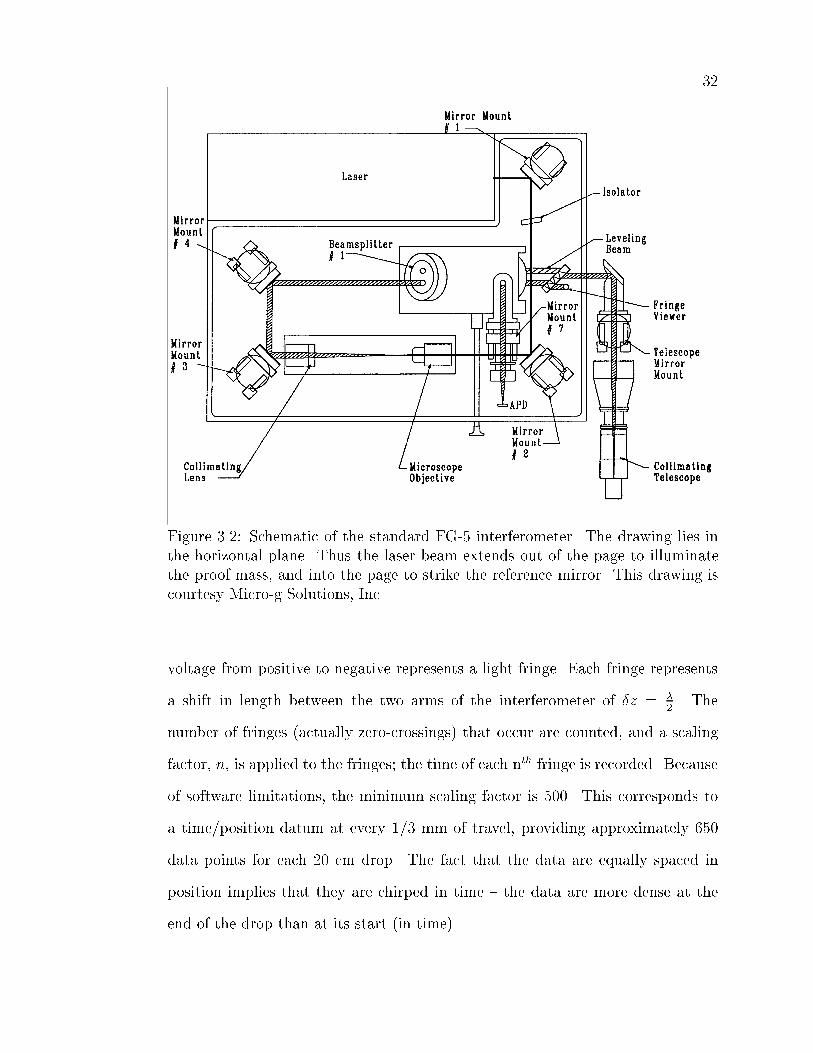
32

Figure 3.2: Schematic of the standard FG-5 interferometer. The drawing lies inthe horizontal plane. Thus the laser beam extends out of the page to illuminatethe proof mass, and into the page to strike the reference mirror. This drawing iscourtesy Micro-g Solutions, Inc.

voltage from positive to negative represents a light fringe. Each fringe represents

a shift in length between the two arms of the interferometer of �z = �2. The

number of fringes (actually zero-crossings) that occur are counted, and a scaling

factor, n, is applied to the fringes; the time of each nth fringe is recorded. Because

of software limitations, the minimum scaling factor is 500. This corresponds to

a time/position datum at every 1/3 mm of travel, providing approximately 650

data points for each 20 cm drop. The fact that the data are equally spaced in

position implies that they are chirped in time { the data are more dense at the

end of the drop than at its start (in time).

33

The stabilization scheme used to lock the laser requires that its frequency

be modulated over 6MHz at 1.2 kHz [29]. This dither is seen as a high frequency

sinusoidal position signal, but by �tting for a sinusoid at the appropriate frequency,

the e�ect of the dither on the data is minimized. Ideally the laser light would be

provided without any dither, to avoid the additional processing and �tting errors

associated with removing this signal.

As an aside, note that the errors in the measurement arising from the light

pressure of the laser beam on the test mass, time delays due to the �nite speed

of light, and Doppler shifting of the laser frequency are all common mode errors

that don't a�ect the experiment.

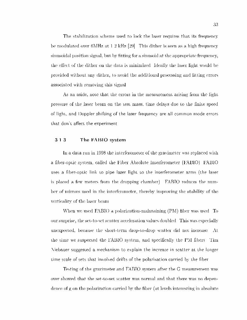
3.1.3 The FABIO system

In a data run in 1998 the interferometer of the gravimeter was replaced with

a �ber-optic system, called the Fiber Absolute Interferometer (FABIO). FABIO

uses a �ber-optic link to pipe laser light to the interferometer arms (the laser

is placed a few meters from the dropping chamber). FABIO reduces the num-

ber of mirrors used in the interferometer, thereby improving the stability of the

verticality of the laser beam.

When we used FABIO a polarization-maintaining (PM) �ber was used. To

our surprise, the set-to-set scatter acceleration values doubled. This was especially

unexpected, because the short-term drop-to-drop scatter did not increase. At

the time we suspected the FABIO system, and speci�cally the PM �bers. Tim

Niebauer suggested a mechanism to explain the increase in scatter at the longer

time scale of sets that involved drifts of the polarization carried by the �ber.

Testing of the gravimeter and FABIO system after the G measurement was

over showed that the set-to-set scatter was normal and that there was no depen-

dence of g on the polarization carried by the �ber (at levels interesting in absolute

34

determinations of g). Thus the choice to use FABIO appears to be unrelated to

the increased scatter. Section 6.1.3 includes discussion about possible sources of

the noise.

3.1.4 Phase Shifts at the Discriminator Input

Frequency dependent phase errors introduced in the fringe signal by the

electronics of the discriminator/APD system result in position/time signals that

may mimic accelerations of the proof mass. Phase shifts could be introduced

by electronic �lters or by the limited bandwidth of the APD. In the FG-5 the

APD has a bandwidth of 50 MHz so the phase errors introduced at 6 MHz (the

maximum frequency of the interferometer signal) are very small (corresponding

to a error in g of approximately 0.1 �Gal).

The phase error problem doesn't a�ect the di�erential signal unless the error

is dependent on the source mass position. We don't expect any such dependency

because the APD/�lter/discriminator circuit was positioned within the interfer-

ometer, far from the source mass and doubly shielded from its direct thermal

signature.

The fact that phase errors don't a�ect the G measurement (unless they are

truly gigantic) raised an interesting possibility. By limiting the bandwidth of the

APD circuit we could reduce its statistical noise in the measurement of the fringe

crossings. This would reduce the drop-to-drop scatter in g-values. Truncation

of the bandwidth necessarily results in phase bumps in the circuit, but in the

di�erential mode, this was not a concern. The �lter would have the same e�ect

as increasing the data sampling rate6 .

I wrote a software simulation that showed that a four-fold decrease in the

6 We could not simply increase the data density because of software limitations in the gravime-ter system. In the future experimenters would be well served to put in the work required toconvert the software system to a form that would support storage of arbitrarily dense data.

35

bandwidth (achieved by placing a low-pass �lter with a corner of 12.5 MHz be-

tween the APD output and the discriminator input) would cause only a 10 �Gal

shift in absolute gravity and negligible bias in our results. If the noise introduced

by the large bandwidth of the APD were the main source of drop-to-drop scatter

then this �lter would win a factor of close to 2 in scatter, and thus the same

factor in the integration time required to reach a given precision in G. This was

a reasonable expectation because the residuals in least squares �ts to drop data

correspond well with the actual scatter observed.

We tested a low-pass �lter at 12.5 MHz for use in a data run in 1998. The

scatter did not decrease as quickly as expected. There was no signi�cant decrease

in the size of the residuals until we used a �lter corner frequency of only 8 MHz.

Worried that the �lters were acting as antennas and injecting additional noise into

the system, we decided to forgo the use of the �lter altogether.

3.1.4.1 The Test Mass

The test mass is a complicated object designed to ful�ll several criteria. It

incorporates a mirror, a spherical lens, and a counterweight. The test mass is 9

cm long, approximately 2 cm wide, and is made of aluminum, tungsten, vespel,

glass and beryllium copper. The test mass used in the G-experiment weighed

101.2 grams. Di�erent test masses generally weigh within a gram of 101 grams.

The test mass includes a corner cube retrore ector. Corner cubes have the

property that incoming light rays are re ected anti-parallel and o�set from their

incoming paths. The re ected ray is insensitive to rotations of the corner cube so

long as the rotations occur around a point known as the \optical center" of the

cube. To minimize path length errors (and the associated acceleration bias) due

to the inevitable rotations of the freely falling test mass, the optical center of the

corner cube must as close as possible to the center of mass of the entire falling

36

object. Therefore the test mass incorporates a counterweight that is used to align

the center-of-mass to within 4 microns of the optical center of the re ector.

To allow the co-falling chamber to track the test mass as it falls, the test

mass contains a small optical glass sphere at its upper end. The sphere acts as a

lens that focuses the light of an LED onto a linear position sensor. Both the LED

and the detector are hard mounted to the co-falling chamber. The output of this

position sensor is used in the servo loop that controls the drive motor.

Three tungsten balls support the test mass on matching tungsten vees on

the co-falling chamber. Tungsten is used to reduce wear in the balls resulting

from the catch phase of the drop. The balls and vees are placed and oriented to

impart minimal rotational and horizontal velocity to the test mass at the start of

the drop. The fact that the balls do wear and change the mass distribution within

the test mass is discussed in Sec. 5.2.5.

The framework that holds these components is made of aluminum. The alu-

minum aids in reducing electrostatic forces, but is subject to eddy-current forces.

Mark Zumberge suggested constructing the proof mass from non-conductive mate-

rial, but was concerned about increasing the e�ects of thermal signals [30]. Theory

and experiment have shown that the eddy-current e�ects are negligible in normal

conditions. Because aluminum has low magnetic susceptibility the test mass is

not strongly in uenced by direct attraction to magnetic �elds.

3.1.5 The Position Reference System

A stable reference is required to make any position measurement. In the

FG-5 this reference is provided by a \super spring" one-dimensional active isola-

tion unit. The super spring was originally built by Robert Rinker as a dissertation

project with James Faller [23]. Since its conception it has undergone many re�ne-

ments, �nally resulting in the super spring used in the G-measurement. Figure 3.3

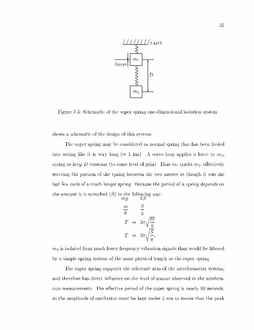
37

�� �� �� �� �� �� �� ��Earth<<<>>>

m1

<<<<<<<

>>>>>>>

m2

6

?

D

?6forcer

Figure 3.3: Schematic of the super spring one-dimensional isolation system.

shows a schematic of the design of this system.

The super spring may be considered as normal spring that has been fooled

into acting like it is very long (� 1 km). A servo loop applies a force to m1,

trying to keep D constant (to some level of gain). Thus m1 tracks m2, e�ectively

servoing the portion of the spring between the two masses as though it was the

last few coils of a much longer spring. Because the period of a spring depends on

the amount it is stretched (S) in the following way:mg = kS

m

k=

S

g

T = 2�

rm

k

T = 2�

sS

g;

m2 is isolated from much lower frequency vibration signals than would be �ltered

by a simple spring system of the same physical length as the super spring.

The super spring supports the reference arm of the interferometer system,

and therefore has direct in uence on the level of scatter observed in the accelera-

tion measurements. The e�ective period of the super spring is nearly 60 seconds,

so the amplitude of oscillation must be kept under 5 nm to insure that the peak

38

acceleration signal introduced by the reference is less than 5 �Gal. The super

spring system succeeds in this goal, an impressive achievement considering that

this corresponds to a 200-fold decrease in the vibratory acceleration signal of the

earth at the fundamental frequency of the spring. For information about how the

super spring reacts to the source mass position see Section 5.2.6.

The super spring is supported below the dropping system by a tripod (that

also holds the interferometer). There is no contact between the dropping system

and this tripod lest the vibrations triggered by the drop excite the super spring.

At the Table Mountain Gravity Observatory, where our data was taken, there was

additional isolation of the spring system. The interferometer tripod was placed

on a pier of concrete embedded7 in the oor. This reduced coupling of vibrations

through the oor.

3.2 The Source Mass

A hollow cylindrical ring-shaped source mass was �rst used in a G experi-

ment by Michael Hulett, working on a senior thesis project under Jim Faller. He

used two bronze rings fashioned from the bushings for a ship's screw propeller.

Later, in the mid-seventies, William Koldewyn8 [31] used this same pair of cylin-

ders in a G experiment that used a magnetically supported torsion pendulum. We

used the identical masses in a preliminary version of our experiment, described in

Section 6.1.1.

Hollow cylinders allow much laxer positioning requirements for G experi-

ments because they produce a gravitational �eld with extremum values, as dis-

cussed in Sec. 2.3. Figure 2.1 shows the axial acceleration �eld for a hollow

cylinder. At a certain distance from the center of the cylinder the �eld on axis

7 The piers extended approximately 5 feet below the oor, and were surrounded with Styro-foam.

8 Koldewyn also worked on his Ph.D. with Jim Faller, at Wesleyan University, 1976

39

reaches a maximal value that doesn't change with position. Thus the extrema rep-

resent areas in which the �eld is changing much more slowly than the traditional

1/r2 roll-o� of the �eld produced by a spherical mass.

The axial force is also unchanging with respect to radial translations (from

the axis of the cylinder). This is expected from symmetry considerations | the

force must get either larger or smaller (than it is on axis) as you move o� axis in

any direction. The axial force increases closer to the inner walls of the cylinder,

so the axis represents a minimum in axial force as a function of radius.

Thus a ring-shaped mass generates a �eld insensitive to translations of the

mass in any direction (at two points). The G-experiment, however, integrates

the �eld of the source mass over a �nite distance | the length of the drop.

Although the absolute position insensitivity of the �eld exists at only two points,

the extrema result in two SOD positions that maximize the perturbation to the

test mass trajectory. These positions correspond to the upper and lower source

mass positions, the one decreasing g, the other increasing it.

These properties of the source mass were essential to the success of the

experiment. Let's examine the situation if we were forced to use a spherical source

mass, and contrived to place it above and below the drop path. The di�erential

acceleration of a point test mass due to a sphere placed in two reasonable positions,

above and below the dropping region9 is strongly a�ected by positioning errors.

A 1.0 mm error in positioning would result in a signal error of 1.5%. The same

positioning error in our ring-mass system (correctly set up) would result in a signal

change of less than 0.003%, 500 times less signal error. The sphere design is not

even an option for the free-fall method.

The inner and outer radius and the height of the cylindrical source mass

9 For this example, I assume that a sphere of the same mass and density of our source masscould be placed within 4cm of the top or bottom of the drop.

40

were determined by our requirements for the experiment. If the cylinder were too

tall, for example, it would be physically impossible to place the source mass in its

lower optimal point without very drastic modi�cations to the dropping system.

On the other hand, if the mass were shorter than the greatest possible length, we

would loose signal-to-noise.

The inner radius of the source mass is roughly inversely proportional to the

signal magnitude | a smaller inner radius increases the signal. This parameter

is limited by the size of the vacuum can and the clearance required between both

the vacuum can and the co-falling chamber, and the can and the source mass. To

minimize the inner radius we constructed a thin-walled chamber with a minimum

of clearance.

The ring's outer radius a�ects both the signal size and the position of the

acceleration extrema. This choice of particular parameter was based on both

the ability of a single robust person to setup the mass, and the importance of the

additional signal achieved by increasing the radius. As the ring increases in radius

the signal gain is only linear, but the mass increases with the radius squared.

The approximate dimensions of the cylinder were 50 cm diameter, 27 cm

height, 16 cm inner radius. Our source mass weighed approximately 521 kg. This

geometry produced an acceleration signal that peaked at a value a bit larger than

43 �Gal. The total signal sensed by the gravimeter was approximately 82 �Gal.

This is smaller than twice the peak signal of the source mass because of the extent

of the test mass and the averaging action of measuring the acceleration over the

length of the drop.

Once the approximate dimensions for the ring were �xed we concerned our-

selves with limiting possible density variations throughout the mass. The most

straightforward manner of determining the density structure within an unchar-

acterized mass is to chop it into small pieces and measure the density of each

41

small bit. The amount of density information extracted depends on the size of

the bits (minced tells you more than chopped). We decided to split the mass into

12 cylindrical pieces, as in Figs. 3.4 and 3.5.

Figure 3.4: Schematic of the source mass. The source mass is constructed of non-magnetic materials including tungsten, aluminum, titanium, and bronze. Somestainless steel �xtures were also used.

Cylinders were chosen (instead of cubes, or irregular geometries) because

of their rotational symmetry and amenability to form a ring shape. Cylinders

can be characterized by more than just their density. Linear and angular density

variations can be measured (as discussed in the next Section, 3.2.1).

The 12 cylindrical tungsten billets were mounted in two levels. Cylinders

can be oriented in many ways so we were able to arrange them to best mimic a

homogeneous set; any linear or quadratic gradients in the density over the whole

height of the source mass were minimized. The gaps between the cylinders were

�lled with small tungsten rods, increasing the net density of the source mass.

Aluminum plates were used to sandwich the cylinders together. The plates

42

Figure 3.5: Photo of the source mass. The locating ring of the lower plate isclearly visible. Note how little clearance there was between the source mass andthe vacuum can.

had rims with radii three times that of the cylinders (plus � 200 �m clearance),

insuring that the masses were precisely located in the radial direction. The upper

plate provided additional strength, reducing ex of the bottom plate and defor-

mation of the source mass.

The plates were bound together with tensioning rods and bolts tapped into

the small tungsten rods. Throughout the design of the source mass we tried to

preserve as much exibility in mass positioning and support as possible, while

maintaining symmetry to ease modeling tasks. The source mass was originally

designed so that the top and bottom plate would be interchangeable, preserving

its vertical symmetry. As the experiments progressed and modi�cations were

made this symmetry was broken.

43

3.2.1 The Tungsten Masses

The tungsten cylinders were custom made for us by Schwarzkopft in Austria.

They are made of Densimet 18k | a sintered metal of 95% tungsten with 5% cop-

per and nickel as binding material. This material has good magnetic properties;

it has volume susceptibility of 0.00066 (MKS) and is paramagnetic [32, 33]. We

ordered the cylinders slightly oversized and had them �nished in house. Blaine

Horner, of the JILA instrument shop, insured that the cylinders would be as

regular as possible and dimensionally consistent from piece to piece.

The cylinders were machined to 4.080" (10.363 cm) in height and 6.530"

(16.586 cm) in diameter. Their diameters and heights are all consistent to 0.001"

(0.002 cm), with masses of approximately 39700 grams. The mean density of the

cylinders is 17.724 g/cm3 with a standard deviation of 0.008 g/cm3 ( 0.04% ). The

peak to peak density variation was 0.02 g/cm3 ( 0.12% ). Details of the cylinder

masses and volumes are provided in Appendix A.

To determine whether the cylinders were cylindrically symmetric they were

placed on an air bearing. Any inhomogeneity with angular dependence would

result in a torque along the axis of rotation. The `light' side of the cylinder was

marked and then the frequency of oscillation due to the un-balancing torque was

measured. It is possible to model an angular density variation as a bubble in the

material. With the cylinder axis oriented along the z direction

! =

rmgr

I

where ! is the angular frequency of oscillation due to a bubble of massm at radius

r. I is the moment-of-inertia of the cylinder.

The results of this test showed that 11 of the 12 masses had an angular

density variation equivalent to a 25 gram surplus at the outer radius. This suggests

that the variation is not due to bubbles (a bubble larger than 1 cc is very unlikely

44

to occur) but rather a density gradient. Such a gradient was most probably a

result of cooling e�ects. The billets were cut from 3 long cylinders that had

been cooled on their sides. It is possible to �nd out more about the angular

distribution of mass in the cylinders, but this test was su�cient to bound possible

angular density variations.

Density variations along the length of the cylinders were also measured, as

in Fig. 3.6. Given this information I was able to arrange the cylinders so that

there was only a very small net linear density change from the bottom to the top

of each layer of tungsten. This measurement was su�cient to limit linear and

quadratic density dependence along the height of the whole source mass.

Using the information about density variations from one cylinder to the

next, from one side of each cylinder to the other, and from their tops to their

bottoms, I was able to make an error estimate for the assumption (made in our

models) that the masses were homogeneous. The error from this source forms

approximately a quarter of our net uncertainty. In a new experiment I would

suggest constructing the source mass out of much smaller cylinders, spheres, or

cubes than we used this time around. By decreasing the size of the individual

components density variations could be better controlled.

3.2.2 The Drive/Support Structure

The support structure for the source mass consisted of a large aluminum

tripod that supported three screws synchronously rotated by a stepper motor.

The tripod was designed to allow easy disassembly for transportation purposes.

Each leg was bolted into a thick \main plate" that formed the acme of the tripod.

The legs had adjustable leveling feet. Tensioning wires ran from the plate to the

legs increasing the rigidity of the structure and preventing twisting motions.

On top of the main plate of the tripod rested the \drive plate" that sup-

45

Figure 3.6: Photo and schematic of the pivot and balance system used to measuredensity variations along the length of the tungsten cylinders. Two 3/4" ballbearings were used to de�ne the pivot line.

ported the screws and drive structure. The drive plate could be moved 2 cm in

the horizontal plane to position the source mass concentrically with the dropping

46

chamber (clearance for the screws was cut into the main plate). The drive plate

was also equipped with a central retractable pivot that could be used to produce

a pure rotation of the plate and screws in the vertical direction. This degree of

freedom was incorporated in the design to insure that the screws could be posi-

tioned about the FG-5 with maximum clearance. After position adjustments the

drive plate was clamped to the main plate to prevent creep.

The screws were supported by bolts riding on cylindrical roller bearings

located in aluminum towers bolted to the drive plate (Fig.3.7). The towers provide

space for a secondary set of cylindrical roller bearings that increased the rigidity

with which the screws were held. Attached to each screw was a plastic sprocket

keyed to prevent slippage. The three screw/sprocket assemblies were linked to

each other with a stainless steel chain that was annealed to reduce its magnetic

susceptibility. This chain cycle was driven by a sprocket rotated by a separate

chain loop connected to a stepper motor. This constrained the screws to rotate

synchronously (in the limit that there was no slack). The worst case phase shift

between screws is equivalent to a single link misplacement because the sprockets

provide, in some sense, a quantized positioning mechanism. Even this worst case

shift was negligible.

The stepper motor was bolted to the main plate of the tripod as far from the

FG-5 as possible. It was held with vibration isolating mounts The drive chain was

turned through a rubber shaft attached to the motor. These isolating measures

were taken to minimize the vibration of the ground due to the drive system,

which could disturb the gravimeter. Although the vibrations were of too high a

frequency to excite the super spring much, no vibration is good vibration.

47

Figure 3.7: Photo of the screw drive/support system. A) The drive plate. B) Themain support plate. C) A tower supporting one of the screws. D) One of threeclamps.

3.3 Superconducting Relative Gravimeter

Local acceleration may be a�ected through many mechanisms10 . Atmo-

spheric e�ects, for example, can change in gravity either by changing the mass of

the air above the observation site, or by compressing the ground11 . This signal

has been calculated to be approximately -0.40 �Gal /mbar at Boulder ([24, 35]).

Tides, ground water changes, continental uplift and ocean loading can change

gravity as well. Tides, by far the largest source of gravity signals (� 150 �Gal),

occur on a much longer time scale than the modulation of our source mass. Tides

10 People have thought of many ways gravity measurements may be a�ected. It has beensuggested that atmospheric pressure associated with solar eclipses could a�ect gravity[34]. Theumbra moves with supersonic speed across the surface of the earth, creating a transient pressuredisturbance due to the decrease in air temperature within the sunspot. The pressure changewould then change the value of the local acceleration. Luckily solar eclipses don't happen everyfew minutes!

11 The corresponding change in the distance to the center of the Earth increase the localacceleration.

48

are approximately biurnal (6 hour period), while our source mass position was

alternated every 20 minutes, at the slowest. Thus tides did not correlate strongly

with our signal. Some faster environmental signals, however, might have randomly

correlated with the source mass position and increased the scatter in our results.

These signals would not have systematically biased our �nal value.

To avoid unnecessary scatter we used a superconducting relative gravimeter

(SRG) to record real time varying gravity signals concurrently with the G ex-

periment. The SRG cannot provide an absolute value for the local acceleration

(something like 9.8 m/s2) but can only track relative changes in g. For example,

between time t and T , the relative meter might give a measurement equivalent to:

g(T ) = g(t)+12:345 �Gal. We subtracted the gravity signal (as recorded with the

SRG) from the acceleration values extracted from the absolute drop data. This

reduced the scatter introduced into our experiment by real time varying gravity

signals due to environmental sources.

The SRG works by measuring displacements of a mass on a spring. As

the local gravity decreases, the mass is lifted by the spring. As the local gravity

increases, the spring is stretched, lowering the mass. The change in equilibrium

position can be related to the change in the weight (due to the change in gravity)

of the mass through Hooke's law. A schematic of the system is seen in Figure

3.8. The mass in the SRG system is a superconducting niobium sphere and the

spring is actually provided by a magnetic �eld generated by persistent currents

running in two superconducting coils. The motion of the equilibrium position of

the sphere is recorded with an AC capacitance bridge surrounding the sphere.

The spring constant of the SRG system must be calibrated before the po-

sition of the spring/mass equilibrium can be related to changes in gravity. The

output can be calibrated in a variety of ways, but the SRG we used was calibrated

49

Figure 3.8: Schematic of the superconducting relative gravimeter used to recordreal time varying gravity signals. This drawing is courtesy GWR Instruments.

from another SRG12 . The two systems were placed side by side and allowed to

measure environmental signals concurrently. Comparison of the results completed

the calibration. Any errors in the calibration would lead only to residual environ-

mental signals in our data. It is important to note that the SRG system could not

remove time varying signals arising from drifting errors in the free-fall gravimeter

12 This second SRG was previously calibrated with a mechanical system that physically ac-celerated the entire SRG apparatus at known rates. Both calibrations were done by NOAApersonnel independently of the G-measurement. The quality of the SRG raises the question\Why not do the free fall measurement with out the free fall? Just use a SRG." This is byno means an unreasonable question, and in fact the idea is good. There is no reason why thisexperiment should not be carried out. One issue that limits the utility of the SRG for a Gmeasurement, however, is the di�culty of calibrating the output. Currently SRGs can only becalibrated to several parts in 104.

50

system that actually recorded the acceleration signal of the source mass.

The SRG is subject to drifts and steps in its output. Some drifts result from

mass changes of the niobium sphere (it adsorbs helium). Throughout our data

run we performed linear least squares �tting for the drift and determined that it

was less than 0.2 �Gal per day | having negligible impact on our values for the

G.

CHAPTER 4

ANALYSIS

A central task that we faced with the free fall method was implementing the

software system used to extract G from gravimeter data. This chapter describes

the algorithms we used to this end. Preliminary work was discussed in Chapter

2. Section 2.1 included the calculation of mutual attraction of the test mass and

source mass over the large range of relative positions in which they are placed. In

Sec. 2.2 the method of numerically integrating the equation of motion of the test

mass was presented.

4.1 A Big Least Squares Solution

A statistically correct way to extract G from observed data is to calculate

a least-squares solution in which G is a �tting parameter of the problem.

One might imagine �tting the parabolic path of the dropped object to a

function, z(t) composed of a standard solution for a falling object (as in Section

2.2), and a term explicitly dependent on G:

z(t) =1

2g(t2 +

t4

12) + V0(t+

t3

6) +X0(1 +

1

2 t2) + G f(t)

where f(t) is a basis function describing the e�ect of the gravitational interac-

tion between the source and proof masses. Unfortunately this was not reasonable

because f(t) looked very much like a parabola; the correlation between the per-

turbation we were trying to measure and the e�ect of the local acceleration was

52

strong (as is evident in Fig.2.2). For this reason the problem had to be posed with

the di�erential nature of the data evident. We did this by folding all the informa-

tion from drops with the source mass in both positions into one \big least-squares

solution" (LSS).

The LSS had to convert the information of the observations (the posi-

tion/time points for each drop), the superconducting relative gravimeter (SRG)

data (essentially an acceleration value), and the gravitational signal of the source

mass into a single form that would allow them to be compared. Least-squares

�tting minimizes the total chi-squared error between individual data points and

a �tting function. In our case the individual data points were position/time pairs

from drop data. The �tting function was a fourth-degree polynomial describing

the motion of a freely falling object in a simple gravity �eld (Eqn.2.10).

It is not immediately clear how all this information can be combined to

generate a chi-squared value that depends on the choice of the �tting parameters.

The problem was complicated by the many di�erent relationships between the

observations and the various �tting parameters. For example, Xo; Vo, and g are

local to the data within a single drop. On the other hand, the variable G, the o�set

from the SRG from the absolute local acceleration (O), and a drift parameter

for the SRG, D1 , were global to the whole problem. An individual datum is

associated with all the other data of its drop in one way, in a di�erent way with

data sharing the source mass position, all the remaining data in yet another way.

Even data within a single set is separated in time | environmental gravity signals

change appreciably on a time scale of minutes.

The LSS began with the removal of the laser dither signal from the drop

1 To remove environmental signals, data from a superconducting relative gravimeter (SRG)is included in the procedure. Unfortunately relative meters can only give information aboutchanges in local gravity { an o�set between the relative value and the absolute value must beincluded in the �t. Relative meters also su�er from small drifts, which must be �t for as well.See Sec. 3.3.

53

data. The dither of the laser signal (Sec. 3.1.2) correlated very weakly with G,

which is why it was dealt with before applying LSS. Fitting the data of each drop

for:

z(t) =1

2g0(t2 +

t4

12) + V0(t+

t3

6) + Z0(1 +

1

2 t2) + A sin!dt+B cos!dt

where !d is the dither angular frequency (� 1200 Hz), allowed only the dither

signal to be removed. Note that this \pre-cleaning" was only possible because the

dither basis function was of such high frequency that it was nearly orthogonal to

the other basis functions.

The �t for the dither provided starting values for g', V0, and Z0. These

values were used to set up the design matrix of the problem. g0 was corrected

with the acceleration value from the super conductor, gsc, appropriate for the

time of the drop. g0 was also corrected with the global values of the o�set and

drift:

ge�ective = g0 +O +Dt+ gsc

The design matrix also must include information about our gravity signal.

This was included, for each datum, by integrating the equation of motion (Eqn.

2.11) with the global value of G. It was the position value returned by this inte-

gration that was used in the design matrix for the G parameter.

Since the base unit of information dealt with in the LSS was a single position-

time datum and because there were more than 650 such data per drop, and more

than 150,000 drops in our data sets, the least squares matrix was necessarily large.

The matrix resulting from our set up had more than 16,000,000 observations and

requires nearly 200,000 adjusted parameters. Dealing with such a large matrix

requires greater addressing capacities than possessed by desktop computers |

extra cleverness is required.

54

Because none of the parameters local to a drop were correlated with the

equivalent parameters of other drops, the design matrix was sparse2 . The matrix

was therefore largely empty; it had a banded-block structure, in which the only

non-zero elements of the matrix were in bands at its edges and in blocks along its

diagonal. Algorithms developed to deal with sparse-matrices made the problem

tractable { it could be solved in about two weeks with a desktop workstation

[36, 37].

4.2 The Method of Parallels

A more intuitive method of extracting the value of G from the observed data

exists. The method of parallels (MOP) was faster than the LSS, but included less

information about correlations between the initial conditions of drops and the

value of G. In MOP a theoretical prediction of the change in observed gravity due

to the source mass was compared to a measured change in g.

MOP required that an assumed value of the constant of gravity, Gt, be

adopted so that the magnitude of the source mass signal on the measured local

acceleration could be predicted. The prediction, �gt, was found by �tting parabo-

las to theoretical position-time curves3 generated modeling the source mass in its

two positions. The magnitude of �gt was linear in Gt so it was easily related to

an experimentally observed change in gravity, �go:

�gtGt

=�goG: (4.1)

Of course the �tting functions used to generate the prediction of the signal had

to be the same functions used to �t the actual drop data.

It was only because G correlated so weakly with the other parameters of the

2 Only the value of the constant, the value of the o�set to the relative meter, and its driftwere global to the whole problem.

3 Describing the motion of the test mass, as generated in Sec. 2.2.

55

free-fall problem that MOP was successful. As we saw from the correlation ma-

trices from the LSS4 , the correlation between G and any other �tting parameter

(used in the LSS) was less than 0.1. MOP didn't juggle all the information we had

in a single least squares solution, but the information it dealt with was su�ciently

independent to allow the solution to be partitioned. First the position/time pairs

of each drop were �t for an acceleration value. Second an analysis of the acceler-

ation values produced a �go value. Third �go and �gt were compared, producing

a value for G. Because LSS and MOP produced highly consistent results, MOP

was used in the �nal analysis.

4.2.1 Di�erencing Techniques

We used a variety of methods to extract the experimental �go value from the

data. The simplest way to calculate the di�erence was to subtract the average the

value of the local acceleration measured with the source in its lower position from

the average with the mass in the upper position. This method is not optimal;

it does not recognize underlying time varying signals in the local acceleration

resulting in increased scatter.

A second method that we used involved taking individual di�erences, as

shown in Fig.4.1. This was essentially the same as the �rst method, but allowed

identi�cation of outlying di�erence values, so that they could be removed. With

this method the di�erences we measured were not completely uncorrelated | each

set of data was used to calculate two di�erence values. Therefore we had to be

careful in our analysis of statistical uncertainty.

We used a third method to avoid the e�ects of linear drifts on the scatter of

the di�erences (Fig.4.1). It involved estimating the drift of the local acceleration

across three sets of data by averaging two consecutive sets that shared a common

4 And qualitatively from self-consistency tests with MOP.

56

:::::::::p p p p p p p p p p p p p p p p p p

:::::::::p p p p p p p p p p p p p p p p p p p p p p p p p p p p p p p p p p p

:::::::::

p p p p p p p p p p p p p p p p p p p p p p p p p p p p p p p p p p p :::::::::

:::::::::

:::::::::

Method 2

XXXXXXXXX

Method 3

-Time

6

Acceleration

Figure 4.1: Two methods of calculating �go given acceleration data. (:::::) repre-sents a set of acceleration data with the source mass in either its upper or lowerposition. The vertical lines represent the measured di�erence value associatedwith the pair or trio of sets.

source mass position. By taking the di�erence of this average with respect to

the intervening set (with the source mass in its other position), the e�ect of

linear drifts on the di�erences was minimized. Method three had even stronger

correlations between the di�erences than method two, for three di�erence values

shared information from one set.

A statistically correct implementation of the third method was used in our

�nal analysis. First uncertainty values were associated with the time and accel-

eration of each drop, allowing the importance of the information of each drop to

be appropriately weighted. The uncertainty value was based on the chi-squared

value of the parabolic �t to that particular drop. A line was �t, with linear least

squares, to each pair of subsequent sets sharing a common source mass position.

Then the weighted mean of the intervening set was removed from the value of the

line at that time5 . This system produced a statistically correct estimate for the

error in each di�erence value. The �nal �go was formed by the weighted mean

5 There is no reason that the time of each drop cannot be weighted according to the uncer-tainty of the drop. Thus it was possible to associate a \weighted mean time," a single time bestrepresenting the data in the set.

57

value of these di�erence results, with an error estimate taken from the weighted

mean standard deviation of the individual di�erences.

4.3 Dependence of �go on First Fringe Fit

The methods of MOP and LSS destroyed a great deal of information. MOP

reduced the approximately 96 billion position/time pairs of the experiment into a

series of less than 2000 measurements of the experimental �go. These di�erences

were then averaged to return a signal best estimate for �go. Yet it was possible

to extract other information about the free-fall system. This section outlines an

approach (using MOP) that I used to extract information about the position of

the source mass with respect to the SOD position. In Secs. 3.1.1.2 and 5.1.2 an

alternate \direct" measurement of the SOD is presented.

The gravimeter system recorded approximately 650 usable position/time for

the test mass during each drop. By varying the set of data within each drop that

was �t the SOD could be found by analysis of the dependence of �go on the choice

of the sub set. A reasonable manner of altering the subset was to change the �rst

or last fringe that was �t. It was more useful to modify the �rst �t fringe (FFF)

than the last �t fringe, because the e�ect of the acceleration parameter is most

obvious at the start of the drop.

The �go value extracted from the data had a very similar dependency on

the FFF as the acceleration �eld of the source mass had on position. Imagine

an acceleration �eld that contains a step increase occurring in the middle of the

drop region (in the spatial middle of recorded data). As the FFF approaches this

step, the extracted value of g will increase. As soon as the �rst fringe is beyond

the step, the value of g will no longer change with the fringe number. Clearly the

position of the step can be determined by analysis of the gravimeter data.

In a very similar manner the changing (in space) acceleration �eld of the

58

source mass left a signature dependence of �go on the FFF. By comparing the-

oretical curves, generated assuming di�erent SOD positions, to the observed de-

pendence, a best-agreement SOD position was found6 . Fig. 4.2 shows the quality

of agreement for di�erent SOD positions on di�erent days of the experiment. By

scaling the best-�t theoretical curve, generated at the extracted SOD, to the data

(with a single multiplicative factor), a scaling of theoretical value of G used in our

models could also be made.

−0.4 −0.3 −0.2 −0.1 0 0.1 0.2 0.3 0.40

0.2

0.4

0.6

0.8

1

1.2

1.4

1.6

1.8

2

Start-of-drop position, cm

Fitquality

Figure 4.2: Here the quality of a �t of theoretical data to experimental datais plotted. The curves that were �t represented the dependence of �g on theFFF in the position/time data recorded by the gravimeter. Each line plottedhere represents the quality of the agreement between theory and experiment,for a particular day of the 1998 experiment. The weighting/quality assessmentwas based on the chi-squared value in a linear least squares routine that �t thetheoretical curve (at a given start-of-drop position) to the experimentally derivedcurve. The �t was in one-dimensional (for a scaling factor).

Noise in the data results in greater and greater deterioration of the �go value

extracted with less and less data �t 7 . This constrained the region over which the

6 In the free-fall measurement the translation of the source mass between its upper and lowerpositions was very well known compared to the mass's position relative to the SOD.

7 There are two reasons for this deterioration. The �rst is that the statistical uncertainty

59

FFF was varied to the fringes between the earliest usable data in each drop and

the fringe where the uncertainty in �go became large. We were fortunate that this

sub-set encompassed the region where the second derivative of �go with respect to

the FFF was greatest. If the second derivative were small the correlation between

the scaling factor for the theoretical G and the SOD position would increase, as

would the uncertainty in the best-�t SOD value.

This method to �nd the SOD position was applied to two independent

data runs. In the �rst run the extracted SOD position was consistent with the

\direct" measurement (Sec. 5.1.2). In the second run, however, the two values

were inconsistent, disagreeing by nearly 2 mm | about 4 standard deviations. I

attribute this discrepancy to the fact that in the second data run changes in the

shaft-encoder voltage were monitored. Conceivably, as in quantum physics, the

observer a�ected the observed, and changed the SOD position. Thus the extracted

SOD position was used for the �nal determinations of G in both data runs.

The extracted SOD value is more appropriate than the direct value. Exam-

ination of the values of G obtained for a set of FFF values for the two di�erent

SOD positions results in Figure 4.3. There is no physical dependence of G on

FFF, but the directly reference value suggested that there is | because the direct

reference was incorrect. Note that the G values extracted for FFF about fringe 18

agree well between the two SOD positions. This agreement is due to our lack of

sensitivity to positioning errors, and is a consequence of the extrema of the source

mass �eld. In some sense the positioning error doesn't matter if a reasonable FFF

is chosen for analysis.

To check for a systematic drift or signal in the SOD position during a data

run (conceivably due to ball wear, Sec. 5.2.5) the best-agreement SOD position

(inversely proportional topN where N is the number of data points �t) increases. The second

is that the correlation between g and the other �tting parameters increases as the beginning ofthe drop is excluded from the �t.

60

0 20 40 60 80 100 120 140 1606.63

6.64

6.65

6.66

6.67

6.68

6.69

6.7

6.71

6.72

First fit fringe

G X

1011

m3 /k

g−s2

Figure 4.3: The value of G extracted from the data as a function of the �rst fringe�t. The points marked with asterisks are generated using the SOD value extractedfrom drop data. The points marked with crosses use the directly referenced SODposition. The small points bounding each set of error bars show the G value usingthe appropriate SOD �1�.

for each day is plotted in Fig.4.4. There is no signi�cant drift. There is also no

correlation between the value of G produced by a day of data, and its best-�t

SOD.

61

140 145 150 1554.6

4.7

4.8

4.9

5

5.1

5.2

5.3

5.4

Day of experiment

Ext

ract

ed d

rop

posi

tion,

cm

Figure 4.4: The start-of-drop position extracted from each day of the 1998 experi-ment. The error bars are based on the chi-squared agreement of the least-squares-�t of the data to theory. The error bars are used only for weighting purposes.The horizontal line shows the weighted mean position.

CHAPTER 5

ERROR ANALYSIS

All mechanisms that introduce errors to the G experiment lead to one result

| the breakdown of the connection between the theoretical model of the experi-

ment and its physical reality. The careful calculation, determination, and, in some

cases, estimation of the magnitudes of the errors associated with our experiment

is of the utmost importance in describing our results. Because the standard used

to evaluate the level of agreement between experimental results is the number of

standard errors between their values (the t-test), the uncertainty associated with

our results will a�ect the way we perceive agreement levels.

A discussion and summary of the main sources of error in the free-fall ex-

periment is in presented in Section 5.1. I have chosen to present some systematic

error sources in depth in section, Sec. 5.2. Some techniques that we have used to

search for indicators of systematic errors are presented in the last section of this

chapter. The \hard" presentation of signi�cant errors, including the values used

in determining their magnitudes is provided in Appendix B.

5.1 General Error Analysis

5.1.1 Common mode errors

Many error signals fall into the class called \common mode". These signals

a�ect the absolute accuracy of the FG-5 system, but have little impact on its

63

di�erential precision. Mechanisms that in uence the absolute accuracy of the

gravimeter are easy to imagine|and become even more so when you start trying

to think of errors capable of acting on the gravimeter di�erentially.

Consider the e�ect of the building that housed the experiment. This building

certainly a�ected the acceleration of the test mass, probably at the level of 5 �Gal

in the common mode. Yet we don't expect it to introduce a change our measured

source mass signal on a level greater than 5 parts in 109 because it was on this

level that the di�erential equation describing the motion of the test mass was

invalidated. A general list of common mode e�ects that are not important in the

di�erential mode includes:

� gravitational attraction of the co-falling chamber

� drag e�ects of residual gas in the vacuum

� light pressure of the laser sensing the test mass position

� forces due to magnetic �eld of the earth

� gravitational attraction of stationary apparatus

� slowly varying gravitational e�ects due to:

|Lunar Tides

|Earth Tides

|Ocean Loading

|Atmospheric pressure changes

|Water table changes or snow fall

|Temperature drift e�ects

|Continental uplift

� slowly varying machine dependent drifts:

|Laser verticality

|Laser frequency or time standards drifts

64

|Laser intensity changes

|Vacuum pressure changes

Although common mode errors don't bias our results, they could strongly

in uence the scatter in the free fall measurement if they modulated the g-signal

on a time scale close to the source mass modulation. Two data runs with di�erent

modulation rates were made. The �rst, in 1997, modulated the source mass

every twenty minutes. During the �rst 17 minutes of each \set", 100 drops were

measured with 10 seconds between each drop. In a second data run in 1998,

the source mass was modulated at 11 minutes, with 90 drops per set (5 seconds

between drops). Scatter in this second data run would only be strongly sensitive

to common mode signals changing at periods less than about 30 minutes.

5.1.2 Positioning Errors

Errors made in positioning the source and proof masses resulted in system-

atic errors that were not ameliorated by the di�erential nature of the experiment.

The analysis of these positioning errors is divided into a treatment of the source

and proof masses separately.

Errors in the source mass vertical position with respect to the start-of-drop

(SOD) biased the calculation of the acceleration experienced by the test mass and

our value of G. This type of errors was introduced by wear in the support nuts of

the source mass, by inaccuracy in referencing the mass to the vacuum chamber,

and uncertainty in the SOD position within the chamber. Because we operated

at the extrema positions of the source mass �eld, however, positioning errors were

not a major source of error in the experiment. The uncertainties associated with

the source mass positioning issues are fully presented in Sec. B.1.1, in Appendix

65

B. The net e�ect of vertical positioning errors was only 10 ppm.

Error positioning the tungsten cylinders within the source mass was a much

more important source of uncertainty. Because the radial position of the large

tungsten cylinders was determined by the locating lip of the sandwiching plates

(which allowed some clearance) the cylinders' radii from the drop were not abso-

lutely de�ned. The plate that supported the tungsten mass distorted under their

weight producing additional uncertainty. Density inhomogeneities, so carefully

dealt with in Sec. 3.2.1, had the same e�ect as misplacing elements of the source

mass. These sources of error were responsible for nearly 100 ppms of uncertainty.

The complicated proof mass, which underwent free fall motion, was a greater

source of positioning errors than the source mass. Most important was the radial

position of the proof mass, which depended on horizontal velocities (that could

never be made identically zero), and the centering of the proof mass within the

dropping chamber. Estimates of radial positioning errors were made with a sim-

pli�ed model of the proof mass that was increasingly miss-positioned horizontally.

The variation in acceleration signal with the radial o�set of the proof mass from

the symmetry axis is roughly quadratic. Figure 5.1 displays the e�ect on the

vertical acceleration of the proof mass by moving it o� the axis of symmetry of

the source mass.

The proof mass optical center was \directly" referenced to the source mass

only through a long chain of measurements:

� Optical center of corner cube to tungsten balls (within test mass)

� Tungsten balls to tungsten vees (test mass {> co-falling chamber).

� Tungsten vees to bottom of co-falling chamber.

(within co-falling chamber).

� Co-falling chamber to stop at bottom of dropping chamber.

66

−20 −10 0 10 20 30 40−0.025

−0.02

−0.015

−0.01

−0.005

0

0.005

0.01

0.015

0.02

0.025

Position, cm

Accelerationdi�erence,�Gal

Figure 5.1: Di�erence in vertical acceleration (due to the source mass) sensed bya simple proof mass (8 cm long hollow cylinder with 1 cm diameter and 1 mmwall) falling on axis and (|) 0.1 cm, (�{�) 0.2 cm, (� � �) 0.4 cm o� axis. Positionis with respect to the source mass. Note that radial position errors have preciselythe same e�ect as a scaling of G.

assembly (via shaft encoder servo).

� Gravimeter bottom stop to bottom of gravimeter vacuum.

(within drop chamber) chamber.

� Bottom of dropping chamber assembly to top of lower ange on

vacuum can.

� Top of ange to bottom of the source mass

in its lower position.

These measurements were made directly1 , with the vacuum chamber open to air.

This trail of references added error at every step. Alternatively information about

1 For the most part. The shaft encoder travel to the SOD was interpolated from the diameterof the drive pulley and calibrations of the shaft encoder output.

67

the position of the test mass could be extracted from the data (as in Section 4.3).

In a data run in 1997 experiment the two independent determinations (ex-

tracted and directly measured) of the position agreed well, but in another run

in 1998 they were not consistent. The set-to-set variation in the position, as

measured by the shaft-encoder, was the same magnitude as this disagreement (in

the 1998 experiment). Possibly the system that was used to monitor the shaft-

encoder voltage throughout the 1998 measurement may have a�ected the system.

For these reasons we adopted the position value extracted from the data (Sec.

4.3 includes a discussion of why this was reasonable). Using the value given by

the \direct" measurement changes the �nal value by less than 1/2 sigma.

5.1.3 Modeling Errors

Errors in the measurement of masses contributed weakly to our �nal error

estimates. The direct measurement of the masses of the tungsten cylinders and

the two aluminum plates was the largest source of error. Buoyancy corrections

were applied for these objects (Sec. B.3.1). The smaller components of the

source mass (nuts and bolts) could be weighed with higher precision because of

their small mass. The total uncertainty associated with errors of this type was

about 40 ppm.

Although the total mass of the test mass had no bearing on the acceleration

di�erence we measured, its mass distribution did. Thus it was important that the

relative densities and positions of the various components of the test mass were

correctly modeled. Although there was essentially no error introduced during the

modeling of the source mass2 , modeling the test mass was very di�cult because of

the complexity of its design. Errors in the relative masses (� 0.05 g) and positions

2 Certain approximations were made during the modeling of screw threads, bolt heads, andgroups of bolts, as discussed in Appendix A. These approximations were very good.

68

(� 0.01 cm) of the components of the proof mass contribute about 90 ppm to our

uncertainty.

Over the course of the free fall experiment the tungsten balls that supported

the test mass experienced some wear. This introduced three errors: Firstly a

change in the relative mass of the balls to the rest of the test mass, secondly a

change in the mass distribution within the balls themselves, and thirdly a change

in the SOD position. These are all very small errors, and are discussed in Sec.

5.2.5.

5.1.4 Numerical Techniques

A primary assumption of the free-fall method of measuring G was that the

theoretical framework we built was accurate enough to describe the experiment to

better accuracy than it could be carried out. Position versus time data for the test

mass lacked meaning if we could not relate them and their variations to the source

mass and G. There were many levels at which our numerical approximations may

have di�ered from reality. I think it reasonable to start the discussion of possible

errors with the integration over the source mass.

The Romberg quadrature algorithms we used to evaluate the integrations

over the source and proof mass incorporated an error estimating functionality (Sec.

2.1). We speci�ed that the individual integrations return a value good to better

than 1 part in 108. The individual integrations agreed at this level with analytic

test cases. The error introduced by this limit of accuracy was overshadowed by

the approximation we made in integrating over an interpolation �eld (Sec. 2.1).

By specifying a su�ciently dense grid, however, this source of error could be

controlled to arbitrary precision. The �nal grid precision we used corresponded

to an uncertainty of 20 ppm.

To reduce the interpolation �eld to a two-dimensional grid we assumed that

69

the gravitational �eld produced by the source mass was cylindrically symmetric.

This was very good approximation to a level of 20 of ppm.

5.1.5 Spurious Signals

Thermal and magnetic e�ects were among the hardest sources of uncertainty

to quantify. These sources of discussed in depth later in this chapter, within Sec.

5.2. Here a very brief discussion is included.

We had to perform secondary experiments to get the magnitude of signals

arising from these two areas. A test for thermal e�ects was made by placing

modulated heat sources around the gravimeter, recording the power incident on

the gravimeter and the resulting g signal. The modulation frequency matched

the modulation rate in the 1997 experiment, 20 minutes per set. This would

overestimate the thermal signal in a 1998 data run in which only 11 minutes were

allocated per set.

We bounded the magnitudes of the magnetic signals both by calculating the

e�ect (for eddy current damping during the drop) and by experimentation (for

the force of the magnetic AC signals). The theoretical calculations were based

on measurements of the DC magnetic �eld in the region of the dropping chamber

and on the susceptibility and (simpli�ed) geometry of the source and test masses.

The experiment is presented in Sec. 5.2.8 on page 96.

5.1.6 Contaminated Data

There were several ways data could be ruined. Earthquakes resulted in

huge scatter in the measurement of acceleration values. When the scatter was

large enough (several hundred �Gal ) the source mass signal could be completely

swamped out. Occasionally fringes were miscounted, ruining individual drops

(Sec. 5.2.9, pg. 101). Rarely the laser lost its frequency lock, resulting in a

70

position measurement made with a uncalibrated \ruler".

Drops contaminated by missed fringes were easily identi�ed and removed

from the set of drops used in the di�erencing. Some unreasonable data was not

so obvious. The criterion that we chose to remove this data was simple: Drops

that produced g values more than 3 standard deviations from the mean g-value

for the particular set were removed.

Our treatment of earthquake contaminated data was even more casual.

Earthquakes were removed by eye. Generally just the beginning of the earthquake

was removed, leaving several sets with large scatter due to the motion of the su-

per spring. The di�erence values produced from these sets were \automatically"

associated with greater uncertainty with the di�erencing algorithm discussed in

Sec. 4.2.1. Entire earthquakes were left in the data to test the method, and

no signi�cant change (> 0:2�) in any days' G result was observed. Figure 5.2

summarizes our feelings about earthquake contaminated data.

Totaled Non-statistical Error Estimates

Table 5.1 presents a summary of the major systematic error sources of the

free-fall experiment. The table is split into two sections for the two data runs

because some errors were better controlled in the 1998 run.

5.2 Sources of Systematic Error

There are many sources of real gravity changes that are sensed by free

fall and super conducting gravimeters (tides, atmospheric signals, water table

changes. . . ). These sources do not complete the set of mechanisms that in uence

measured gravity; instrumental errors are sources of false signals that can have

equal bearing on the results of the acceleration measurement as real gravitational

e�ects. All the systematic non-gravitational signals we have discovered in the

71

Figure 5.2: A Hallmark postcard { commentary on our data analysis technique?Because our results don't change by more than a tenth of a standard uncertaintywhether we take or leave the little fellow, we don't think it much matters.

72Source of Uncertainty 1997 Error 1998 ErrorPositioning Errors

Vertical positioning 10 ppm 10 ppmRadial positioning 85 ppm 60 ppmInternal positioning 85 ppm 45 ppmRSS TOTAL: 120 ppm 75 ppm

Modeling Errors

Granularity of mass models 52 ppm 52 ppmSymmetry Assumption 20 ppm 20 ppmInterpolation Density 20 ppm 20 ppmModeling 90 ppm 90 ppmSource mass density variations:Point mass 60 ppm 60 ppmLinear 50 ppm 50 ppmQuadratic 60 ppm 60 ppmAngular 25 ppm 25 ppmRSS TOTAL: 145 ppm 145 ppm

Thermal Signals 60 ppm 60 ppmAirgap 75 ppm 75 ppm

Table 5.1: A table of the magnitudes of the important error sources. Error esti-mates are separated between two data runs in 1997 and 1998. Generally the errorestimates are the same or better in the 1998 run because this run incorporatedmore robust support plates for the source mass and more precise alignment of thesource mass and dropping system.

free fall G-measurement were consequences of di�erential modulation of these

mechanisms.

This section contains discussion of some sources of error in the measurement

of the local acceleration, and the manner that the G experiment might modulate

the errors to create systematic bias in our results. The subsections are arranged

by the magnitude of the uncertainty due to the mechanism. One or two of the

subsections discuss broader subjects than a single error source (Secs. 5.2.9 and

5.2.10 ).

More complete discussion of all the error sources (including common mode)

73

in the free fall gravimeter may be found in [30, 24, 38]. Only errors springing

from the FG-5 system are discussed here because we don't expect (or see evidence

of) any systematic connection between the free fall measurement and the super

conducting system.

5.2.1 Air Gap Modulation

Because the dropping chamber is in high vacuum whilst the rest of the

gravimeter is in air, an air-vacuum interface exists between the arms of the in-

terferometer. The index of refraction of air is slightly larger than the index of

vacuum, so motions of the interface (the \airgap") result in phase shifts of the

fringe signal[39, 38]. If the interface moved upwards by an amount � the laser

beam would pass through a distance � where vacuum had been replaced by air.

This would result in a phase shift mimicking a motion of the test mass upwards,

away from the interface. If the interface moved downwards, there would be a

corresponding false motion of the proof mass towards the interface.

At the start of the drop the co-falling chamber is accelerated quickly from

rest jarring of the dropping chamber and introducing a vibration in the airgap that

couples into the g measurement in just this way | these vibrations necessitate the

separation of the interferometer/spring system from the dropper least the super

spring be excited. Figure 5.3 is a plot of the vertical position of the interface as a

function of time averaged over 90 drops.

This noise signal is systematically linked to the drop | it is triggered by the

drop motion. Power spectral analysis of the motion (Figure 5.4) shows that the

airgap motion might be modeled as a sinusoid with frequency 63 Hz (a very bad

approximation). A sinusoidal motion at this frequency has a small but non-zero

correlation with the acceleration parameter of the linear �t for gravity.

The e�ect of the airgap modulation was not completely common mode be-

74

0 0.05 0.1 0.15 0.2−8

−6

−4

−2

0

2

4

6

8x 10

−5

Time, seconds

Ver

tical

pos

ition

, cm

Figure 5.3: Vertical motion of the air-vacuum interface between the droppingchamber and the interferometer. This trace was averaged over 90 drops of the testmass. The two vertical dotted lines represent the typical start and stop positionsfor the �t for local acceleration. Note that the mean position of the interface isnon-zero during the drop because the test mass and its co-falling chamber becameweightless during each drop causing the rest of the tripod/dropping assembly tojump up on its spring-like legs. Because the test mass is in free fall at this pointother e�ects of the weight change are unimportant.

cause the motion of the interface was a�ected by a damping force dependent on

the source mass position. In its lower position the source mass was placed close to

the lower ange of the dropping chamber, resulting in an increase in air-damping

of the motion. In this position the source mass was near to the ion pump and its

quickly-changing magnetic �eld. The ion pump magnets (which were rigidly con-

nected to the dropping can) induced eddy currents within the conducting source

mass. This magnetically damped the airgap motion di�erentially.

75

0 50 100 150 200 250 300 350 400 450 5000

0.5

1

1.5

2

2.5x 10

−8

Am

plitu

de, c

m

Frequency, Hz

Figure 5.4: The amplitude spectrum of the airgap motion { the square-root ofthe power spectrum. The data analyzed was averaged over approximately 11,000drops. The analysis included 0.24 seconds of data following the drop trigger. Thusit incorporates data that is not seen in the �t for gravity.

76

We measured the motion of the interface throughout a data run in 1998.

A split-photo diode and high-intensity LED were supported by a rigid aluminum

tube bolted to the lifting assembly. A knife edge bolted to the top of the dropping

chamber blocked some of the light (from the LED) from one half of the photo-

diode. The whole arrangement was shielded from stray light by a telescoping

cover, insuring that the source mass position would not directly in uence the

measurement.

We attempted to model the e�ect of the airgap by �tting a parabola to

the apparent test mass motion that would have been introduced by the interface

vibrations:

za = 2(n� 1)zag (5.1)

where za is the apparent motion of the test mass, zag is the actual motion of

the air/vacuum interface, and n is the index of refraction of air in Colorado

(1.00026). The factor of two is included because the laser beam passed through

the air/vacuum interface twice, once in each direction. Einstein said \Everything

should be made as simple as possible, but not more so." Unfortunately Equation

5.1 crosses the line of proper simplicity.

We can compare the \expected apparent" proof mass motion, the za of

Eqn. 5.1, to the residuals of the �t to drop data, which are roughly equivalent

to a \measured apparent" motion3 . The agreement between the expected and

actual motion would be a good measure of the correctness of the simple model.

Figure 5.5 contains such a comparison. Although the simple model agrees well

(except for a scaling factor) at the beginning of the drop, the model does not

successfully describe the apparent motion throughout the drop.

The scaling factor might be due to our assumption that when the air/vacuum

3 The measured apparent motion, as recorded by the residuals to the �t, would naturallyhave all parabolic components removed.

77

0.04 0.06 0.08 0.1 0.12 0.14 0.16 0.18 0.2

−4

−2

0

2

4

6

x 10−8

Time, sec

Res

idua

l pos

ition

, cm

A

0.04 0.06 0.08 0.1 0.12 0.14 0.16 0.18 0.2

−4

−2

0

2

4

6

x 10−8

Time, sec

Res

idua

l pos

ition

, cm

B

Figure 5.5: Comparing the expected false motion of the test mass arising fromairgap motion to residuals from the �t for g. The solid curve is the expected signal,calculated as in Equation 5.1 from the measured motion of the airgap averagedover 90 drops. The dotted line is the residuals to the �t of the same 90 drops. A)The modeled motion is scaled according to the model. B) the modeled motion isscaled for best agreement with the residuals.

interface moved the displaced air was not compressed but only displaced from the

laser path. This assumption might not be valid. The index of refraction of air is

directly proportional its density, so unless air was moved out of the path of the

78

laser there would be no phase error. This might not have occurred, for example,

in a sealed column of air, where one end was a vibrating plunger. The degree

that the air was being compressed rather than displaced would be indicated by

the measured signal that is seen in the residuals.

I cannot explain why the model appears reasonable at the beginning of the

drop, up to about 0.08 seconds, but not for other portions of the drop. This

disagreement was signi�cant. Fitting the expected apparent motion, za, with

a parabola to extract an acceleration correction for each set of data gave very

unexpected results. The corrections were very close to sinusoids and consistently

(day to day) had the same period (about an hour and a half) and amplitude

(about 1.5�Gal ). Examination of the airgap data showed that phase shifts in the

airgap motion occurring around the middle of the drop were responsible for this

signal. We have no idea how the phase shifts were modulated in such a way as to

produce the sinusoidal time dependence. Clearly, however, the actual acceleration

data recorded by the gravimeter did not exhibit any such underlying signal.

To �nd out if any useful information about the magnitude of the di�erential

airgap error source could be extracted from the data, I added a weighting function

to the model to decrease sensitivity to the less reasonable information. I �t this

weighted model (Fig. 5.6) with a parabola in the same way as before. The

correction values extracted from the weighted model were much more reasonable.

When I removed the acceleration corrections for each set from the actual measured

values of g the set-to-set scatter in the g-values decreased slightly. This showed

that there was some correspondence between the information in the airgap motion

and the data recorded by the gravimeter.

At this point I processed the airgap corrections for a �g correction, by using

di�erence method two (Sec. 4.2.1). This introduced a new problem, however.

The magnitude of the computed corrections to �g and g was highly dependent

79

0.04 0.06 0.08 0.1 0.12 0.14 0.16 0.18 0.2

−6

−4

−2

0

2

4

x 10−8

Time, seconds

Airg

ap p

ositi

on e

rror

, cm

Figure 5.6: The weighted expected false position signal of the proof mass due tothe airgap vibration. The dotted lines represent an exponential weighting of theairgap data. This weighting served to decrease the in uence of the airgap data atthe end of the drop.

on the weighting function used to curb the disagreement between the theoretical

and observed airgap signal. How was the correct damping function to be found?

Because the airgap signal accounted for a very small portion of the scatter in g-

values, it would very di�cult to test di�erent damping coe�cients to �nd a \best

�t".

To avoid this dependence on the weighting function I assumed a single damp-

ing coe�cient and calculated the correction to �g as a function of the �rst fringe

�t (FFF). This is exactly analogous to the work in Sec. 4.3. One reason this was

80

a good idea is that parameter we modi�ed (the �rst �t fringe) only varied in a

range where the agreement between the theoretical airgap motion agreed well with

that observed in the residuals. This gave an expected correction to our data as a

function of the FFF: �ga(FFF). This curve, which looked roughly like a sinusoid

with a constant o�set from zero, was, in turn, compared to the residuals of the

�go as a function of FFF (obtained from the gravimeter data with the theoretical

dependence of �go on FFF removed). Figure 5.7 shows the two curves. One is

derived from the free fall data (we know our models of the free-fall motion are very

good). The other comes from airgap data (with a questionable model), scaled to

match up.

Now the trouble was that the residual to the observed dependence of �go

on FFF would have no information about a net bias | any mean value or o�set

would have been removed with the theoretical curve. Our best estimate for the

bias was the o�set as calculated with the airgap information, because our result

was averaged over the �g values for each start fringe (Discussed in Sec. 6.1.2).

To summarize up to this point: We have a model for the airgap's e�ect on

gravity as measured with the FG-5. This model unfortunately incorporates a (to

this point) arbitrary weighting function that strongly in uenced the calculations

of the magnitude of the airgap signal. We have found a way to compare changes in

the theoretical airgap signal as a function of FFF (looks like a sinusoid in FFF) to

actual observed anomalous changes in �g as a function of FFF (which also looked

something like a sinusoid in FFF). Since we can only compare changes in these

two signals as a function of FFF, there can be no direct comparison of the bias

of the airgap signal. Of course if we could extract the bias from the free fall data

directly, we would never have to measure the airgap motion independently. Thus

the bias must be taken from the airgap motion and model.

By calculating di�erent �ga(FFF) curves using di�erent damping functions,

81

10 15 20 25 30 35 40 45 50 55 60−0.07

−0.06

−0.05

−0.04

−0.03

−0.02

−0.01

0

0.01

0.02

0.03

First fit fringe

δg s

igna

l, µG

al

Figure 5.7: Scaling the theoretical �g correction derived from airgap motion data.({�{) �g as a function of start fringe from free-fall data, with theoretical valueremoved. (|) �g as a function of start fringe from airgap data, and scaled forbest agreement with the free-fall data. An o�set has been removed from bothcurves. An additional o�set has been removed from the airgap derived curve aspart of the �t.

I was able to show that the bias in �ga was linearly dependent on the amplitude

of the sinusoid. We were able to extract from free-fall data the amplitude of the

sinusoid, and thereby �x the bias value. The important point is that I was able

to show that the calculated airgap systematic bias, calculated in this way, was

independent of the choice of damping function used in the model.

In this convoluted way the e�ect of the airgap on �g was seen to be 0.006

�Gal with an uncertainty (derived from the �t) of 0.0005�Gal. The whole airgap

motion caused approximately a 1 �Gal shift in the absolute value of g extracted

82

from the drop data. This means that the source mass modulates the magnitude

of the vibrations by about 1%. An additional measurement strengthens these

conclusions. By integrating the power spectra density calculated from the airgap

motion an estimate for the power of the motion is made. By averaging the airgap

motion for the mass in upper and lower position, and then taking the di�erence,

the change in power between the two positions could be calculated. This measure-

ment showed that the di�erential motion was 1% of the power of the net motion,

as expected from the model. Figure 5.8 is a plot of the relative motions of the

airgap.

Because of the weakness of the model the entire 0.006 �Gal e�ect was

adopted as the error estimate arising from di�erential airgap damping (also, a

correction of this magnitude is made). In the 1997 experiment the airgap motion

was not measured, so we can't use this method for that data. We do know that

the damping was smaller in the 1997 experiment because the source mass was not

placed as close to the gravimeter as it was in the 1998 experiment. Thus an error

estimate of 0.006 �Gal (75 ppm) was adopted for the airgap e�ect in that run,

too.

5.2.2 Thermal Signals

The source mass had a large thermal mass so it did not readily change

temperature. Therefore it acted as heat reservoir and could introduce a thermal

signature into the signal we were trying to measure. The source mass position

could thermally couple into the gravimeter in two ways. The mass could either

carry a thermal signature (due to the temperature gradient of the air in the room)

and heat or cool di�erent portions of the vacuum can or ion pump, or it could

block radiation incident on the gravimeter and thereby perform a cooling function.

The second mechanism is unimportant in the free fall measurement because no

83

A)0 0.05 0.1 0.15 0.2 0.25

−2.5

−2

−1.5

−1

−0.5

0

0.5

1

1.5

2

2.5x 10

−7

Time, seconds

Apparentproofmassmotion,cm

B) 0 50 100 150 200 250 300 350 4000

0.1

0.2

0.3

0.4

0.5

0.6

0.7

0.8

0.9

1.0

Frequency, Hz

RelativePower

Figure 5.8: Comparing the net airgap motion to the di�erence in motion betweenthe two source mass positions. The motion has been averaged over all the airgapdata of a two week data run in 1998 (approximately 170,000 drops). A) Airgapmotion: ({�{) Net airgap motion. (|) Di�erence signal, multiplied by a factor of10. B) Amplitude spectral density of the airgap motion. ({�{) for the net motion.(|) for the di�erential motion.

84

signi�cant localized sources of infrared radiation were located close to the system.

Thermal gradients can cause large shifts in acceleration measured with the

FG-5 gravimeter. A thermal gradient creates a pressure gradient (in the residual

gas of the vacuum system) across the proof mass. This gradient results in a

buoyant force on the test mass. Niebauer et al. [38] cite a coe�cient of 0.40

�Gal/oC over the length of the proof mass. The temperature at the surface of

the proof mass is also related to the \kick" that a gas molecule bouncing o� the

surface is given. If the upper and lower portions of the proof mass are at di�erent

temperatures there would be a greater transfer of momentum and energy in one

direction than in the other, causing a net force on the test mass.

It is di�cult to place a theoretical limit on thermal signals, so I did a simple

experiment to test the response of the gravimeter. A modulated heat source made

of heating tape was hung in a ring about the upper half of the vacuum can. A crude

parabolic aluminum re ector focused its power (80 watts) on the upper half the

dropping chamber. The tape was turned on and o� at the same frequency as the

source mass modulation (in the 1997 experiment), thereby mimicking the actual

thermal signal of the source mass on a single portion of the vacuum chamber4 .

The vacuum can was covered with a layer of nylon mesh and aluminum foil, just

as it was in the G measurement. The temperature of the can was measured with

a small thermistor taped under the nylon/aluminum shield.

The temperature signal recorded with the thermistor had less than a 0.25o

C amplitude, as may be seen in Figure 5.9. The set-averaged temperature (the

average temperature registered by the thermistor for a 20 minute set of 100 drops)

varied from set-to-set by less than 0.03 oC. The resulting di�erential signal in g

was less than 0.7 �Gal.

A second test was done with the heating tape arranged about the lower

4 The heat was on for twenty minutes, then o� for twenty minutes, and so on.

85

0 5 10 15 20 2523

24

25

26

27

28

29

Time, hours

Tem

pera

ture

, o C

Figure 5.9: Temperature recorded by a thermistor taped to the dropping chamberduring two test of thermal sensitivity. (� � �) - Upper portion of the can heated.The upper dotted curve is the curve of the average temperature for each 20 minuteset, with an o�set included for clarity. (|) - Lower portion of the can heated.Once again the upper solid line is the temperatures averaged over 100 drops, toprovide the average temperature for each set.

portion of the vacuum can, to simulate the lower source mass position. In this

run (the temperature signal is again seen in Figure 5.9) the temperature signal

had less than a 0.2 oC amplitude, with the set averages varying by less than 0.05oC

due to the modulation of the tape. The resulting di�erential signal in g was less

than 0.15 �Gal.

We can calculate the worst case power incident on the dropping chamber

of the gravimeter due to black body radiation emitted by the source mass. The

86

Stefan-Boltzmann law gives

P = �eA(T 4s � T 4

c )

where P is the power, � is the Stefan-Boltzmann constant (5.6e-8 W m�2 K�4), e

is the emissivity (the worst case value is 1), and A is the surface area between the

source mass and the vacuum chamber (about 0.12 m2). T is the temperature. I

assume a (generous) 0.5o C temperature di�erence between the source mass and

the vacuum can in either of its two positions. This is based on a measured 1.5oC

temperature gradient from the oor to the ceiling of the building, coupled with

the assumption that the source mass will carry an average temperature between

its upper and lower positions. These values lead to a value of 0.4 watts for the

power radiatively transfered to the can.

Convective transfer of heat is also a concern. I assume a worst case scenario

| that the body of air between the vacuum can and the source mass is held at

one position, maximizing heat ow. Then the heat transfer to the can would be

the ow from the source mass through the air to the can:

�Q

�t=KA(Ts � Tc)

w

where K is the thermal conductivity of air (0.026 W/m-oC), and w is the width

of the layer of air (about 0.2 cm). The 0.5oC temperature di�erence results in a

ow of 0.01 W by convection/conduction.

Assuming a linear dependence of g on incident power, we can immediately

see that the source mass thermal signal must be less than:

0:7�Gal(:4 + :01W)

80W= 0:004 �Gal

in its upper position, and less than

�gThermal = 0:15�Gal(:4 + :01W)

80W= 0:001 �Gal

87

in its lower position. Thus the total thermal e�ect of the source mass is less than

0.005 �Gal or 60 ppm.

It was possible that there was a correlation between the �go values and a

diurnal thermal signal. We didn't expect any such dependence, but to check it

the di�erence values were averaged in time. Every di�erence that was measured

between 2 and 3 pm (Rocky Mountain Time) was averaged together to give a

time-binned picture of the di�erences at around 2:30. This picture is in Figure

5.10. The larger error bars around 8 and 9 in the morning are due to the small

amount of data at those times. Traditionally I would reset the gravimeter every

morning at about 8:30.

0 5 10 15 2082.2

82.4

82.6

82.8

83

83.2

83.4

Rocky Mountain Time, hours

Ave

rage

diff

eren

ce s

igna

l, µG

al

Figure 5.10: Time binned di�erences from the 1998 experiment. The times are forRocky Mountain time zone. I reset the gravimeter at approximately 8:30 everyday. This explains the larger error bars at those times.

88

5.2.3 Systematic Laser Excitation

High-precision lasers do not like to be bumped. When the laser of the FG-

5 is tapped, it undergoes an oscillation in frequency at � 100 Hz (the corner

frequency of the piezo servo). The vibration of the drop and the associated sound

impulse wave provide a tap that excites this response in the laser. This frequency

modulation signal is triggered by the start of the drop and therefore systematically

in uences the �t for g.

The sound wave that strikes the laser was a�ected by the position of the

source mass. Fig. 5.11 is a plot of 6300 averaged, corrected and di�erenced

residuals | the di�erence in the average residuals with the mass up and the mass

down. Di�erence residuals only show signals arising from systematic errors. These

residuals clearly showed that one-tenth of the laser signal was either damped by

the source mass in its lower position or ampli�ed by it in its upper position. We �t

for the \laser bauble" signal in the di�erenced residuals, and extracted information

about the amplitude and phase of the oscillation. In a second data run the laser

was located far away from the dropping chamber and its light was introduced to

the interferometer through a �ber-optic (Sec. 3.1.3). In this system the power

in the signal was observed to decrease by 50%.

Modeling this signal in a simulation of the system shows that the di�erential

e�ect in our signal was 0.0015 �Gal . This corresponds to 20 ppm, about 1/30 of

our statistical uncertainty.

5.2.4 Laser Verticality and Floor Tilts

For the interferometer fringes to represent vertical position measurements

the laser beam must be parallel to the local vertical. If this condition is not

satis�ed and the beam deviates from vertical by a small angle �, a cosine scaling

89

0.02 0.04 0.06 0.08 0.1 0.12 0.14 0.16 0.18 0.2 0.22−0.08

−0.06

−0.04

−0.02

0

0.02

0.04

0.06

0.08

Time, sec

Res

idua

ls, n

anom

eter

s

Figure 5.11: Corrected and di�erenced residuals from 64 sets of the 1997 data.Residuals from drops with the source mass in its lower position were averaged andthen subtracted from the averaged residuals of the drops from the upper position.This \di�erenced residual" was then corrected by removing a theoretical curverepresenting the di�erence in residuals due to the source mass perturbation. Thesine �t has a frequency of 100.3 Hz and an amplitude of 12 picometers.

error of magnitude

�g

g=�2

2(5.2)

occurs.

Verticality shifts are caused by tilts of the components of the interferometer,

of the laser, or of the interferometer supports. These tilts can be introduced by

ground tilt or thermal expansion signals. Although no di�erential signal is intro-

duced by a steady common mode error the verticality may change synchronously

with the G measurement due to random correlation of environmental thermal ef-

fects. If the verticality could, in fact, respond to temperature signals at the high

90

frequency of the source mass modulation, it would in uence the scatter of our

results. It is possible that there is signi�cant power in the temperature signal at

this high frequency but because the environment was not phase locked with our

experiment only the day to day scatter of our results would have been in uenced.

The verticality of the gravimeter system can not be measured while the

gravimeter is running5 . This means that we could not directly measure changes

verticality at scales that were important to our results, nor could we e�ectively

monitor the verticality throughout our data runs. Therefore it was not possible

to do more than conjecture about the random e�ects of verticality on scatter.

The likelihood that the thermal signal of the source mass a�ected verticality

is small. The interferometer optics were shielded from the source mass by a 1/4"

thick aluminum box and the thick aluminum party tray of the gravimeter. The

interferometer was approximately 60 cm below the lower source mass position.

The verticality could have been systematically modulated by oor tilts cou-

pled with the free fall measurement. The source mass was moved between its

two optimal positions with as little horizontal movement as possible, minimizing

systematic oor tilts. The weight of the source mass was su�cient to constrain

the support screws to hang within 0.6 mRad of vertical. This was measured by

examining the separation of both the screws to a long rod suspended from a thin

wire, and the source mass to the dropping chamber6 . An angle of 0.6 mRad in

the screws corresponded to a horizontal source mass motion of 0.02 cm between

its two positions.

To bound the magnitude of systematic oor tilt I measured the tilt of the

pier7 as I shifted weights on the oor. I used a prototype opto-electric bubble

5 The verticality can only be measured to a precision of 0.2 �Gal (about 0.02 mRad) [40]6 Di�erential thermal expansion of the lifter legs is a negligible in uence on the vertical

motion of the source mass7 The interferometer was supported on a 5 foot pier of concrete embedded into the oor.

91

level ([41]) to measure the pier tilt, which was measured in two directions to avoid

undo sensitivity to reinforcing bars in the concrete oor. The tilt was checked at

a period matching the possible oor loading signal from the G-experiment.

To connect the tilt of the screws to a oor loading, I assumed that the tilt

of the oor was linearly proportional to the horizontal displacement of the center

of mass of the source mass. Thus the measurements of oor tilts from di�erent

weights placed at di�erent distances from the pier showed that the pier tilted

0.5 �radians for a 1 cm horizontal movement of the source mass. This gives an

estimate of 10 nanoradians systematic oor tilting synchronously linked to the

G-measurement.

The experimental error due to a tilt of d� depends on the mean value of the

verticality of the laser, � | the di�erential error we are concerned with results

from the change in the absolute error of the verticality:

�(�g)

g= �d� (5.3)

Assigning a base angular verticality error corresponding to 1 �Gal , the worst case

error arising from systematic oor tilt is only 15 ppm. This is negligible.

5.2.5 Ball Wear

The tungsten balls that support the proof mass on the co-falling chamber

wear with time. This introduced two possible di�culties for the G measurement.

Firstly, the wear changed the relative position of the start-of-drop and the source

mass. Secondly, as the tungsten wore the mass distribution in the proof mass

changed, weakening the connection between our model and the actual test mass.

Both mechanisms introduced little error in the G measurement. Their combined

contribution was 12 ppm.

92

5.2.6 Phase Coherent Excitation of the Super Spring

It is possible to view the super spring as a very long (� 1 km) simple

spring; the temperature response of the equilibrium position of the spring/mass

system follows this model. We were concerned that such a `soft' spring would

respond to the shift in gravitational potential resulting from the translation of the

source mass. When the source mass was moved to its lower position closer to the

spring, the proof mass would `suddenly' be subject to an increase in the upward

gravitational attraction of the source mass. This would cause the equilibrium

position to rise. When the source mass moved to the other location, the opposite

would occur, and the super spring would `fall' back to its old equilibrium. A

calculation incorporating the source mass �eld and information about the spring's

fundamental frequency shows that the acceleration amplitude resulting from these

excitations would be about 1�Gal.

The acceleration signal of the excited super spring is a damped sine wave.

The super spring would oscillate for approximately three periods before the ampli-

tude of the harmonic motion would become small enough to loose phase coherency

[42]. Although the drop to drop scatter of the FG-5 was too large for this under-

lying error signal to be seen in a single data set, the di�erential signal would have

been preserved over the whole experiment. Because the integral of a damped sine

wave over 3 oscillations is non-zero, this super spring excitation would bias the

�go measurement.

To decrease this coupling the source mass was moved slowly compared to

the period of the super spring. This allowed the equilibrium position of the spring

to change slowly while keeping the amplitude of oscillation as small as possible.

Approximately 30-40 seconds of time were allowed after each move for the super

spring to damp down from whatever excitations it may have experienced.

93

As a quick test for this coupling we examined drop data from the beginning

of each set of data to its end, looking for a damped sinusoid. Figure 5.12 shows the

results for data runs in 1997 and 1998. This analysis, although too noisy to place

a bound on the super spring excitation, is interesting because it would re ect any

trends in the data. Also, within smaller averaging groups (only 20 sets instead of

all the data of the experiment) some low frequency trends were observed. These,

discussed in more depth in Sec. 5.2.10, could be the result of a higher frequency

mode of the super spring beating with the drop measurements.

To bound this error compare the theoretical amplitude of a spring excited

instantaneously and one excited (roughly) adiabatically, following the discussion

in Faller[22]. The ratio of the Fourier components at the resonant frequency of the

spring when released in these two ways will be equal to the amplitude of motion

at that frequency, so:

ASudden

ASlow=

0R�1

e�i!otdt

0R�1

e�i!otdt+1R0e�kte�i!otdt

where !o is the fundamental frequency of the super spring (about 0.1 rad/sec), and

k is the decay rate for the equilibrium position (approximately 0.03 rad/sec). Plug-

ging in the numbers we �nd that the amplitude of the slowly-release spring would

be approximately one twentieth of amplitude of the suddenly released spring.

Thus an approximation of the signal amplitude would be 1�Gal/20 = 0.05�Gal.

A worst case scenario would be that a single drop would consistently be skewed

by this whole amount in each set. This would introduce a bias of 0.05/100 =

0.0005�Gal in each set (100 drops per set), and a di�erence bias of 10 ppm.

94

A)0 10 20 30 40 50 60 70 80 90 100

−3

−2.5

−2

−1.5

−1

−0.5

0

0.5

1

1.5

Drop number

Acce

lerat

ion, µ

Gal

B)0 10 20 30 40 50 60 70 80 90

−2.5

−2

−1.5

−1

−0.5

0

0.5

1

Drop number

Acce

lerat

ion, µ

Gal

Figure 5.12: Plots of drop-wise-averaged sets. (� � �) Source mass in its upperposition, with mean value removed. (|) | source mass in its lower position withmean value and 1.5 �Gal removed. A) Sets averaged for the 1997 data run. B)Sets averaged for the 1998 data run.

5.2.7 Magnetic E�ects - Static Fields

An external magnetic �eld will induce magnetization within any object with

non-zero magnetic susceptibility, resulting in a force on the object. This force is

the \direct attraction" of the object to the external �eld. The magnetization will

95

also result in a perturbation to the original �eld that depends on the susceptibility,

geometry, and position of the object.

In the free fall measurement a static magnetic �eld, Bext, was generated by

the Earth and the permanent magnets of the ion pump and drive motor. The

source mass had a susceptibility of � = 0:00066 in MKS units. Thus the source

mass underwent some magnetization | it looked like a magnet that produced a

�eld of approximate magnitude �Bext. This static magnetic �eld could di�eren-

tially in uence the acceleration of the proof mass.

If a conducting object, such as the proof mass, is in motion through a

spatially variant magnetic �eld an eddy current damping e�ect will occur. Eddy

current damping is a frictional loss resulting from the dissipation of energy by the

action of an electric current induced in a current loop by a time varying magnetic

ux. From Faraday's law we see that an electro-motive force (emf), " is generated:

" =d�

dt= A

djBjdt

(5.4)

for a loop of area A within a time changing magnetic �eld, B, if the magnetic ux,

�, penetrating the loop is AB. Thus a loop moving through temporally static yet

spatially dynamic �eld with velocity v will experience an emf related to the rate

of change of the �eld. If that the loop is moving in the z direction:

dB

dt=

dB

dz

dz

dt

= vdB

dz; so :

" = vAdB

dz

For a loop of metal with resistance R the emf will result in a current I, and a

power dissipation, P, of:

I ="

R=vAdB

dz

R

P ="2

R=v2A2(dB

dz)2

R:

96

The power dissipated by the current is equal to the force acting on the object

times its velocity, so the eddy current force must be proportional to the velocity

and the gradient squared:

F =P

v=vA2(dB

dz)2

R

The actual magnitude of the �elds associated with the source mass, and

their spatial dependence, were directly measured without the gravimeter present.

These measurements and the detailed calculation of the di�erential eddy current

e�ect are presented in Sec. B.2.1. Di�erential eddy current damping arising

from all static �elds associated with the source mass introduce error into the G

measurement only at the levels below pGal.

5.2.8 Magnetic E�ects { Dynamic Fields

Time varying magnetic �elds also exert forces on conducting loops. Al-

though the magnetic susceptibility of the source mass is very moderate, as dis-

cussed in the previous section, its conductive characteristics cause it to shield the

proof mass from most AC magnetic �elds | there is no ameliorating factor of

0.0006 (the susceptibility) to reduce the signal. The entire force contribution of

any AC magnetic �eld modulated by the source mass would be represented as a

di�erential error. After considerable work (described here) we found that errors

arising from AC �elds were thousands of times smaller than our uncertainties.

The source mass only shields the test mass from �elds propagating from the

direction of the source mass towards the test mass. Magnetic �elds were produced

by AC currents owing in anything from a fan to the power conduits around the

experiment. The most important source of an AC magnetic �eld was the servo

motor used to drive the co-falling chamber. This motor was located below, yet

close to, the region of free fall. Its �eld would be largely shielded only when the

97

source mass was in its lower position.

Alternating magnetic �elds acted on the test mass in three ways. They

caused a sinusoidal force that sprang from the sinusoidal variation in the ux in-

tersecting the cross section of the proof mass, a repulsive force that was dependent

on the inductance of the proof mass, and a damping component that arose from

the eddy current damping associated with the necessary spatial dependence of the

A.C �eld. The last was discussed in the previous section.

The sinusoidal and constant forces can be calculated in the following way,

following [43, 44, 45]. A time variant magnetic �eld, B sin (wt), impinges on a

current loop with cross sectional area A, resistance R, and impedance L. Using

Lenz's, Faraday's and Kircho�'s laws we see that the current, I in the circuit

satis�es:

Bw coswt = IR + LdI

dt

A solution to this di�erential equation is:

I =BAw

R2 + w2L2(R coswt+ wL sinwt) (5.5)

the vertical force Fv on the loop is then

Fv = (IXB)v

= IBr

where Br is the radial �eld. Assuming that the AC B-�eld is generated by an

oscillating magnetic dipole, it is reasonable to use (for a small current loop) this

expression:

Br =Bo sin!t

h3(5.6)

where h is the height of the loop above the source of the magnetic �eld. Combining

Equations 5.6 and 5.5, we get an expression for the force on a current loop falling

98

through the magnetic �eld produced by an oscillating dipole:

F =Bo sin!t

h3B0A!

R2 + !2L2(R cos!t+ !L sin!t)

=B2oA!

2L sin2 !t

h3(R2 + !2L2)+B2oA!R cos(!t) sin(!t)

h3(R2 + !2L2)(5.7)

The second term of this equation represents an oscillating signal, while the time-

average of the �rst term is:

Fr =1

2

B2oA!

2L

h3(R2 + !2L2):

Thus Fr is a repulsive force acting to push the loop away from the oscillating

dipole that generates the �eld. This derivation is only accurate for a small range

of motions. If life were simple we could express the �eld produced by the motor

as an expansion of oscillating dipoles and then calculate, in theory, the resultant

force on the test mass. Unfortunately our system was so complicated that it was

nigh well impossible to perform the calculation.

To calculate the force it is necessary to know the time varying amplitude of

the radial and vertical magnetic �elds at the position of the test mass. To do this

we must �rst create a model for the �eld produced by the drive motor. Direct

measurement showed that the motor creates a �eld containing two frequencies.

The lower frequency is the same frequency as the rotation of the spindle. The

other is 13 times higher. These �elds are caused by permanent magnetizations

within the motor (which has 13-fold symmetry). Thus the motor is easily modeled

as a series of oscillating dipoles. The amplitude of the �elds depend only on the

speed of the motor.

This information only lets us model the �elds outside of the vacuum can.

Inside the can, and inside the co-falling chamber where the test mass is truly

located, the situation is more complex. The skin depth, or thickness at which a

99

conductor will damp out approximately 65% of the amplitude of the �eld is:

� =

s2

��!

where � and � are the permittivity and conductivity of the shielding material.

The attenuation of the �eld depends on both the thickness of the shield and

the frequency of the signal. Because the motor signal is chirped the frequency

and amplitude of the original signal changes. The vacuum can is cylindrical so

the amount of shielding varies across its length. Because the proof mass falls,

the angle at which the signal intercepts the vacuum can changes, changing the

thickness of the shield even as the �eld amplitude increases. Of course the relative

proportion of the vertical and radial components of the �eld that make it through

the shield change as well.

We could (and did) directly measure the �eld at each point in the can,

for each position/velocity of the proof mass (if we ignored the e�ect of the co-

falling chamber). This doesn't help with a theoretical solution because of the

complexity of the proof mass, which is a far cry from a ring with a well de�ned

area, impedance, or inductance. It contains aluminum, beryllium copper, tungsten

and glass. Portions of it are threaded. Portions are bored, bent, burnished, slitted,

slotted, slanted. So much for theory.

Presented with such a di�cult theoretical situation it was necessary to ex-

perimentally determine the magnitude of the acceleration signal of the AC mag-

netic �elds. Figure 5.13 is a picture and schematic of the apparatus used to do

this.

The apparatus consisted of a high precision balance8 that supported a Plexi-

glas beam. The beam was coated with a �ne carbon power to reduced electro-static

e�ects. It was enclosed within a conductive shell, shielding it from air currents

8 This balance was previously used in an experiment to check whether gravity diminishesabove a spinning disk, [46].

100

A

B

Figure 5.13: The apparatus used to measure the force of AC magnetic �elds actingon the test mass. A) A schematic of the system. B) A photo of the apparatus. Abalance (center) with precision 0.0001 gram, or 1 part in 106 of the mass of thetest mass. The balance supported a beam that extended past its sides, into thevacuum can (upside down, on the right) and a cardboard box lined with aluminumfoil (on the left). In the box the beam supported a non-conducting counter weight.In the vacuum can the beam supported an actual test mass from an FG-5 system(also upside down). Two coils (positioned around the vacuum can) provided ACmagnetic �elds at a variety of frequencies. The change in the balance readingrepresents the magnetic force on the proof mass. The balance, alone, was notsensitive to the �elds.

101

and electric �elds. On one side of the beam was an actual FG-5 proof mass, on

the other side was a non-conducting counterweight. The proof mass was placed

on a pedestal on the beam so that it was positioned within the same vacuum can

(open to air) used in the G experiment.

Magnetic �elds were produced by voice coils positioned around the vacuum

can and measured without the test mass in position. The �elds were measured at

three positions inside the vacuum can at frequencies of 5, 10, 20, 40, 80, 160, 300

and 600 Hz. The low frequency component of the drive motor �eld chirps from 0

to 40 Hz during a drop. The �eld amplitude generated by the coils was as large as

could be produced with the ampli�er we used. The balance showed no response

to these �elds.

After this \�eld calibration" the proof mass was placed on the beam at

the same three positions. The resulting forces, measured by the balance, were

used to place limits on the drive motor's e�ect on the test mass during the G

measurement. The largest force generated by this system was approximately 1.5

mg. At very low frequency (where the force is small) and at frequencies higher

than 300 Hz (where our ampli�er had trouble driving the voice coils) the balance

gave null results. Ground stainless rods were placed in the vacuum chamber to

simulate the e�ect of the guide rods in the dropping system. The entire signal

of the servo motor was 4 orders of magnitude smaller than the precision reached

with the G experiment.

5.2.9 Contaminated Fringes

Generally neither the points at the very beginning nor those at the very end

of the drop are used in the �t for local acceleration. Data at the beginning is very

noisy due to airgap noise (Section 5.2.1) and missed fringes. When real fringes

102

were missed by the discriminator9 , the fringes recorded by the gravimeter are

incorrectly scaled. Missed fringes are very easily identi�ed | either by the accel-

eration value they produce, or by the chi-squared of the �t. Figure 5.14 shows the

acceleration parameter from �ts to drop data, some of which was contaminated.

Only about 10% of the data has a missed fringe beyond fringe 15. That data was

always removed for the �nal analysis. At the other end of the drop the data could

be contaminated by the servoing of the co-falling chamber to catch the test mass.

0 1000 2000 6000 7000 8000

200

400

600

800

1000

Drop number

Acceleration,�Gal

Figure 5.14: Plot of data with missed fringes. Banding due to the quantizednature of missed fringes is easily seen. A single missed fringe results in a bias ofapproximately 170 �Gal. The bias varies by �5 �Gal depending on which fringewas missed. The occasional lack of contamination (e.g. at drop 6000) occurs whenthe amplitude of the interferometer output increases. Note that if the �ts for gwere started just a few fringes later in the drop no mis-scaled fringes would beincluded and no banding would occur.

9 Fringes were only missed before fringe #18. By processing data with an FFF beyondthat, the problem could be completely avoided. Of course that would mean giving up someinformation. . .

103

The measurement of the absolute acceleration is much more sensitive to

errors arising from the inclusion of contaminated data than was the free fall G

measurement. In the di�erential mode there is much greater freedom to choose

the data to �t. A typical \start fringe" is (scaled) fringe #20, while a typical \end

fringe" is #640.

At some choice of start and stop fringes all the data too poor to use (even

in the di�erential mode) lay beyond the boundary fringes. It is not necessarily

clear, however, that the entire region of reasonable data should have been �t. The

quality of the data can vary from the beginning of the drop to the end. As earlier

and earlier fringes are �t, more and more drops become contaminated by missed

fringes. Although the statistical uncertainty in the �t is inversely proportional to

the square root of the number of data points used in the analysis, more points do

not necessarily better results make.

One way to identify the fringes bounding good data was to evaluate the

dependence of the local acceleration on the set of data �t | a good start or stop

fringe lies in a region where the value of g is independent of the choice of fringe.

This is a technique commonly used in absolute gravity measurements. Figure

5.15 contains a plot such as might used in this method. A similar system involves

examining the residuals to the �t and directly identifying the point at which the

catch, for example, begins.

Because it is not the absolute value of the g value that interested us we used

a very simple method to decide which data to use. The choice of start fringe that

caused the uncertainty in the value of G (as opposed to g) to increase sharply

de�ned the edge of \forbidden territory." The boundary fringes were #10 { #150

for the start fringe and #580 { #670 for the end fringe.

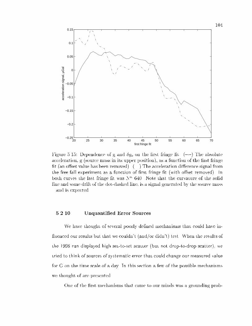
104

20 25 30 35 40 45 50 55 60 65 70−0.25

−0.2

−0.15

−0.1

−0.05

0

0.05

0.1

0.15

first fringe fit

acce

lera

tion

sign

al, µ

Gal

Figure 5.15: Dependence of g and �go on the �rst fringe �t. ({�{) The absoluteacceleration, g (source mass in its upper position), as a function of the �rst fringe�t (an o�set value has been removed). (|) The acceleration di�erence signal fromthe free-fall experiment as a function of �rst fringe �t (with o�set removed). Inboth curves the last fringe �t was No: 640. Note that the curvature of the solidline and some drift of the dot-dashed line, is a signal generated by the source mass{ and is expected.

5.2.10 Unquanti�ed Error Sources

We have thought of several poorly de�ned mechanisms that could have in-

uenced our results but that we couldn't (and/or didn't) test. When the results of

the 1998 run displayed high set-to-set scatter (but not drop-to-drop scatter), we

tried to think of sources of systematic error that could change our measured value

for G on the time scale of a day. In this section a few of the possible mechanisms

we thought of are presented.

One of the �rst mechanisms that came to our minds was a grounding prob-

105

lem between the experimental apparatus of the free-fall experiment and the FG-5.

Errors in the measurement of g as large as 10�Gal have been attributed by Micro-

g Solutions Inc. to unspeci�ed grounding errors, generally involving the super

spring system. The mechanism that would result in a mismeasurement of the

absolute acceleration is not clear.

There certainly were opportunities for ground loops to occur in our last

measurement. The drop initialization trigger was used in the airgap measuring

apparatus, in the FG-5 system, and in the shaft encoder output recording sys-

tem. The shaft encoder voltage was actually read by the FG-5 in place of the

super spring position. Additionally, the aluminum layer surrounding the drop-

ping chamber was held at 1.5 volts over a ground referenced to the chassis of a

power supply itself ground to the wall.

During the experiment, worried about such ground loops, I disconnected

the shaft encoder recording system for a quarter day, but didn't see any change

in drop-to-drop scatter. Since it was our set-to-set scatter that was surprising,

this really doesn't tell us much. Unfortunately the question of how ground loops

might a�ect the scatter is left unanswered. It is very di�cult to imagine a non-

pathological mechanism that would link any grounding problems to the source

mass position.

A second mechanism that could in uence low-frequency drifts in our exper-

iment was a random coupling of a higher order mode of the super spring to the

measurement. The super spring has a mode in which the spring that supports

the reference mirror twists. This mode has a frequency of approximately 0.3 Hz.

An amplitude of 7 �Gal would correspond to drop-to-drop scatter of 5 �Gal. The

decay constant of this mode is approximately 9 minutes. The twist mode is re-

sponsible for the majority of the g signal injected to the system by energy in the

super spring [47].

106

It is possible that the movements of the source mass maintained energy in the

twist mode without strongly changing its phase. Because a small vertical torque

is sensed by the oor when the source mass was moved, the excitation would by

systematic. Also, this would explain why the scatter in our G-values increased in

the data run of 1998, where there source mass was moved more frequently.

This mechanism is not very likely, however, because the amplitude of the

e�ect would be very small. The period of the torsion mode was observed to be

3.93 � 0.1 sec. At this frequency the worst case bias to the di�erence signal would

be 0.17 �Gal. The signal we saw in the data had a much larger amplitude than

this. The fact that no increased scatter was observed in the beginning of each set

as opposed to the end of the set (Section 5.3) seems to indicate that this wasn't an

important e�ect. Finally, the gravimeter has been run continuously throughout

the movement of the source mass. As soon as the source mass motion ended, the

scatter immediately returned to its value before the move.

Let us, nevertheless consider a pathological case in which the beat frequency

between the measurement rate (1/5 Hz) and the spring (the pendulum mode of

the spring was close to 1 Hz) were very low (less than 0.02 Hz). Then the bias

introduced by the spring would not be averaged out over many cycles in each set.

In the case that the beat was 0.015 Hz, the bias could easily be 0.4 �Gal , in one

set. Assuming the phase and amplitude were maintained, the next set would be

biased by -0.4�Gal .

Thus, in the special case that the frequency of measurement was very close

to a multiple of the spring frequency, the underlying signal could very well have

been caused by phase drifts in the spring. It would not require a phase modulation

on the time scale of the sets, but only on the scale of the drifts. The fact that the

coherence did not clearly extend between di�erent days of data10 provides some

10 Each morning I suspended the measurements and down loaded the previous day's data

107

support for this mechanism. Because the coherence was not completely continuous

within a day, however, this is not a strong statement.

Examination of the Figure 5.16 shows that a low (mHz) signal can be seen

in some averaged sets. The sets were averaged in a region where the coherent

signal in the di�erence data was clearly evident. This is consistent with the idea

that the spring mode was randomly phase locked with the experiment.

0 10 20 30 40 50 60 70 80 90−12

−10

−8

−6

−4

−2

0

2

4

6

Drop number

Acc

eler

atio

n, µ

Gal

Figure 5.16: Plot of acceleration value by drop averaged over 26 sets (13 withthe source mass down). Notice that there is an underlying signal in the datathat suggest the presence of systematic drifts linked to the start of each set. Thisunderlying systematic is consistent with the a random phase locking of the superspring torsion mode and the measurement cycle of the gravimeter.

from the gravimeter computer. Sometimes I allowed the source mass to continue its motions,because this seemed to reduce wear in the support nuts. Generally it took about an hour todown load the data and reinitialize the gravimeter.

108

5.3 Evidence of other Systematic Errors

Systematic errors that do not perfectly mimic parabolic motion would leave

telltale signatures in the record of the test mass motion. For this reason I hoped

to unearth evidence of systematics by looking for anomalous signals in the drop

data. I used a variety of methods, which are presented here.

Any dependence of G on the portion of the drop we analyzed is evidence

of a systematic error. This is related to the work in Secs. 4.3 and 5.2.1, where

the examination of the dependence of G on the �rst �t fringe (FFF) was used to

extract information about the position of the start of drop and the airgap signal.

Plots of the dependence of G on FFF for two data runs are shown in Figures 6.7

and 6.1.3. It is also possible to look for the dependence on the last fringe �t, as

in Figure 5.17, but it was more reasonable to analyze dependence on start fringe

than on end fringe because the start of the drop in uenced the �t for acceleration

much more strongly than the end. In fact the �rst half of the data accounts for

90% of the information about the acceleration. Also the source mass signal was

much more clear at the beginning of the drop than at the end.

Other signs of corrupting signals may be found by analyzing the g values

measured with the mass up, as opposed to the mass down. A di�erent amount of

drop-to-drop or set-to-set scatter could indicate a systematic e�ect. No signi�cant

di�erences were found. The drop-to-drop scatter was also compared between the

beginnings and ends of sets of data, and was identical, suggesting that there was

no appreciable excitation of the super spring during the movements of the source

mass. In Section 5.2.6 sets of data representing the average set with the source

mass either up or down were computed. The acceleration values of the nth drop

of every mass-up set were averaged together to give the value of the nth drop

of the average mass-up set. This was also done for the source mass in its lower

109

560 580 600 620 640 660

83

83.5

84

84.5

Last fringe fit

δg s

igna

l, µG

al

Figure 5.17: A comparison of delta g as a function of last fringe �t to theory. The�rst fringe �t was fringe 20. This data is extracted from a single day of data inthe 1998 data run. The plot with error bars and circles is the experimental curve,while the smooth line of stars represents theory. Note the small sinusoidal signalin the data. I attribute this to the oscillating airgap signal.

position. The averaged sets are shown in Figure 5.12. These sets would re ect

the presence of any systematic error parameter that would shift from one value to

another over the time of a single set. Thermal signals coupled to the source mass

position, for example, could slowly change the temperature of the ion pump, in

turn changing its e�ciency, the vacuum pressure, and the residual gas forces on

the test mass. No evidence of these drifts is seen in the averaged results. Figure

5.16 shows the set-average for a short segment of suspicious data. Less than 20

sets were averaged for this plot which does display drifts.

Another test for systematics involves using the only half the data: Comput-

ing the di�erences using just the second half of each set and comparing them to

the di�erences calculated using just the �rst half of each set would allow linear

drifts (in g, as a function of the time from the start of the sets) to be identi�ed.

Processing all the 1998 data in this way resulted in two values for G (one value

110

using the �rst half of set data, one value with the second half of set data). The

two values were consistent. The di�erence between them was (0.007 � 0.01) x

10�11 m3/kg-s2.

5.3.1 Residual Analysis

Valuable information remains in the residuals to each �t of drop data. Each

�t produces values for the parameters of the parabolic function Eqn. 2.10. By

subtracting the curve speci�ed by these parameters from the data, a set of residual

values is found, as in Fig. 5.18.

Information about various systematic errors may be extracted from these

residuals. In the method of Klopping [39] the set of decaying sinusoids is assumed

to describe many systematic errors in the measurement of g. Decaying sinusoidal

signals might arise from vibrations excited by the drop, as in Secs. 5.2.3 and

5.2.1. A damped sine wave apparent in the test mass motion would clearly not

result from any reasonable gravitational source.

Klopping developed a system that �t and removed decaying sinusoids from

the data. The frequencies of the sinusoids were found by spectral analysis of the

residuals to the drops, then the damping rate and amplitude were found with non-

linear �tting techniques. His method is cited by Micro-g Solutions as an accepted

provider of corrections for the airgap e�ect and is used to correct for di�erent oor

responses at absolute gravity sites.

We hoped to use Klopping's software to remove the airgap e�ect, and any

other unknown signals. I wrote a program that read in the frequencies and decay

constants11 of the four largest decaying sinusoids for each set of data and then used

11 The frequencies and decay constants were provided by a modi�ed version of the TREX.EXEsoftware that is standard to the FG-5 system. TREX.EXE is only con�gured for use with lowdata density data (180 data points per drop). The modi�cation allowed permitted use with ourhigh-density data (700 data points per drop)

111

0.02 0.04 0.06 0.08 0.1 0.12 0.14 0.16 0.18 0.2 0.22−4

−3

−2

−1

0

1

2

3x 10

−8

Time, seconds

Res

idua

ls, c

m

Figure 5.18: The residuals-to-drop averaged over 150,000 drops. The upper curveis the average residual, including data from both source mass positions. Thechoppy middle curve is the di�erence between the averaged residuals with thesource mass in its upper and lower positions (with o�set included). Note thatthe slight \M" shape of the di�erenced residuals is due to the higher order e�ectsof the source mass (as in Fig.2.2). The theoretical expectation for the di�erencein residuals is shown with the smooth curve overlying the di�erenced residuals.The lowest curve is the di�erenced residuals with the model removed (and o�setadded). Any signal visible in the lowest curve represents the trace of a systematicerror.

them to provide set corrections for the data. The set corrections would remove

the airgap e�ect from all the data and the airgap problem would be solved.

This method of attack was unsuccessful. The set corrections did not reduce

set-to-set scatter of g-values signi�cantly, suggesting that the corrections calcu-

lated by this analysis were not valid. Also the uncertainty in �go grew very large

112

due to the inclusion of many �tting parameters (a damped cosine and sine func-

tion for each decaying sinusoid; a total of 8 extra parameters) in the least-squares

�t. The lowest frequency of the sinusoids was 10 Hz | low enough to correlate

strongly with the cubic and quartic components of the perturbing signal (as in

Fig. 2.2, part B). This meant that the sinusoids would remove part of the source

mass signal as well as any airgap errors.

CHAPTER 6

DATA AND RESULTS

6.1 Data Runs

We used the free fall method in three data runs, presented here in chrono-

logical order. The �rst was a proof-of-concept experiment that I call the \bronze

mass run." The second acquired 9 days of data over a 13 day period in early May

1997. The third run incorporated several improvements to the apparatus and was

conducted in late May of 1998.

6.1.1 The Bronze Mass Experiment

In the summer of 1995 David Newell and Paul Keyser, both graduates of

JILA in physics, developed a system that allowed a bronze ring-shaped mass to be

placed above and far above an FG-5 free fall gravimeter. In this way a di�erential

measurement of the ring's gravity �eld could be made, but with only (at best) one

half the optimal signal-to-noise. The system was built in JILA and was su�cient

to show that the acceleration of gravity, as measured with a free fall gravimeter,

could be perturbed with an external source mass.

I modi�ed the apparatus in order to allow the source mass to be placed both

above and below the region of the drop. The modi�ed apparatus was portable,

and was setup at the Table Mountain Gravity Observatory (TMGO), a much

better (vibrationally quiet) site for gravity measurements than JILA. Figure 6.1

114

is a picture of the setup. This arrangement did not make provisions for high

accuracy positioning of the source mass.

The source mass of this run was made of two bronze rings that had been

used in two previous G experiments. The �rst experiment was that of Michael

Hulett, who in 1969 measured the de ection of a horizontal pendulum due the

gravitational attraction of the rings. His work was performed for his senior honors

thesis with James Faller.

The bronze masses were reused in a G experiment that used a magnetic

support system to escape the relatively sti� torsion constants of a �ber. This

experiment was conducted by William Koldewyn in the mid 1970s, again with

advisor Jim Faller [9]. Koldewyn had the masses precision machined and carefully

measured their volumes. We used his density values in our theoretical models

of the system. The two rings weighed approximately 100 Kg (combined), and

produced an acceleration signal of approximately � 10�Gal. We were very lucky

that the bronze rings were just large enough to �t over the vacuum chamber of

the gravimeter, but we were not able to get the mass low enough to reach its lower

optimal position | the rings were too tall.

The lifting arrangement relied upon a counterweight to balance the weight

of the source mass. The translation of the chain and counterweight meant that the

movement of the source mass could not be treated simply as a translation of the

perturbing acceleration �eld about the start-of-drop position. This complication,

coupled with an ugly system of bearings, hangers, and plates, made the mass

arrangement di�cult to model accurately.

The FG-5 gravimeter we used had a standard (at the time) data acquisition

system that was only capable of recording 180 position-time pairs for each drop of

the proof mass. Nevertheless the drop-to-drop scatter in the data was not much

worse than the best data we would ever take (only about 20% greater scatter). A

115

Figure 6.1: A photo of the source mass and a portion of the lifting assembly ofthe bronze proof-of-concept experiment. Note that the mass is made only twocylinders. It was supported by a chain, and was guided by three rods.

116

sample of the data is plotted in Figure 6.2. This data acquisition system had some

other disagreeable properties. There was a delay of approximately 30 milliseconds

between the start of the drop and the start of data acquisition. This was due

to the time required for the system to initialize after receiving the trigger signal

indicating the start of the drop. Thus the fringes recorded by the system were not

well connected to the position of the start of the drop. The system could not keep

up with the fringe data from the interferometer, and would miss fringes towards

the end of the drop.

Because our software implementation of the theoretical system was not com-

pleted at the time of the bronze mass experiment the source mass was not correctly

placed in its optimal positions. The data from this run were taken with a variety

of upper and lower source mass positions, including some scans where the source

mass was slowly stepped through its range.

All in all the bronze mass run was a valuable learning experience but not

much more. Figure 6.3 shows a plot of the results of this �rst data run. The

results are clearly \in the ball park" of the correct value of G, though they are

also only of proof-of-concept quality.

The bronze mass experiment illustrated the need for a robust system with

improved signal-to-noise and a simpler mass arrangement (for modeling). During

1996 we worked on the completion of the software system as well as the design

and construction of the apparatus to be used in the actual measurement.

117

0 2 4 6 8 10 12−40

−30

−20

−10

0

10

20

30

40

Time, hours

Acceleration,�Gal

Figure 6.2: A 13 hour sample of acceleration data from the bronze proof-of-conceptexperiment. Note that the signal of the bronze ring source mass has an amplitudeof only 10 �Gal.

0 2 4 6 8 10 12 14 16 18 206.4

6.5

6.6

6.7

6.8

6.9

7

Day number

G X

1011 ,

m3 /k

g−s

2

Figure 6.3: Results of the bronze mass proof-of-concept experiment. The valuemarked with an asterisk represents the �nal value of the data run. For comparison,the accepted value of G is 6.6726 � 0.0009 X 10�11 m3/kg-s2.

118

6.1.2 May 1997 Experiment

The May 1997 experiment used the lifting assembly and apparatus described

in Chapter 3. By this point we had developed a sophisticated software system to

calculate the proper source mass positions and to analyze data. The gravimeter

was equipped with a new data acquisition system that allowed four times denser

data than could be recorded previously. This was expected to reduce the drop to

drop scatter of acceleration measurements by close to a factor of two (sqrt(4) = 2).

The high-speed data acquisition system solved the problems with missed

fringes late in the drop and the uncertainty in the delay between the start of drop

and the start of data acquisition. There was still a delay for the fringe signal

frequency to rise past 700 Hz (where it could trigger the discriminator) but this

was a negligible error source (a fringe signal above 700 Hz is achieved in just a

few microns of vertical displacement).

The nine days of data that we took (over a 13 day period) gave the results

shown in Figs. 6.4 and 6.5. In order to compare the internal and external scatter

of the data I averaged individual di�erences in a variety of bin sizes. With a bin

size of 20, 30, 50, and 81 the external scatter was 1.5, 1.3, 1.6 and 1.3 times as

large as the internal. Averaging these results indicates that a reasonable ratio is

1.4; there is more variation in the G value from bin to bin than would be expected

from the scatter within each bin.

The di�erence values (Fig.6.6) produce a power spectrum that is at, how-

ever, suggesting that there was no unusual power at low frequency (that could

strongly bias our result). The lack of a clear drift over the whole data set sup-

ported this assumption. Fitting the individual di�erence with a line gave a drift

in �go equivalent to 0.20 � 0.13 �Gal from the start of the data run to the end

(13 days). The drift estimate is suggestive, but not clearly indicative of a drift.

119

The reduced chi-squared comparison of the daily results to a Gaussian (as

presented in [48, 49]) returned ~�2 = 0:8 (40% probability). This indicates good

agreement with a Gaussian. Calculating the reduced chi-squared from the indi-

vidual di�erences, however, returns a value of ~�2 � 3 (10% probability).

These results do not damn the 1997 data run, but they do suggest the

presence of either a random coupling of environmental signals to the G-experiment,

or the random modulation of an unknown systematic. Because the experiment

was run during a hot spell in Colorado we attributed the low-frequency scatter to

air conditioning cycles correlating with the experiment. The air conditioning at

the site was observed to switch on and o� at slightly higher frequencies than the

source mass was modulated.

An estimate of the bias introduced by the underlying signal could be made

by modeling it as a sinusoid in the data and calculating the o�set introduced

by a fractional period. Alternately an estimate of the e�ect could be made by

selectively removing bins of data, and recording the e�ect on the mean. These

two methods returned estimates of the bias that agreed to 10%. Using the second

method, we adopted an estimate of 450 ppm for the random drift bias error in

the 1997 result.

The �nal result of the 1997 was calculated in a more complicated way than

by simply averaging di�erences. Instead G was calculated as a function of the �rst

fringe �t (FFF) from the �go curve found in Section 4.3. Figure 6.7 is a plot of

this curve. The value of the constant produced by the data depends on the choice

of the �rst fringe �t. I characterize this dependence as weak because the standard

deviation of the values computed with di�erent FFFs is 1/3 of the uncertainty

of each result with a single choice of FFF. A component of the \noise" between

the di�erent start fringes was due to the fact that we extract G from a slightly

di�erent sets of data for each value.

120

A0 50 100 150 200 250 300 350 400 450 500 550

79

80

81

82

83

84

85

Difference number

Diffe

renc

e sig

nal,

µGal

B79 80 81 82 83 84 85

0

5

10

15

20

25

30

35

40

45

δ g value, µGal

Cou

nt

Figure 6.4: Data from the 1997 experiment. A) Di�erences as measured in Sec4.2.1. The dotted line represents the individual di�erences, while the solid line isthe di�erence value averaged over blocks of 20 individual values. B) Histogram ofthe di�erences. The solid line is the best �t Gaussian curve.

121

130 132 134 136 138 140 142

6.66

6.67

6.68

6.69

6.7

6.71

6.72

G X

1011

m3 /k

g−s2

Day

Figure 6.5: Results of the May 1997 experiment. Daily results. The value markedwith an asterisk represents the �nal value of the data run. The error bars representa single standard error, only. The lowest horizontal line represents the 1995 NewZealand result [15], the middle line is the accepted value [4], and the upper lineis the 1995 German result [14].

122

A)0 0.1 0.2 0.3 0.4 0.5 0.6 0.7 0.8 0.9 1

−20

−15

−10

−5

0

5

10

Frequency

Powe

r Spe

ctrum

Mag

nitud

e (dB

)

B) 0 50 100 150 200 250 300 350 400 450 500 55081.5

81.6

81.7

81.8

81.9

82

82.1

82.2

82.3

82.4

Difference number

Accele

ration,

µGal

C)0 0.1 0.2 0.3 0.4 0.5 0.6 0.7 0.8 0.9 1

−35

−30

−25

−20

−15

−10

−5

Frequency

Powe

r Spe

ctrum

Mag

nitud

e (dB

)

Figure 6.6: Power spectral analysis of individual di�erences from the 1997 ex-periment. A)The power spectrum from di�erences calculated using method two(of Sec 4.2.1). Only half of the di�erences were used in the calculation to avoidany correlation between the individual values. B)The di�erence values averagedin groups of 20. This corresponds to periods of approximately 7 hours. C) Thepower spectrum of the binned data. The power spectrum with bins of 3.5 hourslooks much same, with just a bit more de�nition.

123

The variation in the value raises the question of which value is appropriate

to summarize the result. Because we don't expect that G be physically dependent

on the FFF, a �t of all this data to a at line gives a reasonable indicator (the

weighted mean value) for our best estimate for G.

Some portion of the dependence of the measured G on the FFF was system-

atic. The data points in Fig. 6.7 are not completely independent, as is especially

obvious between fringes 24{30 and beyond fringe 60. An estimate of the sensitivity

of our \best value" to possible systematics in the data can be made by calculating

the change in the value when di�erent portions of the curve are excluded from the

calculation of the mean (this assumes that there is no signi�cant DC systematic

bias). Figure 6.8 is a plot of the error estimate in G as a function of start fringe.

The two \especially suspicious" regions between fringes 24{30 and 60 onwards are

marked. The mean value is very insensitive to the G-values in these regions, in

part because of their larger uncertainties. The weighted mean value shifts only

1/10th of a standard uncertainty when these data points are excluded. The point

that the exclusion of this data may be considered arbitrary is moot because our

results are insensitive to this manipulation.

The value of G extracted from the 1997 run is the weighted mean of the

data shown in Figure 6.7 with a statistical uncertainty of 450 ppm. The statistical

uncertainty was based on the complete data set evaluated from fringe 20 to 640 (a

region chosen for its compatibility with absolute gravity measurements). The error

bar includes estimates of error sources as discussed in Section 5.2 and Appendix

B. The 1997 result is:

G = (6:6863� 0:0015� 0:0042� 10�11m3=kg� s2

where the �rst uncertainty estimate is the root sum square of the systematic

errors of Table 5.1 and the second uncertainty is the random error associated with

124

A.20 40 60 80 100 120 140 160

6.675

6.68

6.685

6.69

6.695

6.7

Start fringe

G X

1011

m3 /k

g−s2

B.20 40 60 80 100 120 140 160

6.681

6.682

6.683

6.684

6.685

6.686

6.687

6.688

6.689

6.69

Start fringe

G X

1011

m3 /k

g−s2

Figure 6.7: G as a function of �rst fringe �t to a �xed �nal fringe (#640). A)With error bars associated with the analysis of the complete 1997 data set witheach particular choice of �rst �t fringe. B) Without error bars.

125

A.0 20 40 60 80 100 120 140 160

3.5

4

4.5

5

5.5

6

6.5

7

7.5

8x 10

−3

Start fringe

Err

or e

sim

ate

(m3 /k

g−s2 X

1011

)

B.0 20 40 60 80 100 120 140 160

6.681

6.682

6.683

6.684

6.685

6.686

6.687

6.688

6.689

6.69

6.691

Start fringe

G (

m3 /k

g−s2 X

1011

)

Figure 6.8: Statistical uncertainty in G as a function of �rst fringe �t to a �xed�nal fringe (#640). A) The error estimates plotted against start fringe. Thevertical lines are at fringes 24, 30, and 60. B) Error (|) scaled for comparison tothe actual G values ({�{) error.

126

a bias in the data from the underlying signal and the statistical uncertainty. The

combined statistical and systematic error estimate is 0.0045 x 10�11 m3/kg-s2 (670

ppm).

127

6.1.3 May 1998 Experiment

We made several improvements to the apparatus for the 1998 data run.

Concerned about thermal signals we added a layer of insulation (Cryotex) around

the whole lifting assembly and a separate loose thermal shield for the laser and

electronics system of the gravimeter. We increased the frequency of modulation

of the source mass position by nearly a factor of two, decreasing the correlation

of random environmental signals and machine drifts to the G measurement.

One way temperature signals could in uence the scatter in the free fall ex-

periment was by causing tilts of the laser verticality (see Section 5.2.4). For

this reason we used a �ber-optic interferometer system that had shown improved

verticality stability over the standard FG-5 interferometer(see Sec. 3.1.3 for dis-

cussion).

We directly measured the motion of the air-vacuum interface throughout

the experiment. We hoped that this auxiliary data would help us to place bounds

on the di�erential airgap signal (Section 5.2.1). In addition to airgap data we

logged the shaft-encoder voltage (Sec. 3.1.1.2) and ion-pump voltage1 for each

drop.

We attempted to increase the precision of the experiment by using a super

spring that had demonstrated superior performance, and by doubling the dropping

rate from a drop every 10 seconds to one every 5 seconds.

We made several \miscellaneous" changes. To remove the magnetic signal of

the drive motor (Section 5.2.8) and reduce magnetic damping of the airgap motion

(Section 5.2.1) magnetic shielding was placed around the motor and ion pump.

To improve the performance of the lifting assembly and decrease deformation of

the source mass the support plates (Section 3.2) were replaced with thicker plates

1 The ion pump voltage gave a crude estimate of the vacuum pressure in the droppingchamber.

128

with extra support rods.

Figures 6.9 and 6.10 show the results of these improvements. The scatter in

set-to-set g values increased by a factor of 1.9. The the scatter in �go increased by

a factor of 1.5. The increase in scatter was not seen at the high frequency of drop

measurements, but only in set-to-set scatter. The ratio of internal to external

scatter increased to 1.9. The value of G extracted from this data, however, was

consistent with the 1997 value. We don't know what caused this unexpected

increase in scatter.

There was some coherence between the individual �g di�erences, as in Fig-

ure 6.10. The histogram of the whole set of data, however, displays a normal

distribution (Table 6.1 gives the major moments of the distribution, with \typ-

ical" values for the kurtosis and skew), and the power spectrum (Fig. 6.11) is

reasonably at. This suggests that the correlations are random. A �t of a line to

the data gives a drift value corresponding to a change of 0.065 � 0.10�Gal from

the beginning to the end of the data set (15 days). Assuming that the signal was

random, a bias error estimate of 0.004 x 10�11 m3/kg-s2 (600 ppm) was adopted.

This was calculated in the same way as in the 1997 data run.

Moment Value TypicalMean 82.8633 �GalAverage Deviation 0.90 �GalStandard Deviation 1.16 �GalVariance 1.34 �Gal2

Skewness 0.12 0.1Kurtosis 0.34 0.24

Table 6.1: Main moments of the 1998 experiment distribution of �g observations.The values for the kurtosis and skew are close enough to \typical" values to beconsidered normal.

The 1998 data displays much the same scatter in G as a function of �rst

fringe �t as the 1997 data (Figure 6.1.3). It, too, displays coherence between

129

A.138 140 142 144 146 148 150 152 154 156

6.62

6.64

6.66

6.68

6.7

6.72

6.74

6.76

Day

G X

1011

, m3 /K

g−s2

B.78 79 80 81 82 83 84 85 86 87 88

0

50

100

150

200

250

δ g value, µGal

Cou

nt

Figure 6.9: Results of the 1998 data run. A) Daily results. The horizontal linesrepresent values for G from other recent experiments: The upper line is the PTBresult, the middle line is the accepted NBS result, and the low line is the NewZealand Standards result. The daily results re ect the coherence obvious in Fig.6.10. B) A histogram of the individual 1998 �g di�erences. The smooth curvesrepresent the normal probability for the mean and variance of this data. Thelarger curve consists of 1660 points in 30 bins, while the lower curve is the samedata in 70 bins.

130

A.0 200 400 600 800 1000 1200 1400

78

80

82

84

86

88

Diff

eren

ce s

igna

l, µG

al

Difference number

B.0 200 400 600 800 1000 1200 1400 1600 1800

81.5

82

82.5

83

83.5

84

84.5

Difference number

Diff

eren

ce s

igna

l, µG

al

Figure 6.10: Individual di�erences from the 1998 data run. A) The di�erences,calculated using method 3 of Sec. 4.2.1. B) The di�erences averaged in bins ofwidth 40. The dotted line is a running average, while the solid line is simplybinned data.

131

A)0 0.1 0.2 0.3 0.4 0.5 0.6 0.7 0.8 0.9 1

−6

−4

−2

0

2

4

6

8

10

12

Frequency

Powe

r Spe

ctrum

Mag

nitud

e (dB

)

B) 0 200 400 600 800 1000 1200 1400 1600−2

−1.5

−1

−0.5

0

0.5

1

1.5

Binned difference values

Accel

eration

, µGal

C)0 0.1 0.2 0.3 0.4 0.5 0.6 0.7 0.8 0.9 1

−25

−20

−15

−10

−5

0

5

Frequency

Powe

r Spe

ctrum

Mag

nitud

e (dB

)

Figure 6.11: Power spectral analysis of the individual di�erences from the 1998experiment. A) The power spectrum from di�erences calculated using method 2of Sec. 4.2.1, but only every other value was used in the power spectrum to avoidcorrelated data at the higher frequencies. B) The di�erence data was placed intobins representing 3.6 hour periods. C) The power spectrum of the binned data.

132

the values. Once again the weighted mean value of G given by these results is

insensitive to exclusion of suspicious data, changing by less than 1/10th sigma

when the data is removed. The weighted mean of this data (associated with 700

ppm statistical uncertainty and adjusted with the airgap correction) forms the

1998 data run result:

G = (6:6896� 0:0013� 0:0062)� 10�11m3=kg� s2

where the �rst uncertainty is root sum square of the systematic errors of Table 5.1

and the second uncertainty is the RMS error associated with a bias in the data

from the underlying signal and the statistical variation of the data. The combined

statistical and systematic error estimate is 0.0063 x 10�11 m3/kg-s2 (940 ppm).

6.2 Combined Results

The large underlying signal in the 1998 data could represent a randomly

modulated systematic error. If this was the case there could be a systematic bias

that we would not be able to identify in the data. Consider the hypothetical

situation that our assessment of the thermal coupling between the source mass

and gravimeter was vastly underestimated. Clearly the coupling would not exist if

all components of the gravimeter and the source mass were the same temperature.

If there was a �xed o�set in the source mass temperature, however, a constant bias

to the �g signal would occur. And if the source mass temperature had a constant

o�set with a random time varying component data such as we've seen might have

resulted. It is not clear that there was such an o�set, but to be properly cautious,

we must deal with this possibility.

The only information that we have that there is no low frequency or DC

bias in our results is the agreement between our two data runs. The fact that

they were not completely independent is unimportant because the scale of known

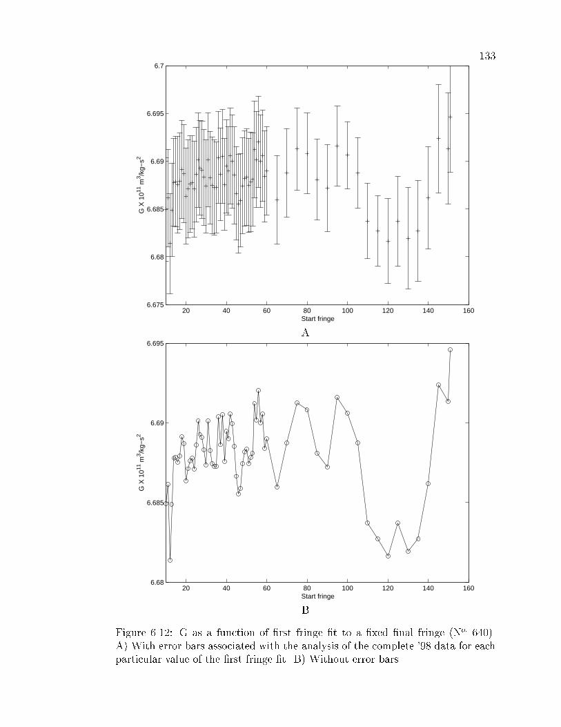
133

20 40 60 80 100 120 140 1606.675

6.68

6.685

6.69

6.695

6.7

Start fringe

G X

1011

m3 /k

g−s2

A

20 40 60 80 100 120 140 1606.68

6.685

6.69

6.695

Start fringe

G X

1011

m3 /k

g−s2

B

Figure 6.12: G as a function of �rst fringe �t to a �xed �nal fringe (No: 640).A) With error bars associated with the analysis of the complete '98 data for eachparticular value of the �rst fringe �t. B) Without error bars.

134

systematic errors is very small compared to statistical and possible systematic

uncertainties. We can make an estimate of our uncertainty arising from such a

low-frequency bias by taking the di�erence of the two runs. This di�erence is only

400 ppm (the two results don't di�er in a statistically signi�cant way), but the

uncertainty in the di�erence is 1100 ppm (0.11%).

For the �nal result of the free fall experiment we combine the 1997 and

1998 data runs. The two experiments were not fully independent; they used the

same tungsten masses arranged in roughly the same orientations. Therefore the

correct combined error of the two data runs is slightly larger than the uncertainty

in the mean of the combination. Adopting the uncertainty in the di�erence as

an estimate of a possible underlying systematic o�set increases the uncertainty in

the mean to a level were these distinctions are unimportant.

The combined �nal result for the free fall experiment is:

G = (6:6873� 0:0076) � 10�11 m3=kg � sec2:

The uncertainty corresponds to 1150 ppm, 0.12%. This result is shown with all

the daily results and some other recent results in Figure 6.13. This value for the

constant lies 1.5 standard errors above the accepted value, and 3 standard errors

below the German PTB result. Although this result does not uphold the PTB

value at all, it does lend some support to the region above the accepted value.

135

6.62

6.64

6.66

6.68

6.7

6.72

6.74

6.76

1

2

3

4

5

G X

1011

m3 /k

g−s2

1997 Results 1998 Results Recent Results

Figure 6.13: A plot of G results. At the right side of the �gure, recent results: 1.NBS. 2. New Zealand Standards. 3. PTB. 4. Wuppertal. 5. Z�urich. The �nal freefall result is the value marked with a circle, and includes all error estimates. Theother results marked with crosses are the daily results of the free fall experiments.The error bars of the daily results represent statistical uncertainty, only. Theweighted mean result of each data run is marked with an asterisk. These valuesinclude the error estimates of Table 5.1, statistical uncertainty, and the estimateof bias errors from the underlying signals.

CHAPTER 7

CONCLUSION

The free fall determination of G is conceptually simple. An idealized model

describing the motion of a falling mass has been well understood for literally

hundreds of years. The study of objects moving in gravitational �elds begins at

the start of an education in physics.

Yet somehow G measurements are full of complexity, subtlety, and beauty

| and the free fall experiment is no exception. The complexity of the experiment

arises from the fact that our measurement pushes on the boundary between the

idealized model and the hard reality of measurement. The calculation of the

mutual attraction of the source mass and the proof mass involved over 6000 six-

dimensional integrals calculated at 1000 positions along the drop range of the test

mass.

The subtleties of the experiment are found mostly in the search for system-

atic errors. The source mass in uences the resonances of the lifting assembly in

di�erent ways, depending on its position. These resonances, which extend to be-

low 70 Hz, a�ect the response of the oor to the changing weight of the dropping

system. The weight changes because portions of the dropping chamber (the co-

falling chamber and the proof mass) become weightless during the drop. Thus the

change in source mass position a�ects the airgap measurement (Section 5.2.1).

The beauty of the free fall method lies in the hints of simplicity that remain

137

in the experiment. The fact that the sensing mass of the experiment is unsup-

ported means that dependencies on material properties are greatly reduced if not

completely removed. The fact that the measurement is di�erential means that

common mode errors of gigantic magnitudes can be tolerated. The modulation

rate of the source mass pushes the gravity signature of the source masses beyond

the frequencies of most environmental signals.

7.1 Results

Our �nal value for G is

G = (6:6873� 0:0076) � 10�11 m3=kg � sec2:

This result incorporates error estimates of random drift bias errors and an estimate

of a DC shift between the results of the two data runs. This was not the ideal

situation, as made clear by Churchill Eisenhart:

I realize that some of the subjectively estimated uncertainties tab-ulated by experimenters are intended, when combined \in quadra-ture" with the statistical standard error of the mean, to provide anin ated \standard error" of the mean that can be used to \providean indication of how closely the result of this experiment is likelyto agree with other results that might be obtained if the entireexperiment were carried out afresh `from the beginning,' " butexperience shows that this is a delusion: there is no substitutefor comprehensive realistic repetitions of the entire experiment!|Churchill Eisenhart [50]

It is unfortunate that the gravimeter system was not available for in depth

testing with the source mass system, or for additional experimental runs. In some

sense it was this lack of time with the gravimeter that was our greatest nemesis.

It was for this reason that we had to adopt the di�erence in the results of the

1997 and 1998 data runs as an estimate of systematic bias errors. This estimate

138

is not unreasonable:

The uncertainty assigned to a precision measurement ideally shouldnot be solely determined by random measurement errors, butshould partly be the result of subjective judgments by the ex-perimenter on the accuracy of his work." | Abstract by PeterFranken [51]

7.2 Future

At the time that we did our experiments it was not quite clear to what

precision we would be able to extend the performance of the FG-5. Now, with

the lifting assembly packed away and the tungsten masses waiting for their next

leading role, I believe I can clearly see the future of the free fall method.

There are only two ways in which the free fall experiment will be contin-

ued. In a series of small improvements, or in a single big step. The combined

uncertainty of our results is 1300 ppm, the systematic errors arising from mass

homogeneities, modeling errors, and positioning (internal to the source mass) only

rear their ugly heads at the level of 100 ppms. Clearly our results can be improved

dramatically if the sources of the underlying drifts could be identi�ed and con-

trolled.

If the random signal were removed from our data and questions of low-

frequency biases were laid to rest then a result at the level of 300 ppm could be

achieved with the present system. Clearly our data would be close to this level if

not for the underlying signals.

I have thought of several lines of attack that might be used to track down

the drift source. For example, \double moving" the source mass in between sets

might give information about spring e�ects. After each set of data the source mass

would be moved half way to its alternate position, and then immediately moved

back to its original position. Increased scatter in this situation would indicate

139

that the move was linked to the noise source.

Once the source of the drift was identi�ed, however, and a measurement at

the level of 300 ppm completed, further improvement of more than a factor of

two would be very di�cult to achieve. In this context many of the improvement

ideas that I entertained are simply not worth the e�ort. The \return" on small

improvements to the system would not be worth the investment. A dramatic

scale-up of the system would be more interesting.

A large scale-up of the experiment would involve a large increase in the

time, money and energy spent on the determination. The experiment would be

performed in its ideal incarnation, incorporating many ideas independently of

the constraints of weight and portability that in uenced the current gravimeter

system.

The entire dropping assembly would be custom designed to operate at a

single location. It would include a simpli�ed proof mass less sensitive to eddy

currents, and counterweighted to reduce vibration. The position of the test mass

would be recorded at every fringe crossing, not each 500th. The interferometer

system would be used to reference the start-of-drop position to the source mass.

External magnetic �elds would be removed either with shielding or active control.

The vacuum pump could be moved far away from the rest of the system. The

laser would be, for example, a frequency doubled Nd:YAG green laser. This type

of laser can be stabilized to better stability than the HeNe, without the large

frequency dither of the current system.

The source mass would be located in the same evacuated room1 as the

test mass. The source mass would be made not of just twelve tungsten billets,

but of hundreds of smaller precision machined objects placed as close to the drop

as possible. They would be supported by a system capable of switching their

1 Including thermal isolation, naturally. A Big Step!

140

positions after every drop.

A custom super spring would be made for the experiment. Perhaps an multi-

dimensional active isolation unit as have been developed for use in gravity wave

detectors could be incorporated into its design [52]. The spring could be located

far from the dropping system (perhaps in the same vacuum) to reduce coupling

of oor motions.

It is certainly reasonable to wonder whether such a costly experiment using

the free fall method will ever be carried out. The free fall measurement currently

su�ers from lower signal-to-noise ratio than some other comparable experiments.

It also also has exhibited unexplained drifts. But the great characteristic of the

method is its use of an unsupported mass in a system that, in theory, is extremely

simple.

There are several G-experiments that are expected to produce results by the

end of this year. If their results are consistent, and the value of G can be stated

with con�dence and precision, then I don't believe there is a strong future for the

free fall method. If the results continue to show great deviation in G, however,

then I believe that the conceptual simplicity of the free fall method, coupled with

its lack of dependence on material properties, will provide reasonable impetus for

an improved experiment.

I know what must be done to solve the problems inherent in the measure-

ment of G. Intelligent thought, unrelenting e�ort, big money, and a dose of luck

must be pooled for one carefully planned, constructed, and executed measure-

ment. I hope that the work presented in this thesis will help future experimenters

(as it helped me) to grasp the challenge of the measurement of G, and to recognize

some of the possible pitfalls in that measurement.

BIBLIOGRAPHY

[1] R. Wagoner, W. Fowler, and F. Hoyle Astrophysics Journal, vol. 148, 1967.

[2] H. Cavendish, \Experiments to determine the density of the Earth," Phil.Trans. R. Soc. London, vol. 88, pp. 469{526, 1798.

[3] R. Heyl. Res. Nat. Bur. Stand. (US), 1930. pg. 1243-1290.

[4] G. G. Luther and W. R. Towler, \Redetermination of the Newtonian gravi-tational constant, G," Physical Review Letters, vol. 48, no. 3, pp. 121{123,1982.

[5] M. Sagitov, V. Milykov, Y. A. Monakhov, V. Nazarenko, and K. G. Tadzhiki-nov, \A new determination of the cavendish gravitational constant," Dokl.Akad. Nauk. SSSR Earth Sci., vol. 245, pp. 20{22, 1981.

[6] O. Karagioz, V. Izmaylov, N. Agafonov, E. Kocheryan, and Y. Tarakanov,\The determination of the gravitational constant with an evacuated tor-sion balance," Izvestiya Akademii Nauk SSSR, Fizika Zemli, vol. 12, no. 5,pp. 106{111, 1976.

[7] G. T. Gillies, \The Newtonian gravitational constant: Recent measurementsand related studies," Rep. Prog. Phys., vol. 60, pp. 151{225, 1997.

[8] C. H. Bagley, A Determination of the Newtonian Constant of Gravity Usingthe Method of Heyl. PhD thesis, University of Colorado, Boulder, Colorado,1996.

[9] W. A. Koldewyn, A New Method for Measuring the Newtonian GravitationalConstant, G. PhD thesis, Wesleyan University, Middletown, Connecticut,1976.

[10] K. Kuroda, \Does the time of swing method give a correct value of the New-tonian Gravitational constant?," Physical Review Letters, vol. 75, pp. 2796{2798, October 1995.

142

[11] R. Newman and M. K. Bantel, \Preparation for a determination of g using acryogenic torsion pendulum," Proceedings of the Eighth Marcel GrossmannMeeting on General Relativity, June 1997.

[12] S. Matsumura, N. Kanda, T. Tomaru, H. Ishizuka, and K. Kuroda, \A mea-surement of the frequency dependence of the spring constant," Physics LettersA, vol. 244, pp. 4{8, July 1998.

[13] M. K. Bantel and R. D. Newman, \Measuremnet of torsion �ber anelasticproperties in preparation for a new measurement of g," Proceedings of the1998 Conference on Precision Electromagetic Measurement, 1998.

[14] W. Michaelis, H. Haars, and R. Augustin, \A new precise determination ofNewton's gravitational constant," Metrologia, vol. 32, pp. 267{276, 1995/96.

[15] M. P. Fitzgerald and T. R. Armstrong, \Newton's gravitational constant withuncertainty less than 100 ppm," IEEE Transactions on Instrumentation andMeasurement, vol. 44, no. 2, pp. 494{497, 1995.

[16] A. Schumacher, U. Kleinevo�, H. Sch�utt, et al., \Determination of the gravi-tational constant G using a Fabry-P�erot pendulum resonator," Proceedings ofthe 1998 Conference on Precision Electromagnetic Measurement, July 1998.

[17] J. Schurr, F. Nolting, and W. K�undig, \Gravitational constant measured bymeans of a beam balance," Physical Review Letters, vol. 80, pp. 1142{1145,Febuary 1998.

[18] H. Walesch, H. Meyer, H. Piel, and J. Schurr, \The gravitational force atmass separations from 0.6m to 2.1m and the precise measurement of G,"IEEE Transactions on Instrumentation and Measurement, vol. 44, pp. 491{493, 1995.

[19] H. Walesch, H. Meyer, H. Piel, and J. Schurr, \Determination of the gravita-tional constant G using a Fabry-P�ereot pendulum resonator." Available viaInternet at: http://wpos6.physik.uni-wuppertal.de:8080/ gravi.

[20] H. de Boer, H. Haars, and W. Michaelis, \A new experiment for the deter-mination of the Newtonian gravitational constant," Metrologia, 1987.

[21] F. Nolting, J. Schurr, and W. K�undig, \Determination of G by meansof a beam balance," Proceedings of the 1998 Conference on PrecisionElectromagnetic Measurements, July 1998.

[22] J. E. Faller, An Absolute Interferometric Determination of the Accelerationof Gravity. PhD thesis, Princeton, 1963.

[23] R. L. R. III, Super Spring | A New Type of Low-Frequency VibrationIsolator. PhD thesis, University of Colorado, Boulder, Colorado, 1983.

143

[24] T. M. Niebauer, New Absolute Gravity Instruments for Physics andGeophysics. PhD thesis, University of Colorado, Boulder, Colorado, 1987.

[25] D. S. Robertson, \Treating absolute gravity data as a spacecraft trackingproblem," Metrologia, vol. 33, pp. 545{548, 1996.

[26] D. Brouwer and G. Clemence, Methods of Celestial Mechanics. New York:Academic Press, 1961.

[27] W. H. Press, S. A. Teukolsky, W. T. Vetterling, and B. P. Flannery, NumericalRecipes in C. Cambridge University Press, second ed., 1992.

[28] W. H. Press, S. A. Teukolsky, W. T. Vetterling, and B. P. Flannery, \Nu-merical recipies routines and examples in c." Diskette, 1992.

[29] M. Winters, Model 100 Iodine-Stabilized HeNe Laser, Operator's Manual.Winters Electro-Optics, Inc., �rst ed., 1994.

[30] M. A. Zumberge, A Portable Apparatus for Absolute Measurements of theEarth's Gravity. PhD thesis, University of Colorado, Boulder, Colorado,1981.

[31] W. A. Koldewyn, A New Method for Measuring the Newtonian GravitationalConstant, G. PhD thesis, Wesleyan University, Middletown, Connecticut,1976.

[32] R. S. Davis, \Determining the magnetic properties of 1 kg mass standards,"Journal of Research of the National Insitute of Standards and Technology,vol. 100, pp. 209{225, 1995.

[33] R. S. Davis, 1997. Personal Communication to J. Faller.

[34] L. Mansinha, \Barometric and gravimetric observations of the 1999 solareclipse in europe," Proceedings of the 1997 AGU Chapman Conference onMicrogal Gravimetry, 1997.

[35] R. Warburton and J. Goodkind, \Detailed gravity-tide spectrum between oneand four cycles per day," The Geophysical Journal of the Royal AstronomicalSociety, vol. 52, no. 1, pp. 117{136, 1978.

[36] D. S. Robertson, G. Sasagawa, T. M. Niebauer, F. W. Klopping, J. E. Faller,and J. P. Schwarz, \Using spacecraft tracking algorithms to process absolutegravity data," German Geodetic Commission, row B, 1997.

[37] B. Putney, J. Brownd, and R. Gomez, Recursive Partitioned INversion ofLarge(1500 X 1500) Symmetric Matrices. Greenbelt, MD: NASA GSFC X-921-76-160, 1976.

144

[38] T. M. Niebauer, G. S. Sasagawa, J. E. Faller, R. Hilt, and F. Klopping, \Anew generation of absolute gravimeters," Metrologia, vol. 32, pp. 159{180,1995.

[39] F. Klopping, G. Peter, B. S. Robertson, K. Berstis, R. Moose, andW. E. Carter, \Improvements in absolute gravity observations," Journal ofGeophysical Research, vol. 96, pp. 8295{8303, May 1991.

[40] Micro-g Solutions FG-5 Owner's Manual.

[41] J. Faller and P. Keyser. Research and development of an opto-electric bubblelevel, JILA.

[42] Personal communication with Jim Faller.

[43] D. J. Summner and A. K. Thakkrar, \Experiments with a 'jumping ring'apparatus," Physics Education, vol. 7, pp. 238{242, 1972.

[44] J. Hall, \Forces on the jumping ring," The Physics Teacher, vol. 35, pp. 80{83, Feb 1997.

[45] W. M. Saslow, \Electromechanical implications of Faraday's law: A problemcollection," American Journal of Physcis, vol. 55, pp. 986{993, November1987.

[46] J. Faller, W. Hollander, P. Nelson, and M. McHugh, \Gyroscope-weighing ex-periment with a null result," Physical Review Letters, vol. 64, no. 8, pp. 825{6, 1990.

[47] Personal Communication with Fred Klopping, September 1998.

[48] J. R. Taylor, An Introduction to Error Analysis, The Study of Uncertaintiesin Physical Measurements. Mill Valley, CA: University Science Books, 1982.

[49] P. R. Bebington and D. K. Robinson, Data Reduction and Error Analysis forthe Physical Sciences. McGraw-Hill Inc., second ed., 1992.

[50] C. Eisenhart, \Contribution to panel discussion on adjustmenets of the fun-damental constants," in NBS Special Publication 343. Precision Measurementand Fundamental Constants (D. Langenburg and B. N. Taylor, eds.), Pro-ceedings of the International Conference held at the National Bureau of Stan-dards, (Gainsburg, MD), pp. 509{517, Aug 1970.

[51] P. Franken, \Comments on the assignements of experimental uncertainties,"in NBS Special Publication 343. Precision Measurement and FundamentalConstants (D. Langenburg and B. N. Taylor, eds.), Proceedings of the Inter-national Conference held at the National Bureau of Standards, (Gainsburg,MD), pp. 509{517, Aug 1970.

145

[52] Low-Frequency Active Vibration Isolation System, SPIE Proc. Conf. Vibra-tion Monitoring and Control, (San Diego), July 1994.

[53] Metallwerk Plansee GmbH, D-8923 Lechbruck, High Density Alloys.

[54] S. Schwarz, \Lab book 2," 1998.

[55] A. L. Steel, Stainless Steel Handbook. Allegheny Ludlum Steel Corporation,1959.

[56] S. Schwarz, \Lab book 4," 1998.

APPENDIX A

MASS METROLOGY

In an experiment in which we measured the mutual gravitational attraction

of two complex masses it was important to describe the mass distributions as well

as possible. If the size or mass of one (or both) of the objects were assigned an

incorrect value, then our theoretical model would misrepresent the actual physical

situation. Correctly describing the objects may sound like a simple task, but it

was not. Density variations internal to the masses correspond to errors if they

were not accounted for in the models. Unmodeled density variations could arise

from voids in the material and from density gradients that occur due to cooling

e�ects. Not to mention that both the source and test masses (our two objects)

were made of many of eensy-weensy bits and pieces.

The source and proof mass were each subject to errors that di�erently a�ect

the experiment. The source mass created an acceleration �eld that was sensitive

to the radial placement of the 12 large tungsten cylinders. The large volumes of

the cylinders lent themselves to density variations. The proof mass sampled the

�eld of the source mass over an extended volume. The mass of each component

acted as a weighting-value for the acceleration contribution of that component. If

the components were mislocated they sampled a slightly di�erent �eld than was

modeled.

This appendix contains the details of the metrology of the tungsten cylinders

147

and the modeling of both the source and proof mass. First I discuss the source

mass and then the proof mass.

A.1 Metrology of the Source Mass

The most important contribution to the mass of the source object is from

the 12 tungsten alloy cylinders that form the bulk of its volume. The cylinders

were custom made for the experiment by Schwarzkopf Technologies Corporation,

a well known producer of tungsten products. Because tungsten has an extremely

high melting temperature most tungsten products are sintered rather than cast.

The sintering process glues small tungsten particles together with a binding

agent; in our case the binding agent was a mixture of copper and nickel. A well-

mixed powder of the tungsten and binding metals was �rst pressed into forms,

then heated. The heat melted the binder, which seeped through the pores of the

powder. This process reduces the volume of the mass by about 20%. The binding

agent made up 4.5% of the total mass of the alloy. This particular alloy is called

"Densimat 18K", a paramagnetic material with low susceptibility; it was tested

for magnetic susceptibility, and has a volume susceptibility of 0.00066 � 5% in

MKS units[32, 53].

The tungsten was cast in three long rods that were each cut into smaller

lengths to produce the cylinders. When the cylinders arrived in JILA they were

machined to matching heights and diameters (to about 0.001 cm). At this point

one end of the cylinders was marked as the \R" side, or reference end. This surface

was cut at the factory, while the opposite side was cut at JILA. I arbitrarily decided

that the \R" sides are the bottom ends of the cylinders, and use the two terms

interchangeably.

We tested for density variations between and within the cylinders in three

ways. First we weighed each cylinder and calculated its density from its dimen-

148

sions. The densities of the billets were treated as a statistical ensemble and in-

dicate a mean density of 17.724 gr/cc with a standard deviation of 0.008 gr/cc,

representing an variation in density from one piece to another of only 0.04%. The

peak to peak variation in density was 0.02 gr/cc, or 0.12% [54]. This measurement

gave a good idea of the magnitude of density variations over the volume scale of

a single cylinder (� 2000 cm3). We measured possible variations over smaller

volumes using more sophisticated techniques.

To characterize angularly dependent inhomogeneities we measured the pe-

riod of oscillation of the cylinders on an air bearing. The cylinders were placed on

the air bearing so that they could rotate about their axes of cylindrical symmetry

with low friction. The bearing was placed on a slight incline and the cylinders were

kept from slipping o� lengthwise with a pin placed close to the axis of rotation.

The frequency of oscillation is related to the torque of the o�set center of

mass:

dmg� = �I�00 (A.1)

where I is the moment of inertia of the cylinder, d is the displacement of the

center of mass from the geometric center, m is the mass of the cylinder, and � is

the angle from equilibrium. Thus d is given by:

d =I!2

mg(A.2)

with ! being the angular frequency of the oscillation. The direction of the o�set d

was also measured, simply by letting the cylinder ring down to equilibrium. After

each measurement the cylinder was swapped end-for-end and both measurements

were repeated. The equilibrium position varied slightly depending on whether

the bottom or top of the cylinder was facing the pin. When the cylinders were

positioned on the support plates the direction of the density gradient was set to

149

be tangential to the radius from the drop axis. This helped limit possible signal

errors that arose from angularly dependent density variations.

To obtain some information about linear density variations along the length

of the cylinders we compared the weight of each end of the cylinders. Figure 3.6

includes a schematic of the apparatus. Each cylinder was placed such that its

weight was supported between a pivot point and a electronic balance. A spacer

was used to put the geometric center of the approximately halfway midway the

pivots. The balance was zeroed, and the cylinder was then swapped end for

end while insuring that the geometric center was not moved. The change in the

reading of the balance gave an indication of the linear density variation within each

cylinder. The balance used was a Setra brand scale accurate to 1 gram (I checked

its calibration through the local NIST chapter). This scale uses a stressed quartz

element to determine the weight placed on its pan; there is very little \give" in the

pan so it maintains its vertical position even while supporting di�erent weights.

Each cylinder was numbered at the time it was machined. Table A.1 is a

listing of the height, diameter, weight, density of each cylinder. Table A.2 lists

the results of the air bearing and linear weight di�erence tests. It includes the

period of oscillation on the air bearing for each orientation of the cylinders, and

the linear weight di�erence. The di�erence (in arc) of the equilibrium position of

the cylinders in their two orientations on the air bearing was typically 1 cm.

Only the large cylinders were tested in these ways. All the other components

of the source mass were assumed to be uniform in density. Once the cylinders were

characterized as carefully as possible they were arranged between the support

plates so as to minimize possible linear and radial density variations. Figure A.1

shows how the cylinders were actually placed for the May experiment. The top

layer of masses includes cylinders 4, 6, 8, 9, 10, and 11, for a total mass of 238110

grams. Cylinders 1, 2, 3, 5, 7, and 12 formed the lower layer, with a total weight

150

Cylinder Height, cm Diameter, cm Weight, g Density, g/cm3

1 10.3637 16.5862 39682 17.7122 10.3637 16.5857 39709 17.7343 10.3627 16.5837 39669 17.7234 10.3632 16.5862 39664 17.7145 10.3632 16.5862 39662 17.7136 10.3637 16.5854 39700 17.7317 10.3632 16.5862 39678 17.7208 10.3632 16.5862 39679 17.7219 10.3627 16.5862 39701 17.73210 10.3627 16.5857 39662 17.71511 10.3637 16.5867 39704 17.73012 10.3632 16.5870 39704 17.730

AVERAGE 10.36324 16.58543 39684.5 17.7229

Table A.1: Dimensions, weight and density of the 12 Densimet 18K tungstencylinders. All length measurements are in centimeters � 0.0005 cm. The weightmeasurements are grams � 1 gram. The density values are g/cm � 0.001 g/cc.

Cylinder Period Top, s Period Bottom, s �T, s Linear Di�erence, g1 23.25 22.5 1.0 -92 29.0 28.8 0.9 -43 29.5 28.0 0.6 34 37.0 39.5 1.9 25 31.5 31.0 0.9 -26 25.0 24.5 0.3 17 27.0 27.5 0.6 -38 28.8 29.0 1.3 -39 24.5 24.5 1.0 1710 26.5 26.5 0.9 -411 25.8 25.0 0.3 -1212 23.0 23.2 0.8 3

AVERAGE 27.6 27.5 0.9 -1.8

Table A.2: The results of testing the angular and linear density variations of the12 cylinders. The period is in seconds, � 0.25 second. The quality of the equilibriapositions is indicated by the di�erence in period between the two orientations, �T.The linear weight di�erence is in grams, � 2 grams.

151

of 238104 grams. Thus the top and bottom layers only di�er in weight by 6 grams.

In the top row cylinders 8, 9, 10 and 11 were placed \right-side up" (R-side

down), while cylinders 4 and 6 were placed upside-down (R-side up). Thus there

was a net di�erence in weight from the top of the cylinders to the bottom of -1

gram. In the bottom row, cylinders 1, 3, 5, and 12 were right side up and 2 and 7

were upside down. This resulted in a total gradient of +2 grams over the height

of the bottom row. The net linear gradient of the whole mass assembly was thus

�1 + 2 + 6 = 7 grams over the height of both layers.

All the components of the source mass were modeled as cylinders charac-

terized by a vertical position with respect to the bottom of the lower support

plate, a height, an inner and outer radius, an o�set from the symmetry axis of

the source mass, and a mass. Because many of the cylinders occur in symmetric

polar arrays about the central symmetry axis, the model also includes an \array

number" which is assigned the number of cylinders in the array. Thus a single

entry in the model might represent more than one cylinder. The entry1 : position

= 1, height = �1, inner radius= 0:2, outer radius = 0:5, mass = 1, o�set = 10 and

number = 6 represents an array of hollow cylinders (with the appropriate inner

and outer radii) placed 10 cm from the axis of source mass symmetry. Each is

located such that the bottom of the cylinder is 1 cm above the bottom of the lower

support plate, and there is a 60 (3606) degree polar angle between each cylinder.

The emphasis in the model was on preserving the net mass of each element

of the source mass, as well as its radial and vertical position. Some arrays of

screws were modeled not as individual cylinders, but as a single ring of mass.

This approximation is good for small objects. Because the �eld of the source

mass is very close to cylindrically symmetric the only error in this method is an

incorrect density as a function of radius | a tiny error.

1 All positions are given in centimeters. The mass is given in grams.

152

Figure A.1: Arrangement of the 12 tungsten cylinders within the source mass.\U" represents cylinders placed right side up, while \D" marks those that wereplaced up side down. The arrow points only approximately to the North.

153

The threads of bolts and the threaded portions of holes were not modeled

precisely. In the source mass model I occasionally modeled a width, x, of threads

on the inner or surface of a hole as an extra thickness of the surface of x2. Alter-

natively I modeled the threads as a layer with one-half the density of the solid

material. The mass of the whole object was constrained to be the measured mass,

so this corresponds to a slight density and positioning error, also a tiny error.

Often the objects that make up the source mass were modeled as a series

of cylinders. The \inner tungsten rods" are a good example. They were small

(1" diameter) tungsten rods with holes tapped in both ends, placed in the gaps

around the main cylinders of the source mass. Each rod was modeled as three

cylinders: First a solid cylinder of the same outer radius, o�set and height of the

rods was modeled. This cylinder was assigned a mass value that was the sum of

the actual mass of the rod and the additional mass removed from the bolt holes.

Second a small solid cylinder located at the lower end of the rod, of dimensions

matching the bolt holes and a negative mass to exactly cancel the \extra" mass

modeled in the main rod. Third, another \hole" with negative mass was modeled

at the top of the rod.

The complete source mass model used for the '97 experiment is shown in

three tables: Table A.3 includes the model of the lower support plate and nut

anges. Table A.4 describes the upper plate, with bushings. Table A.5 embraces

the main tungsten cylinders, the tungsten rods, and the support rods.

The 1998 experiment incorporated several improvements. Thicker support

plates were used to reduce exing, and thus cocking of the support nuts. Addi-

tional support rods, made of aluminum, also reduced exing. Table A.6 contains

the '98 model of the support plates, while Table A.7 contains the rest of the

system.

154

Description Position Height rinner routter Mass O�set #Lower Plate 0 1.283 10.658 25.96 6651.5 0 1lower ring 1.283 0.993 24.892 25.963 467.3 0 1holes for tears 0 1.283 0 0.337 -1.26 11.366 6CB for tear bolts 0 0.759 .337 0.517 -1.01 11.366 6machining holes 0 1.283 0 0.700 -5.34 15.24 4Counter Bore foroutter W rods 0 0.635 0 1.045 -6.00 19.06 3Holes for O.W rods 0.635 0.648 0 0.52 -1.48 19.06 3C.B. for anges 0 0.635 0 3.203 -56.28 20.32 3Holes for Bronze Nuts 0.635 0.648 0 1.93 -20.86 20.32 3Extra ange bolt holes 0.635 0.648 1.905 2.15 -2.855 20.32 3Necessary F.B. holes 0.635 0.648 2.288 2.776 -5.71 20.32 3Flanges, Whole -.629 1.264 1.700 3.187 78.92 20.32 3Slots in Flanges -.629 1.264 2.195 2.883 -32.19 20.32 3Threaded portion of nuts -.629 1.264 .857 1.7 73.6 20.32 3Clean portion of nuts 0.635 2.542 .857 1.911 202.1 20.32 3Bolts,washers of anges -1.30 2.54 2.19 2.88 28.4 20.32 3

Table A.3: Model of the lower support plate of the source mass, '97 experiment.The masses are corrected bor buoyancy e�ects. All dimensions (position, height,rinner, routter, o�set) are in centimeters. The masses are in grams.

155

Description Position Height rinner routter Mass O�set #Holes for support rods 22.01 1.01 0 .337 -1.26 11.366 6Top Plate 22.01 1.01 8.3 25.96 5344 0 1Inner W holes 22.01 .375 0 .55 -.98 9.55 6Inner W clearance 22.38 .635 0 1.04 -6 9.55 6bolt heads 22.38 .384 0 .55 2.54 9.475 6Top Inner W Bolts 20.9 1.68 9.08 9.88 4.9 0 1Outter W clearance 22.38 .635 0 1.04 -6 19.06 3bolt heads 22.38 .384 0 .55 2.54 19.252 3screws part 21.115 1.27 0 .3 3.46 19.252 3Holes for bushings 22.01 .375 0 1.27 -5.22 20.32 3counterbore for bushings 22.38 .635 0 2.54 -35.4 20.32 3holes for bolts for bushings 22.01 .375 1.64 1.67 -1.2 20.32 3holes for machining 22.01 1.02 0 .69 -4.2 15.25 4lip of plate 21.74 .27 24.89 25.96 126.9 0 1Long part of bushing 17.3 5.08 .960 1.24 82.09 20.32 3Flange of bushing 22.38 .635 .960 2.54 86.6 20.32 3holes for screws, IN bushings 22.38 .635 1.57 2.21 -.53 20.32 3bolt heads for bushings 23.02 .62 1.34 2.3 8.8 20.32 3screws body for bushing 22.09 .93 1.52 2.1 8.84 20.32 3

Table A.4: Model of the Upper Plate of the source mass, '97 experiment. Themasses are corrected bor buoyancy e�ects. All dimensions (position, height, rinner,routter, o�set) are in centimeters. The masses are in grams.

156

Description Position Height rinner routter Mass O�set #Bottom Row W cyls 1.283 10.3632 0 8.2931 39684.0 16.586 6Top Row W cyls 11.6462 10.3632 0 8.2931 39685.0 16.586 6Inner W rods * 1.556 20.45 0 1.27 1920.91 9.475 6O W rods * 1.283 20.45 0 1.27 1920.91 19.252 3L holes I rod 1.556 1.27 0 .32 -7.2 9.475 6L holes O rod 1.283 1.27 0 .32 -7.2 19.252 3H holes I rod 20.73 1.27 0 .32 -7.2 9.475 6H holes O rod 20.46 1.27 0 .32 -7.2 19.252 3Washers of O W rods 21.73 .27 .32 1.27 3.52 19.252 3SR * 1.556 20.45 0 .476 116.05 11.366 6L holes of SR 1.556 1.52 0 .285 -3.2 11.366 6H holes of SR 20.73 1.27 0 .285 -3.2 11.366 6Teardrops(as ring) 1.283 .273 10.658 13.477 24.8 0 1L. inner W rod bolts 1.283 1.78 9.16 9.79 14 0 1L Bolts for SR 0.07 2.54 11.05 11.68 37.5 0 1H Bolts for SR 20.88 2.54 11.05 11.68 37.5 0 1

Table A.5: Model of the Main Mass and Sandwich stuctures of the source mass,'97 experiment. * | Mass includes extra mass correction for holes. L(H) | atthe lower (upper) portion of the source mass. I(O) | at the inner (outter) rodposition. SR | support rods. The masses are corrected bor buoyancy e�ects. Alldimensions (position, height, rinner, routter, o�set) are in centimeters. The massesare in grams.

157

Description Position Height rinner routter Mass O�set #LP base* 0 2.2454 10.541 24.8857 10168.19 0 1LP ring 0 3.7770 24.8857 26.6675 3092.13 0 1Inner SR holes 0 2.2454 0 .3454 -2.388 11.3665 6Inner CB 0 .6680 .3454 .5359 -.99965 11.3665 62nd SR holes 0 2.2454 0 .3454 -2.388 17.3812 32nd CB 0 .6680 .3454 .5359 -.99965 17.3812 33rd SR holes 0 2.2454 0 .3454 -2.388 19.252 33rd CB 0 .6680 .3454 .5359 -.99965 19.252 34th SR holes 0 2.2454 0 .3454 -2.388 22.86 34th CB 0 .6680 .3454 .5359 -.99965 22.86 3Nut hole 0 2.2454 0 1.9177 -73.596 20.32 3Nut CB 0 1.2725 1.9177 3.1979 -74.271 20.32 3threaded holes 1.2725 .970 2.3813 2.699 -7.501 20.32 3Nut anges* 0 1.264 1.700 3.187 78.92 20.32 3Slots in Flanges 0 1.264 2.195 2.883 -32.19 20.32 3Threaded part nuts 0 1.264 .857 1.7 74.6 20.32 3Clean part nuts 1.264 2.542 .857 1.911 202.1 20.32 3Flange bolts -.671 2.54 2.19 2.88 28.7 20.32 3TP top 22.972 2.21 10.541 24.884 10001.45 0 1TP ring 21.420 3.762 24.884 26.671 3087.33 0 1TP scratch 22.972 .1956 13.202 14.1745 -46.39 0 1TP in holes 22.972 2.21 0 .3454 -2.349 11.3665 62ndTP in holes 22.972 2.21 0 .3454 -2.349 17.3812 33rdTP in holes 22.972 2.21 0 .3454 -2.349 19.252 34th inner holes 22.972 2.21 0 .3454 -2.349 22.86 3Bushing holes 22.972 2.21 0 1.270 -31.75 20.32 3TP bushing bolts 23.1 2 1.7 2.1 17.7 20.32 34 threaded holes 22.972 2.21 1.588 2.222 -6.5073 20.32 3

Table A.6: Model of the support plates, '98 experiment. All length measurmentsare in centimeters, and all mass values are in grams. LP stands for \lower plate",CB stands for \counterbore", SR stands for \support rods", and TP stands for\top plate". \Inner", \2nd", \3rd" and \4th" refer to rings of bolt holes, countedfrom the center of the plates. The masses are corrected bor buoyancy e�ects.Objects marked with \*" include extra mass to make up for holes.

158Description Position Height rinner routter Mass O�set #Upper W cyls 2.2454 10.3632 0 8.2931 39678.6 16.5887 6Lower W cyls 12.6086 10.3632 0 8.2931 39679.6 16.5887 6IW* 2.5184 20.45 0 1.27 1920.74 9.475 6OW* 2.2454 20.45 0 1.27 1920.74 19.252 3washers for OW 22.695 .273 .3175 1.25 3.5 19.252 3l-corr IW 2.5184 1.27 0 .32 -7.2 9.475 6l-corr OW 2.2454 1.27 0 .32 -7.2 19.252 3h-corr IW 21.6984 1.27 0 .32 -7.2 9.475 6h-corr OW 21.4254 1.27 0 .32 -7.2 19.252 3inner SRs* 2.5184 20.44 0 .476 40.07 11.3665 6l-corr 2.5184 2 0 .32 -1.395 11.3665 6h-corr 20.958 2 0 .32 -1.395 11.3665 6long middle SR* 2.2454 20.71 0 .476 40.61 17.3812 3l-corr middle SR 2.2454 2 0 .32 -1.395 17.3812 3h-corr for MSR 21.2 2 0 .32 -1.395 17.3812 3H: i-l SR bolts 0 .635 .254 .4763 1.925 11.3665 6S: i-l SR bolts .635 3.175 0 .3175 3.00 11.3665 6H: 2nd-l SR bolts 0 .635 .254 .4763 1.925 17.3812 3S: 2nd-l SR bolts .635 3.175 0 .3175 3.00 17.3812 3H: 4th-l SR bolts 0 .635 .254 .4763 1.925 22.860 3S: i-l SR bolts .635 3.175 0 .3175 3.00 22.860 3H: o-l TR bolts 0 .635 .254 .4763 1.925 19.252 3S: o-l TR bolts .635 2.0574 0 .3175 2.308 19.252 3H: i-u SR bolt 25.5120 .635 .254 .4763 1.925 11.3665 6S: i-u SR bolts 21.702 3.81 0 .3175 4.12 11.3665 6H: 2nd-u SR bolt 25.1820 .635 .254 .4763 1.925 17.3812 3S: 2nd-u SR bolts 21.372 3.81 0 .3175 4.12 17.3812 3H: o-u SR bolt 25.1820 .635 .254 .4763 1.925 22.860 3S: o-u SR bolts 21.372 3.81 0 .3175 4.12 22.860 3H: o-u TR bolt 25.1820 .635 .254 .4763 1.925 19.252 3S: o-u TR bolts 22.007 3.175 0 .3175 3.0 19.252 3H: i-u TR bolt 25.5120 .635 .254 .4763 1.925 9.475 6S: i-u TR bolts 21.797 3.175 0 .3175 3.00 9.475 6Teardrops 2.2454 .273 10.658 13.477 24.8 0 1l-bolts IW 2.2454 1.78 9.16 9.79 14.1 0 1IW locator body 22.972 2.548 .3454 .890 14.0358 9.475 6IW \""" ange 25.182 .330 .3454 .890 1.82 11.3665 6

Table A.7: '98 model of tungsten elements, support rods, and bolts. All lengthmeasurments are in centimeters, and all mass values are in grams. \Inner", \2nd",\3rd" and \4th" refer to rings of bolt holes, counted from the center of the plates.IW stands for \inner tungsten rod", OW stands for \outter tungsten rod", SRstands for the aluminium support rods, \MSR" refers to SRs in the middle ringe.S: stands for \screw" and H: for \head" The masses are corrected bor buoyancye�ects. Objects marked with \*" include extra mass to make up for holes.

159

A.2 Modeling the Test Mass

The test mass was an extremely important part of the absolute gravimeter.

It was designed to be non-magnetic, conducting, and rugged (see Sec. 3.1.4.1). It

is a complex object that was di�cult to model, especially at the level of accuracy

required by the experiment (as discussed in Appendix Sec. B.3.2).

The proof mass model consists of a collection of cylinders, just as that of the

source mass. I was more careful in the modeling of threads, however. They were

consistently modeled as regions of one half the density of the rest of the material.

The proof mass is \blessed" with more components that resist casting as cylinders

than the source mass | the corner cube is essentially a pyramid, and the optical

lens is a sphere. The corner cube was modeled as ten stacked cylindrical slabs,

while the sphere was modeled as a tiny cylinder closely mimicking a point mass.

Because in a source free region a sphere acts as if all it's mass were concentrated

at the center of the sphere, this is a reasonable approximation. It is not quite

perfect because the interpolation grid of the source mass �eld is imperfect, and

the tiny cylinder isn't truly a point mass.

The entire proof mass model is contained in the following tables. Figure

A.2 is a photo of the proof mass. Figure A.3 is a drawing of the proof mass model

elements. Table A.8 models the top hat of the proof mass. Table A.9 includes the

tungsten balls, the top hat cap and optical sphere. Table A.10 encompasses the

corner cube holder and the counter weight. Table A.11 embraces the test mass

body, nut and legs. Table A.12 only holds the corner cube model.

160

Description Position Height rinner routter Mass O�set #lowest part 2.607 .2 0 1.025 1.7680 0 1main base top hat 2.807 .4 0 1.60 8.6179 0 1thin part central hole 2.607 .6 0 .075 -.0289 0 1thick part central hole 3.207 .131 0 .15 -.0244 0 1air hole for W ball 3.169 .169 0 .1 -.0146 .4 3hole for W balls 2.607 .562 0 .198 -.1850 .4 3holes in TM body legs 2.807 .4 0 .15 -.0759 1.27 3top of top hat base 3.207 .131 0 .975 1.0481 0 1bottom tophat can 3.3376 .449 .812 .975 1.1008 0 1lowest part OVAL hole 3.787 .118 .812 .975 0.1754 0 12nd lowest 3.905 .1 .812 .975 0.1318 0 1center of oval hole 4.005 .2 .812 .975 0.2385 0 11st above center 4.205 .1 .812 .975 0.1318 0 1top of oval hold 4.305 .118 .812 .975 0.1754 0 1Can above oval 4.423 .134 .812 .975 0.3284 0 1solid part of can top 4.556 .65 .860 .975 1.1566 0 1threaded part can top 4.707 .5 .815 .86 0.1397 0 1

Table A.8: Model of the Top Hat cap of the proof mass. All dimensions (position,height, rinner, routter, o�set) are in centimeters. The masses are in grams.

Description Position Height rinner routter Mass O�set #tungsten ball stock 2.569 .62 0 .1985 1.447 .4 31st part ball end W ball 2.469 .08 0 .198 0.148 .4 3top W ball 2.369 .05 0 .11 0.039 .4 3Glass sphere 4.104 .001 0 .01 4.65 0 1main part top hat cap 4.785 .35 .45 .8244 1.314 0 1threads 4.785 .35 .8244 .8475 0.055 0 1holes 4.785 .4 0 .1 -.032 .6 4step 4.896 .15 .334 .45 0.107 0 1top layer 5.135 .05 .25 .8375 0.251 0 1Mirror 4.985 .1 0 .3175 0.09 0 1spring washer 4.972 .13 .19 .318 0.02 0 1outter ring retainer 4.780 .192 .375 .425 0.04 0 1inner ring 4.780 .1517 .159 .375 0.08 0 1

Table A.9: Model of proof mass: Tungsten balls, glass sphere, top hat cap. Alldimensions (position, height, rinner, routter, o�set) are in centimeters. The massesare in grams.

161

Description Position Height rinner routter Mass O�set #Base plate -4.1746 .1 0 1.4 1.592 0 1main sides -4.0746 1.95 1.125 1.474 14.375 0 1threads -3.8746 1.75 1.474 1.4975 0.497 0 1Part over sides -2.1246 .15 1.125 1.45 1.020 0 1Stop -1.9746 .2 1.125 1.6 2.103 0 1bit over stop -1.7746 .1 1.125 1.47 0.728 0 12nd bit over stop -1.6746 .4 1.125 1.43 2.533 0 1CC holder -1.2746 .5 1.28 1.43 1.652 0 1laser holes -4.1746 .1 0 .4525 -.166 .8125 2CC clearance slots -1.7996 .425 1.28 1.32 -.021 0 1CC holder holesr -1.05 .1 0 .1 -.027 1.36 6glue -1.7996 .4 1.26 1.32 0.352 0 1laser slice -4.0746 2.8 1.125 1.2 -.665 0 1main ring -3.303 .6 1.525 1.95 7.1251 0 1threads -3.303 .6 1.4625 1.525 0.1034 0 1top holes -2.963 .261 0 .09 -.0177 1.74 2bottom holes -3.303 .26 0 .11 -.0265 1.74 2bolt long part -3.303 .6 0 .09 0.080 1.74 2bolt head -3.503 .2 .075 .19 0.180 1.74 2

Table A.10: Model of proof mass: Corner cube holder and counter weight. Alldimensions (position, height, rinner, routter, o�set) are in centimeters. The massesare in grams.

162

Description Position Height rinner routter Mass O�set #threads TM body -1.776 .5 1.675 1.6975 0.1596 0 1solid bottom -1.776 .5 1.47 1.675 2.692 0 1thread relief -1.276 .1 1.47 1.6 0.336 0 1body can -1.176 2.03 1.47 1.6975 12.304 0 1holes TM body -1.126 .3 0 .19 -.046 1.685 6top of TM body can .854 .25 .3 1.697 5.867 0 1holes(V) .854 .25 0 .15 -.0477 1.27 3V portion of holes 1.04 .01 .25 .257 -.0837 1.27 3base of legs 1.105 .86 .125 .330 0.674 1.27 3solid part of leg 1.965 .84 .15 .33 0.610 1.27 3threads 1.965 .83 .125 .15 0.024 1.27 3nibs 2.555 .25 0 .04 -.008 .982 3solid part -1.776 .5 1.725 1.9 2.671 0 1thread -1.776 .5 1.662 1.677 0.035 0 1bottom ring -2.118 .15 1.53 1.9 1.604 0 1thread relief -1.968 .2 1.68 1.9 1.170 0 1holes -1.868 .001 0 .001 -.015 1.5625 4top of bolt 3.207 .3 0 .275 0.599 1.27 3solid of bolt 2.407 .8 0 .1 0.211 1.27 3thread 2.407 .8 .1 .15 0.132 1.27 3allen key hole 3.307 .2 0 .125 -.082 1.27 3

Table A.11: Model of proof mass: Test mass body, testmass nut and legs. Alldimensions (position, height, rinner, routter, o�set) are in centimeters. The massesare in grams.

163

Description Position Height rinner routter Mass O�set #Bottom -1.2719 .127 0 1.265 1.72092 0 1

-1.1449 0.09449 0 1.8898 1.52197 0 1-1.05041 0.09449 0 1.79531 1.37513 0 1-0.95592 0.09449 0 1.70082 1.16886 0 1-0.86143 0.09449 0 1.60633 1.00384 0 1-0.76694 0.09449 0 1.51184 .880089 0 1-0.67245 0.09449 0 1.41735 .770077 0 1-0.57796 0.09449 0 1.32286 .664191 0 1-0.48347 0.09449 0 1.22837 .569306 0 1

Middle -0.38898 0.09449 0 1.13388 .481298 0 1-0.29449 0.09449 0 1.03939 .401540 0 1-0.2 0.09449 0 0.9449 .328657 0 1-0.10551 0.09449 0 0.85041 .262651 0 1-0.01102 0.09449 0 0.75592 .204895 0 10.08347 0.09449 0 0.66143 .154014 0 10.17796 0.09449 0 0.56694 .110010 0 10.27245 0.09449 0 0.47245 .072881 0 10.36694 0.09449 0 0.37796 .039790 0 10.46143 0.09449 0 0.28347 .019895 0 1

Top 0.55592 0.09449 0 0.18898 .009947 0 1

Table A.12: Model of proof mass: Corner Cube. All dimensions (position, height,rinner, routter, o�set) are in centimeters. The masses are in grams.

164

Figure A.2: A photograph of the proof mass. The proof mass is approximately 10cm long. The \top hat" is upper portion of the mass, containing the glass sphereand the tungsten balls. The \test mass body" forms the center portion of themass, including the three legs. The \corner cube holder" is the bottom portion ofthe mass, and has the counterweight treaded on its nether region.

165

Z, cm

r, cm-4.50

-4.00

-3.50

-3.00

-2.50

-2.00

-1.50

-1.00

-0.50

0.00

0.50

1.00

1.50

2.00

2.50

3.00

3.50

4.00

4.50

5.00

5.50

-2.00 -1.00 0.00 1.00 2.00

Figure A.3: A drawing of the proof mass model. The vertical axis is verticalextent of the proof mass, in centimeters. The horizontal axis represents its radialextents, in centimeters.

APPENDIX B

ERROR CALCULATIONS

This appendix contains the details of the error analysis that was introduced

in Section 5.1.

B.1 Positioning Errors

B.1.1 Source Mass Positioning Errors

The source mass is located vertically about the gravimeter with a stepper-

motor/shaft-encoder/screw-drive system. The lower mass position was measured

to � 0.01 cm with relation to the top of the (3/8" thick) ange of the custom drop-

ping chamber. The top position was referenced to the lower with an uncertainty

of � 0.01 cm due to lead errors in the screws. Thermal expansion introduced

uncertainty of � 0.006 cm. Wear in the support nuts introduced an additional

error of 0.01 cm. The root mean square uncertainty in the vertical position of the

source mass (with respect to the dropping chamber ange) was � 0.025 cm for

the upper mass position, by direct measurement.

The distortion of the support plate in the 1997 experiment introduced a

vertical displacement of approximately 0.01 cm. This was accounted for in our

models, but still produced an uncertainty of 0.01 cm. The distortion of the plate

raised some concern that the tungsten cylinders were being angled outwards. The

distortion changes the radial position of the cylinders by less than 0.003 cm from

167Description Magnitude Signal, �Gal Error, ppmShaft Encoder positioning2 0.04 cm 0.004 50 ppmHorizontal velocity1 +0.004 -0 cm 8e-6 8 ppbCan setup1 +0.15 -0 cm 0.003 33 ppmRotation errors 0.0004 radian 1e-6 1 ppbWear in tungsten vees, balls2 � 0.02cm 0.001 12 ppmreferencing to optical centerwithin proof mass2 � 0.005 cm 0.0001 |referencing to gravimeter ange2 � 0.01cm 0.0002 5 ppm

Table B.1: Uncertainties in proof mass position and orientation. 1: A radialmeasurement. The net radial position uncertainty is 0.18 cm (0.007 �Gal = 85ppm) in the 1997 experiment, and 0.15 cm (0.005 �Gal = 60 ppm) in the 1998experiment. 2: This error is not included in the total, because it is absorbed intothe statistical uncertainty of the vertical position, from the direct extraction ofthe start of drop position from the data.

top to bottom. In the 1998 experiment the support plates used were approximately

three times thicker than those of the 1997 run. Because the sti�ness increases with

the cube of the thickness, these errors were negligible in the 1998 experiment.

B.1.2 Proof Mass Positioning errors

The signal magnitudes of test mass mis-positioning errors were calculated

with a simpli�ed test-mass model. The falling mass was modeled as a 8 cm long

cylinder of inner diameter 1 cm and wall thickness of 1 mm for the calculations

of errors. The net acceleration of this simpli�ed model agrees with with the full

model acceleration to 5%. Table B.1 lists the errors associated with proof mass

positioning mechanisms.

B.1.3 Extracted Positions

It is possible to extract the average value for the start-of-drop position from

data directly (Sec. 4.3), with statistical uncertainty of 0.05 cm. In the 1997

experiment this method gave a result in agreement with the \direct" measurement.

168

In the 1998 experiment, however, the two determinations di�ered by 0.15 cm.

The directly extracted value was used for both data runs, with the statistical

uncertainty adopted as the error in this parameter. This method incorporates

vertical positioning errors of both the source and test masses.

It is possible to extract the average value for the start-of-drop position from

data directly (Sec. 4.3), with statistical uncertainty of 0.05 cm. In the 1997

experiment this method gave a result in agreement with the \direct" measurement.

In the 1998 experiment, however, the two determinations di�ered by 0.2 cm.

The directly extracted value was used for both data runs, with the statistical

uncertainty adopted as the error in this parameter. This method incorporates

vertical positioning errors of both the source and test masses.

B.2 Spurious Signals

B.2.1 Di�erential Magnetic Forces.

The manner that magnetic forces a�ect the results of the experiment are

discussed in Sections 5.2.7 and 5.2.8, but here we discuss the calculation of the

magnitudes of these e�ects. The information required to do this includes estimates

of the magnetic �eld ( to calculate the direct attraction of the source mass to the

proof mass) and �eld gradient (to determine the eddy current damping forces

acting on the proof mass) carried by the changing position of our source mass.

Imagine the source mass as a thick-walled rod oriented vertically within

a volume of uniform external vertical magnetic �eld. The �eld will induce the

magnetic surface pole density, or e�ective charge, of

�B � n (B.1)

on the at faces of the cylinder. B is the magnetic �eld, � is the susceptibility

of the material, and n is the unit vector normal to the surface. We integrate this

169

density over the surfaces of the cylinder to �nd the magnetic scalar potential due

to the presence of the source mass:

'�i (r) =1

4�

ZSo

�B � n da0

jr � r0jwhere So is the area of the two faces of the cylinder, r is the position of evaluation,

and '�i is the induced magnetic scaler potential. For the magnetic �eld on the

axis of symmetry, we evaluate the gradient of the scaler potential:

B(r) = ��or'�(r)

where �o is the permittivity of free space. The vertical component of the �eld and

its gradient are plotted in Figure B.1.

−40 −30 −20 −10 0 10 20 30 40−1

−0.5

0

0.5

1

1.5

2x 10

−10

Position, cmVerticalmagnetic�eld,gauss

−40 −30 −20 −10 0 10 20 30 40−2

−1.5

−1

−0.5

0

0.5

1

1.5

2x 10

−7

Position, cm

Fieldgradient,gauss/cm

Figure B.1: The vertical magnetic �eld and �eld gradient induced by the suscep-tibility of a simple source mass model in a uniform vertical magnetic �eld of 0.5gauss.

A bound of 5 � 10�10 gauss and 5 � 10�7 gauss/cm for the �eld and �eld

gradient is reasonable. Modeling the proof mass as an aluminum cylinder [38] we

can calculate the expected worst case eddy damping e�ect. From Eqn 5.5:

F =vA2(dB

dz)2

R

de�nes the force, F , on a cylinder with surface area A perpendicular to a vertical

magnetic gradient dBdz. R is the cylinder's resistance in a loop perpendicular to

170

the gradient, and v is its velocity. Using the values in Table B.2 we �nd that

eddy currents could only cause a di�erential acceleration of 3X10�9�Gal. A quick

sanity check of this surprisingly small value can be made in the following way:

Assume a 1 gauss/ meter gradient. The source mass could produce a maximal

gradient on the order of 2� times this gradient. This gradient would result in an

acceleration of 10�8�Gal | still far below the level that would compromise the

results of the experiment.

Variable ValueR 0.25 A 0.00018 m2

mass 0.13 kgvmax 2 m/sdBdz

5� 10�7 gauss/cm

Table B.2: A simple proof mass model for use with eddy current calculations.

The �rst order direct attraction between the source mass and proof mass

may also be calculated. Using Equation B.1 we can calculate the attraction be-

tween the proof mass and just one pole of the \magnet" induced in the source

mass, thus bounding the actual e�ect. Let us consider the magnetic \charge"

induced on the face of the source and proof mass by a 1 gauss vertical constant

magnetic �eld:

Qs = As�sB = (:176m2)(6:6� 10�4)(1� 10�4T ) = 1:16� 10�7m2T

Qp = Ap�pB = (�(:01)2m2)(6:6� 10�4)(1� 10�4T ) = 2:1� 10�11m2T

The magneto-static force, F , is:

Force =QsQp

r2

Here the subscripts p and s refer to the proof and source mass. Q is the induced

e�ective magnetic surface charge. For a separation of 5 cm the force is 1�10�18N,

171

so the acceleration a is:

Acceleration =F

m=

1� 10�18N

:13kg= 1� 10�8�Gal (B.2)

Second order e�ects arising from magnetic poles induced in the proof mass from

the perturbation �elds created by the presence of the source mass are on the order

of �2 smaller still. Only negligible torques were introduced by these �elds.

These calculations were all based on a single hollow cylinder of tungsten,

of dimensions comparable to the ring of tungsten in the source mass. In fact the

source mass also contains some stainless steel, bronze, and aluminum components.

In the 1997 experiment, 6 thin 304 stainless steel rods sandwiched the source

mass together. Stainless steel was chosen because of its great strength)1 . The

susceptibility of this alloy is 0.02 ([55]), thirty times greater than the susceptibility

of the tungsten alloy we used. The rods are the same height as the source mass, but

have a net surface area almost 2000 times smaller than that modeled in tungsten.

As the rods were at a radius from the drop comparable to that of the tungsten,

and as the magnetic �eld was proportional to the product of the surface area with

the susceptibility, the magnetic �elds due to these components were a factor of

302000

smaller.

It is also necessary to check on the signal due to the stainless steel bolts used

to tie the smaller tungsten rods in place. These were cold worked, which had the

e�ect of increasing their magnetic susceptibility. When the height of the material

is decreased to a value consistent with the bolts used (but still preserving the

surface area of the tungsten), the magnetic �eld induced in the mass is decreased

by a factor of two, as does (surprisingly) the gradient of the magnetic �eld. Using

the same argument before, we can limit the e�ect of these bolts to:

1 In the 1998 experiment 12 aluminum rods were used instead. Also the 1998 run the �ttingsdiscussed later in this section were made of titanium, a non-magnetic material.

172

Bbolts =BtungstenAtungsten�bolts

2Abolts�tungsten

Bbolts � Btungsten=3

The calculations of the e�ects of the AC magnetic �elds produced by the

drive motor were based on measurements of the reading of the balance in the test

experiment, Sec. 5.2.8. Only a sample calculation is done here (all the real

numbers may be found in [56]), for a single proof mass position. Table B.3 shows

the �eld generated by the drive motor at the upper position of the test mass.

Rotation frequency, Hz Vertical Bpp, Gauss5.1 0.002569.2 0.0024921.1 0.0021439.9 0.0016560 0.0014

Table B.3: Magnetic �eld of the drive motor at the upper proof mass position.Bpp is the vertical peak-to-peak magnetic �eld.

Once I knew the magnitudes of the actual �elds that would be sensed by the

proof mass, I needed to generate much larger �elds so that I could measure the

corresponding force with the balance system. By using a bit of algebra the two

could be related to give a limit on the actual force on the test mass. To increase

our signal the coil was placed midway between the test mass and the drive motor.

Table B.4 gives the calibration of one of the voice coils used to produce the larger

�elds. The full �elds of the coils could not be directly measured because they

saturated our sensor.

Once the coil was calibrated more current was driven through it and the

force on the test mass was measured. Table B.5 contains the current and force

measurements.

173Rotation frequency, Hz Current, amps Vertical Bpp, Gauss5.2 0.30 1.0410.0 0.35 1.1920.5 0.37 1.1041.2 0.31 0.73583.9 0.31 0.469161 0.35 0.305316 0.27 0.116604 0.15 0.027

Table B.4: Calibration of the voice coil. This calibration was for the upper proofmass position. Bpp is the vertical peak-to-peak magnetic �eld.

Now the force measured with the coils can be compared to the force of the

drive motor. From Eqn. 5.8 the force at a given frequency is proportional to:

Fr / B2

h3

where h is the distance of the test mass from the dipole source. At a frequency of

approximately 10 Hz, we can calculate the actual force error. From the calibration,

a current of 0.35 amps corresponded to a �eld of 1.19 gauss. Thus the actual

testing current of 6.6 amps must have made a �eld of 1.19x6.6/0.35 = 22.4 gauss.

Recalling that the distance of the coil to the test mass was half the distance of

the mass to the motor,

Fc

Fm

=B2c=(1=8)

B2m

putting in the numbers gives:

Fc

Fm

=22:4 � 22:4 � 8

0:00249 � 0:00249= 6:5� 108

So the force due to the motor was (5e-7 kg)(9.8 m/s2)/6.5e8 = 7e-15 N. This

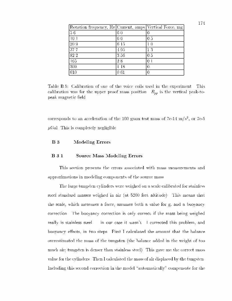
174Rotation frequency, Hz Current, amps Vertical Force, mg5.6 6.0 010.1 6.6 0.520.9 6.15 1.037.7 4.95 1.382.2 3.56 0.5165 2.8 0.1309 1.18 0610 0.61 0

Table B.5: Calibration of one of the voice coils used in the experiment. Thiscalibration was for the upper proof mass position. Bpp is the vertical peak-to-peak magnetic �eld.

corresponds to an acceleration of the 100 gram test mass of 7e-14 m/s2, or 7e-5

�Gal. This is completely negligible.

B.3 Modeling Errors

B.3.1 Source Mass Modeling Errors

This section presents the errors associated with mass measurements and

approximations in modeling components of the source mass.

The large tungsten cylinders were weighed on a scale calibrated for stainless

steel standard masses weighed in air (at 5200 feet altitude). This means that

the scale, which measures a force, assumes both a value for g, and a buoyancy

correction. The buoyancy correction is only correct if the mass being weighed

really is stainless steel | in our case it wasn't. I corrected this problem, and

buoyancy e�ects, in two steps. First I calculated the amount that the balance

overestimated the mass of the tungsten (the balance added in the weight of too

much air; tungsten is denser than stainless steel). This gave me the correct mass

value for the cylinders. Then I calculated the mass of air displaced by the tungsten.

Including this second correction in the model \automatically" compensate for the

175Description Signal, �GalEddy Current Damping < 0�7 �GalDirect Magnetic attraction < 10�6 �GalAC; Magnetic Forces < 10�4 �Gal

Table B.6: Errors due to spurious forces. The e�ects of the source mass arediscussed in Sec. 5.2.2.

gravitational attraction of the displaced air. The total correction to the reading on

the scale was -4.76 grams per cylinder. The uncertainty associated with the mass

of each of the 12 tungsten cylinders and the two aluminum plates (arising from

the scale's accuracy) is �1 gram. The total mass uncertainty (for the cylinders)

was taken as 1g � p14 = 4 g.

In the same way a buoyancy correction was applied to the upper and lower

aluminum plates of the experiment. 1997: the Upper plate was modeled 0.62

grams lighter than its true mass, while the lower plate was made 0.76 grams

lighter. 1998: the lower plate was modeled 1.53 grams lighter and the upper was

made 1.55 grams lighter.

The error in the buoyancy corrections due to barometric pressure changes

(approximately 1% magnitude) is far smaller than the error in weighing, and there-

fore is ignored. In some sense the time-varying barometric pressure correction,

which shifts with pressure, is a variable independent of our signal and is therefore

absorbed in the statistical errors of the experiment.

The mass uncertainty in all other components of the system (about 20 dif-

ferent objects, in which nuts and bolts were weighed as collections) is 0:1 gram.

This leads to a total error estimate of 0:5 g. Grease on the screws collected on the

nuts and thus traveled with the source mass. The weight of a sample of grease of

about the same volume as that on the nuts weighed 5 grams. I couldn't reliably

model this e�ect because the screws were often cleaned. Rather than assume an

176

average perturbation, the whole grease e�ect is accepted as an error.

The measurement of the position of the center-of-mass with respect to the

geometric centers of the tungsten cylinders allowed us to make estimates of errors

from angular and linear density variations within the cylinders. 11 of the 12

tungsten cylinders had an angular density variation producing a torque equivalent

to a 25 gram mass placed on their circumferences. The twelfth mass, however,

(#4) displayed no angular density variation, and was therefore suspect (discussed

in Appendix A). We needed to include an estimate for the error introduced by

these characteristics.

Exactly how to calculate the errors due to these types of sources was not

immediately clear. The position of an unmodeled point mass distribution strongly

in uences the magnitude of the signal error it causes. We decided to assign a

value of 5g as the over all uncertainty in the mass of the source mass, distributed

uniformly about the source mass. We also modeled a 25 gram point mass in the

position that results in the largest signal bias. The possibility of a misplaced

point of mass of 25 grams is of greater probability than an error in the total mass

of this size because a misplaced point mass represents the uncertainty in density

inhomogeneities in the masses. It is interesting that a 25 gram mass placed on the

inner radius near the middle of the source mass results in a bias in the di�erential

signal of 0.01 �Gal, yet if the 25 grams were distributed uniformly around the

source mass, they would have a signal of:

perterbed signal =25g total signal

mass of source mass=

25g

40kg � 12(80�Gal) = 0:005�Gal

(B.3)

This result indicates that even if our source mass were in�nitely dense, our signal

could only be improved by approximately a factor of two (assuming no major

redesign of the FG-5 and conserving the net mass of the source mass)!

177Description Signal, �Gal Signal, ppmMass estimates errors 0.002 25Unmodeled grease andunknown point mass 0.005 60density variations:linear 0.004 50Radial 0.002 25Angular 0.002 25quadratic 0.005 60TOTAL 0.011 110

Table B.7: Uncertainties in proof mass position and orientation

Other approximations in the source mass model were unimportant. The

error from modeling an array of screws as a ring of screws is approximately 2 �10�8�Gal. the thread as part of the screw is approximately 4� 10�9�Gal. Table

B.7 displays the errors associated with modeling of the source mass.

B.3.2 Proof Mass Modeling errors

To scale errors of modeling the proof mass and to discover the degree of

precision required for an adequate model to be constructed, I made three simpli�ed

models of the proof mass. The �rst was a vertical line charge of mass, the same

length as the proof mass. To test the sensitivity of the results to the vertical

\granularity" of the model, the line charge was broken into n point charges, equi-

distant from each other. Figure B.2 displays the di�erences in net accelerations

for the given models falling though a �eld generated by a simpli�ed source mass

model. The data shows that the convergence is better than linear, so with 32

layer model in the vertical direction we expect the error to be less than twice the

maximum di�erence between the acceleration of the 64 layer model and the 32.

This di�erence is 0.0015 �Gal. A vertical granularity corresponding to 64 layers

(1.25 mm/step) was used in the �nal proof mass model.

178

−40 −30 −20 −10 0 10 20 30 40−0.02

−0.015

−0.01

−0.005

0

0.005

0.01

0.015

0.02

Position, cm

Acce

lera

tion

diffe

renc

e, µ

Gal

Figure B.2: Change in vertical acceleration as a function of the vertical granular-ity of model. (|) the di�erence between calculated acceleration for a verticallyoriented line charge of the same length as the actual proof mass, modeled as 64and 32 point masses. (-�-) modeled as 32 vs 16 point masses and (� � �) modeled as16 vs 8 point masses.

I performed a similar test of the horizontal granularity sensitivity by using a

1 cm line-charge radially oriented. Although the proof mass actually extends to a

1.5cm radius, modeling granularity in not an issue at these radii, because the proof

mass portions can be nearly perfectly described as cylinders. The corner cube,

the object most badly approximated by a cylinder, extends to a 0.5 cm radius.

Figure B.3 plots di�erences in accelerations for various granularity models. Using

a radial model granularity of 0.125 cm is adequate for our purposes, introducing

only 0.0012 �Gal error.

In one last test of the sensitivity, in both dimensions at the same time,

179

−40 −30 −20 −10 0 10 20 30 40−5

−4

−3

−2

−1

0

1

2

3

4

5x 10

−3

Position,cm

Acce

lera

tion

diffe

renc

e, µ

Gal

Figure B.3: Change in vertical acceleration as a function of the radial granularityof the model. (|) the di�erence between calculated acceleration for a horizontallyoriented line charge extending from the axis of symmetry to 1 cm o� axis, modeledas 32 and 16 point masses. (� � �) Modeled as 16 vs 8 point masses, (- -) 8 vs 4,and (� � �) 4 vs 2 points.

I modeled an hourglass shaped mass with its axis of symmetry aligned in the

vertical direction. The hourglass was the same height as the actual proof mass,

and of 1 cm maximum radius. The results of this test show that a granularity of

32 slices across the height of 8 cm is satisfactory for the experiment, resulting in

an error that (using the extrapolation to an continuous object) is good to better

than 0.01 �Gal.

This granularity is so coarse that actual modeling errors of reasonable mag-

nitude are not going to a�ect the accuracy of the results strongly. For example,

the proof mass is made up of some objects that are very well modeled as cylinders

| they only di�er from perfect cylinders in that they are imperfectly machined.

When we model these pieces as perfect cylinders, the actual object may vary from

the model by some small fraction of a millimeter: certainly by less than 0.003cm.

Since we only need the granularity to be better than about 0.1 cm, these errors

180

are lost in the glare of large modeling approximations. The fact that many pieces

of the proof mass are very good approximation of cylinders means that adopting

the whole error due to granularity is unreasonable. Because well over half of the

mass is contained in objects which are perfectly described as cylinders to levels

of 0.01 cm, we might halve the error estimates for granularity errors. Since the

errors are so small, however, they are maintained.

The �nal proof mass model was made with a vertical and horizontal gran-

ularity of better than 0.125 cm. This corresponds to an error of 0.0015 �Gal due

to the vertical approximation, and 0.0006 �Gal due to the radial approximation,

for a fully complex object, in a single source mass position.

The model of the proof mass was developed from machine drawings and

measurements of the masses of individual proof mass components. There were

three elements of the model, the corner cube holder, corner cube, and glue that

we weren't able to weigh independently (because they're all glued together). We

weren't able to get their masses by weighing disassembled assemblies because they

aren't very consistent from piece to piece. For this reason we had to estimate2

the mass distribution between the three components. This error introduced by

the uncertainty in this distribution is greater than the combined uncertainty in

all other components of the model.

Only the relative masses of each component of the test mass was important

in our models. Since the components were weighed in air a relative mass error

between materials of di�erent density was introduced. The buoyancy correction

for the optical sphere, for example, is 0.002 grams. This is an order of magnitude

smaller uncertainty in the accuracy of the scale used in the measurements. We

2 We chose to use the greatest mass observed for both the corner cube and the corner cubeholder, and make up the mass di�erence in the binding glue. Our original estimate of the glueweight was based on a similar system, in which a corner cube was glued to a small aluminumcylinder modeled on the corner cube holder. The glue mass used in this system was 0.29 grams,only about 20% lighter than our �nal glue estimate.

181Description Signal, �Gal Signal, ppmradial Model Granularity 0.0012 15 ppmVertical Granularity 0.003 35 ppmRelative Mass Errors(CC, CCholder,Glue) 0.003 35 ppmRelative Position Errors 0.007 80 ppmTotal 0.008 90 ppm

Table B.8: Uncertainties in proof mass position and orientation

made the assumption that all the material of the proof mass was free of voids and

appreciable density variations.

The positions of each element have uncertainties of as much as 0.01 cm. By

modifying the weight and position of individual elements of the the proof mass

model, and testing the output solution, I obtained error estimates of: 0.002 �Gal

in the �nal signal due to a 0.07 cm translation of any of the major proof mass

elements and and error of 0.0009 �Gal due to a 0.1 gram mass error. The proof

mass is built of approximately 10 pieces, so the total error due to incorrect weights

and positions is about 0.007 �Gal.

Table B.8 lists the proof mass modeling errors. The �nal proof mass model

that we used in Appendix A.

B.4 Numerical System

B.4.1 Absolute Accuracy of Quadrature: The Integration Over

the Source Mass

To insure the accuracy of our numerical results we used quadrature algo-

rithms that calculated error estimates for the values they returned. The algorithms

were checked against analytic solutions whenever possible3 . We implemented the

integration algorithms twice, using a straight 4-D integration as a check to the

3 We used analytic solutions for the the case of cylinders with a common axis of symmetry.

182

interpolation scheme discussed in Sec. 2.1. Unfortunately the 4-D integration

was incredibly slow | a full test of the integration over the complete source and

proof mass models could not be performed. Once we were sure that the implemen-

tations were consistent and correct for small systems of masses the interpolation

system (that was used in the �nal calculations) was tested for self-consistency.

The main source of concern was the required density of grid points in the

interpolation �eld to achieve our required accuracy. A standard method of testing

for su�cient density is to double the density until the variation in the �nal values

(integrated over the grid) becomes negligible. Figure B.4 is a plot of the net

acceleration of the proof mass (using a 44 piece model) as a function of the number

of grid points used in the vertical direction. The three plots were all calculated

using the same radial grid density of 30 points/3 cm. The 500 to the 1000 point

accelerations di�er by less than 0.001 /Ugal, as seen in Figure B.5. Results for a

radial grid density of 15 points/3 cm are very similar.

−2.75 −2.7 −2.65 −2.6 −2.55 −2.5 −2.45 −2.4 −2.35 −2.3 −2.2542.7

42.705

42.71

42.715

42.72

42.725

Position, cm

Acce

lerati

on, u

Gal

Figure B.4: Calculated acceleration for a 44 piece proof mass model, using threedi�erent vertical grid densities. The | line represents the acceleration resultingfrom using 250 grid points in the vertical direction (over approximately 90 cm ).The � � � � line results from 500 points, and the -�- line from 1000 points.

183

−40 −30 −20 −10 0 10 20 30 40−2.5

−2

−1.5

−1

−0.5

0

0.5

1

1.5

2

2.5x 10

−3

position, cm

Acce

lerati

on di

fferen

ce, u

Gal

Figure B.5: Di�erences in calculated acceleration for a 44 piece proof mass model,using three di�erent vertical grid densities. The solid line represents the di�erencein accelerations calculated using 1000 grid points and 500 grid points. The dottedplot is the di�erence between the results of a 500 and a 250 point grid. All gridsused had 30 grid points o� axis.

Testing the dependence of calculated acceleration on radial grid density in

the same way insured the appropriate choice of grid size. Figures B.6 and B.7 show

computed results for three di�erent radial grid densities. Based on these results,

the �nal solution was calculated using a vertical grid density of 1000 points/90

cm, and a radial density of 30 points/3 cm. These plots clearly indicate that the

error in the interpolation due to the radial grid density is bound by 0.0005 �Gal .

B.4.2 Assumption of Cylindrical Symmetry

The two-dimensional interpolation grid algorithm assumes that the �eld of

the source mass was cylindrically symmetric. Although the mass is 1-, 2-, 3-, and

6-fold rotationally symmetric4 , it was not cylindrically symmetric. Figure B.8

displays the vertical �eld as a function of angle for each of six cylinders making

up a simpli�ed source mass model. The plots were made for a vertical position

4 To the degree that the masses were perfectly homogeneous. . .

184

−2.75 −2.7 −2.65 −2.6 −2.55 −2.5 −2.45 −2.4

42.716

42.718

42.72

42.722

42.724

42.726

42.728

position, cm

calcu

lated

acce

lerati

on, u

Gal

Figure B.6: Calculated acceleration for a 44 piece proof mass model, using threedi�erent radial grid densities. The | line represents the acceleration resultingfrom using 60 grid points over 3 cm. The � � � � line results from 30 points, and the-�- line from 15 points, over the same range.

−40 −30 −20 −10 0 10 20 30 40−7

−6

−5

−4

−3

−2

−1

0

x 10−4

position, cm

differ

ence

in ca

lculat

ed ac

celer

ation

s, uG

al

Figure B.7: Di�erences in calculated acceleration of a 44 piece proof mass model,using three di�erent grid densities. The solid line represents the di�erence inaccelerations calculated using 30 grid points and 15 grid points over 3 cm. Thedotted plot is the di�erence between the results of a 60 and a 30 point grid. Allgrids used had 500 grid points over 90 cm on the vertical axis.

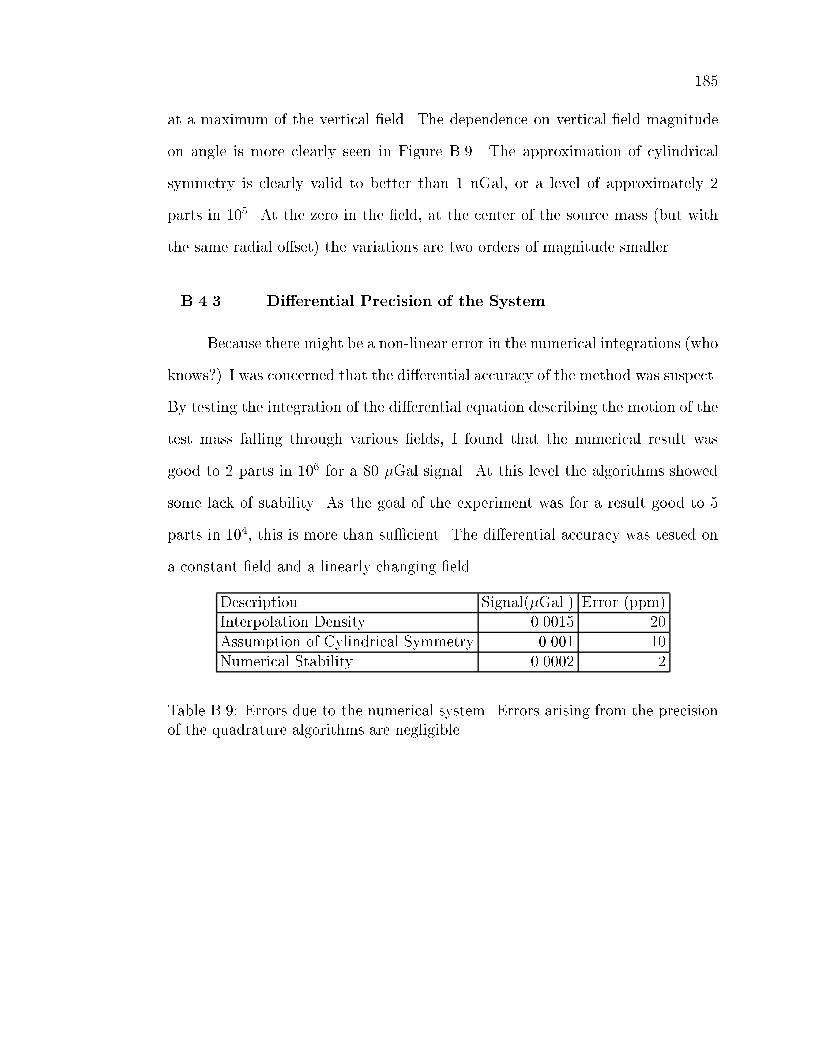
185

at a maximum of the vertical �eld. The dependence on vertical �eld magnitude

on angle is more clearly seen in Figure B.9. The approximation of cylindrical

symmetry is clearly valid to better than 1 nGal, or a level of approximately 2

parts in 105. At the zero in the �eld, at the center of the source mass (but with

the same radial o�set) the variations are two orders of magnitude smaller.

B.4.3 Di�erential Precision of the System

Because there might be a non-linear error in the numerical integrations (who

knows?) I was concerned that the di�erential accuracy of the method was suspect.

By testing the integration of the di�erential equation describing the motion of the

test mass falling through various �elds, I found that the numerical result was

good to 2 parts in 106 for a 80 �Gal signal. At this level the algorithms showed

some lack of stability. As the goal of the experiment was for a result good to 5

parts in 104, this is more than su�cient. The di�erential accuracy was tested on

a constant �eld and a linearly changing �eld.

Description Signal(�Gal ) Error (ppm)Interpolation Density 0.0015 20Assumption of Cylindrical Symmetry 0.001 10Numerical Stability 0.0002 2

Table B.9: Errors due to the numerical system. Errors arising from the precisionof the quadrature algorithms are negligible.

186

0 50 100 150 200 250 300 350 4005

5.5

6

6.5

7

7.5

8

8.5

9

Offset angle, degree

Vertic

al ac

celer

ation

, uGa

l

Figure B.8: Vertical acceleration from a source mass model constructed of sixcylinders. Values are plotted as a function of angle from a line of symmetry, for apoint 2 cm o� axis. Note that that contributions of the individual cylinders (� � � �)are not true cosines( as they would be if the vertical force on the proof mass werea function linear in the distance between the proof mass and the cylinder) becausethey are modulated by the 1

r2factor in the gravitational interaction. The solid

line represents the average acceleration due to each cylinder. As far as this curveapproximates a line, the �eld is cylindrically symmetric.

0 50 100 150 200 250 300 350 400−2

−1.5

−1

−0.5

0

0.5

1

1.5

2x 10

−4

Angular offset, degrees

Vertic

al ac

celer

ation

, uGa

l

Figure B.9: Variation of vertical acceleration as a function of angle when 2 cmo� axis. At a maximum in the �eld, this plot shows that the �eld is cylindricallysymmetric to 0.2 nGal, at a 2 cm radius.