Embed Size (px)
Citation preview

Chapter 2. Literature Review 14
2 Literature Review
2.1 Introduction
The BBC World Service owns and hires MF and HF transmission sites for its
international broadcasting services, where short wave propagation is via earth F2-layer
ionosphere refractions. The transmitters are typically of high power (between 250 and
500kW), broadcasting through high gain curtain antennas. At such sites, the BBC is
obliged to consider the potential risk to its staff and members of the public posed by
radiation from the high power transmitting antennas. The near field region, close to
these antennas is of particular interest from the point of view of both occupational and
public exposure to high RF fields. This is because station boundary fences can be
within one or two wavelengths of the antenna, so the ability to analyses or model the
near field region is important for demonstrating compliance with accepted guidelines.
Guidelines for occupational and public exposure are different. The occupational
guidelines assumed that the individual is of working age and in good health. It is
reasonable to assumed that people who are exposed to radiation through their
occupation will be familiar with the equipment and have received adequate training
[2.1]. The public exposure guidelines assume that the hazard is presented to a person
of any age and in any state of health. It is also unlikely that the public will be aware of
the hazards or the existence of high levels of radiation.
The main objectives of this research are to understand and find a computationally
efficient method for the analysis and prediction of these exposure levels in compliance
with International Commission on Non-Ionising Radiation Protection (ICNIRP) human
exposure guidelines [2.2]. This is necessary to understand the correlation between
energy absorption rates in the body and the risk to health, as well as near-field
distributions of the high power BBC HF broadcasting transmission site.
This chapter provides some background information about the broadcasting antenna
arrays and summarizes basic principles of human exposure safety guidelines. Further
safety criteria required by ICNIRP will be described in following chapter.

Chapter 2. Literature Review 15
A range of research studies are presented. The common objective is to build a
modelling and measurement methodology to assess compliance with ICNIRP EM
exposure guidelines in close proximity to HF transmitting antennas. This chapter gives
a brief review of background information about broadcasting sites and International
guidelines on human RF exposure.
Near field RF conditions are assessed through the use of efficient and accurate
numerical methods, some of which are present in this chapter. They can provide an
insight into how the near field characteristics can be disturbed by the presence of a
person. Two software packages were used to model curtain antennas, Numerical
Computational Code 4 (NEC4) [2.3] and CST Microwave Studio [2.4]. The theory
behind these packages are briefly summarised in Section 2.2. Several software
packages are available on the market and it is beneficial for the user to have some
knowledge of the software engines which they employ and to understand the basic
equations and application methods used by the different numerical codes.
Human phantoms – high resolution numerical models of human beings which
incorporate the electrical properties of the body and its internal organs - are described
in this chapter. The software package SEMCAD and its associated ‘Virtual Family’ of
human phantoms are introduced. Results generated with the Virtual Family [2.5]
associated with the SEMCAD package [2.6] are compared with earlier results
generated using a phantom called ‘Norman’- Normalised Man, a model developed by
the UK HPA (Health Protection Agency – Radiation Protection Division). The
different capabilities and limitations of all these numerical codes are described, and
finally a description of an equivalence principle theory is given. The equivalence
principle was used as part of a hybrid approach to develop a modelling methodology to
solve this EM problem.
This chapter is divided into two sections. First HF broadcasting antenna and
background ICNIRP guidelines, then numerical methods and techniques / Simulation
Software
2.1.1 BBC HF antennas
Until recently, short-wave broadcast transmitters operate in the frequency range 3MHz
to 30MHz. The BBC World Service owned and operated 7 high power transmitting
Chapter 2. Literature Review 16
stations, worldwide, through a contract with Babcock International Group. The BBC
world service uses frequencies between 5 MHz and 23 MHz. The pertinent details are
given in Table 2.1.
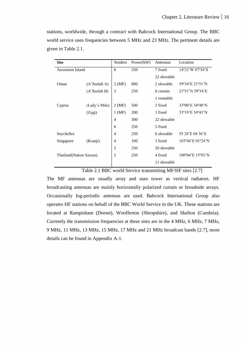
Site Senders Power(kW) Antennas Location
Ascension Island 6 250 7 fixed
22 slewable
14º23’W 07º54’S
Oman (A’Seelah A) 2 (MF) 800 2 slewable 59º34’E 21º51’N
(A’Seelah B) 3 250 6 curtain
1 rotatable
21º51’N 59º34’E
Cyprus (Lady’s Mile) 2 (MF) 500 2 fixed 33º00’E 34º40’N
(Zygi) 1 (MF)
4
6
200
300
250
1 fixed
22 slewable
5 fixed
33º19’E 34º43’N
Seychelles 4 250 6 slewable 55 28’E 04 36’S
Singapore (Kranji) 4
5
100
250
1 fixed
20 slewable
103º44’E 01º24’N
Thailand (Nakon Sawan) 5 250 4 fixed
11 slewable
100º04’E 15º03’N
Table 2.1 BBC world Service transmitting MF/HF sites [2.7]
The MF antennas are usually array and uses tower as vertical radiators. HF
broadcasting antennas are mainly horizontally polarized curtain or broadside arrays.
Occasionally log-periodic antennas are used. Babcock International Group also
operates HF stations on behalf of the BBC World Service in the UK. These stations are
located at Rampisham (Dorset), Woofferton (Shropshire), and Skelton (Cumbria).
Currently the transmission frequencies at these sites are in the 4 MHz, 6 MHz, 7 MHz,
9 MHz, 11 MHz, 13 MHz, 15 MHz, 17 MHz and 21 MHz broadcast bands [2.7], more
details can be found in Appendix A-1.
Chapter 2. Literature Review 17
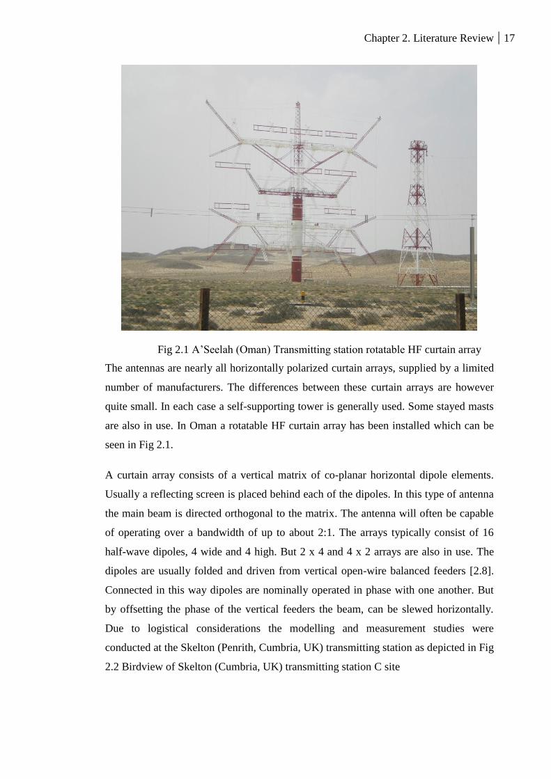
Fig 2.1 A’Seelah (Oman) Transmitting station rotatable HF curtain array
The antennas are nearly all horizontally polarized curtain arrays, supplied by a limited
number of manufacturers. The differences between these curtain arrays are however
quite small. In each case a self-supporting tower is generally used. Some stayed masts
are also in use. In Oman a rotatable HF curtain array has been installed which can be
seen in Fig 2.1.
A curtain array consists of a vertical matrix of co-planar horizontal dipole elements.
Usually a reflecting screen is placed behind each of the dipoles. In this type of antenna
the main beam is directed orthogonal to the matrix. The antenna will often be capable
of operating over a bandwidth of up to about 2:1. The arrays typically consist of 16
half-wave dipoles, 4 wide and 4 high. But 2 x 4 and 4 x 2 arrays are also in use. The
dipoles are usually folded and driven from vertical open-wire balanced feeders [2.8].
Connected in this way dipoles are nominally operated in phase with one another. But
by offsetting the phase of the vertical feeders the beam, can be slewed horizontally.
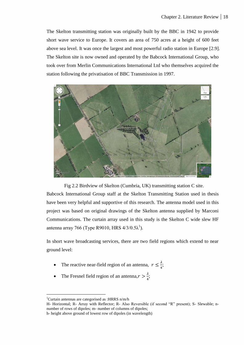
Due to logistical considerations the modelling and measurement studies were
conducted at the Skelton (Penrith, Cumbria, UK) transmitting station as depicted in Fig
2.2 Birdview of Skelton (Cumbria, UK) transmitting station C site
Chapter 2. Literature Review 18
The Skelton transmitting station was originally built by the BBC in 1942 to provide
short wave service to Europe. It covers an area of 750 acres at a height of 600 feet
above sea level. It was once the largest and most powerful radio station in Europe [2.9].
The Skelton site is now owned and operated by the Babcock International Group, who
took over from Merlin Communications International Ltd who themselves acquired the
station following the privatisation of BBC Transmission in 1997.
Fig 2.2 Birdview of Skelton (Cumbria, UK) transmitting station C site.
Babcock International Group staff at the Skelton Transmitting Station used in thesis
have been very helpful and supportive of this research. The antenna model used in this
project was based on original drawings of the Skelton antenna supplied by Marconi
Communications. The curtain array used in this study is the Skelton C wide slew HF
antenna array 766 (Type R9010, HRS 4/3/0.5λ1).
In short wave broadcasting services, there are two field regions which extend to near
ground level:
The reactive near-field region of an antenna,
;
The Fresnel field region of an antenna,
;
1Curtain antennas are categorised as :HRRS n/m/h
H- Horizontal; R- Array with Reflector; R- Also Reversible (if second “R” present); S- Slewable; n-
number of rows of dipoles; m- number of columns of dipoles;
h- height above ground of lowest row of dipoles (in wavelength)

Chapter 2. Literature Review 19
Where r is the distance from the centre of the antenna to the point of investigation.
Fig 2.3 Vatican Radio antenna towers [2.10].
As can be seen in Fig 2.2 most of these high powers broadcasting transmitter stations
are located in unpopulated rural areas. Metal fences and locked gates help to keep the
public a certain distance away from these arrays. There are also some unusual and
uncontrollable cases in short-wave broadcasting. Fig 2.3 Vatican Radio antenna towers
Fig 2.3 Vatican Radio antenna towers [2.10] shows the periphery of the transmitter
station for the Vatican Radio station, which is near Cesano, 12 miles north of Rome. It
is clear from the figure that this station is surrounded by a populous residential area.
Similarly in Singapore the Kranji transmitter station is located on land adjacent to the
main building of a Golf club. To maximize the coverage area MF band (300 kHz-
3MHz) and HF band (3 MHz - 30 MHz) broadcasting transmitters all operate at high
power (Table 2.1), details which can be found in Appendix A-2.
Numerous international scientists have researched the possible health hazards
associated with human exposure to EMF. Recently many of these studies have focused
primarily on the modern telecommunications systems, such as cellular Base Stations.
Studies in this area include those conducted in 2006 by Mobile Telecommunications
and Health Research (MTHR) [2.11], and the German Mobile Telecommunication
Research Programme conducted by The German Commission on Radiological
Protection [2.12]. After a review of these recent studies the ICNIRP concluded that

Chapter 2. Literature Review 20
exposure levels due to cell phone base stations are generally around one-ten-
thousandth of the guideline levels [2.13]. A statement on the topic was published in
2009 by the ICNIRP. It was entitled “Guidelines for limiting exposure to time-varying
electric, magnetic, and electromagnetic fields (up to 300 GHz)” [2.14]. It indicated that
there is a lack of satisfactory individual exposure assessment of low-level, whole-body
exposure in the far-field of radiofrequency (RF) transmitters. A problem for those such
as the BBC World Service and Vatican Radio, are the possible high levels of whole-
body exposure in the near-field of HF high power broadcasting transmitting stations;
there have not been many studies done on this so far. In 2006, the European
Broadcasting Union published the results of a study carried out by the United
Kingdom Health Protection Agency (UK HPA) and commissioned by the BBC World
Service. The purpose of the study was to assess the emission compliance of the BBC
MF [2.15] and HF [2.16] broadcast transmitters against the ICNIRP exposure
guidelines. The HPA applied Finite Difference Time Domain (FDTD) solution of
Maxwell’s curl equations to compute the whole body Specific Absorption Rate (SAR).
In addition, a quasi-static Scalar Potential Finite Difference (SPFD) solution of
Laplace’s equation was used to compute limb SAR as a function of the induced current
[2.17], [2.18]. This was then linked to the whole body incident field strength through
the FDTD algorithm. A human phantom was illuminated with either a vertically or
horizontally polarized plane wave, in various configurations such as: bare-feet
touching the ground, with shoes, isolated; arms at the side, or outstretched [2.15],
[2.16]. It was assumed that in the near-field of an MF antenna the dominant field
component is a uniform and vertically polarized electric field. In this case, the
localised SAR in the leg is the most restrictive quantity [2.2], [2.15].
Prior to these studies by the HPA there was a very limited amount of research which
involved comparing the emission from broadcasting antennas against the ICNIRP
guidelines. Other HPA studies formed the foundation for the guidelines published by
the ICNIRP in 1998. In 1994 Jokela et al measured the emissions from a MF vertical
monopole antenna operating at a frequency of 963 kHz with an input power of 600 kW
[2.19]. This antenna is located in Pori (Finland). Through measurement Jokela et al
discovered that the electric field was 500V/m at 1m above the ground. At 10 m the E-
field strength was found to be 90 V/m. These measurements were made at a distance of
40 m in front of the antenna [2.20]. Jokela et al calculated the current flowing through
Chapter 2. Literature Review 21
the feet of a grounded hemispheroidal model of human. The vertical electric field
induced a current of 140mA at 10m away from the antenna and 30mA at 40 m away
from the antenna. Jokela et al also measured the RF exposure in front of a 500kW HF
curtain array which was operating at 21.55 MHz. The antenna in question is also
located at the Pori broadcasting station. They measured maximum values of electric
field strength and induced current through feet of a grounded human model of 90 V/m,
400mA at a distance of 30 m in front of the antenna. At a distance of 100 m in front of
the antenna they measured 35 V/m, and 75mA. In each case the measurements were
obtained at a height of 1 m above the ground. From 1989 to 1998 Mantiply et al
conducted a series of similar electric field strength measurements [2.21]. Mantiply
studied the exposure level in a community located 10km from six 250 kW HF
transmitters. These transmitters were used to service the Voice of America’s (VOAs)
Delano site in California, United States. These transmitters operate at four different
frequencies, namely: 6.155 MHz, 9.765 MHz, 9.815 MHz, and 11.74 MHz [2.22].
Moreover the electric field strength was measured in front of three other 100kW HF
antennas at distances of 100m, 200m and 300m. These distances were measured 1m
above the ground in the direction of wave propagation. An electrically steerable curtain
antenna (slewable angle ±25°) was also investigated [2.22]. These studies assessed the
EMF level in front of the high power MF and HF antennas. Specifically the E-field
was examined at distances ranging from 10m-10km. The study provides data on the
range of fields values associated with several different types of HF sources. However it
did not provide sufficient information to assess the potential human exposure to the
intense level of HF field.
2.1.2 International Exposure Guidelines and Basic Definitions
Human exposure to electromagnetic radiation is of concern to individuals and
organisations worldwide in relation to the functioning of telecommunications systems.
There are established standards to prevent overexposure to the electromagnetic fields,
present in our environment. Exposure standards for radiofrequency energy have been
developed by various organizations and countries. These standards recommend safe
levels of exposure for both the general public and for workers. The International
Commission on Non-Ionizing Radiation Protection (ICNIRP) is a non-governmental
organization, formally recognized by World Health Organisation (WHO). The
Chapter 2. Literature Review 22
independent scientific experts of the ICNIRP review and evaluate scientific research
literature from all over the world [2.14].
Other countries and regions have taken similar precautions. For example, Canada has
adopted a set of SAR guidelines entitled ‘Limits of Human Exposure to
Radiofrequency Electromagnetic Energy in the Frequency Range from 3 kHz to 300
GHz - Safety Code 6’ [2.23]. This document sets out the requirements and
measurement techniques to be followed when evaluating RF exposure. On the other
hand in the United States, on the other hand, the Federal Communication Commission
(FCC) has adopted safety guidelines for evaluating RF environmental exposure. These
guidelines which have been in place since 1985 [2.24], [2.25]. They were derived from
guidelines produced by the National Council on Radiation Protection and
Measurements (NCRP) and the Institute of Electrical and Electronics Engineers
(IEEE). Many countries in Europe and elsewhere in the world use exposure guidelines
developed by the ICNIRP [2.2], [2.14]. The ICNIRP safety limits are generally similar
to those of the NCRP and IEEE [2.26], [2.27], with a few exceptions. For example, the
ICNIRP recommends different exposure levels in the lower and upper frequency
ranges and for localized exposure due to devices such as hand-held cellular telephones.
The NCRP, IEEE and ICNIRP exposure guidelines identify the same threshold level at
which harmful biological effects may occur. These levels are the basic restrictions.
2.1.3 SAR and Current Density
The Specific Absorption Rate, or SAR, is the rate at which RF energy is absorbed by a
defined amount of mass of a biological body. It is a time derivative of the incremental
energy ( ) absorbed by (i.e. dissipated in) an incremental mass ( ). This
incremental mass is contained within a volume element ( ) of a given density ( )
shown in equation (2.1) [2.28]. The density is measured in units of watts per kilogram
(W/kg). It is a value averaged over pre-defined mass, seen as [2.28]:
(
)
(
) (2.1)
It can also be written as (Equation 2.2):
(2.2)

Chapter 2. Literature Review 23
where: P = Power loss density
E = Electric field strength
J = Current density
σ = Conductivity
ρ = tissue density
To obtain the whole-body averaged SAR the absorption rate in all the cells of the
computational volume must be summed together and then divided by the mass of the
whole body. The averaged SAR, , is given by equation (2.3) [2.29]:
∑
(∑
)
(2.3)
when working with a multilayer cylinder phantom the SAR can be averaged over the
volume of each layer. The equation (2.4) can be written as follows [2.30]:
∑
(∑
)
(2.4)
Where N is the number of the layers in the cylinder phantom is the SAR value
computed in the volume of each cylinder i.
The whole-body averaged SAR is the mean of a distribution which depends on the
frequency, polarization, and the zone of the incident field region. The calculations also
depend on the mass and geometry of the biological body. When the power density of
an incident electromagnetic yield is increased, then the relative increase of the whole-
body SAR will be directly proportional to the increase of any part-body SAR [2.28].
The currents and energy absorption in human body tissue depend on the coupling
mechanisms and the frequency involved. The electric field and current density within
the tissue can be determined by Ohm’s Law: J , where J is the current density in
A/m2, is the electrical conductivity of the medium in S/m, and E is the electric field
strength in V/m. The dosimetric quantities used in by the IEEE and ICNIRP, for
different frequency ranges and waveforms are as follows (Table 2.2):
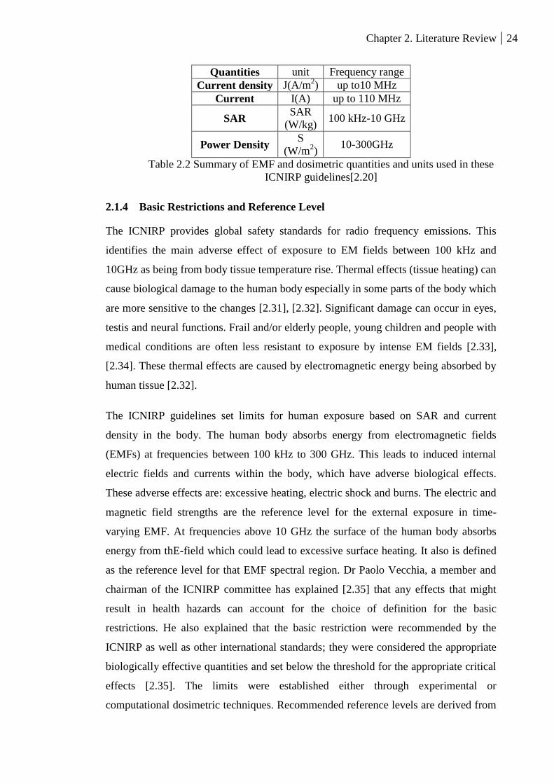
Chapter 2. Literature Review 24
Quantities unit Frequency range
Current density J(A/m2) up to10 MHz
Current I(A) up to 110 MHz
SAR SAR
(W/kg) 100 kHz-10 GHz
Power Density S
(W/m2)
10-300GHz
Table 2.2 Summary of EMF and dosimetric quantities and units used in these
ICNIRP guidelines[2.20]
2.1.4 Basic Restrictions and Reference Level
The ICNIRP provides global safety standards for radio frequency emissions. This
identifies the main adverse effect of exposure to EM fields between 100 kHz and
10GHz as being from body tissue temperature rise. Thermal effects (tissue heating) can
cause biological damage to the human body especially in some parts of the body which
are more sensitive to the changes [2.31], [2.32]. Significant damage can occur in eyes,
testis and neural functions. Frail and/or elderly people, young children and people with
medical conditions are often less resistant to exposure by intense EM fields [2.33],
[2.34]. These thermal effects are caused by electromagnetic energy being absorbed by
human tissue [2.32].
The ICNIRP guidelines set limits for human exposure based on SAR and current
density in the body. The human body absorbs energy from electromagnetic fields
(EMFs) at frequencies between 100 kHz to 300 GHz. This leads to induced internal
electric fields and currents within the body, which have adverse biological effects.
These adverse effects are: excessive heating, electric shock and burns. The electric and
magnetic field strengths are the reference level for the external exposure in time-
varying EMF. At frequencies above 10 GHz the surface of the human body absorbs
energy from thE-field which could lead to excessive surface heating. It also is defined
as the reference level for that EMF spectral region. Dr Paolo Vecchia, a member and
chairman of the ICNIRP committee has explained [2.35] that any effects that might
result in health hazards can account for the choice of definition for the basic
restrictions. He also explained that the basic restriction were recommended by the
ICNIRP as well as other international standards; they were considered the appropriate
biologically effective quantities and set below the threshold for the appropriate critical
effects [2.35]. The limits were established either through experimental or
computational dosimetric techniques. Recommended reference levels are derived from

Chapter 2. Literature Review 25
the basic restrictions. Different limits are set for ‘occupational’ and ‘public’ exposure
arguing that anybody exposed under occupational conditions will be of a certain age
and fitness level while the public might include anybody. As well as the Basic
Restrictions which are based on energy absorption, ICNIRP defines Reference levels
of EM Field Strength. ICNIRP points out that, in general, if the EM Field Strength is
below the Reference Level it can be assumed that the basic restriction will not be
breached [2.2], [2.20].

Chapter 2. Literature Review 26
Basic restrictions Reference levels Reference levels
at 6MHz
*f
Current
density
(mA/m2)
(rms)
**WBSAR
(W/kg)
Localized SAR for
head and trunk
(W/kg)
Localized SAR
for limbs
(W/kg)
*f
E-field
(V/m)
E-field
(V/m)
Occupational
exposure
100kHz-
10MHz f/100 0.4 10 20 1-10MHz 610/f 101
10MH-
10GHz __ 0.4 10 20
10-
400MHz 61 61
General public
exposure
100kHz-
10MHz f/500 0.08 2 4 1-10MHz 87/f1/2 35
10MH-
10GHz __ 0.08 2 4
10-
400MHz 28 28
Table 2.3 ICNIRP basic restrictions and reference levels for HF frequency band [2.2] *f as indicated in the frequency range
**WBSAR: Whole-body average SAR
Chapter 2. Literature Review 27
The ICNRP requires that the localized SAR is averaged over any 10g of contiguous
tissues. ANSI/IEEE whole-body SAR is averaged over the entire body, and partial-
body SAR is averaged over any 1g of tissue defined as a tissue volume in the shape of
a cube. SAR for hands, wrists, feet and ankles is averaged over any 10g of tissue
defined as a tissue volume in the shape of a cube. Different exposure limits are applied
to some devices when only part of the human body is exposed to the radiation. Such
limits apply to mobile phones and base stations. Numerous research studies have been
carried out to assess human exposure to these low power devices. T.G. Cooper et al
[2.36] of the United Kingdom National Radiation Protection Board (NRPB) measured
the radio wave power density in the vicinity of 20 U.K. Microcell and Picocell mobile
base stations. He summarized his finding in a report on general public exposure. In
1994 P.J. Dimbylow and S. Mann constructed a human head model from MRI scan
slices [2.37]. They then applied the Finite Differential Time Domain (FDTD)
technique to calculate SAR in the head model expose in an early mobile handset model.
In 2009 Martínez-Búrdalo, M et al [2.38] also used FDTD to assess the human
exposure to EMF from wifi and Bluetooth devices. They used a XFDTD platform
generated by REMCOM [2.39] and another magnetic resonance imaging (MRI) image
based upon a human head model produced by the Hershey Medical Centre in
Pennsylvania, United States. The next section of this thesis provides further details on
the limits specified in the exposure guidelines.
2.1.5 Voxel Phantoms
A phantom is used to model the human body and evaluate the risks associated with
human exposure to RF fields. The phantom could be either a physical or numerical
model of the whole body or of specific organs. Various types, methods, materials types
of phantom have been developed to model the electrical properties of a human.
Through theoretical studies and analysis, earlier researchers have developed simple
human models. In 1979 Habib Massoudi developed multi-layered cylindrical models
of men. These models were used to study the absorption of energy from plane waves at
frequencies between 0.4 GHz and 8 GHz [2.30]. In 1980 I Chatterjee used multi-
layered slab models in conjunction with the plane wave spectrum (PWS) technique to
calculate the energy absorption at 2.45 GHz [2.40]. Around the same time, another
relatively coarse inhomogeneous human model was used to calculate SAR [2.41],
Chapter 2. Literature Review 28
[2.42]. This model consisted of various blocks having dielectric properties that
matched those of several human organs. The technique involved the use of the Method
of Moments (MoM) Since the 1990s advanced medical diagnostic techniques, such as
magnetic resonance imaging (MRI), computed tomography (CT) etc. have been
employed to develop realistic high resolution voxel models. Human coupling with the
induced field are the main cause for the human biology reactions. The factors of effects
have been quantified as SAR, induced electric field, and current density. These
quantities depend on the frequency of the applied RF field and tissue type (i.e.
dielectric properties). In order to study and understand the correlation between these
physical quantities and the induced biological response, the simulations calculate a
region of specific tissue mass for averaging. In order to obtain more accurate results a
human phantom incorporating greater spatial detail is required. Moreover, the age,
gender and posture of exposed limbs were studied in order to gain a better
understanding of their relevance in the risk assessment [2.43], [2.44], [2.45]. The
exposure problem associated with modern communication systems has become more
complicated as technologies have developed in the past 10 years. High resolution
anatomical human phantoms play an important role in evaluating the risk associated
with human exposure to RF fields. These models are used in the calculation of SAR,
induced electric field and current density. Chapter 3 provides a more detailed
description of the human phantoms have been used in this research.
2.2 Numerical Methods and Techniques
The NEC4 modelling package is based on the Method of Moments, which is an
efficient and accurate technique; it is more suited to model wires and linear dielectrics.
SEMCAD and CST microwave studio are commercial simulation packages based on
finite element codes. These codes are suited to modelling complex inhomogeneous
geometries such as the human body. However, compared with NEC4, these packages
are very expensive and inefficient for modelling large electrical radiation problems. In
fact none of the commercial codes currently available are well suited to this
electromagnetic problem studied in this thesis. The array and its surrounding structure
and environments are electrical large and complex. SEMCAD has advantage of SAR
calculation but less efficient on the field distributions investigation. CST did not have
human phantom until earlier 2011. It is impractical to measure the SAR, induced
Chapter 2. Literature Review 29
electric field, or current density within a human body directly. For this reason the
evaluation of SAR within a human body is generally based on results obtained through
numerical modelling and simulation. It is helpful to correlate the results obtained
through different approaches in order to validate the simulated and derived results. The
following subsections aim to give a basic introduction to the numerical techniques
which form the foundation of several commercial simulation packages, such as CST
Microwave Studio, [2.4], SEMCAD [2.6], and NEC4 [2.46].
2.2.1 Method of Moments
The method of moments was developed by Roger F. Harrington [2.47]. The Laurence
Livermore National Labs devised efficient ways to use the method of moments to
solve problems that arise during the design of wire and wire array antennas. NEC4 is a
numerical code written in FORTRAN with a single interface [2.46], and has been
widely used to model wire based antennas. New developments have extended the
applications of MoM to enable 3D EM modelling of wires and flat PEC scatters,
through the use of a triangular mesh [2.48]. The MoM applies orthogonal expansions
to translate the integral equations into a set of simultaneous linear equations. Basis
functions and coefficients matrix methods are used to expand, invoke and solve the
current distributions [2.49]. The procedure to find a solution begins by defining the
unknown current distribution in terms of an orthogonal set of basic functions.
Sub-domain basis functions are used to subdivide a wire into small segments and
model the current distribution on each [2.47]. The shape of the sub-domain basis
functions can vary depending on geometry of the objects to be modelled. Typically
rectangle, triangle, or sinusoidal basis functions are used in MoM. The amplitude of
these constructs is represented using expansion function coefficients, while a Fourier
series is used to represent the current distributions along the entire wire[2.3]. Finally
the antenna’s radiation characteristics and feed point impedance are derived from the
calculated current distribution (equation 2.5 and 2.6).
∑
(2.5)
where
Chapter 2. Literature Review 30
∫
⁄
[
]
(2.6)
= expansion coefficient associated with the current
= basis function
The boundaries conditions are satisfied by solving the integral equation obtained
through the use of Green’s functions. The electric field integral equation 2.7 (EFIE)
and Magnetic field integral (equation 2.8) (MFIE) are the primary formulations of
MoM which can be derived from Maxwell Equations [2.3].
EFIE (2.7)
MFIE (2.8)
Where E = the electric field Strength integral equation, H = the magnetic field strength
integral equation and J equals the induced current.
After introducing the integral equation into equations (2.5) and (2.6) we obtain two
new equations 2.9 and 2.10:
∑
(2.9)
∫
⁄
(2.10)
Where is the testing function has a non-zero value for only a small segment of
wire located at z=zm. This operation yields a set of integral equations (Equation 2.11-
2.14) and can be written in matrix form as
[ ][ ] [ ] (2.11)
Where
∫
⁄
(2.12)
(2.13)

Chapter 2. Literature Review 31
∫
⁄
(2.14)
The linear equations will yield the value of
[ ] [ ] [ ] (2.15)
The unknown induced current is now obtained by solving the system of equation
(2.15), given above [2.3]. Other parameters such as the scattered electric and magnetic
fields can be calculated directly from the induced currents. However the Numerical
Electromagnetics code (NEC), is a MoM based code that is mainly used to solve
problems involving sets of linear elements or PEC plate scatters such as wires and
patches. It is very efficient when applied to volume dielectric objects such as
homogeneous multi-layer biological human models. Unfortunately it cannot handle
inhomogeneous phantoms. However the NEC method supports the rapid analysis of
wire conductors. This makes it suitable for modelling HF curtain arrays efficiently.
Since SAR is the main concern in human exposure research, chapter 3 will show how
this SAR can be analysed using the FDTD and FEM methods.
2.2.2 Finite Difference Time Domain Method
In 1966Yee implemented interleaved components in a Cartesian grid. In 1975 Taflove
introduced a stability criteria along with a 3D grid [2.50]. In 1980 Taflove coined the
term Finite Difference Time Domain (FDTD) method [2.51]. In 1981 Mur developed
absorbing boundary conditions [2.52]. By the 1990’s sufficient computer processing
power was available to handle complex problems. The FDTD method is intuitive to
use, easy to implement, robust and flexible. Consequently it is used in a wide variety
of applications and can also handle complex and heterogeneous objects. Effectively the
FDTD method represents a direct solution of Maxwell’s time dependent curl equations
(2.15 and 2.16), which can be written as follows[2.53]:
(2.16)
(2.17)
where H is the magnetic field intensity (A/m),

Chapter 2. Literature Review 32
E is the electric field intensity (V/m),
B is the magnetic flux density (W/m²),
D is the electric flux density (D/m²),
is the magnetic current (V/m²),
is the electric current (A/m²).
The FDTD algorithm is based on a description of the time stepping procedure as
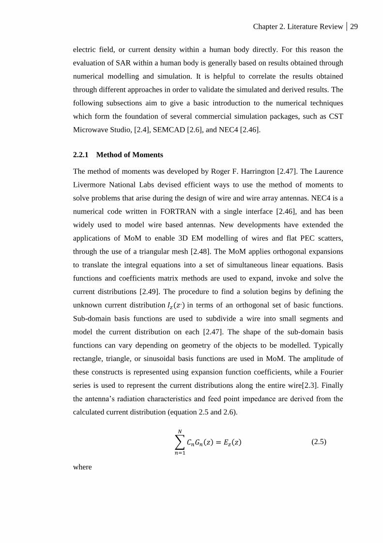
described in equations 2.15 and 2.16. Fig. 2.4 depicts the position of two interleaved
grids of discrete points. One point contains evaluated electric field (yellow)
components in the primary Yee cell while magnetic field (green) components are
evaluated in a secondary Yee cell. Both are allocated within the staggered Cartesian
grid. Each of the E-field vector nodes is surrounded by field components on the basis
of a finite central difference approximation and corresponding to the Faraday and
Ampere’s Law. The i, j, k axis of the FDTD grid represent a 3D volume element.
These axes are aligned with the x, y, z axes of the Cartesian grid.
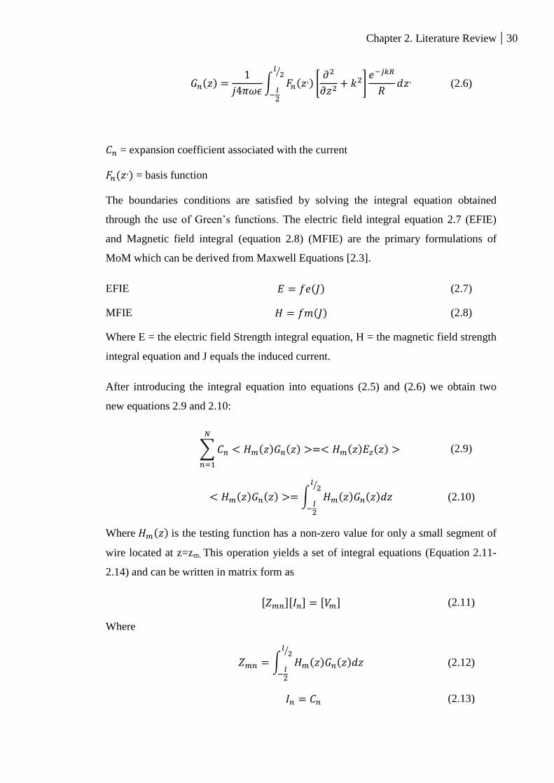
The discretization in time, required to implement the FDTD method, is performed in a
leap-frog manner by application of a temporally shifted update of the E and H field
components [2.53]. This is illustrated in Fig. 2.5.
Thereby the E-field components are calculated at a time increment t = (n+l) , (l = 0, 1,
2 ...) [2.53]. The computation of the H field components in FDTD method is
performed at t = (n + l + 1/2) , (l = 0, 1, 2 ...), i.e. shifted by half a time step. The
time step is defined by equation 2.16.
Chapter 2. Literature Review 33
Fig 2.4 3D Basic Element of the FDTD Yee cell [2.54].
Fig 2.5 Leap-frog scheme in FDTD [2.53].
The time-stepping will stop when a steady state solution or the desired response is
obtained[2.53]. At each time step, the equations used to update the E-field components
are fully explicit and there is no need to solve a system of linear equations. The
technique requires the computer storage and running time proportional to the electrical
size of the volume being modelled as well as he mesh grid cell size or the grid
resolution.
The mesh grid cell size can be set to any fraction of a wavelength. Increasing or
decreasing the mesh resolution, but the time step is inversely proportional to the
maximum grid cell size. The mesh grid cell size needs to satisfy the Courant-
Friedrichs-Levy (CFL) stability condition (Equation 2.18) [2.55].

Chapter 2. Literature Review 34
√
√( )
( )
( )
(2.18)
where c = speed of light in a vacuum, x, x, and z = the cell grid size in the X, Y
and Z directions, respectively; ε = permittivity (F/m), μ is the permeability (H/m)
When the cell grid is uniform in all directions, the equation can be reduced to equation
2.19 [2.55].
√ (2.19)
Therefore, a high resolution mesh requires a smaller time step. Since the E-fields need
to be evolved in the computational domain evolve over time, if a small time step is
employed a larger number of iterations will be required to achieve convergence [2.55].
This is one of the main concerns for this study. In order to calculate the maximum
value of energy absorbed in the human tissue the calculation is performed over all the
cells. Subsequently the result is averaged over either 1g or 10g of tissue within a given
time [2.53]. Different countries and regions follow different standards when
considering the SAR. For example in America the FCC emission standard for cell
phones is 1.6 W/Kg averaged over 1g of tissue, whereas the IEEE and ICNIRP
standards, which apply in Europe, specify 2.0 W/Kg averaged over 10g of tissue. Other
researchers have pointed out a SAR of 2 W/Kg averaged over 10g is approximately
equivalent to an SAR of 4-6 W/Kg average over 1g [2.20]. Chapter 3 describes an
analytical method which was developed to simulate the human phantom exposure to
RF fields. The method involves the use of SEMCAD.
2.2.3 Finite Integration Technique
CST Microwave Studio [2.4] is a general-purpose electromagnetic simulator which
uses the Finite Integration Technique (FIT) to solve problems in electrostatics and
magneto statics. The solver can also be used to handle low frequency and high
frequency problems. The FIT was first proposed by Weiland in 1976 [2.56]. The
technique yields excellent linear scaling of computational resources with structure size.
FIT in the time domain is very similar to the Finite Difference Time domain Technique
(FDTD) introduced by Yee in 1966 [2.54]. They are often are called ‘sister’ 3D
Chapter 2. Literature Review 35
computational techniques. FDTD uses approximations to the spatial and the temporal
(t) derivatives within Maxwell’s equations (i.e. equations 2.14 and 2.15). FIT, on the
other hand, FIT employs the integral form of Maxwell’s equations [2.55] (i.e.
equations 2.20to 2.23).
∮
∫
(2.20)
∮
∫(
)
(2.21)
∮
∫
(2.22)
∮
(2.23)
E is the electric field intensity (V/m),
B is the magnetic flux density (W/m²),
D is the electric flux density (D/m²),
is the current density(A/m²),
ρ is the volume charge density (q/ m²),
A is the element area (m²),
V is the element volume (m3).
Like FDTD, FIT is based on creating a suitable mesh system. This involves splitting
the computational domain up into many small grid cells, as shown in Fig 2.3

Chapter 2. Literature Review 36
Fig 2.6 3D CST microwave studio mesh grids [2.4]
In the case of Cartesian grids, the FIT formulation can be rewritten in the time domain
to yield the standard Finite Difference Time Domain (FDTD) method. Upon applying
the discretized divergent forms of Faraday’s law and Ampere’s law we obtain a
complete set of Maxwell Grid Equations. Finally the material relations (i.e. dielectric
properties) are employed to enable electromagnetic field problems to be solved on the
discrete grid space. Classical FDTD methods involve making a staircase
approximation to complex geometrical boundaries. However, the FIT can implement
the perfect boundary approximation (PBA) along with the thin sheet meshing
technique (TST). By making use of these techniques it is possible to produce an
accurate model of thin curved and sheets of perfect electrical conductors in additional
to staircase approximations [2.55]. The Courant-Friedrichs-Levy (CFL) (equation 2.14)
criterion still has to be fulfilled in every single mesh cell to insure that the explicit time
integration schemes are conditionally stable [2.55].
2.2.4 Boundary conditions
The perfectly matched layer (PML) boundary conditions used in chapter 3 [2.57] were
used. This involves creating a non-physical absorbing medium, adjacent to the external
grid boundary, which causes waves of arbitrary frequency and angle of propagation to
decay rapidly whilst maintaining the correct wave velocity and impedance within the
media from which they originated..
e: electric voltage h: magnetic voltage
b: magnetic flux d: electric flux

Chapter 2. Literature Review 37
2.2.5 Numerical Simulation Software and Techniques
There are several types of commercially available EMF simulation software, although
they are somewhat expensive. Table 2.6 lists some well tested EMF simulation
software packages.
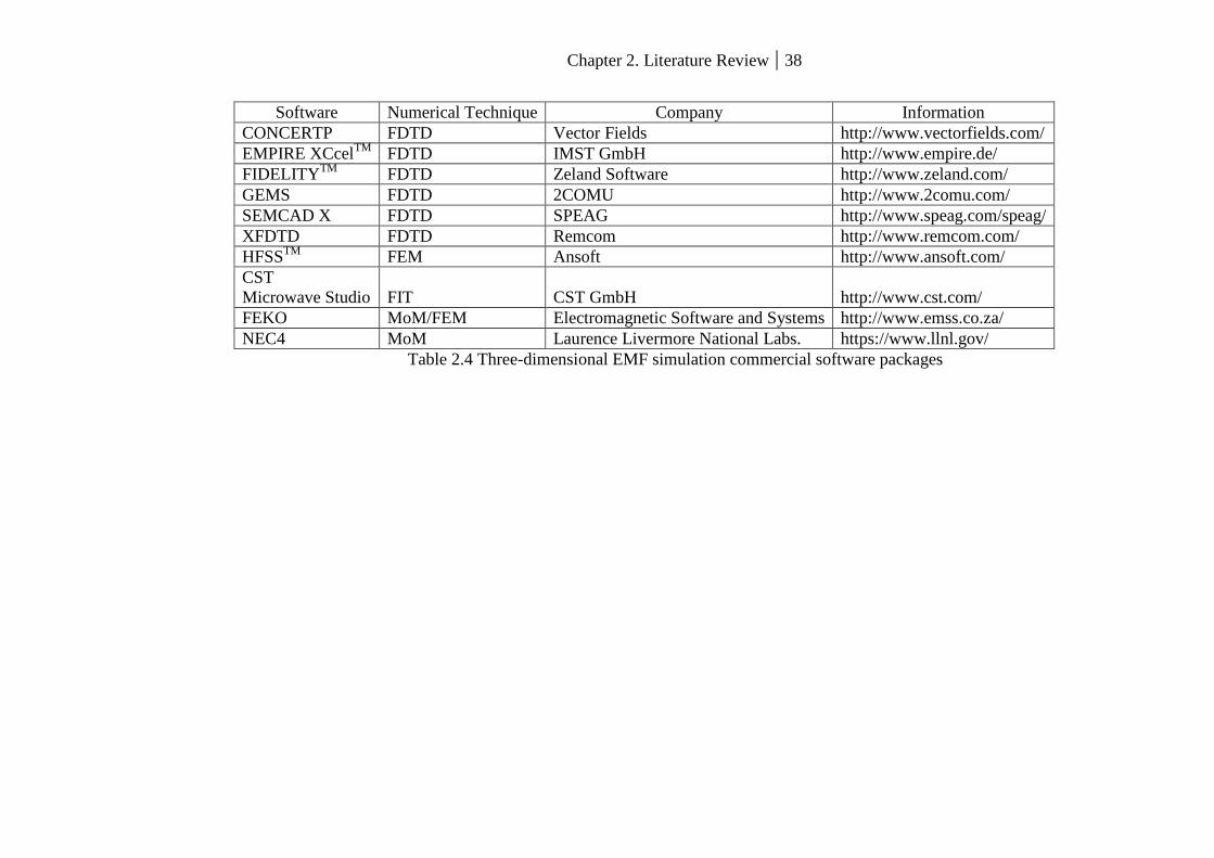
Chapter 2. Literature Review 38
Software Numerical Technique Company Information
CONCERTP FDTD Vector Fields http://www.vectorfields.com/
EMPIRE XCcelTM
FDTD IMST GmbH http://www.empire.de/
FIDELITYTM
FDTD Zeland Software http://www.zeland.com/
GEMS FDTD 2COMU http://www.2comu.com/
SEMCAD X FDTD SPEAG http://www.speag.com/speag/
XFDTD FDTD Remcom http://www.remcom.com/
HFSSTM
FEM Ansoft http://www.ansoft.com/
CST
Microwave Studio FIT CST GmbH http://www.cst.com/
FEKO MoM/FEM Electromagnetic Software and Systems http://www.emss.co.za/
NEC4 MoM Laurence Livermore National Labs. https://www.llnl.gov/
Table 2.4 Three-dimensional EMF simulation commercial software packages
Chapter 2. Literature Review 39
The numerical methods used in this thesis have briefed their application and
limitations in this section. Considering the EM problem encountered in this research,
there are few issues need to address here, when chose a suitable modelling and
simulation tools are important for this research. From Table 2.6 it is clear that CST
microwave Studio is based on the FEM method, SEMCAD uses the FDTD method,
while the NEC4 code is based on MoM. For this reason these software packages are
suitable for solving different problems:
NEC, which uses Moment Method, is most suitable for generating models of
wire antennas while the CST Microwave Studio and SEMCAD uses the Finite
handle volume problem space with anatomy human phantom implementation.
Problems involving open boundaries can be accounted for in NEC using MoM,
while absorbing boundary conditions have to be introduced in both CST
Microwave Studio and SEMCAD.
The two sets of inhomogeneous human phantoms were devised and compared
for the purpose of this thesis. The first phantom was produced in CST
Microwave Studio whilst the second was generated in SEMCAD. The MoM is
efficient both in terms of cost and computational time, while the packages
based on Finite Integration and the Finite Difference Time Domain techniques,
namely CST Microwave Studio and SEMCAD, require extra hardware to
accelerate the computation of problems involving human bodies in order to
avoid excessive processing times.
CST microwave studio and SEMCAD boundary conditions could not be
redefine the dielectric properties, NEC have various realist ground
A novel MoM-FDTD hybrid approach could provide a possible solution to
solve the problems addressed previously.
These summery will hopefully provide a guide to the numerical problem have
encountered and solutions was considered and applied.
2.2.6 Equivalence Principles
The Equivalence Principles Method is a three dimensional representation of the surface
equivalence theorem for a hybrid numerical method was studied in chapter 5. This
theorem replaces electromagnetic sources by equivalent ones; whereby the E-fields
Chapter 2. Literature Review 40
outside an imaginary closed surface are obtained by placing suitable electric and
magnetic current densities over an imaginary closed surface that satisfies the desired
boundary conditions. These current densities are selected so that the resultant fields are
zero within the closed surface. The E-fields should be equal to the radiation produced
by the actual electromagnetic sources outside the closed surface.
The technique can be used to obtain the E-fields radiated outside a closed surface by
referring to sources enclosed within it. Consider an electromagnetic field (E1, H1) in
free space, generated by physical electric and magnetic current sources J1 and M1. Now
assume that J1 and M1 are removed, and that a new field (E, H) can be seen to exist
inside our imaginary surface. And act as a closed source S, the electric and magnetic
currents flowing outside the closed surface S must still satisfy the electromagnetic field
boundary conditions on the tangential E and H fields theoretically using Green’s
theorem as defined by [2.58]:
(2.24)
(2.25)
Where n
is the unit outward normal vector to the closed source S.
2.3 Conclusion
This thesis is concerned with research into radiofrequency exposure and international
human health and safety guidelines. These basic restrictions and reference levels aim
to prevent adverse health effects due to EMF exposure. Background theory and
relevant research is documented here to enable the reader to develop a basic
understanding of what is required for the following chapters of this thesis. Specifically
this chapter provides a brief introduction to the commercial simulation software
packages and other numerical domestric methods and techniques used in this research.
The overall aim of the research presented in this thesis is to use appropriated numerical
domestric methods to assess the risk of human exposure to high power HF
broadcasting transmitter sites.

Chapter 2. Literature Review 41
References
[2.1] IEEE International Committee, “IEEE C95. 1-1992: IEEE Standard for Safety
Levels with Respect to Human Exposure to Radio Frequency Electromagnetic
Fields, 3 kHz to 300 GHz, The,” Inc., New York, NY, vol. 2005, no. April, 1992.
[2.2] International Commission on Non-Ionizing Radiation Protection, “Guidelines
for limiting exposure to time-varying electric, magnetic, and electromagnetic
fields (up to 300 GHz),” Heal. Phys., vol. 74, no. 4, p. 494, 1998.
[2.3] G. J. Burke, “Numerical Electromagnetics Code NEC-4 Mothod of Moments
Part II: Program Description-Theory,” 1992.
[2.4] “CST MICROWAVE STUDIO®.” CST STUDIO SUITE®
http://www.cst.com/.
[2.5] “Virtual Family Phantom®.” The IT’IS Foundation
http://www.itis.ethz.ch/news-events/news/virtual-population/.
[2.6] SPEAG, “SEMCAD X®.” Schmid &Partner Engineering AG
http://www.speag.com/.
[2.7] “Basic standard on Short Wave broadcasting ( 3-30 MHz ),” TC106, BSI
Technical Cttee GEL/106,, 2007.
[2.8] C. Gandy, “R & D White Paper WHP132,” 2006.
[2.9] “Skelton memories,” The British Broadcasting Corporation. [Online]. Available:
http://www.bbceng.info/Operations/transmitter_ops/Reminiscences/skelton/sk1.
htm#8.
[2.10] “Vantican Radio.” [Online]. Available:
http://emfinterface.wordpress.com/2010/07/15/vatican-radio-waves-blamed-for-
high-cancer-risk/.
[2.11] T. G. Cooper, S. M. Mann, M. Khalid, and R. P. Blackwell, “Public exposure to
radio waves near GSM microcell and picocell base stations.,” J. Radiol. Prot.
Off. J. Soc. Radiol. Prot., vol. 26, no. 2, pp. 199–211, 2006.
[2.12] German Commission on Radiological Protection, “German Mobile
Telecommunication Research Programme ( DMF ) Deutsches Mobilfunk-
Forschungsprogramm Stellungnahme der Strahlenschutzkommission,” 2008.
[2.13] International Commission on Non-Ionizing Radiation Protection, “Exposure to
high frequency electromagnetic fields, biological effects and health
consequences (100 kHz-300 GHz),” ICNIRP 16/ …2, pp. 257–258, 2009.
[2.14] International Commission on Non-Ionizing Radiation Protection, “ICNIRP
statement on the ‘Guidelines for limiting exposure to time-varying electric,
Chapter 2. Literature Review 42
magnetic, and electromagnetic fields (up to 300 GHz)’.,” Health Phys., vol. 97,
no. 3, pp. 257–8, 2009.
[2.15] P. Dimbylow, “Assessing the compliance of emissions from MF broadcast
transmitters - including exposure guidelines,” 2006.
[2.16] P. Dimbylow, “Assessing the compliance of emissions from HF broadcast
transmitters - with exposure guidelines,” 2006.
[2.17] P. J. Dimbylow, “The calculation of induced currents and absorbed power in a
realistic, heterogeneous model of the lower leg for applied electric fields from
60 Hz to 30 MHz.,” Phys. Med. Biol., vol. 33, no. 12, pp. 1453–68, Dec. 1988.
[2.18] P. J. Dimbylow, “Current densities in a 2 mm resolution anatomically realistic
model of the body induced by low frequency electric fields.,” Phys. Med. Biol.,
vol. 45, no. 4, pp. 1013–22, Apr. 2000.
[2.19] K. Jokela, L. Puranen, and O. P. Gandhi, “Radio frequency currents induced in
the human body for medium-frequency/high-frequency broadcast antennas.,”
Health Phys., vol. 66, no. 3, pp. 237–44, Mar. 1994.
[2.20] International Commission on Non-Ionizing Radiation Protection, “Exposure to
high frequency electromagnetic fields, biological effects and health
consequences (100 kHz-300 GHz),” ICNIRP 16/ …, 2009.
[2.21] E. D. Mantiply, K. R. Pohl, S. W. Poppell, and J. A. Murphy, “Summary of
measured radiofrequency electric and magnetic fields (10 kHz to 30 GHz) in the
general and work environment.,” Bioelectromagnetics, vol. 18, no. 8, pp. 563–
577, 1997.
[2.22] E. D. Mantiply, K. R. Pohl, S. W. Poppell, and J. a Murphy, “Summary of
measured radiofrequency electric and magnetic fields (10 kHz to 30 GHz) in the
general and work environment.,” Bioelectromagnetics, vol. 18, no. 8, pp. 563–
77, Jan. 1997.
[2.23] E. H. ProtectionBranch, “Limits of Human Exposure to Radiofrequency
Electromagnetic Fields in the Frequency Range from 3 kHz to 300 GHz Limits
of Human Exposure to Radiofrequency Electromagnetic Fields in the Frequency
Range from 3 kHz to 300 GHz,” 1999.
[2.24] “FCC 02-48: FCC Revision of part 15 of the Commission’s rules regarding
ultra-wideband transmission systems. ET-Docket 98-153,” 2002.
[2.25] R. F. J. Cleveland, Compliance with FCC exposure guidelines for
radiofrequency electromagnetic fields, vol. 3. IEEE, 2004, pp. 1030–1035.
[2.26] National Council on Radiation Protection and Measurements, “ADVISING
THE PUBLIC National Council on Radiation Protection and Measurements A
Document for Public Comment,” Bethesda, Maryland, 1994.

Chapter 2. Literature Review 43
[2.27] IEEE International Committee on Electromagnetic Safety, “IEEE Standard for
Safety Levels with Respect to Human Exposure to Radio Frequency
Electromagnetic Fields , 3 kHz to 300 GHz,” Inc., New York, NY, vol. 2005, no.
April, p. 250, 1992.
[2.28] A. ANSI, “IEEE C95. 1-1992: IEEE Standard for Safety Levels with Respect to
Human Exposure to Radio Frequency Electromagnetic Fields, 3 kHz to 300
GHz, The,” Inc., New York, NY, vol. 2005, no. April, 1992.
[2.29] P. J. Dimbylow, “FDTD calculations of the whole-body averaged SAR in an
anatomically realistic voxel model of the human body from 1 MHz to 1 GHz.,”
Phys. Med. Biol., vol. 42, no. 3, pp. 479–90, Mar. 1997.
[2.30] H. Massoudi and C. Durney, “Electromagnetic absorption in multilayered
cylindrical models of man,” … IEEE Trans., vol. M, no. 10, 1979.
[2.31] “FDTD electromagnetic and thermal analysis of interstitial hyperthermic
applicators,” IEEE Trans. Biomed. Eng., vol. 42, no. 10, p. 973, 1995.
[2.32] D. K. Kido, T. W. Morris, J. L. Erickson, D. B. Plewes, and J. H. Simon,
“Physiologic changes during high field strength MR imaging.,” AJR. Am. J.
Roentgenol., vol. 148, no. 6, pp. 1215–8, Jun. 1987.
[2.33] J. R. Jauchem, K. L. Ryan, and M. R. Frei, “Cardiovascular and thermal effects
of microwave irradiation at 1 and/or 10 GHz in anesthetized rats.,”
Bioelectromagnetics, vol. 21, no. 3, pp. 159–166, 2000.
[2.34] E. R. Adair and D. R. Black, “Thermoregulatory responses to RF energy
absorption.,” Bioelectromagnetics, vol. Suppl 6, no. September 2002, pp. S17–
38, Jan. 2003.
[2.35] International Commission on Non-Ionizing Radiation Protection, “Exposure of
humans to electromagnetic fields. Standards and regulations.,” Ann. Ist. Super.
Sanita, vol. 43, no. 3, pp. 260–7, Jan. 2007.
[2.36] T. G. Cooper, S. M. Mann, M. Khalid, and R. P. Blackwell, “Public exposure to
radio waves near GSM microcell and picocell base stations.,” J. Radiol. Prot.,
vol. 26, no. 2, pp. 199–211, Jun. 2006.
[2.37] P. J. Dimbylow and S. M. Mann, “SAR calculations in an anatomically realistic
model of the head for mobile communication transceivers at 900 MHz and 1.8
GHz.,” Phys. Med. Biol., vol. 39, no. 10, pp. 1537–53, Oct. 1994.
[2.38] M. Martínez-Búrdalo, a Martín, a Sanchis, and R. Villar, “FDTD assessment of
human exposure to electromagnetic fields from WiFi and bluetooth devices in
some operating situations.,” Bioelectromagnetics, vol. 30, no. 2, pp. 142–51,
Feb. 2009.
[2.39] “XFdtd®.” Remcom http://www.remcom.com/xf7.

Chapter 2. Literature Review 44
[2.40] I. Chatterjee, M. J. Hagmann, and O. P. Gandhi, “Electromagnetic absorption in
a multilayered slab model of tissue under near-field exposure conditions.,”
Bioelectromagnetics, vol. 1, no. 4, pp. 379–388, 1980.
[2.41] I. Chatterjee, “Electromagnetic-energy deposition in an inhomogeneous block
model of man for near-field irradiation conditions,” Microw. Theory …, pp.
337–340, 1980.
[2.42] M. Hagmann, “Numerical calculation of electromagnetic energy deposition for a
realistic model of man,” Microw. Theory …, pp. 804–809, 1979.
[2.43] P. Dimbylow and R. Findlay, “The effects of body posture, anatomy, age and
pregnancy on the calculation of induced current densities at 50 Hz.,” Radiat.
Prot. Dosimetry, vol. 139, no. 4, pp. 532–8, Jun. 2010.
[2.44] Y. Kawamura and T. Hikage, “Whole-body averaged SAR measurements of
postured phantoms exposed to E-/H-polarized plane-wave using cylindrical field
scanning,” Antennas …, no. 3, pp. 676–679, 2012.
[2.45] “Effects of posture on FDTD calculations of specific absorption rate in a voxel
model of the human body,” Phys. Med. Biol., vol. 50, no. 16, p. 3825, 2005.
[2.46] “Numerical Electromagnetics Code NEC-4.” University of California,
Livermore, Ca 94551, Technical Information Dept., Lawrence Livermore
National Laboratory.
[2.47] R. Harrington, “Matrix methods for field problems,” Proc. IEEE, vol. 55, no. 2,
p. 136, 1967.
[2.48] G. Marrocco, L. Mattioni, and V. Martorelli, “Naval Structural Antenna
Systems for Broadband HF Communications — Part II : Design Methodology
for Real Naval Platforms,” vol. 54, no. 11, pp. 3330–3337, 2006.
[2.49] R. Harrington, Field computation by moment methods. 1993.
[2.50] A. Taflove and M. E. Brodwin, “Numerical Solution of Steady-State
Electromagnetic Scattering Problems Using the Time-Dependent Maxwell’s
Equations,” IEEE Trans. Microw. Theory Tech., vol. 23, no. 8, pp. 623–630,
Aug. 1975.
[2.51] A. Taflove, “Application of the Finite-Difference Time-Domain Method to
Sinusoidal Steady-State Electromagnetic-Penetration Problems,” Ieee Trans.
Electromagn. Compat., vol. EMC-22, no. 3, pp. 191–202, 1980.
[2.52] G. Mur, “Absorbing boundary conditions for the finite-difference approximation
of the time-domain electromagnetic-field equations,” IEEE Trans. Electromag.
Compat., vol. emc-23, no. 4, p. 377, 1981.
[2.53]R. Guide, “SEMCAD X Reference Guide,” The International Executive, vol. 30,
no. 2. pp. 35–99, 1988.

Chapter 2. Literature Review 45
[2.54] K. . Yee, “Numerical solution of initial boundary value problems involving
Maxwell’s equations in isotropic media,” IEEE Trans. Antennas Propag., vol.
14, no. 3, p. 302, 1966.
[2.55] “CST Mircrowave Studio Advance Guide.” .
[2.56] T. Weiland, “A discretization model for the solution of Maxwell’s equations for
six-component fields,” Arch. Elektron. und Uebertragungstechnik, vol. 31, no. 3,
pp. 116–120, 1977.
[2.57] J. Berenger, “A perfectly matched layer for the absorption of electromagnetic
waves,” J. Comput. Phys., vol. 114, no. 2, p. 185, 1994.
[2.58] A.Taflove and S. C. Hagness, Computational Electrodynamics, The Finite-
Difference Time-Domain Method. Boston: Artech House, 2005.