Embed Size (px)
Citation preview
2 Basic Functional Analysis
2.1 Some Notation
Let R denote the real numbers, C the complex numbers and K will be used to denote either R orC at times when it could be either one. For a, b ∈ R with a < b we use the following notationsfor open, closed and half open intervals: (a, b), [a, b], (a, b], [, a, b). Sometimes we will denote aninterval by the symbol I . The notation C(R), C(a, b), C[a, b], C(I) all denote the set of continuousfunctions on the respective interval. Similarly, for any interval, Ck(I) denotes the set of functionswhich together with all derivatives up to and including the k-th derivative are continuous. We usethe notation Lp(I) to denote the set of all functions for which
‖f‖p ≡(∫
I
|f(x)|p dx)1/p
<∞.
At this point we do not consider other properties of functions in Lp(I) but this forms an importantpart of analysis which is the main topic of the course Real Analysis, namely, the Lebesque integral.Of particular importance is the case p = 2. The set L2(I) is then refered to as a Hilbert space.
2.2 Vector Spaces
Definition 2.1. A linear space (or vector space) is a triple (X,+, ·) where X is a set of objects(called vectors), + (called vector addition) is a binary operator + : X × X → X and · (calledscalr multiplication) satisfies · : K × X → K. In addition, these operations satisfy (for allx, y, z ∈ X and α, β ∈ K)
1. (a) x + y = y + x
(b) x + (y + z) = (x + y) + z
(c) there exists a vector 0 ∈ X such that x + 0 = x
(d) for each x ∈ X there exists a unique vector, denoted −x, so that x + (−x) = 0
2. (a) α · (β · x) = (αβ) · x(b) 1 · x = x
3. (a) (α + β) · x = α · x + β · x(b) α · (x + y) = αx + αy
Remark 2.1. 1. If forK we use R for scalars then X is called a real vector space and if we useC then it is called a complex vector space.
1
2. The same notaion 0 is used for the zero in R, C and X . Also the same + is used. This is badbut is standard practice.
3. Axiom 1 b) in Definition 2.1 shows that the sum of several vectors can be written withoutparenthses, i.e., x + y + z. Repeated application shows that this is true on any finite sum of
vectors so for {xj}nj=1 we can writen∑j=1
xj .
4. We often will write x− y when, in fact, we mean x + (−y).
5. It can be proved that 0 · x = 0 (the number zero times a vector is the zero vector) and(−1) · x = −x (the number −1 times a vector is the additive inverse of the vector).
An important concept in studying vector spaces is the idea of linear dependence and indepen-dence.
Definition 2.2. Let X be a vector space over K and let {xj}kj=1 ⊂ X be a set of vectors from X .
1.k∑j=1
αjxj ∈ X is called a linear combination of the vectors {xj}kj=1.
2. A linear combination is called nontrivial if at least one α� = 0.
3. We say that {xj}kj=1 is a linearly dependent set if there exists a nontrivial linear combinationwhich is equal to the zero vector. Otherwise {xj}kj=1 is called linearly independent.
We emphasize that
Remark 2.2. 1. {xj}kj=1 are linearly dependent if there exist not all {αj} not all zero so thatk∑j=1
αjxj = 0. On the other hand if
k∑j=1
αjxj = 0 ⇒ α1 = α2 = · · · = αk = 0
then the set is linearly independent.
2. If {xj}kj=1 is linearly dependent, then there is some � and scalars {βj}kj=1j �=�
so that
x� =k∑j=1j �=�
xj.
3. If, in a set {xj}kj=1, some xj = 0 then the set is linearly dependent.
2
4. If a set {xj}kj=1 is linearly independent, then {xj}kj=1∪{y} for any y is also dependent. Thatis, any set containing a linearly dependent set is linearly dependent.
5. Any subset of a set of linearly independent set is linearly independent.
Definition 2.3. 1. A linear space X is called n-dimensional if X contains a set of n linearlyindependent vectors but every set of (n + 1) vectors is dependent. If no such n exists thenX is called infinite dimensional.
2. A finite set {uj}nj=1 in a finite dimensional vector space is called a basis for X if each vectorin X as a unique representastion as a linear combination of the {uj}nj=1. That is, given
x ∈ X , there is a unique set of numbers {αj}nj=1 so that x =n∑j=1
αjuj .
Theorem 2.1. Let X be a finite dimensional vector space.
1. If {uj}nj=1 is a basis, then the vectors {uj}nj=1 are linearly independent.
2. If dim(X) = n and {uj}nj=1 ⊂ X are linearly independent, then they form a basis.
Proof. Homemwork assignment.
Definition 2.4. Let X be a vector space and Y a subset of X , i.e., Y ⊂ X .
1. Y is called a subspace of X if it is closed under vector additiona and scalar multiplication,i.e., for every y1, y2 ∈ Y and α, β ∈ K, we have αy1 + βy2 ∈ Y . Note that a subspace of avector space is a vector space.
2. If M ⊂ X , then we define the Span(M) as the set of all finite linear combinations ofelements of M , i.e.,
Span(M) ={∑
αjmj : {αj} ⊂ K, {mj} ⊂M are finte sets}.
Remark 2.3. If M is a subset of a vector space X , then Span(M) is a subspace of X . If {uj} is abasis for X then Span
({uj}
)= X .
Example 2.1. In these examples the scalars are assumed to be the real or complex numbers, i.e.,K = R or C.
1. R and C are vector spaces with usual addition and multiplication.
2. Rn and Cn are also vector spaces. Here an element in Kn = Rn or Cn have the form
x = (x1, · · · , xn). Addition and scalar multiplication are defined by
x + y = (x1, · · · , xn) + (y1, · · · , yn) = (x1 + y1, · · · , xn + yn),
αx = α(x1, · · · , xn) = (αx1, · · · , αxn).
3
3. The set of all functions from an interval I ⊂ R to R, denoted F(I), is a vector space withvector addition and scalar multiplication defined by
(f1 + f2)(x) = f1(x) + f2(x), (αf)(x) = αf(x), for f, f1, f2 ∈ F(I), x ∈ I.
4. There are many important subspaces of F(I):
(a) Pn is the space of all polynomials of degree less than n is a subspace of F(I) of dimen-sion n. A basis is given by {1, x, x2, · · · , xn−1}.
(b) P is the space of all polynomials which is infinite dimensional since {1, x, x2, · · · } ⊂ P
is an infinite linearly independent set.
(c) The set of all solutions to an nth order homogeneous ordinary differential equation.Recall that the general solution of
y(n) + an−1y(n−1) + · · ·+ a1y
(1) + a0y = 0
is given in terms of n linearly independent solutions {yj}nj=1 as
y =n∑j=1
cjyj.
(d) L2(a, b) = {f ∈ C[a, b] :
∫ b
a
|f(x)|2 dx < ∞} is an infinite dimensional vector
space. For example, if −∞ < a < b <∞ then P ⊂ L2(a, b).
2.3 Metric Spaces
Definition 2.5. A metric space is a pair (X, d), where X is a set of objects called vectors and d isa metric (or distance function) d : X ×X → R+ = [0,∞) such that for all x, y, z ∈ X:
1. d(x, y) ≥ 0, d(x, y) = 0 ⇒ x = y
2. d(x, y) = d(y, x)
3. d(x, y) ≤ d(x, z) + d(z, y) (triangle inequality).
Example 2.2. 1. X = Rn with d(x, y) = |x − y| =
√(x1 − y1)2 + · · ·+ (xn − yn)2 where
x = [x1, · · · , xn]T and y = [y1, · · · , yn]T .
2. A generalization of this is the metric space denoted by �2n(R) = Rn with
dp(x, y) = |x− y|p =
(n∑j=1
(xj − yj)p
)1/p
for p ∈ R with p ≥ 1.
3. The complex version of this is �2n(C) = Cn with dp(x, y) = |x− y|p =
(n∑j=1
|xj − yj|p)1/p
where in this case | · | denotes the absolute value.
4
4. X = Rn or Cn with d(x, y) = max1≤j≤n |xj − yj|.
5. X = C[a, b], continuous functions on an interval [a, b], with d∞(f, g) = supx∈[a,b]
|f(x)− g(x)|
6. X = L2(a, b) consisting of function in C[a, b] with d(f, g) =
(∫ b
a
|f(x)− g(x)|2 dx)1/2
.
7. More generally, X = Lp(a, b) with d(f, g) =
(∫ b
a
|f(x)− g(x)|p dx)1/p
The distance function on a metric space leads immediately to the notion of convergence.
Definition 2.6. 1. We say that a sequence {xj}∞j=1 in a metric space (X, d) converges to x ∈ Xif for every ε > 0 there is an N > 0 such that for all n > N d(xn, x) < ε.
2. A sequence {xj}∞j=1 is called Cauchy if for every ε > 0 there exists an N so that n,m > Nimplies d(x, y) < ε.
3. A metric space (X, d) is called complete if every Cauchy sequence in X converges.
Theorem 2.2. If a sequence {xj}∞j=1 in a metric space (X, d) converges then it is Cauchy.
The converse of this is not true in general, i.e., there are many metric spaces that are notcomplete.
Example 2.3. 1. If [a, b] is a closed bounded interval then C[a, b] with the metric d∞(·, ·) iscomplete.
2. The space Lp(a, b) consisting of functions in C[a, b] is not complete. A home work assign-ment will lead to understand the difficulty.
3. Once you have the concepts of Lebesgue integration then it is possible to understand thespaces Lp(a, b) complete metric spaces but not consisting only of continuous function. Theset of functions must be enlarged. The process for doing this is called taking the completionof C[a, b] which consists of adding all the limits of Cauchy sequences with respect to themetric.
2.4 A Fixed Point Theorem and Contraction Mappings
Many problems in applied mathematics can be cast in terms of finding a fixed point of a mappingT in a metric space X , i.e., given a metric space X and a mapping T : X → X you want to findor prove the existence of an x ∈ X so that T (x) = x (the point x is fixed by T ).
An important application of this idea is the method of successive approximations. The ideawith this method is the following. Given T and x0 we define a sequence of values that there existsan x so that xj → x as j →∞. If this happens and, for example, T is continuous then we have
x = limj→∞
xj = limj→∞
T (xj−1) = T
(limj→∞
xj−1
)= T (x).
That is, x is a fixed point.
5
Definition 2.7. A mapping T on a metric space (X, d) is called Lipschitz continuous if there existsa ρ > 0 such that
d(Tx, Ty) ≤ ρd(x, y), for all x, y ∈ X.
If ρ < 1 then T is called a contraction.
Remark 2.4. 1. If T is Lipschitz then T is continuous.
2. The converse is not true. Consider, for example, X = R with d(x, y) = |x− y| and T (x) =√|x|. We have that T is clearly continuous (as the composition of two continuous functions).
On the other hand, we calim that there does not exist a ρ so that d(Tx, Ty) ≤ ρd(x, y) for allx, y. To see this simply take y = 0 and then, first 0 < x < 1 so that d(T (x), T (y)) =
√x > x
and then take x > 1 so that d(T (x), T (y)) =√x < x.
Theorem 2.3 (Banach Fixed Point theorem). Let T be a contraction on a a complete metricspace (X, d). Then T has a unique fixed point x ∈ X . Furthermore, given any x0 ∈ X , thesequence xn = T (xn−1) converges to x, i.e., T (x) = x and d(x, xn)
n→∞−−−→ 0.
Proof. (a) Uniqueness Suppose that T (x) = x and T (y) = y, then
d(x, y) = d(T (x), T (y)) ≤ ρd(x, y) (2.4.1)
but ρ < 1 implies that d(x, y) < d(x, y) (or 1 < 1) which is a contradiction unless we haved(x, y) = 0 in (2.4.1). Therefore x = y.
(a) Existence Take any x0 ∈ X and let xn = T (xn−1). We show that {xn} is a Cauchy sequenceand since (X, d) is complete there must exist an x ∈ X so that xn → x.
First we note that
d(xm, xm+1) = d(T (xm−1), T (xm)) (2.4.2)
≤ ρd(xm−1, xm)
...
≤ ρmd(x0, x1).
Now for p > m we have
d(xm, xp) ≤ d(xm, xm+1) + d(xm+1), xp) (2.4.3)
...
≤(ρmd(x0, x1) + ρm+1d(x0, x1) + · · ·+ ρp−1d(x0, x1)
)=
(ρm + ρm+1 + · · ·+ ρp−1
)d(x0, x1)
= ρm(1 + ρ1 + · · ·+ ρp−m−1
)d(x0, x1)
= ρm(
1− ρp−m
1− ρ
)d(x0, x1)
≤ ρm(
1
1− ρ
)d(x0, x1)
m→∞−−−→ 0.
6
We have shown that the sequence {xn} is cauchy and since X is complete there must existan x ∈ X so that xn → x. now
x = limj→∞
xj = limj→∞
T (xj−1) = T
(limj→∞
xj−1
)= T (x).
Corollary 2.1. Let T : X → X , X a complete metric spaceand assume that for some k T k is acontraction with fixed point x, Then x is also a unique fixed point for T .
Proof. We assume that T kx = x and x is unique. Applying T to both sides this implies thatT k+1x = Tx or T k(Tx) = (Tx). From the uniqueness of the fixed point from Theorem 2.3 weconclue that T (x) = x.
As for uniqueness, let assume that also T (y) = y. We will show that this implies that T k(y) = ywhich (again by uniqueness) will imply that y = x.
We have T (y) = y so T 2(y) = T (y) = y and we can continue applying T until we arrive atT k(y) = y.
Remark 2.5. The condition ρ < 1 in Theorem 2.3 is essential. For example consider the follow-ing.
1. f(x) = x on X = R has every real number as a fixed point (no uniqueness) with ρ = 1.
2. f(x) = x + a with a = 0 on X = R has no fixed point (no existence) with ρ = 1.
We now turn to our main application of these results – the proof of the Fundamental Existenceand Uniqueness Theorem for a first order ordinary differential equation.
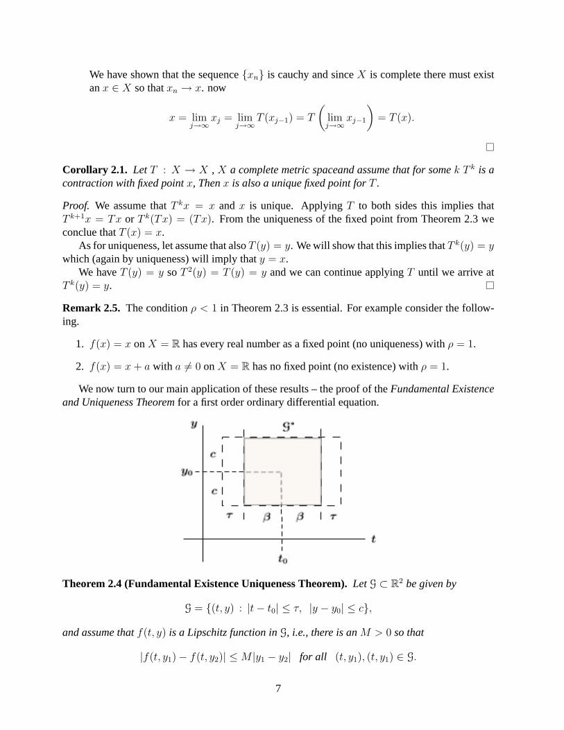
Theorem 2.4 (Fundamental Existence Uniqueness Theorem). Let G ⊂ R2 be given by
G = {(t, y) : |t− t0| ≤ τ, |y − y0| ≤ c},
and assume that f(t, y) is a Lipschitz function in G, i.e., there is an M > 0 so that
|f(t, y1)− f(t, y2)| ≤M |y1 − y2| for all (t, y1), (t, y1) ∈ G.
7
Let
p = max(t,y)∈G
|f(t, y)|, β = min
(τ,
c
p
),
and letG∗ = {(t, y) : |t− t0| ≤ β, |y − y0| ≤ c} ⊂ G.
Then the initial value problem
dy
dt= f(t, y) (2.4.4)
y(t0) = y0
has a unique solution in the interval |t− t0| < β.
Remark 2.6. The proof of this result is based on the Banach fixed point theorem and the importantfact that the problem (2.4.4) is equivalent to the integral equation
y(t) = y0 +
∫ t
t0
f(s, y(s)) ds. (2.4.5)
In the proof we will use the mapping
T (ϕ) = y0 +
∫ t
t0
f(s, ϕ(s)) ds, (2.4.6)
defined on the complete metric space
C∗ = {ϕ ∈ C[t0 − β, t0 + β] : |ϕ(t)− y0| ≤ c, for |t− t0| ≤ β}. (2.4.7)
Her we equip C∗ with the metric inherited from C[t0 − β, t0 + β], namely,
d(ϕ, ψ) = sup|t−t0|≤β
|ϕ(t)− ψ(t)|.
We use the fact that C∗ is a closed subset of the complete metric space C[t0 − β, t0 + β] andtherefore is a complete metric space. We have to show that T (C∗) ⊂ C∗. To do this we need onlyshow that for any ϕ ∈ C∗ we have
|T (ϕ)(t)− y0| ≤ c.
We have
|T (ϕ)(t)− y0| =∣∣∣∣∫ t
t0
f(s, ϕ(s)) ds
∣∣∣∣ (2.4.8)
≤∣∣∣∣∫ t
t0
|f(s, ϕ(s))| ds∣∣∣∣
≤ p|t− t0| ≤ pβ ≤ c.
8
We also claim that there exists an N so that TN is a contraction on C∗. Notice that
|T (ϕ1)(t)− T (ϕ2)(t)| =∣∣∣∣∫ t
t0
[f(s, ϕ1(s))− f(s, ϕ2(s))] ds
∣∣∣∣ (2.4.9)
≤∣∣∣∣∫ t
t0
∣∣f(s, ϕ1(s))− f(s, ϕ2(s))∣∣ ds∣∣∣∣
≤M
∣∣∣∣∫ t
t0
∣∣ϕ1(s)− ϕ2(s)∣∣ ds∣∣∣∣
≤M |t− t0| d∞(ϕ1, ϕ2) ≤M β d∞(ϕ1, ϕ2).
Since T (ϕ1), T (ϕ2) are back in C∗ we can apply T to them and again use the Lipschitz condi-tion to get
|T 2(ϕ1)(t)− T 2(ϕ2)(t)| =∣∣∣∣∫ t
t0
[f(s, T (ϕ1)(s))− f(s, T (ϕ2)(s))] ds
∣∣∣∣ (2.4.10)
≤M
∣∣∣∣∫ t
t0
∣∣T (ϕ1)(s)− T (ϕ2)(s)∣∣ ds∣∣∣∣
≤M2d∞(ϕ1, ϕ2)
∫ t
t0
|t− t0| ds ≤M2 |t− t0|22
d(ϕ1, ϕ2)
≤M2 β2
2d(ϕ1, ϕ2).
Continuing in this way we can eventually obtain
d∞(T n(ϕ1), Tn(ϕ2)) ≤
Mnβn
n!d(ϕ1, ϕ2). (2.4.11)
It is clear that we can take N sufficiently large that
MNβN
N !< 1.
Thus we can conclude that TN is a contraction on C∗.
Proof of Theorem 2.4. Let (t0, y0) ∈ G and choose β, C∗, T and N as above. Then starting withany x0 in C∗ we can obtain a sequence of successive approximations xn = TN(xn−1). Since TN isa contraction in C∗ we can conclude from Theorem 2.4 that there is a unique fixed point y solvingTN(y) = y and from Corollary 2.1 y is also the unique fixed point of T . Thus we have T (y) = yand from (2.4.5) we conclude that (2.4.4) has a unique solution.
2.5 Norms, Inner Products, Banach and Hilbert Space
In the last section we studied the basic tools of vector spaces and metric spaces. Then we intro-duced the idea of a complete metric space and fixed point methods for contraction mappings. Inthis section we put two of these ideas together – namely, we consider a distance function on avector space.
Normed Spaces
9
Definition 2.8. Let X be a vector space.
1. A norm ‖ · ‖ on X is a function from X to R+ satisfying
(a) ‖x‖ ≥ 0 and ‖x‖ = 0 if and only if x = 0.
(b) αx‖ = |α|‖x‖ for all x ∈ X and scalar α.
(c) ‖x + y‖ ≤ ‖x‖+ ‖y‖
2. A vector space with a norm is called a normed space.
Remark 2.7. 1. Every normed space is a metric space. Just define d(x, y) = ‖x− y‖.
2. The norm is a continuous function,i.e., if f(x) = ‖x‖ and xnn→∞−−−→ x, then f(xn)
n→∞−−−→f(x). To see this use the backwards triangle inequality (see the exercises)
| ‖x‖ − ‖y‖ | ≤ ‖x− y‖.
3. Let X = R and define
d(x, y) =
{0 x = y
1 x = y.
The function d is a metric but there does not exist a norm that generates this metric.
We can show this by contradiction. Suppose that ‖ · ‖ is a norm so that d(x, y) =x− y‖. Then for all α = 0, we must have ‖αx‖ = |α|‖x‖. Let α = 2 and x = 0, then
1 = ‖αx‖ = |α|‖x‖ = 2
which is a contradiction.
4. If a metric satisfies the extra condition
d(αx, αy) = |α|d(x, y), for all x, y ∈ X, α ∈ R(C),
then the ‖x‖ ≡ d(x, 0) is a norm.
Definition 2.9. A X normed space for which the associated metric induced by the norm is com-plete is called a Banch space.
Inner Product Spaces
Definition 2.10. Let X be a (real) vector space.
1. A real inner product 〈·, ·〉 is a function from X ×X to R satisfying:
(a) 〈x, y〉 = 〈y, x〉 for all x ∈ X .
(b) 〈αx, y〉 = α〈x, y〉 for all x, y ∈ X and scalar α ∈ R.
(c) 〈x + y, z〉 = 〈x, z〉+ 〈y, z〉.
10
(d) 〈x, x〉 ≥ 0 for all x ∈ X and 〈x, x〉 = 0 if and only if x = 0.
2. A vector space with a real inner product is called a real inner product space.
Definition 2.11. Let X be a (complex) vector space.
1. A complex inner product 〈·, ·〉 is a function from X ×X to C satisfying:
(a) 〈x, y〉 = 〈y, x〉 for all x ∈ X .
(b) 〈αx, y〉 = α〈x, y〉 for all x, y ∈ X and scalar α ∈ C.
(c) 〈x + y, z〉 = 〈x, z〉+ 〈y, z〉.(d) 〈x, x〉 ≥ 0 for all x ∈ X and 〈x, x〉 = 0 if and only if x = 0.
2. A vector space with a real inner product is called a complex inner product space.
Note that for a complex vector space we have
〈x, αy〉 = 〈αy, x〉 = α 〈y, x〉 = α 〈x, y〉,
and therefore
〈x, αy〉 = α 〈x, y〉. (2.5.1)
Example 2.4. 1. X = Rn is a real inner product space with 〈x, y〉 =n∑j=1
xjyj .
2. X = Cn is a complex inner product space with 〈x, y〉 =n∑j=1
xjyj .
3. L2(a, b) is a real inner product space with 〈f, g〉 =
∫ b
a
f(x) g(x) dx.
4. L2(a, b) is a complexl inner product space with 〈f, g〉 =
∫ b
a
f(x)g(x) dx.
Theorem 2.5 (Schwarz Inequality). For any x, y in a complex (or real) inner product space Xwe have
|〈x, y〉| ≤〉x, x〉〈y, y〉. (2.5.2)
Equuality holds if and only if y is a multiple of x.
Proof. First we note that for all x and w
0 ≤ 〈x− w, x− w〉 (2.5.3)
〈x, x〉 − 〈x,w〉 − 〈w, x〉+ 〈w,w〉
〈x, x〉 − 2Re (〈x,w〉) + 〈w,w〉.
11
we also note that equality holds if and only if x = w (i.e., x− w = 0). Therefore
〈x, x〉 ≥ 2Re (〈x,w〉) + 〈w,w〉. (2.5.4)
We now set
w =〈x, y〉〈y, y〉y
in (2.5.4) to obtain
〈x, x〉 ≥ 2Re
((
⟨x,〈x, y〉〈y, y〉y
⟩)+
⟨〈x, y〉〈y, y〉y,
〈x, y〉〈y, y〉y
⟩
= 2Re
[〈x, y〉〈y, y〉 〈x, y〉
]+|〈x, y〉|2〈y, y〉2 〈y, y〉
= 2|〈x, y〉|2〈y, y〉 −
|〈x, y〉|2〈y, y〉 =
|〈x, y〉|2〈y, y〉 .
Thus we have|〈x, y〉|2 ≤ 〈x, x〉 〈y, y〉.
Now recall that equality holds above if and only if x is a multiple of y (since, by definition ofw, it is a multiple of y).
Remark 2.8. Every inner product space is a norm space. To see this we define a norm by
‖x‖ = 〈x, x〉1/2. (2.5.5)
To show that this gives a norm we must show that the triangle inequality holds.
0 ≤ ‖x + y‖2 = 〈x + y, xy〉 = 〈x, 〉+ 〈x, y〉+ 〈y, x〉+ 〈y, y〉
= ‖x‖2 + 2Re 〈x, y〉+ ‖y‖2
≤ ‖x‖2 + 2|〈x, y〉|+ ‖y‖2
≤ ‖x‖2 + 2‖x‖‖y‖+ ‖y‖2
= (‖x‖+ ‖y‖)2,
and we have‖x + y‖ ≤ ‖x‖+ ‖y‖.
Lemma 2.1. The inner product in an inner product space is a continuous function in its arguments.Indeed, we have
1. If xn → x and yn → y, then 〈xn, yn〉 → 〈x, y〉 (here un → u means ‖un − u‖ → 0 where‖u‖ = 〈u, u〉.)
12
2. For every v, if xn → x then 〈xn, v〉 → 〈x, v〉.
3. If xn → x then ‖xn‖ → ‖x‖.
Lemma 2.2. The norm induced from the inner product satisfies the parallelogram law
‖x + y‖2 + ‖x− y‖2 = 2‖x‖2 + 2‖y‖2.
Hilbert Spaces
We have seen that every inner product space is a norm space. If in addition the norm is completethen it is a Banach space. But in this case we use a different name in honor of David Hilbert.
Definition 2.12. An inner product space for which the induced norm gives a complete metric spaceis called a Hilbert space.
Definition 2.13. 1. Two vectors x and y in X are orthogonal if 〈x, y〉 = 0.
2. A subset S ⊂ X is an orthogonal set if each pair of elements of S are orhtogonal.
3. A set is orthonormal if it is orthogonal and every element x ∈ S satisfies ‖x‖ = 1.
Remark 2.9. If 〈x, y〉 = 0 then the parallelogram law reduces to the Pythagorean Theorem
‖x− y‖2 = ‖x‖2 + ‖y‖2 and ‖x + y‖2 = ‖x‖2 + ‖y‖2.
By definition, a Hilbert space H is a vector space, so that a subset M ⊂ H is a subspace ifαx+βy ∈M for all x, y ∈M and scalars α and β. Thus if x0 ∈ H , then M = {αx0} = Span{x0}is a subspace.
Definition 2.14. The (orthogonal) projection of x ∈ H on M = Span{x0} is defined by
Px =〈x, x0〉‖x0‖2
x0.
Note that the following properties of P hold.
1. P 2 = P . Namely we have
P 2x = P (Px) =〈Px, x0〉‖x0‖2
x0 = 〈x, x0〉〈x0, x0〉‖x0‖2
x0
‖x0‖2= Px.
13
2. 〈Px, y〉 = 〈x, Py〉. To see this we note that
〈Px, y〉 =
⟨〈x, x0〉‖x0‖2
x0, y
⟩
=〈x, x0〉‖x0‖2
〈x0, y〉
=〈x, x0〉‖x0‖2
〈y, x0〉
=
⟨x,〈y, x0〉‖x0‖2
y
⟩= 〈x, Py〉.
3. 〈Px, (I − P )y〉 = 0 since
〈Px, (I − P )y〉 = 〈Px, y〉 − 〈Px, Py〉= 〈Px, y〉 − 〈P 2x, y〉= 〈Px, y〉 − 〈Px, y〉= 0.
4. For every x ∈ H we have x = Px + (I − P )x and Px ⊥ (I − P )x.
Definition 2.15. 1. Given x and y in a Hilbert space H we define the angle θ between x and yby the formula
cos(θ) =〈x, y〉‖x‖ ‖y‖ .
2. If M ↪→ H (a subspace) is a closed subspace if {xn} ⊂ M and xn → x ∈ H implies thatx ∈M .
3. If M ⊂ H the the orthogonal complement of M , denoted M⊥ is the subspace
M⊥ = {x ∈ H : 〈x,m〉 = 0 for all m ∈M}.
4. M⊥ is a closed subspace of H
If {xn} ⊂M⊥ and xn → x then
〈x,m〉 = limn→∞〈xn,m〉 = 0, for all m ∈M,
so 〈x,m〉 = 0 for all m ∈M and x ∈M⊥.
14
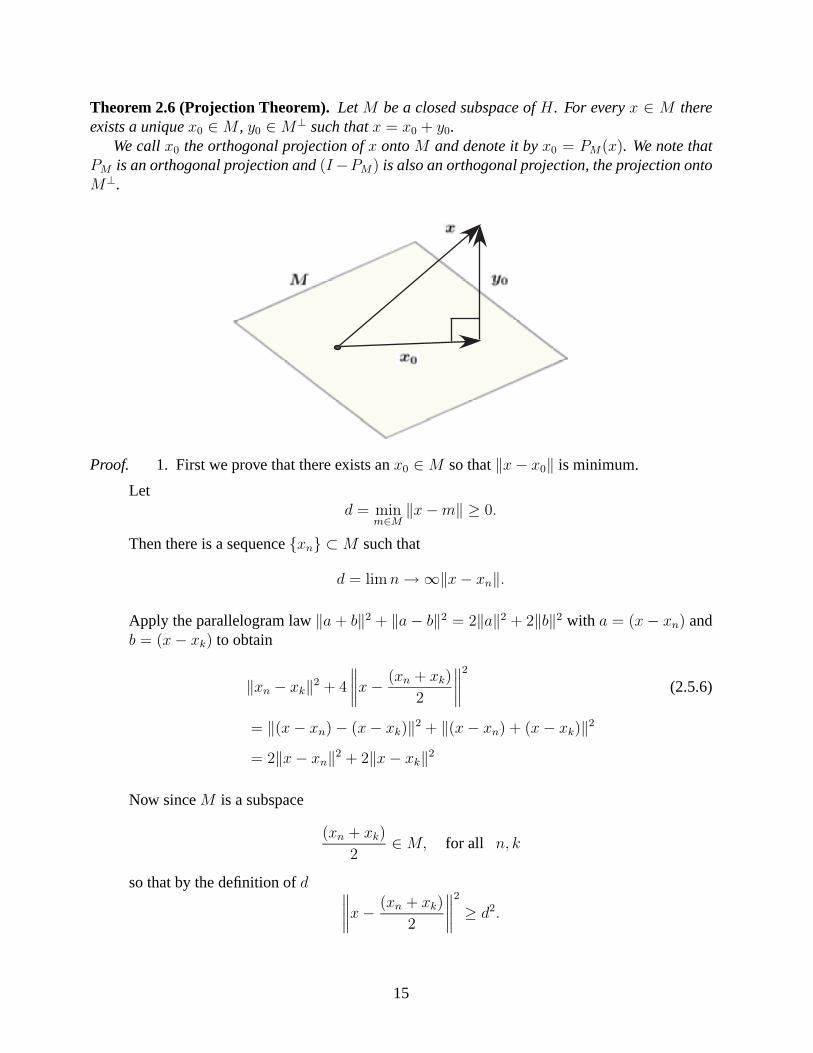
Theorem 2.6 (Projection Theorem). Let M be a closed subspace of H . For every x ∈ M thereexists a unique x0 ∈M , y0 ∈M⊥ such that x = x0 + y0.
We call x0 the orthogonal projection of x onto M and denote it by x0 = PM(x). We note thatPM is an orthogonal projection and (I−PM) is also an orthogonal projection, the projection ontoM⊥.
Proof. 1. First we prove that there exists an x0 ∈M so that ‖x− x0‖ is minimum.
Letd = min
m∈M‖x−m‖ ≥ 0.
Then there is a sequence {xn} ⊂M such that
d = limn→∞‖x− xn‖.
Apply the parallelogram law ‖a + b‖2 + ‖a− b‖2 = 2‖a‖2 + 2‖b‖2 with a = (x− xn) andb = (x− xk) to obtain
‖xn − xk‖2 + 4
∥∥∥∥x− (xn + xk)
2
∥∥∥∥2
(2.5.6)
= ‖(x− xn)− (x− xk)‖2 + ‖(x− xn) + (x− xk)‖2
= 2‖x− xn‖2 + 2‖x− xk‖2
Now since M is a subspace
(xn + xk)
2∈M, for all n, k
so that by the definition of d ∥∥∥∥x− (xn + xk)
2
∥∥∥∥2
≥ d2.
15
Therefore from (2.5.6) we have
‖xn − xk‖2 ≤ 2‖x− xn‖2 + 2‖x− xk‖2 − 4d2
→ 2d2 + 2d2 − 4d2 = 0 as n, k →∞.
We conclude that the sequence {xn} is Cauchy and since H is a Hilbert space (and hencecomplete), there exists an x0 ∈ H so that xn → x. Finally since M is closed and {xn} ⊂Mwe must have x0 ∈M and
‖x− x0‖ = limn→∞
‖x− xn‖ = d.
2. Let w = (x − x0). We show that x ⊥ M , i.e. 〈w,m〉 = 0 for all m ∈ M . This is clearlytrue for m = 0 so let us assume that m = 0. Note that x0 − αm ∈ M for all α ∈ R(C) andm ∈M (since M is a vector space). So we have
‖w − αm‖2 = ‖x− (x0 + αm)‖2≥ ‖x− x0‖2 = ‖w‖2.
From this we see that the real valued function f(α) = ‖w−αm‖2 has a minimum at α = 0.Now let use write f is another way
f(α) = 〈w − αm,w − αm〉= ‖w‖2 + α2‖m‖2 − α〈w,m〉 − α〈m,w〉.
Take the derivative with respect to α and set α = 0. Since α = 0 is a minumum this resultmust be zero:
f ′(α)∣∣α=0
=[2α‖m‖2 − 2Re (〈w,m〉)
]∣∣α=0
= 2Re (〈w,m〉) = 0, for all m ∈M.
Now if this is a real Hilbert space then 〈w,m〉 = Re (〈w,m〉) = 0 and we are done, other-wise, if H is a complex Hilbert space then im ∈ H for every m ∈ H so we can write
Re (〈w, im〉 = 0, fpr all m ∈M.
This implies
0 = Re [−i〈w,m〉]= Re [−i(Re 〈w,m〉+ i〈w,m〉)]= Im 〈w,m〉
so we have Im 〈w,m〉 = 0 for all m ∈ M and finally we conclude that 〈w,m〉 = 0 for allm ∈M .
3. At this point we have shown that for every x ∈ H there exists an x0 ∈M and w = x− x0 ∈M⊥. It is clear that if we let y0 = (x − x0) ∈ M⊥ then x = x0 + y0 gives the desired
16
decomposition. Our final goal is to show that this decomposition is unique. To this end letus suppose that also x = x0 + y0 with x0 ∈M and y0 ∈M⊥. Then we can write
0 = x− x = (x0 − x0)− (y0 − y0)
where (x0− x0) ∈M and (y0− y0) ∈M⊥. If we take the inner product of 0 = (x0− x0)−(y0− y0), first with (x0− x0) and then with (y0− y0) (and use the fact that 〈(x0− x0), (y0−y0)〉 = 0) we have
‖(x0 − x0)‖0 = 0, ‖(y0 − y0)‖0 = 0,
and we conclude that x0 = x0 and y0 = y0.
Exercises for Chapter 2
1. Show that the subset P0n = {p(x) ∈ Pn : p(0) = 0} is a subspace of P. Find its dimension.
Find a basis.
2. Show that the subset Qn = {p(x) ∈ Pn : p(0) = 1} is not a vector space.
3. Consider the ordinary differential equation y′′ = 0 on 0 < x < 1. Find the dimension of thevector space of all solutions satisfying:
(a) y(0) = y(1)
(b) y(0) = y(1) = 0
(c) y′(0) = y′(1) = 0
4. Let C∗ be the set of all real-valued continuous functions on R such that the derivative doesnot exist at x = 0. Is C∗ a vector space?
5. Given vectors x1 = (1,−1, 0), x2 = (2, 1,−1), x3 = (0, 1, 1), x4 = (0, 3,−1). Are x1, x2,x3 linearly independent or dependent? Same question for x1, x2, x4? Give reasons for youranswers, i.e., show why your answer is correct.
6. Show that the continuous functions on an interval [a, b], denoted C[a, b], is a metric spacewith the distqance function d(f, g) = sup
x∈[a,b]
|f(x)− g(x)|.
7. Let L2(−1, 1) denote the space C[−1, 1] with the metric function
d2(f, g) =
(∫ 1
−1
|f(x)− g(x)|2 dx)1/2
.
17
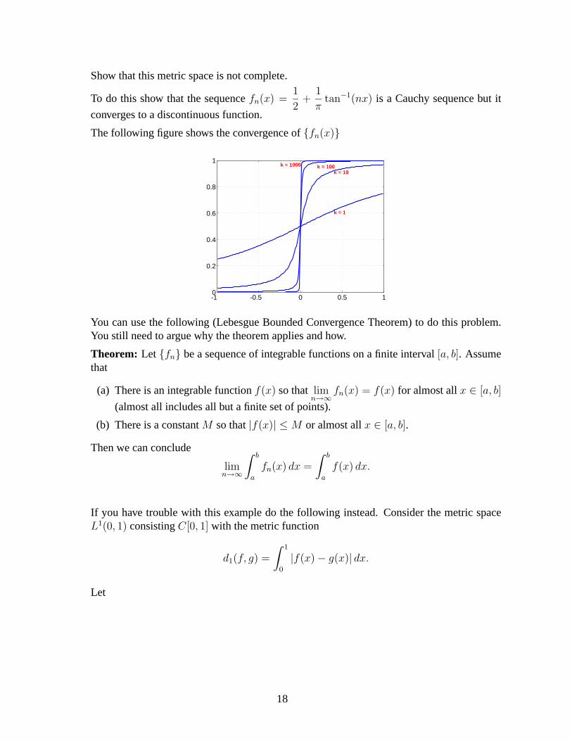
Show that this metric space is not complete.
To do this show that the sequence fn(x) =1
2+
1
πtan−1(nx) is a Cauchy sequence but it
converges to a discontinuous function.
The following figure shows the convergence of {fn(x)}
-1 -0.5 0 0.5 10
0.2
0.4
0.6
0.8
1
k = 1
k = 10k = 100k = 1000
You can use the following (Lebesgue Bounded Convergence Theorem) to do this problem.You still need to argue why the theorem applies and how.
Theorem: Let {fn} be a sequence of integrable functions on a finite interval [a, b]. Assumethat
(a) There is an integrable function f(x) so that limn→∞
fn(x) = f(x) for almost all x ∈ [a, b]
(almost all includes all but a finite set of points).
(b) There is a constant M so that |f(x)| ≤M or almost all x ∈ [a, b].
Then we can conclude
limn→∞
∫ b
a
fn(x) dx =
∫ b
a
f(x) dx.
If you have trouble with this example do the following instead. Consider the metric spaceL1(0, 1) consisting C[0, 1] with the metric function
d1(f, g) =
∫ 1
0
|f(x)− g(x)| dx.
Let
18
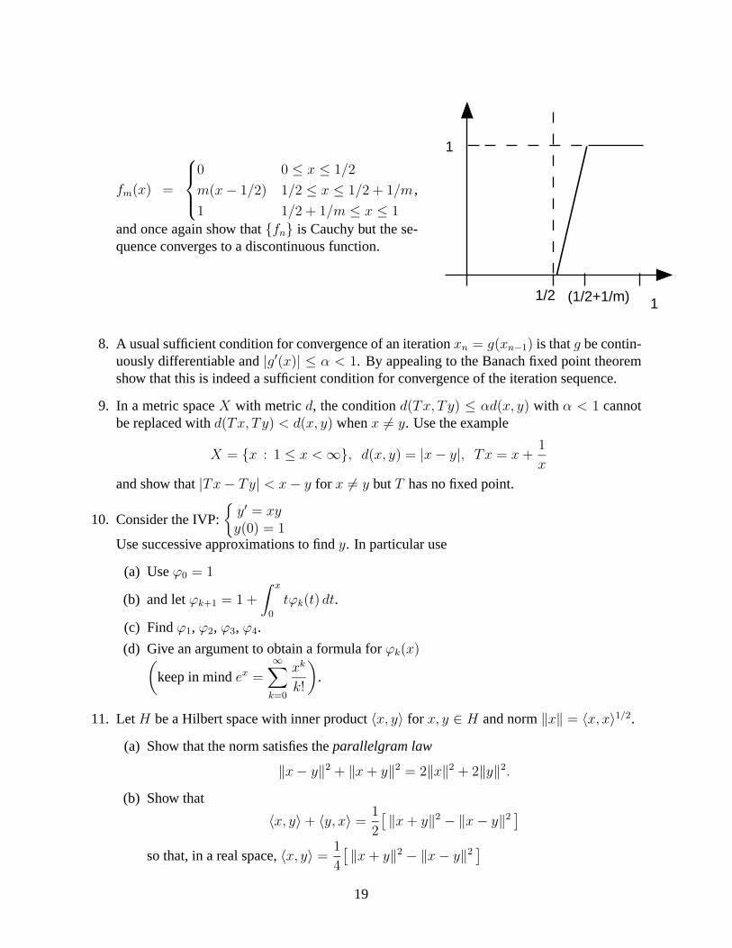
fm(x) =
0 0 ≤ x ≤ 1/2
m(x− 1/2) 1/2 ≤ x ≤ 1/2 + 1/m
1 1/2 + 1/m ≤ x ≤ 1
,
and once again show that {fn} is Cauchy but the se-quence converges to a discontinuous function.
1
1/21(1/2+1/m)
8. A usual sufficient condition for convergence of an iteration xn = g(xn−1) is that g be contin-uously differentiable and |g′(x)| ≤ α < 1. By appealing to the Banach fixed point theoremshow that this is indeed a sufficient condition for convergence of the iteration sequence.
9. In a metric space X with metric d, the condition d(Tx, Ty) ≤ αd(x, y) with α < 1 cannotbe replaced with d(Tx, Ty) < d(x, y) when x = y. Use the example
X = {x : 1 ≤ x <∞}, d(x, y) = |x− y|, Tx = x +1
x
and show that |Tx− Ty| < x− y for x = y but T has no fixed point.
10. Consider the IVP:
{y′ = xyy(0) = 1
Use successive approximations to find y. In particular use
(a) Use ϕ0 = 1
(b) and let ϕk+1 = 1 +
∫ x
0
tϕk(t) dt.
(c) Find ϕ1, ϕ2, ϕ3, ϕ4.
(d) Give an argument to obtain a formula for ϕk(x)(keep in mind ex =
∞∑k=0
xk
k!
).
11. Let H be a Hilbert space with inner product 〈x, y〉 for x, y ∈ H and norm ‖x‖ = 〈x, x〉1/2.
(a) Show that the norm satisfies the parallelgram law
‖x− y‖2 + ‖x + y‖2 = 2‖x‖2 + 2‖y‖2.
(b) Show that
〈x, y〉+ 〈y, x〉 =1
2
[‖x + y‖2 − ‖x− y‖2
]so that, in a real space, 〈x, y〉 =
1
4
[‖x + y‖2 − ‖x− y‖2
]19
(c) Show that in a complex Hilbert space
〈x, y〉 − 〈y, x〉 =i
2
[‖x + iy‖2 − ‖x− iy‖2
].
(d) Consequently, in a complex Hilbert space
〈x, y〉 =1
4
[‖x + y‖2 − ‖x− y‖2 + i‖x + iy‖2 − i‖x− iy‖2
]12. Show that the reverse triangle inequality holds in any normed space, i.e.,∣∣ ‖x‖ − ‖y‖ ∣∣ ≤ ‖x− y‖.
13. For the numerical example of collocation using Maple modify the Maple code to use thedifferent points x1 = 1/4 and x2 = 3/4.
14. Use the Maple code to carry out the Taylor method for F (x, y) = 3x2y,y(0) = 1 on [0, 1].
15. Use the Maple euler_solve procedure to approximate the solution ofy′ = t2 − y on [0, 2] with y(0) = 1. The exact answer is y = −e−t + t2 − 2t + 2. Useh = .2, .1, .05.
References
[1] L. Collatz, “The numerical treatment of Differential Operators,” Springer-Verlag, NY, 1966.
[2] V.I. Arnol’d, “Ordinary differential equations,” Springer-textbook, Springer-Verlag, 1992.
[3] “Differential Equations,” Frank Ayres, jr., Schaum’s Outline Series, Schaum Publishing, NewYork, 1952.
[4] F. Brauer, J.A. Nohel, Qualitative Theory of Ordinary Differential Equtions, Dover, 1969.
[5] E.A. Coddington and N. Levinson, “Theory of Ordinary Differential Equations,” McGraw-Hill Book Co. New York, Toronto, London (1955).
[6] E.A. Coddington, “An introduction to ordinary differential equations,” Dover 1989.
[7] G.F. Simmons, “Differential Equations with applications and historical notes,” McGraw-HillBook Co. New York, Toronto, London (1972).
[8] H. Sagan, “Boundary and Eigenvalue Problems in Mathematical Physics,” J. Wiley & Sons,Inc, New York, 1961.
[9] D.A. Sanchez, Ordinay Differential Equations and Stability Theory: An Introduction, W.H.Freeman and Company, 1968.
20
[10] I. Stakgold, “Green’s Functions and Boundary Value Problems,” Wiley-Interscience, 1979.
[11] R. Dautray and J.L. Lions, Mathematical analysis and numerical methods for science andtechnology,
[12] J. Dieudonne, Foundations of Modern Analysis, Academic press, 1960.
[13] S. J. Farlow, “Partial differential equations for scientists and engineers, Dover 1993.
[14] G. Folland, Introduction to partial differential equations,
[15] G. Folland, Fourier Series and its Applications, Brooks-Cole Publ. Co., 1992.
[16] K.E. Gustafson Partial differential equations,
[17] R.B. Guenther and J.W. Lee, Partial Differential Equations of Mathematical Physics andIntegral Equations, (Prentice Hall 1988), (Dover 1996).
[18] G. Hellwig, Partial differential equations, New York, Blaisdell Publ. Co. 1964.
[19] J. Kevorkian, Partial differential equations,
[20] M. Pinsky, Introduction to partial differential equations with applications,
[21] W. Rudin, Functional analysis, McGraw-Hill, New york, 1973.
[22] H.F. Weinberger, Partial differential equations, Waltham, Mass., Blaisdel Publ. Co., 1965.
[23] E.C. Zachmanoglou and D.W. Thoe, Introduction to partial differential equations with appli-cations,
[24] Richard L. Burden, J. Douglas Faires and Albert C. Reynolds, “Numerical Analysis,” Prindle,Weber and Schmidt, Boston, 1978.
[25] G. Dahlquist and A. Bjorck, “Numerical Methods,” Prentice-Hall Series in Automatic Com-putation, Englewood, NJ, 1974.
[26] Kendall E. Atkinson, “An Introduction to Numerical Analysis,” John Wiley and Sons, 1978.
[27] John H. Mathews, “Numerical Methods: for computer science, engineering amd mathemat-ics,” 2nd Ed, 1992 Prentice Hall, Englewood Cliffs, New Jersey, 07632, U.S.A.
[28] M. Razzaghi and M. Razzaghi, “Solution of linear two-point boundary value problems viaTaylor series,” J. Franklin Inst., 326, No. 4, 1989, 511-521.
21