Embed Size (px)
Citation preview

Intro to Macroeconomics
1. Gross domestic product2. The business cycle3. The U.S. economic record4. Aggregate demand curve5. Aggregate supply curve6. Equilibrium GDP and price level

Keynesian revolutionJohn Maynard Keynes. The General Theory of Employment, Interest, and Money, 1936.
The macroeconomic problem: Persistent underutilization of resources or “poverty in the midst of plenty.”

Stocks versus flowsStock variables are cumulated values measured at a specific point in time.
Examples: Bank balances, debt, inventories.
Flow variables are measured per unit point in time.
Examples: Income (including profits), output.
Gross domestic product (GDP)The market value of new goods and services produced within the nation’s border within one year.
GDP is our basic measure of aggregate (total) economic activity

The business cycleWave-like movement of aggregate economic activity over time.
• Business cycles are irregularly recurring• A full cycle consists of an expansion and a
contraction (recession).
7
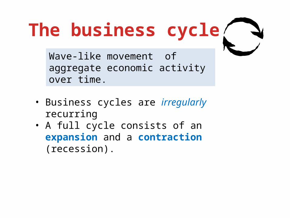
Hypothetical business cycles
8
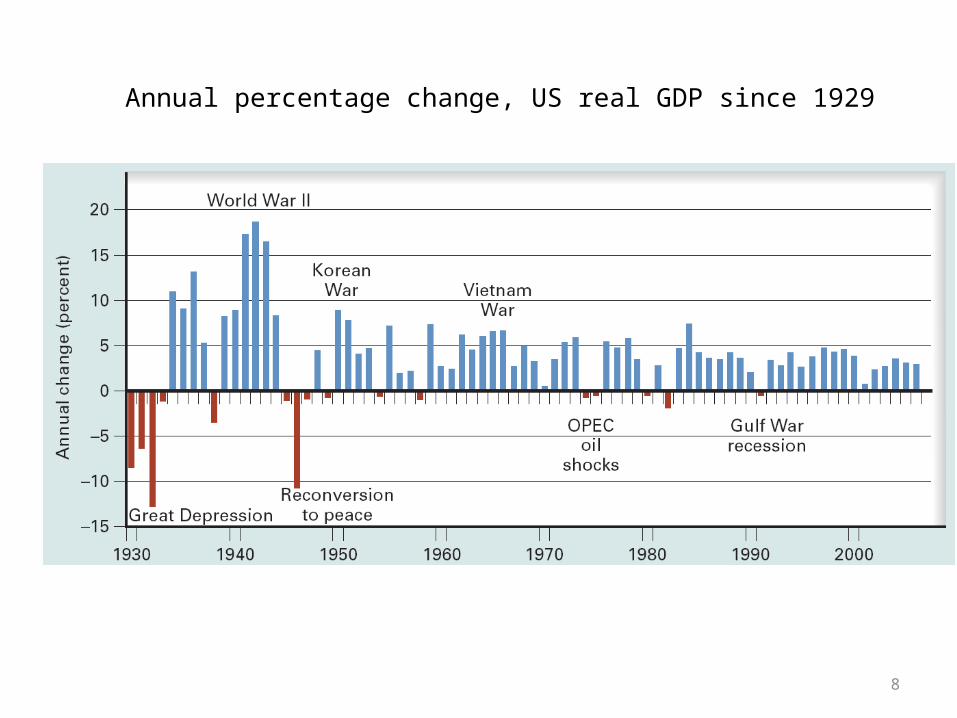
Annual percentage change, US real GDP since 1929

9
US and UK annual growth rates in output are similar
10
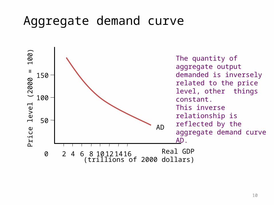
Aggregate demand curve
Real GDP (trillions of 2000 dollars)
0 2 4 6 8 10 12 14 16
50
150
100
Pric
e le
vel (
2000
= 1
00)
AD
The quantity of aggregate output demanded is inversely related to the price level, other things constant.This inverse relationship is reflected by the aggregate demand curve AD.

Real balance (Wealth) effectLet M denote money balances and P is the price level. Real money balances (RB) are given by:
P
MRB
As the price level rises, my money loses its buying power. Thus I will buy
less.
Real GDP
Pric
e Le
vel
0
AS
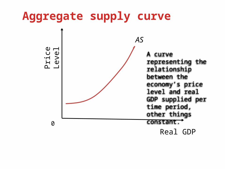
Aggregate supply curve
A curve representing the relationship between the economy’s price level and real GDP supplied per time period, other things constant.
13
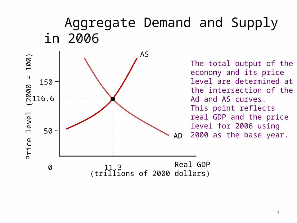
Aggregate Demand and Supply in 2006
Real GDP (trillions of 2000 dollars)
0 11.3
50
150
116.6
Pric
e le
vel (
2000
= 1
00)
AD
ASThe total output of the economy and its price level are determined at the intersection of the Ad and AS curves.This point reflects real GDP and the price level for 2006 using 2000 as the base year.
14
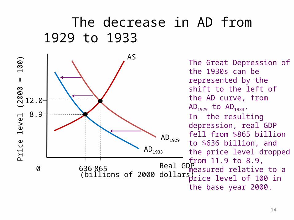
The decrease in AD from 1929 to 1933
8.9
12.0
Pric
e le
vel (
2000
= 1
00)
AD1929
AS
Real GDP (billions of 2000 dollars)
0 865636
AD1933
The Great Depression of the 1930s can be represented by the shift to the left of the AD curve, from AD1929 to AD1933. In the resulting depression, real GDP fell from $865 billion to $636 billion, and the price level dropped from 11.9 to 8.9, measured relative to a price level of 100 in the base year 2000.
Stagflation
•Word is a conflation of “stagnation” and “inflation.”•Stagnation means stagnant or negative growth of output and jobs.•Inflations means a sustained increase in the cost-of-living.
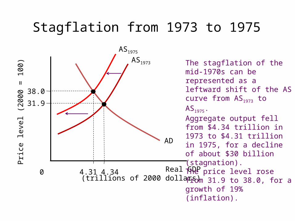
Stagflation from 1973 to 1975
38.0
31.9
Pric
e le
vel (
2000
= 1
00)
AD
AS1973
Real GDP (trillions of 2000 dollars)
0 4.344.31
AS1975
The stagflation of the mid-1970s can be represented as a leftward shift of the AS curve from AS1973 to AS1975. Aggregate output fell from $4.34 trillion in 1973 to $4.31 trillion in 1975, for a decline of about $30 billion (stagnation). The price level rose from 31.9 to 38.0, for a growth of 19% (inflation).
17
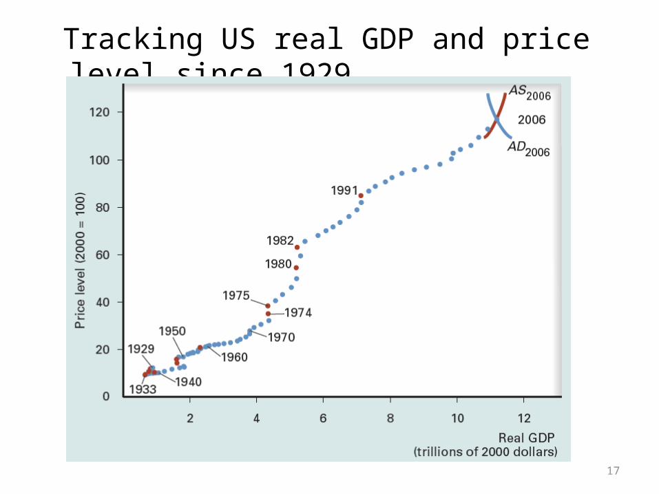
Tracking US real GDP and price level since 1929