1997 Hawaii Fishery Input-Output Model and Methodology

Aaron Peterson SMS Research and

Marketing Services, Inc. 1042 Fort Street Mall, Suite 200

Honolulu, HI 96813

SOEST 05-02 JIMAR Contribution 05-356

2

ACKNOWLEDGMENTS This project was conducted by SMS Research and Marketing Services, Inc. The author thanks Minling Pan, Economist of the Pacific Islands Fisheries Science Center, National Marine Fisheries Service, for her assistance and consultation throughout the project. This project and report were funded by cooperative agreement #658326 between the Joint Institute of Marine and Atmospheric Research (JIMAR) and the National Oceanic and Atmospheric Administration (NOAA). The views expressed herein are those of the authors and do not necessarily reflect the view of NOAA or any of its subdivisions.

3

Table of Contents 1. BACKGROUND .......................................................................................................................................5 2. OBJECTIVES ...........................................................................................................................................5 3. DIFFERENCES AND IMPROVEMENTS IN THIS MODEL .........................................................6 4. CHANGES IN THE FISHERY INDUSTRY .......................................................................................6 5. A BRIEF DESCRIPTION OF INPUT-OUTPUT MODELING FOR FISHERIES ......................7 6. TRANSACTION TABLE ........................................................................................................................9 7. MARGINS................................................................................................................................................12 8. FISHERY SALES ...................................................................................................................................13 9. MULTIPLIERS.......................................................................................................................................16 9.1 Type I Multipliers ..............................................................................................................................17 9.2 Type II Multipliers.............................................................................................................................17 10. CONCLUSIONS .....................................................................................................................................18 11. REFERENCES ........................................................................................................................................19 APPENDIX ..............................................................................................................................................20 Data Sources..............................................................................................................................................20 Methodology .............................................................................................................................................20 Commercial Longline............................................................................................................................20 Small Commercial Boats ......................................................................................................................21 Expense/Recreational Boats .................................................................................................................21 Charter Boats ........................................................................................................................................22 Visitor Expenditure, Charter Boats .....................................................................................................23 Sales of Commercial Fishing Industries..................................................................................................23 Transactions Table ....................................................................................................................................23 Recommendations for the Future.............................................................................................................24 Detailed Methodology on Building Longline Production Functions ....................................................24

4

5

1. BACKGROUND The fisheries industry in Hawaii has gone through some major changes in recent years. At the forefront of this were the restrictions on commercial longline swordfish fishing around Hawaiian waters. The courts considered the impact of this industry on endangered species, namely the leatherback turtle, devastating. The restrictions on longline swordfish fishing was in effect for several years but recently the federal court chose to lift the ban, but places the fisheries under certain restrictions. Given the visibility of the court ruling, the fishery industry has undergone increased scrutiny in terms of research, both environmental and economic. In order to conduct economic research on the fisheries industry in Hawaii, the tools needed must be current and available. The major tool used to do economic research is the fishery input-output model. The first fishery input-output model was built for the year 1992, and this report presents the updated 1997 fishery input-output model, with additional fishery sectors. The latest year that sufficient data were available to build an input-output model for Hawaii was 1997. The fishery model is based on the 1997 Hawaii State Input-Output Model, with additional detail and attention given to the fishery sectors. 2. OBJECTIVES The major objective of creating an input-output model is to understand the linkages between the different sectors and groups that make up an economy. Understanding these linkages help economists analyze how changes in one part of an economy affect the rest of the economy. This study was undertaken to update the previous Hawaii Fishery Input-Output Model. The 1997 model updates the previous model and also includes additional fishery sectors. This report was not written to be an academic treatment of Fishery Input-Output modeling and assumes a general understanding of input-output modeling. The purpose of this report is to provide an understanding of the tools and methods that go into and come out of an input-output model. The main focus of this report is on understanding and using this model for real-world analysis, and also on the preliminary components that go into building the input-output model because they are often just as valuable as the finished model. The appendix contains the detailed methodology used to build the model. A more in-depth discussion on the general concepts of input-output modeling is available from Hawaii State Department of Business, Economic Development, and Tourism (DBEDT [Department of Business, Economic Development, and Tourism, 2003; www3.hawaii.gov/DBEDT]) or the U.S. Bureau of Economic Analysis (BEA [Bureau of Economic Analysis, 1998; www.bea.gov]). Both organizations have websites that provide very good descriptions of input-output modeling.

6

3. DIFFERENCES AND IMPROVEMENTS IN THIS MODEL The 1992 Fishery Input-Output Model was originally based on the 1992 Hawaii State Input-Output Model and expanded to include four fishery sectors. The fishery industry was broken down into more detail for the 1997 update of the Hawaii Fishery Input-Output Model. The previous version in 1992 had four fishery industries. • Longline • Small boat • Recreation and expense boats • Charter fishing The 1997 model has six industries. • Tuna longline • Swordfish longline • Commercial small boats • Recreation boats • Expense boats • Charter boats In addition, the 1997 Fishery Input-Output Model has a separate visitor expenditure vector for visitors that come to Hawaii for charter fishing. 4. CHANGES IN THE FISHERY INDUSTRY The 1997 Fishery Input-Output Model has more detail than the previous model. Table 1 shows some of the basic economic data that went into building the models. In order to show comparability between models, the data were combined in certain sectors. Table 1 presents the output and jobs for 1992 and 1997 by fishery sector. Table 1. Output and jobs by fishery sector, 1997 and 1992.

Output Wage and

Salary Jobs Proprietors Jobs 1997 1992 1997 1992 1997 1992

Swordfish longline 22.7 116 102 Tuna longline 27.4 215 191 Total Longline 50.0 43.9 331 120 299 532 Small commercial boats 11.7 13.9 10 40 507 317 Expense boats 3.9 1002 Recreation boats 10.3 0 Recreational & expense boats 14.2 23.9 0 0 1002 0 Charter boats 14.2 16.5 175 325 67 92 Note: The 1997 model provides more detailed industries than the 1992 model. The items in bold were created to provide a comparison between 1992 and 1997.

7

It is interesting to note that although the total jobs for longline have not changed much, the distribution of jobs between wage and salary and proprietors has changed. The data for these jobs comes from the BEA personal income series (BEA, SA-05, 2001; SA-07, 2001; SA-25, 2001; SA-27, 2001). One significant change between 1992 and 1997 is the number of jobs in the expense boat sector. In the previous model it was assumed that no jobs existed in that sector. However, on examining the data and reviewing how BEA puts job information together it became clear that the majority of proprietors’ jobs in the commercial fishing sector were expense fishermen. Even though they just fish to cover their expenses, they do in fact have income and expenses reported to the IRS (they usually report an operating loss), and that IRS data are the source that BEA uses to determine how many proprietors’ jobs there are in the industry. 5. A BRIEF DESCRIPTION OF INPUT-OUTPUT MODELING FOR FISHERIES An input-output model is a detailed accounting of the purchases of goods and services between the industries, households, and governments that make up an economy. The concepts of input-output will not be discussed in detail in this report because it is assumed that the reader is already familiar with the concepts involved. Instead, this report will explain basic input-output concepts in brief and tie them in with specific results and outputs that come from the Fishery Input-Output Model. A more detailed report on input-output models is available from the Hawaii State DBEDT website or the various input-output online resources and documentation from the U.S. BEA. The 1997 Hawaii Fishery Input-Output Model was based on the 1997 Hawaii State Input-Output Model. The State model featured only one commercial fishing sector. In building the Fishery Model that sector was broken down into tuna longline, swordfish longline, small commercial boats, and expense boats. The charter boat fishing sector was included in the sightseeing transportation sector in the State model and was separated out in the Fishery model. Recreation boats were listed under personal consumption expenditures (PCE) in the State model and were also separated out in the Fishery model. The industries are summarized in Table 2. Table 2. Fishery sector NAICS codes and input-output industry assignments.

Industry NAICS SIC

Longline (including swordfish and tuna) 114 0912

Small commercial boats 114 0912

Expense boats 114 0912

Recreational boats Part of PCE Part of PCE

Charter boats Part of 487210 Part of 7999

An input-output model in general consists of several parts: an inter-industry matrix, which shows the purchases of goods and services between the different industries in the

8

economy; a final demand section, which shows the purchases of goods and services by final consumers, i.e., households, governments, investment, and exports; and a value added section, which shows the wages earned, taxes, and other capital costs associated with production. In the inter-industry matrix, the rows consist of the sales of an industry to other industries, and the columns refer to the purchases of one industry from other industries. The final demand columns show the purchases of the final demand sector from the individual industries. The value added section shows the amount of resources (labor, capital, etc.) that each industry uses. Table 3 gives an overview of the industries used in building the Fisheries Input-Output Model. The condensed State Input-Output Table was used as a base, and then the extra fishery sectors were added in.

Table 3. Size of fishery industry in relation to Hawaii economy. Industry Output ($million) % of Economy Swordfish longline 22.67 0.04% Tuna longline 27.37 0.05% Small commercial boats 11.70 0.02% Expense boats 3.94 0.01% Recreation boats 10.30 0.02% Charter boats 14.17 0.02% Total fishery sectors 90.15 0.15% Agriculture 753.75 1.28% Mining and construction 3,524.30 6.01% Food processing 1,054.46 1.80% Other manufacturing 2,361.95 4.03% Transportation 3,571.67 6.09% Information 1,940.25 3.31% Utilities 1,220.30 2.08% Wholesale trade 1,939.03 3.31% Retail trade 4,179.50 7.12% Finance and insurance 3,635.67 6.20% Real estate and rentals 9,412.64 16.05% Professional services 2,166.87 3.69% Business services 1,422.59 2.43% Educational services 477.47 0.81% Health services 3,859.30 6.58% Arts and entertainment 770.31 1.31% Hotels 3,456.35 5.89% Eating and drinking 2,274.74 3.88% Other services 1,671.37 2.85% Government 8,877.36 15.13% Total 58,660.04 100.00%

9

Table 4 lists the components of Gross State Product that are in the input-output table. This is the same as the State model with the addition of a visitor expenditures sector for charter boat patrons. Table 4. Final demand sectors and related fishery expenditures.

Final Demand Sector Value Value of purchases from fishery sectors

% from fishery sectors

PCE 25,226.1 34.77 0.14% VE Charter Boat 120.5 13.60 11.29% Visitor's expenditures 10,619.5 2.38 0.02% Change in inventories 62.8 - - Gross private investment 3,437.9 - - State and local govt. investment 921.5 - - State and local govt. consumption 3,663.3 0.20 0.01% Federal military consumption 5,088.0 - - Federal military investment 296.0 - - Federal civilian consumption 478.6 - - Federal civilian investment 16.7 - - Exports 2,802.3 25.36 0.90% 6. TRANSACTION TABLE The transaction table is the standard format that an input-output table is usually displayed in. The transaction table displays the industries, final demand sectors, and value added sectors in rows and columns, where the sales of industries to other industries are displayed in rows and the purchases of industries are displayed in columns. A full transaction table appears in the Appendix of this report. Tables 5 and 6 show the portions of the transaction table related to the fishery sectors. Table 5 shows the purchases of the industries, and Table 6 shows the sales of the industries. Note that the data in Table 6 is normally shown in rows instead of columns, but is transposed here to fit on one page.

10

Table 5. Fishery purchases (columns) in the transaction table (in $million).

Swordfish longline

Tuna longline

Small commercial

boats Expense

boats Recreation

boats Charter

boats Swordfish longline 0.00 0.00 0.00 0.00 0.00 0.00 Tuna longline 0.00 0.00 0.00 0.00 0.00 0.00 Small commercial boats 0.00 0.00 0.00 0.00 0.00 0.00 Expense boats 0.00 0.00 0.00 0.00 0.00 0.00 Recreation boats 0.00 0.00 0.00 0.00 0.00 0.00 Charter boats 0.00 0.00 0.00 0.00 0.00 0.00 Agriculture 0.00 0.00 0.00 0.00 0.00 0.00 Mining and construction 0.00 0.00 0.00 0.00 0.00 0.00 Food processing 0.22 0.71 0.42 0.33 0.72 0.22 Other manufacturing 1.76 1.37 1.24 1.23 2.95 1.47 Transportation 0.33 0.26 0.14 0.12 0.31 1.18 Information 0.00 0.00 0.00 0.00 0.00 0.17 Utilities 0.00 0.00 0.00 0.00 0.00 0.00 Wholesale trade 3.61 3.33 1.54 0.80 1.07 0.26 Retail trade 0.12 0.21 0.09 0.09 0.23 0.03 Finance and insurance 0.27 0.37 0.13 0.19 0.58 0.85 Real estate and rentals 0.00 0.00 0.00 0.00 0.00 0.00 Professional services 0.00 0.00 0.00 0.00 0.00 0.00 Business services 0.16 0.16 0.04 0.07 0.13 0.39 Educational services 0.00 0.00 0.00 0.00 0.00 0.00 Health services 0.00 0.00 0.00 0.00 0.00 0.00 Arts and entertainment 0.00 0.00 0.00 0.00 0.00 0.14 Hotels 0.00 0.00 0.00 0.00 0.00 0.54 Eating and drinking 0.00 0.00 0.00 0.00 0.00 0.04 Other services 1.05 1.94 0.71 0.82 2.51 0.00 Government 0.07 0.19 0.03 0.05 0.19 0.00 Intermediate demand 7.58 8.53 4.34 3.69 8.69 5.31 Imports 3.84 2.38 0.81 0.56 1.61 0.47 Compensation of employees 4.15 7.30 0.29 0.00 0.00 4.67 Proprietor's income 1.45 2.49 5.40 -0.78 0.00 1.42 Indirect business taxes 0.39 0.47 0.20 0.07 0.00 0.57 Other capital costs 5.25 6.21 0.65 0.40 0.00 1.73 Value added 11.24 16.46 6.55 -0.32 0.00 8.39 Output 22.67 27.37 11.70 3.94 10.30 14.17 Wage and salary jobs 116 215 10 0 0 175 Proprietor's jobs 102 191 507 1,008 0 67 Total jobs 218 406 517 1,008 0 242

11

Table 6. Fishery sales (rows) in transaction table (transposed, in $million).

Swordfish Longline

Tuna Longline

Small Commercial

Boats

Expense Boats

Recreation Boats

Charter Boats

Swordfish longline 0.00 0.00 0.00 0.00 0.00 0.00 Tuna longline 0.00 0.00 0.00 0.00 0.00 0.00 Small commercial boats 0.00 0.00 0.00 0.00 0.00 0.00 Expense boats 0.00 0.00 0.00 0.00 0.00 0.00 Recreation boats 0.00 0.00 0.00 0.00 0.00 0.00 Charter boats 0.00 0.00 0.00 0.00 0.00 0.00 Agriculture 0.00 0.00 0.00 0.00 0.00 0.00 Mining and construction 0.00 0.00 0.00 0.00 0.00 0.00 Food processing 0.11 1.37 0.59 0.20 0.00 0.00 Other manufacturing 0.00 0.00 0.00 0.00 0.00 0.00 Transportation 0.00 0.00 0.00 0.00 0.00 0.00 Information 0.00 0.00 0.00 0.00 0.00 0.00 Utilities 0.00 0.00 0.00 0.00 0.00 0.00 Wholesale trade 0.00 0.00 0.00 0.00 0.00 0.00 Retail trade 0.00 0.00 0.00 0.00 0.00 0.00 Finance and insurance 0.00 0.00 0.00 0.00 0.00 0.00 Real estate and rentals 0.00 0.00 0.00 0.00 0.00 0.00 Professional services 0.00 0.00 0.00 0.00 0.00 0.00 Business services 0.00 0.00 0.00 0.00 0.00 0.00 Educational services 0.00 0.00 0.00 0.00 0.00 0.00 Health services 0.00 0.00 0.00 0.00 0.00 0.00 Arts and entertainment 0.00 0.00 0.00 0.00 0.00 0.00 Hotels 0.23 1.37 0.59 0.20 0.00 0.14 Eating and drinking 0.45 5.47 2.34 0.79 0.00 0.00 Other services 0.00 0.00 0.00 0.00 0.00 0.00 Government 0.00 0.00 0.00 0.00 0.00 0.00 PCE 1.25 13.41 7.02 2.36 10.30 0.43 VE charter boat 0.00 0.00 0.00 0.00 0.00 13.60 Visitor's expenditures 0.23 1.37 0.59 0.20 0.00 0.00 Change in inventories 0.00 0.00 0.00 0.00 0.00 0.00 Gross private investment 0.00 0.00 0.00 0.00 0.00 0.00 State and local govt. investment

0.00 0.00 0.00 0.00 0.00 0.00

State and local govt. consumption

0.00 0.20 0.00 0.00 0.00 0.00

Fed. military consumption 0.00 0.00 0.00 0.00 0.00 0.00 Fed. military investment 0.00 0.00 0.00 0.00 0.00 0.00 Fed. civilian consumption 0.00 0.00 0.00 0.00 0.00 0.00 Fed. civilian investment 0.00 0.00 0.00 0.00 0.00 0.00 Exports 20.40 4.18 0.59 0.20 0.00 0.00 Output 22.67 27.37 11.70 3.94 10.30 14.17

12

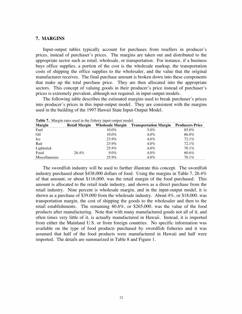
7. MARGINS Input-output tables typically account for purchases from resellers in producer’s prices, instead of purchaser’s prices. The margins are taken out and distributed to the appropriate sector such as retail, wholesale, or transportation. For instance, if a business buys office supplies, a portion of the cost is the wholesale markup, the transportation costs of shipping the office supplies to the wholesaler, and the value that the original manufacturer receives. The final purchase amount is broken down into these components that make up the total purchase price. They are then allocated into the appropriate sectors. This concept of valuing goods in their producer’s price instead of purchaser’s prices is extremely prevalent, although not required, in input-output models. The following table describes the estimated margins used to break purchaser’s prices into producer’s prices in this input-output model. They are consistent with the margins used in the building of the 1997 Hawaii State Input-Output Model. Table 7. Margin rates used in the fishery input-output model. Margin Retail Margin Wholesale Margin Transportation Margin Producers Price Fuel 10.0% 5.0% 85.0% Oil 10.0% 4.0% 86.0% Ice 23.9% 4.0% 72.1% Bait 23.9% 4.0% 72.1% Lightstick 25.9% 4.0% 70.1% Food 26.4% 9.0% 4.0% 60.6% Miscellaneous 25.9% 4.0% 70.1% The swordfish industry will be used to further illustrate this concept. The swordfish industry purchased about $438,000 dollars of food. Using the margins in Table 7, 26.4% of that amount, or about $116,000, was the retail margin of the food purchased. This amount is allocated to the retail trade industry, and shown as a direct purchase from the retail industry. Nine percent is wholesale margin, and in the input-output model, it is shown as a purchase of $39,000 from the wholesale industry. About 4%, or $18,000, was transportation margin, the cost of shipping the goods to the wholesaler and then to the retail establishments. The remaining 60.6%, or $265,000, was the value of the food products after manufacturing. Note that with many manufactured goods not all of it, and often times very little of it, is actually manufactured in Hawaii. Instead, it is imported from either the Mainland U.S. or from foreign countries. No specific information was available on the type of food products purchased by swordfish fisheries and it was assumed that half of the food products were manufactured in Hawaii and half were imported. The details are summarized in Table 8 and Figure 1.

13

Table 8. Breakdown of food product purchases of the swordfish fishery industry into producer’s prices. Industry Agriculture - Mining and construction Food processing $132,711 Other manufacturing - Transportation $17,520 Information - Utilities - Wholesale trade $39,419 Retail trade $115,630 Finance and insurance - Real estate and rentals - Professional services - Business services - Educational services - Health services - Arts and entertainment - Hotels - Eating and drinking - Other services - Government - Imports $132,711 Total $437,992

Figure 1. Percentage breakdown of food product purchases of the swordfish fishery industry into producers prices.

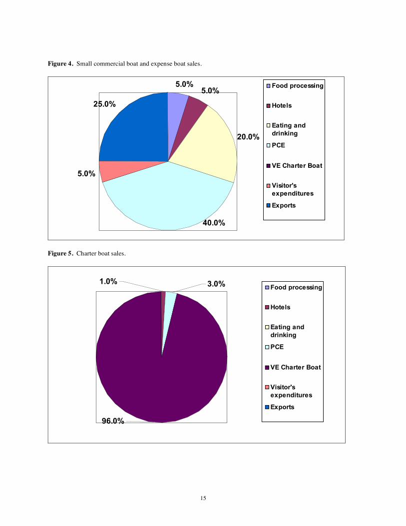
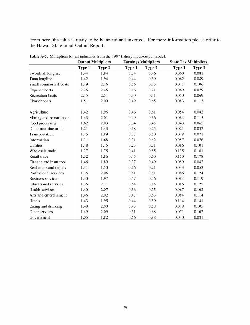
Producer’s prices are used for all types of goods that are purchased through resellers (retailers, wholesalers, etc). The margin rates used are average margins that were originally used to build the U.S. Input-Output Model, and modified to account for the differences between retail and wholesale operations in Hawaii for the Hawaii Input-Output Model. 8. FISHERY SALES Different fishery sectors sell to different types of industries and consumers. Most of the swordfish catch, for instance, gets exported out of the state. Figures 2 through 5 show the differences between the sales of the fishery sectors.

14

Figure 2. Swordfish sales.

5.5%

90.0%

0.5%

1.0%

2.0%1.0%

Food processing

Hotels

Eating and

drinking

PCE

VE Charter Boat

Visitor's

expenditures

Exports

Figure 3. Tuna sales.

15

Figure 4. Small commercial boat and expense boat sales.

5.0%5.0%

20.0%

5.0%

25.0%

40.0%

Food processing

Hotels

Eating and

drinking

PCE

VE Charter Boat

Visitor's

expenditures

Exports

Figure 5. Charter boat sales.

1.0% 3.0%

96.0%

Food processing

Hotels

Eating and

drinking

PCE

VE Charter Boat

Visitor's

expenditures

Exports

16

The direct requirements table shows the input-output table in ratio form where instead of seeing the purchases as the actual value it shows the purchases of each industry as a percent of total output. The direct requirements table is produced as part of the process to generate multipliers. Table 9. Direct requirements table (fishery sectors only).

Swordfish longline

Tuna longline

Small commercial

boats Expense

boats Recreation

boats Charter

boats Swordfish longline 0 0 0 0 0 0 Tuna longline 0 0 0 0 0 0 Small commercial boats 0 0 0 0 0 0 Expense boats 0 0 0 0 0 0 Recreation boats 0 0 0 0 0 0 Charter boats 0 0 0 0 0 0 Agriculture 0 0 0 0 0 0 Mining and construction 0 0 0 0 0 0 Food processing 0.00950 0.02578 0.03557 0.08451 0.07002 0.01577 Other manufacturing 0.07761 0.04993 0.10611 0.31147 0.28694 0.10391 Transportation 0.01473 0.00939 0.01231 0.03158 0.03017 0.08328 Information 0 0 0 0 0 0.01231 Utilities 0 0 0 0 0 0 Wholesale trade 0.15939 0.12163 0.13164 0.20212 0.10348 0.01805 Retail trade 0.00510 0.00769 0.00762 0.02333 0.02258 0.00222 Finance and insurance 0.01186 0.01362 0.01071 0.04808 0.05633 0.06031 Real estate and rentals 0 0 0 0 0 0 Professional services 0 0 0 0 0 0 Business services 0.00695 0.00591 0.00373 0.01707 0.01259 0.02786 Educational services 0 0 0 0 0 0 Health services 0 0 0 0 0 0 Arts and entertainment 0 0 0 0 0 0.01021 Hotels 0 0 0 0 0 0.03830 Eating and drinking 0 0 0 0 0 0.00262 Other services 0.04648 0.07084 0.06052 0.20782 0.24334 0 Government 0.00290 0.00696 0.00264 0.01266 0.01799 0 Earnings 0.21838 0.31598 0.43020 -0.17570 0.00000 0.36003 9. MULTIPLIERS The major feature of an input-output model is the ability to generate economic multipliers. Many different types of multipliers can be generated such as output, or final demand multipliers, income multipliers, and job multipliers. All of these multipliers were generated for the 1997 Hawaii Fisheries Input-Output Model. Multipliers give economists and analysts the ability to estimate the economic impacts of changes in the economy. It needs to be understood that input-output multipliers are average

17

multipliers, not marginal ones. They are computed using what an entire industry consumes and sells averaged over all establishments in that industry over an entire year. Thus, if on the average an industry spends 5 cents on insurance the model estimates for the next dollar an establishment within that industry earns, it will spend 5 cents of that dollar on insurance. The model does not take into account marginal sales and expenditures. Input-output multipliers are often used to estimate the marginal effect of small changes in an industry simply because they are the only tools available to do the analysis. Care needs to be taken when using input-output multipliers to make sure that the tools provided by an input-output table are being used appropriately. The multipliers generated with the 1997 Hawaii Fishery Input-Output Model are not exactly comparable to those from the 1992 model. This is caused by two changes in the way the State Input-Output model was built: different estimates of Gross State Product used to build the model and different methods for calculating multipliers. The multipliers were generated using the RIMS II methodology from the U.S. BEA. This change in methodology results in higher type 1 multipliers and lower type 2 multipliers in 1997 compared to 1992. Earnings multipliers are also lower in 1997 because of the methodology change. In brief, the RIMS II methodology adjusts for taxes and savings when computing multipliers more realistically than what was used in the 1992 model. The 1997 Hawaii State Input-Output Report (DBEDT, 2003) contains a detailed section explaining the changes between 1992 and 1997. 9.1 Type I Multipliers In order to understand economic multipliers, it is necessary to understand the types of impacts that are estimated by economic multipliers. There are three types of effects that make up multipliers—the direct effect, indirect effect, and induced effect. The direct effect is simply the initial dollars spent that are being measured. The indirect effect is the effect of industries purchasing extra goods and services needed to produce the extra goods and services demanded by the direct effect, without accounting for the increases due to changes in household income and expenditures. For example, what would occur if the demand for exported swordfish increased by $1 million? In order to produce the extra $1 million in swordfish, the fisheries industry would need to by bait, food, ice, gasoline, boats, insurance, etc. When the fishery buys these goods the producers of those goods also need to buy more goods in order to produce their wares to sell. In turn the suppliers of the manufacturers would also need more goods, and then their suppliers would need to do the same, and so on. This chain of events is called the multiplier effect. 9.2 Type II Multipliers Type II multipliers include effects that are listed under Type I multipliers (direct and indirect effects) and also include induced effects caused by changes in household income and expenditures. For example, to fill demand for an additional $1 million of swordfish, fisheries companies would need supplies such as bait, food, ice, gasoline, etc. However, they also need labor in order to catch and process the fish. The additional wages and salaries are spent on goods and services that in turn require producers of those goods and services need to purchase goods,

18

services, and labor in order to meet the additional demand. Once again, the multiplier effect comes into play and sets off a sequence of events. In Table 10 we compare some key multipliers between 1992 and 1997. Note that the multipliers are based on the methodologies used in the 1992 and 1997 Hawaii State Input-Output reports and those methodologies differ from each other. The change in methodology typically results in higher type 1 multipliers and lower type 2 multipliers in 1997 compared to 1992. Also, earnings multipliers are lower in 1997 as well due to the methodology change. The Hawaii State Input-Output Report contains a detailed section explaining the changes between 1992 and 1997. Table 10. Key Multipliers for Fishery Sectors, 1997 and 1992. Output Multipliers Earnings Multipliers Total Jobs Multipliers Type 1 Type 2 Type 1 Type 2 Type 1 Type 2 1997 Swordfish longline 1.44 1.84 0.34 0.46 14.64 19.34 Tuna longline 1.42 1.94 0.44 0.59 20.12 26.15 Small commercial boats 1.49 2.16 0.56 0.75 49.69 57.39 Expense boats 2.26 2.45 0.16 0.21 270.62 272.77 Recreation boats 2.15 2.51 0.30 0.41 13.63 17.80 Charter boats 1.51 2.09 0.49 0.65 22.11 28.81 1992 Longline fishery 1.47 2.32 0.60 0.91 19.07 30.87 Other commercial fishery 1.61 2.38 0.54 0.83 30.89 41.61 Charter fishery 1.74 2.59 0.60 0.92 33.24 45.14 Recreational/expense fishery

1.98 2.33 0.25 0.37 8.52 13.39

10. CONCLUSIONS The 1997 Hawaii Fishery Input-Output Model is a step forward in understanding and analyzing the economics of the fisheries industry in Hawaii. The model expands the fishery industry into more detail than before, captures the visitor industry impact of charter boat fishing, and incorporates the updated and improved methodologies of the 1997 Hawaii State Input-Output Model. Although this model is an improvement over the previous model it can still be refined further. In order to do that, however, more and better data are needed. Specifically, better data is needed on how employment within fishery industries works—in terms of self-employment versus wage and salary employment, how crew members get paid, how their income and employment are reported to the government, and how it is translated into the macroeconomic data reported by BEA and other sources. Businesses operating in the fisheries industries seem to have operations that are somewhat different from most other types of businesses and the data collected on fisheries might be subject to misinterpretation because of this.

19

11. REFERENCES Bureau of Economic Analysis, U.S. Department of Commerce, SA-05 Personal Income by Major

Source and Earnings by Industry 1958-2000, Electronic File, September 2001. Bureau of Economic Analysis, U.S. Department of Commerce, SA-07 Wage and Salary

Disbursements by Industry 1958-2000, HTML File, September 2001. Bureau of Economic Analysis, U.S. Department of Commerce, SA-25 Total Full-time and Part-

time Employment by Industry 1958-2000, Electronic File, September 2001. Bureau of Economic Analysis, U.S. Department of Commerce, SA-27 Wage and Salary

Employment by Industry 1958-2000, Electronic File, September 2001. Bureau of Economic Analysis, U.S. Department of Commerce, Input-Output Accounts of the

United States, 1992, September 1998. Department of Business, Economic Development and Tourism (2003). The Hawaii input-output

study: 1997 benchmark report. Research and Economic Analysis Division, Hawaii DBEDT. Hamilton, M.S. and S.F. Huffman (1997). Cost-earnings study of Hawaii’s small boat fishery,

1995-1996. Pelagic Fisheries Research Program Technical Rep., SOEST 97-06/JIMAR Contribution 97-314, 102 pp., Joint Institute of Marine and Atmospheric Research, University of Hawaii at Manoa.

Hamilton, M.S., R.E. Curtis, and M.D. Travis (1996). Cost-earnings study of Hawaii’s based domestic longline fleet. Pelagic Fisheries Research Program Technical Rep., SOEST 96-03/JIMAR Contribution 96-300, 59 pp., Joint Institute of Marine and Atmospheric Research, University of Hawaii at Manoa.

O’Malley, J.M. and E. W. Glazier (2001). Motivations, satisfaction and expenditures of recreational and pelagic charter fishing patrons in Hawaii. Pelagic Fisheries Research Program Technical Rep., SOEST 01-03/JIMAR Contribution 01-339, 46 pp., Joint Institute for Marine and Atmospheric Science, University of Hawaii at Manoa.

20

APPENDIX This section gives a brief yet technical description of the steps taken to build the 1997 Fishery Input-Output Model. Data Sources There were several sources of data used to build this model. First, and most importantly, the 1997 Hawaii State Input-Output Model and the 1992 Hawaii Fishery Input-Output Model are the primary sources of information. The data used to build the production functions for the longline commercial fishing came from a 1993 survey of longline fisheries (Hamilton et al., 1996). The data for the production functions of the small commercial boat, and the expense/recreational boats came from a cost-earnings survey done in 1995-96 (Hamilton and Huffman, 1997). The charter boat production function was simply borrowed from the 1992 model. Data from a charter boat patron survey done in 2000 (O’Malley et al., 2001) was used in part to build a charter boat visitor consumption function. The 1997 Hawaii State Input-Output Model is the basis for building the fishery model. The fishery model was designed to be consistent with the methodology and definitions used in the 1997 State Input-Output Model. These methodology and definitions are different than those used in the 1992 input-output model. Methodology This section describes the methods used to create the production functions for each fishery industry. The methods differ depending on the sources of information available. This section gives an overview of the methods used as well as a detailed, step-by-step approach to building the production function for the swordfish longline fishery. Commercial Longline The data for the tuna and swordfish sectors came from the 1993 cost-earnings survey of longline fisheries done by Hamilton et al. (1996). There was a similar survey done in 2000 and the results of the two surveys looked quite similar, however, the 1993 data was used because it looked cleaner and was easier to work with. The process of building the production function involves several steps. First, an initial production function was made by allocating the average costs of goods and services purchased into the appropriate industries in the model. The value added portion of the model which was made up of compensation of employees, proprietor’s income, taxes, and other capital costs (mainly depreciation and corporate profits) was estimated from the information in the survey. The value added section was adjusted based on the total valued added for commercial fishing from the 1997 Gross State Product from the 2004 U.S. Bureau of Economic Analysis (www.bea.gov/bea/regional/gsp.htm). The GSP for all commercial fishing sectors needed to add up to the total for all commercial fishing so some balancing and adjusting was done to make sure all the sectors added up to the control totals for GSP.

21

Once the initial production functions were built for all of the commercial fishing sectors (except charter boats), the value added sections were balanced so that they added up to the total from the GSP accounts. Each of the four sections of the GSP were adjusted and balanced separately, and were then balanced proportionately based on the amounts of each GSP item in the commercial fishing sectors. After the value added was balanced, the rest of the production function was adjusted and balanced so that the total production function added up to 100%. This was also done proportionately within each commercial fishing sector. To be consistent with the methodology for building input-output tables, any purchases of goods needed to be turned into producer’s prices. The transportation, wholesale, and retail margins were reallocated into their respective sectors. It should be noted that the building of the commercial boat sectors deviated slightly from the exact methodology used to build input-output tables. This deviation occurred in the wholesale sector. Many commercial fisheries sell their fish at wholesale auction, and the auction takes roughly 10% of the sale price as their fee. The 10% is reported as commercial fishery revenue, and also as a cost to the fisheries. Normally in input-output, the margin would be taken out of the fishery revenue and reallocated to the wholesale sector. Thus, the fishery revenue would be 10% lower, and their wholesale expense would be lower by the same dollar amount. Thus, in order to get the full impact of the fishery industry you would need to calculate the impact using the commercial fishing sector as well as the wholesale sector because the fishery sector by itself would not contain all of the impact of the industry. For this model auction fees are kept as fishery revenue and the 10% fees are expenses paid to the wholesale sector. Building the model this way inflates the overall multipliers, although probably by a small but measurable amount. Small Commercial Boats The small commercial boat production functions were built primarily with data from the small boat cost-earnings survey done in 1995-96. This was done using the same general methods as the longline fisheries—first build a preliminary production function, transfer to producer prices, balance the value added, and then balance the rest of the production function. Expense/Recreational Boats There were fairly significant changes to the expense and recreational boats sectors for this model. First, they were split into separate sectors. In the previous model, there were no jobs or value added associated with either. That has changed this time. Because the expense boats actually sell part of their catch, they are considered to be in business. They file self-employed tax returns, and thus are considered to be self-employed even if they just sell their catch to cover their expenses and even if there is a very small amount of money involved. In fact, they make up the majority of the self-employed jobs in the commercial fishing sector. They also have a value added component to them. If they are in business they pay taxes, depreciate their assets, and have profits or losses. Expense fishermen usually experience losses, which show up as negative proprietor’s income in the table. This is acceptable and expected because they are not trying to earn a profit. The data from the small boat survey shows that in most instances their expenses exceed their income.

22

One troubling part of putting this data into the model this year was that their expenses are significantly larger than their income. Initially the difference between expense and income was computed as negative proprietor’s income but it was so large that it produced unreasonable results for all of the commercial fishing sectors when the data were balanced to BEA control totals for proprietor’s income. Further examination of the data revealed that expense boats sell only 59% of their catch, keeping the difference for themselves. Therefore, because 41% of the cost does not go to towards catching fish that are ultimately sold, that 41% was taken out of the expense sector. This cost was then added to the recreational sector because that 41% can better be defined as recreational fishing. Ultimately, it is debatable whether this is a correct assumption or not. In order to confirm the accuracy of this assumption, we would have to know how expense fisherman filled out their tax returns. If all fishing expenses are being written off as business expenses and the fishermen are taking a rather large loss, then our conclusion is not correct. However, it seems more reasonable to assume that the expense fishermen were only able to write off part of their expenses as opposed to all of them. One rather important point of note: although nationally accepted definitions of output, value added, etc., for commercial fishing are used, the amount of fish kept by the fishermen is not recorded as output. This is in contrast to the agricultural sector where estimates of farm products grown and consumed on the farm are imputed and added to actual sales to get total output. The methodology of the U.S. input-output model specifically states that catch kept by fishermen is not added in for commercial fishing. Charter Boats The charter boat sector was estimated based on the 1992 charter boat sector and the data on charter boats from the 1997 U.S. Economic Census (www.census.gov/epcd/ec97/hi/ HI000_48.HTM). In 1992, the charter boat output was $16.5 million and in 1997 it was $14.2 million. In 1997, there was specific data in the U.S. Economic Census related to charter boats that was not available in previous years. One major difference in the charter boat sector compared to 1992 is that the number of jobs is much lower. There are two sources of information on wage and salary jobs—one is the U.S. Economic Census, and the other is BEA. The number of jobs from BEA was 175, much lower than in 1992 when it was 325. According to the U.S. Economic Census the number of jobs was 142, although there is usually some undercounting in this data. The U.S. Economic Census output was used and adjusted for undercounting using the same method of adjustment used to create the 1997 input-output table. In 1992, charter boat fishing was lumped in with miscellaneous amusement services. Because there is no way to extract just the charter boat jobs and income, the 1997 data is probably much more accurate than the 1992 data. Another adjustment made to the 1997 output that was not done to the 1992 data was that tips paid to crew were added to the output. The amount of tips paid to the crew was around $1.2 million. Because there was no additional information on charter boat expenses, the 1992 production function was used and adjusted to balance with the value added portion of the charter boat sector. In the 1997 State Input-Output Model, which was built using the newer NAICS industry classification system, charter boats are no longer listed in miscellaneous amusement services but in an industry called sightseeing transportation. Because no information on certain parts of value

23

added for charter boats was available, the ratio of other capital costs to output for sightseeing was used to calculate other capital costs for charter boats. In 1996, there were 188 commercial charter boat licenses issued by the state of Hawaii, therefore, it was assumed that there were 188 active charter boats running. However, the 1997 Economic Census only lists 42 establishments with employees in the charter boat industry. Most of these had only one boat, but there probably were a few that operated more than one boat. The number of non-employer establishments in the entire sightseeing transportation sector in 1997 (non-employer charter boat data was suppressed) was only 67. This says that although there were 188 charter boats with licenses to operate, not all of them were actually operating commercially. A casual search on the Internet for charter boats yielded approximately 100-120 active charter boats operating in 2003. Visitor Expenditure, Charter Boats A charter boat patron survey was completed in 2000 and the data was used to create a visitor expenditure vector for visitors who went on fishing charters. The charter patron survey does not include a comprehensive set of visitor expenditures; it only includes expenditures for the one day that they went on a charter. This data was combined with average U.S. visitor expenditures for non-fishing days. Sales of Commercial Fishing Industries There is little data available on where the sales of fish go and this applies to each of the fishery sectors. The only hard data available for commercial sales was for exports. The total exports for commercial fishing were different from the 1997 Hawaii State Input-Output model, and because exports were part of GSP, that number changed. Because GSP is a fixed number that is not allowed to change another part of GSP, namely imports, was adjusted to keep GSP fixed. This is a procedure that was also used in building the Hawaii State Input-Output Model. Instead of adjusting the PCE for commercial fishing from the State Input-Output Model we simply allocated it into the different fishery sectors. Charter boat PCE expenses and visitor expenses were estimated from data in the charter patron survey. Transactions Table Once the production functions were created a complete, balanced transactions table was created. The methods of doing this are described in detail in the 1997 Hawaii State Input-Output Report. It should also be noted that with regard to balancing the data, the fishery sectors were not allowed to adjust in the balancing procedure. The numbers were fixed so the non-fishery sectors were adjusted so that the table balanced. From there, the inverting of the matrix and creation of the multipliers follows the procedures detailed in the Hawaii State Input–Output Report.

24

Recommendations for the Future In order to build more accurate fishery input-output models in the future, more and better information is needed. For example, if cost-earnings studies are performed in the future they need to be more comprehensive with regard to the types of expenses incurred by the fisheries. Asking questions that cover only five categories is not comprehensive enough. Businesses have many expenses that are not “top of mind” expenses and survey respondents often forget about them. The survey needs to probe deeper and ask specific questions about things like legal services, automotive expenses, travel and other transportation expenses, and communication expenses (both on and off land). Any information that can be gained from wholesale auctions would be very useful. Specifically, information on who buys the fish at auction (i.e., restaurants, grocery stores, hotels, food processors, etc.) would be very valuable. Also, the existing information about jobs and income and how the crews are paid is not in a useful format because it is unclear exactly how it fits into the macroeconomic data from other sources used to build these models. Asking questions like, “Did you file a self-employed tax return?” “Did your crew file self-employed tax returns?” “Do you report for unemployment insurance purposes any of your crew as employees?” would give much better information on how jobs and income from the survey fit into the macroeconomic data. With regard to the charter patron survey, although the survey is actually quite good there are some subtle areas that can cause problems. One such area is in the expenses of the charter itself. The question does not specify if charter operators are to base their answers on each charter group or each individual in the group. Examination of the data reveals that respondents did both and that compromises the integrity of the results. It’s such an easy thing to overlook and can have a significant effect on the results. Detailed Methodology on Building Longline Production Functions This section describes in detail the methods used to build the longline production functions. The methods used to build the other production functions were built in a similar fashion. This section is added to give NMFS and JIMAR a roadmap so that in the future, they would have the option of updating the model themselves. The cost-earnings data was used as a starting point for building the production functions. The data are in Table A-1. These are the raw data used to build the production functions. Because the data was not in a usable format, however, they needed to be transformed into producer’s prices. This means that margins for wholesale, retail, and transportation needed to be computed. The margins were taken from the 1997 Hawaii State Input-Output Model Appendix C. (see Table A-2)

25

Table A-1. Cost and earnings information for swordfish and tuna. Cost and Earnings Information Swordfish Per Year Tuna Per Year Revenue $632,596 $355,473 Variable costs Fuel $66,551 $25,504 Oil $3,092 $1,168 Ice $3,687 $10,209 Bait $68,792 $31,447 Lightsticks $56,049 $0 Food $14,082 $12,653 Misc. gear $39,515 $14,540 Captain wages $46,642 $39,531 Other crew wages $92,257 $73,385 Excise taxes $3,163 $1,777 Sales fees $65,873 $35,284 Total variable costs $494,704 $245,498 Net operating return $137,892 $109,975 Fixed costs Maintenance $26,419 $21,993 Drydock $7,459 $8,766 Mooring $2,117 $3,021 Insurance $34,585 $23,660 Accounting $5,067 $2,565 Loan payments $22,041 $17,916 Miscellaneous $11,146 $1,379 Depreciation charge $17,983 $10,189 Total fixed costs $126,817 $89,489 Total costs $621,521 $334,987 Net return $46,075 $20,486 Add back non-cash $17,983 $10,189 Depreciation charge Cash return $64,058 $30,676

26

Table A-2. Margins used to compute producer’s prices.

Margin Margin Value Swordfish Tuna Fuel wholesale margin 0.1 $6,655.10 $2,550.40 trans margin 0.05 $3,327.55 $1,275.20 producers price 0.85 $56,568.35 $21,678.40 Oil wholesale margin 0.1 $309.20 $116.80 trans margin 0.04 $123.68 $46.72 producers price 0.86 $2,659.12 $1,004.48 Ice wholesale margin 0.239 $881.19 $2,439.95 trans margin 0.04 $147.48 $408.36 producers price 0.721 $2,658.33 $7,360.69 Bait wholesale margin 0.239 $16,441.29 $7,515.83 trans margin 0.04 $2,751.68 $1,257.88 producers price 0.721 $49,599.03 $22,673.29 Lightstick wholesale margin 0.259 $14,516.69 $0.00 trans margin 0.04 $2,241.96 $0.00 producers price 0.701 $39,290.35 $0.00 Food retail 0.264 $3,717.65 $3,340.39 wholesale margin 0.09 $1,267.38 $1,138.77 trans margin 0.04 $563.28 $506.12 producers price 0.606 $8,533.69 $7,667.72 Misc. gear wholesale margin 0.259 $10,234.39 $3,765.86 trans margin 0.04 $1,580.60 $581.60 producers price 0.701 $27,700.02 $10,192.54 Once producer’s prices were calculated, the margins were assigned to their appropriate industry: wholesale margins went to the wholesale industry, and so forth. The producer’s value can be assigned to one of two areas. It can be assigned to the Hawaii based industry that produces it or it can be considered an import. Most of the producer’s values were assigned as imports because Hawaii produces limited manufactured goods, with a few exceptions. Fuel oil was assigned as a domestically produced good because there are oil refineries in Hawaii. All of the ice and half of the food consumed on longline boats was assumed to be produced in Hawaii, and assigned to the food processing industry. The rest of the food was allocated to imports. The fixed costs were assigned to the industry with the most logical fit. Maintenance and dry-dock costs were assigned to the other services sector because boat building and maintenance is a sub-industry of that sector in NAICS.

27

There are several fixed costs that were classified as other capital costs, which is part of value added. They are profit, depreciation, and net interest paid. The definitions of profit, depreciation, and net interest paid are different in value added from how they are defined in the cost-earnings study, although they can be considered to be similar. The fixed costs that fall under value added were assigned as other capital costs, and then the other capital costs were balanced so that all of the commercial fishing sectors added up to the commercial fishing other capital costs as published by BEA. The unbalanced per boat production function is in Table A-3.

Table A-3. Unbalanced production function (per boat). Industry Swordfish Tuna

Agriculture Mining and construction Food processing $6,925 $11,195 Other manufacturing $56,568 $21,678 Transportation $10,736 $4,076 Information Utilities Wholesale trade $116,178 $52,812 Retail trade $3,718 $3,340 Finance and insurance $34,585 $23,660 Real estate and rentals Professional services Business services $5,067 $2,565 Educational services Health services Arts and entertainment Hotels Eating and drinking Other services $33,878 $30,759 Government $2,117 $3,021 Compensation of employees $101,996 $83,562 Tax $3,163 $1,777 Imports $123,515 $37,704 Other capital costs $97,245 $49,970 Proprietor income $36,903 $29,354 Total $632,595 $355,473 For each of the value added sections (compensation of employees, proprietors’ income, indirect business taxes, and other capital costs), a preliminary amount was calculated for each commercial fishing sector. Then, for each sector, the amount for each commercial fishing sector was adjusted proportionately so that all commercial fishing sectors added up to the control total from BEA. In order for the production function to add up to 100% of output, the intermediate inputs needed to be adjusted and balanced because the other capital costs changed (remember, our unbalanced production functions added up to 100%, but now do not because the value added

28

components changed slightly). These were simply adjusted proportionately. For example, if the sum of the intermediate inputs was 50% of total output before value added was balanced, and is supposed to be 51.4% of output after value added was balanced, then each component of the intermediate demand vector is multiplied by (0.514/0.500) so that the production function again adds up to 100%. It should be noted that the compensation of employees and proprietors’ income was somewhat difficult to produce. There are two sources of information that do not fit together very well. The cost-earnings data gives three possible labor income categories: captain’s wages, other crew wages, and net profit (proprietors income). BEA gives wage and salary income and jobs and proprietor’s income and jobs. It was assumed that captains and crew can be either wage and salary employees (the employer pays unemployment insurance on the employees) or they can be proprietors (where they are responsible for paying their own Social Security taxes, etc.), depending on their arrangement with their employer. Looking at the BEA jobs data, it appears that both types occur in the sector. According to the data there are 340 wage and salary jobs in the commercial fishing sector. When examining the number of commercial fishing boats and the average crew per boat, however, there are a total of over 600 jobs listed in the longline sector alone. Therefore it seems logical to assume that there must be close to 300 captains or crew that are self-employed, at least for tax purposes. Ultimately, there is a question of whether one source of data is better than the other when breaking down wage and salary versus proprietors’ jobs. Ultimately, the two combined are much more reliable than either of the two separately. The same can be said for wage and salary income and proprietors’ income. The total jobs were computed based on the total income of employees, wage and salaried and proprietors, divided by average crew wages. They were then allocated and balanced into wage and salaried vs. proprietors jobs based on BEA control totals for those jobs (see Table A-4).

Table A-4. Job computations for longline fishing. Swordfish Tuna W&S income 4,148,256 7,302,649 Proprietors income 1,454,288 2,485,698 Average number of crew (incl. captain) 5.40 4.69 Average income/crew (incl. captain) 25,699 24,089 Total jobs (total income/average income) 218 406 W&S jobs 116 215 Proprietors jobs 102 191 At this point the production functions are more or less finished. They may need revision after inverting the table and checking the multipliers. It is also good to check job/income ratios and income/output ratios before doing that, just to see if there are any ratios that look too high or low.

29

From here, the table is ready to be balanced and inverted. For more information please refer to the Hawaii State Input-Output Report. Table A-5. Multipliers for all industries from the 1997 fishery input-output model.

Output Multipliers Earnings Multipliers State Tax Multipliers Type 1 Type 2 Type 1 Type 2 Type 1 Type 2

Swordfish longline 1.44 1.84 0.34 0.46 0.060 0.081 Tuna longline 1.42 1.94 0.44 0.59 0.062 0.089 Small commercial boats 1.49 2.16 0.56 0.75 0.071 0.106 Expense boats 2.26 2.45 0.16 0.21 0.069 0.079 Recreation boats 2.15 2.51 0.30 0.41 0.050 0.069 Charter boats 1.51 2.09 0.49 0.65 0.083 0.113 Agriculture 1.42 1.96 0.46 0.61 0.054 0.082 Mining and construction 1.43 2.01 0.49 0.66 0.084 0.115 Food processing 1.62 2.03 0.34 0.45 0.043 0.065 Other manufacturing 1.21 1.43 0.18 0.25 0.021 0.032 Transportation 1.45 1.89 0.37 0.50 0.048 0.071 Information 1.31 1.68 0.31 0.42 0.057 0.076 Utilities 1.48 1.75 0.23 0.31 0.086 0.101 Wholesale trade 1.27 1.75 0.41 0.55 0.135 0.161 Retail trade 1.32 1.86 0.45 0.60 0.150 0.178 Finance and insurance 1.46 1.89 0.37 0.49 0.059 0.082 Real estate and rentals 1.31 1.50 0.16 0.21 0.043 0.053 Professional services 1.35 2.06 0.61 0.81 0.086 0.124 Business services 1.30 1.97 0.57 0.76 0.084 0.119 Educational services 1.35 2.11 0.64 0.85 0.086 0.125 Health services 1.40 2.07 0.56 0.75 0.067 0.102 Arts and entertainment 1.46 2.02 0.47 0.63 0.084 0.114 Hotels 1.43 1.95 0.44 0.59 0.114 0.141 Eating and drinking 1.48 2.00 0.43 0.58 0.078 0.105 Other services 1.49 2.09 0.51 0.68 0.071 0.102 Government 1.05 1.82 0.66 0.88 0.040 0.081

30

Table A-5 (cont). Multipliers for all industries from the 1997 fishery input-output model.

W&S job multipliers (jobs/final demand)

W&S job multipliers (jobs/job)

Total job multipliers (jobs/final demand)

Total jobs multipliers (jobs/job)

Type 1 Type 2 Type 1 Type 2 Type 1 Type 2 Type 1 Type 2 Swordfish longline 9.02 12.66 1.83 2.58 14.64 19.34 1.56 2.07 Tuna longline 11.92 16.59 1.57 2.19 20.12 26.15 1.39 1.81 Small commercial boats 5.12 11.09 6.00 12.98 49.69 57.39 1.13 1.30 Expense boats 10.94 12.61 na na 270.62 272.77 1.06 1.07 Recreation boats 10.14 13.37 na na 13.63 17.80 na na Charter boats 16.38 21.56 1.33 1.75 22.11 28.81 1.29 1.69 Agriculture 18.73 23.58 1.27 1.59 31.15 37.41 1.23 1.48 Mining and construction 10.80 16.05 1.52 2.26 14.70 21.47 1.55 2.27 Food processing 13.05 16.66 2.01 2.56 16.50 21.16 2.48 3.18 Other manufacturing 5.12 7.08 1.47 2.03 6.81 9.34 1.46 2.00 Transportation 10.84 14.80 1.54 2.10 12.42 17.52 1.61 2.28 Information 7.97 11.31 1.39 1.98 9.67 13.98 1.46 2.11 Utilities 4.93 7.40 2.18 3.27 5.85 9.05 2.58 3.99 Wholesale trade 12.19 16.55 1.20 1.63 14.77 20.39 1.24 1.71 Retail trade 18.95 23.76 1.14 1.43 24.04 30.25 1.15 1.45 Finance and insurance 8.99 12.90 1.50 2.15 12.95 17.99 1.50 2.08 Real estate and rentals 4.00 5.70 2.57 3.66 6.85 9.04 2.03 2.68 Professional services 10.83 17.27 1.29 2.05 19.90 28.21 1.22 1.73 Business services 22.84 28.85 1.15 1.45 28.87 36.63 1.16 1.47 Educational services 24.85 31.65 1.09 1.38 32.91 41.69 1.09 1.39 Health services 15.02 21.00 1.22 1.71 17.41 25.13 1.28 1.85 Arts and entertainment 19.20 24.22 1.22 1.54 29.06 35.55 1.21 1.47 Hotels 15.22 19.89 1.30 1.70 16.70 22.73 1.40 1.91 Eating and drinking 25.21 29.81 1.17 1.38 27.26 33.19 1.23 1.49 Other services 18.92 24.32 1.21 1.55 27.28 34.25 1.20 1.51 Government 19.15 26.14 1.02 1.39 19.28 28.30 1.03 1.51