© 1991 John Wiley & Sons, Inc. 14 - opt.zju.edu.cnopt.zju.edu.cn/zjuopt2/upload/resources/chapter14 Lasers.pdf · Bahaa E. A. Saleh, Malvin Carl Teich Copyright © 1991 John Wiley

CHAPTER

14 LASERS

14.1 THEORY OF LASER OSCILLATION A. Optical Amplification and Feedback 6. Conditions for Laser Oscillation

14.2 CHARACTERISTICS OF THE LASER OUTPUT A. Power B. Spectral Distribution C. Spatial Distribution and Polarization D. Mode Selection E. Characteristics of Common Lasers

14.3 PULSED LASERS A. Methods of Pulsing Lasers

*B. Analysis of Transient Effects *C. Q-Switching

D. Mode Locking

In 1958 Schawlow, together with Charles Townes, showed how to extend the principle of the maser to the optical region. He shared the 1981 Nobel Prize with Nicolaas Bloembergen. Maiman demonstrated the first successful operation of the ruby laser in 1960.

494

Fundamentals of PhotonicsBahaa E. A. Saleh, Malvin Carl TeichCopyright © 1991 John Wiley & Sons, Inc.ISBNs: 0-471-83965-5 (Hardback); 0-471-2-1374-8 (Electronic)

The laser is an optical oscillator. It comprises a resonant optical amplifier whose output is fed back into its input with matching phase (Fig. 14.0-l). In the absence of such an input there is no output, so that the fed-back signal is also zero. However, this is an unstable situation. The presence at the input of even a small amount of noise (containing frequency components lying within the amplifier bandwidth) is unavoidable and may initiate the oscillation process. The input is amplified and the output is fed back to the input, where it undergoes further amplification. The process continues indefinitely until a large output is produced. Saturation of the amplifier gain limits further growth of the signal, and the system reaches a steady state in which an output signal is created at the frequency of the resonant amplifier.

Two conditions must be satisfied for oscillation to occur:

. The amplifier gain must be greater than the loss in the feedback system so that net gain is incurred in a round trip through the feedback loop.

. The total phase shift in a single round trip must be a multiple of 2n so that the fedback input phase matches the phase of the original input.

If these conditions are satisfied, the system becomes unstable and oscillation begins. As the oscillation power grows, however, the amplifier saturates and the gain diminishes below its initial value. A stable condition is reached when the reduced gain is equal to the loss (Fig. 14.0-2). The gain then just compensates the loss so that the cycle of amplification and feedback is repeated without change and steady-state oscillation ensues.

Because the gain and phase shift are functions of frequency, the two oscillation conditions are satisfied only at one (or several) frequencies, called the resonance frequencies of the oscillator. The useful output is extracted by coupling a portion of the power out of the oscillator. In summary, an oscillator comprises:

. An amplifier with a gain-saturation mechanism

. A feedback system

. A frequency-selection mechanism n An output coupling scheme

Feedback

Amplifier

Power SUPPlY

Figure 14.0-I An oscillator is an amplifier with positive feedback.

495

496 LASERS

t Gain

Figure 14.0-2 If the initial amplifier gain is greater than the loss, oscillation may initiate. L The amplifier then saturates whereupon its gain 0 t Power decreases. A steady-state condition is reached when the gain just equals the loss.

Steady-state power

Mirror \ Active medium

-d+ mirror -

Figure 14.0-3 A laser consists of an optical amplifier (employing an active medium) placed within an optical resonator. The output is extracted through a partially transmitting mirror.

The laser is an optical oscillator (see Fig. 14.0-3) in which the amplifier is the pumped active medium discussed in Chap. 13. Gain saturation is a basic property of laser amplifiers. Feedback is obtained by placing the active medium in an optical resonator, which reflects the light back and forth between its mirrors, as discussed in Chap. 9. Frequency selection is achieved by the resonant amplifier and by the resonator, which admits only certain modes. Output coupling is accomplished by making one of the resonator mirrors partially transmitting.

Lasers are used in a great variety of scientific and technical applications including communications, computing, image processing, information storage, holography, lithog- raphy, materials processing, geology, metrology, rangefinding, biology, and clinical medicine.

This chapter provides an introduction to the operation of lasers. In Sec. 14.1 the behavior of the laser amplifier and the laser resonator are summarized, and the oscillation conditions of the laser are derived. The characteristics of the laser output (power, spectral distribution, spatial distribution, and polarization) are discussed in Sec. 14.2, and typical parameters for various kinds of lasers are provided. Whereas Sets. 14.1 and 14.2 are concerned with continuous-wave (CW) laser oscillation, Sec. 14.3 is devoted to the operation of pulsed lasers.

14.1 THEORY OF LASER OSCILLATION

We begin this section with a summary of the properties of the two basic components of the laser-the amplifier and the resonator. Although these topics have been discussed in detail in Chaps. 13 and 9, they are reviewed here for convenience.

THEORY OF LASER OSCILLATION 497

A. Optical Amplification and Feedback

Laser Amplification The laser amplifier is a narrowband coherent amplifier of light. Amplification is achieved by stimulated emission from an atomic or molecular system with a transition whose population is inverted (i.e., the upper energy level is more populated than the lower). The amplifier bandwidth is determined by the linewidth of the atomic transition, or by an inhomogeneous broadening mechanism such as the Doppler effect in gas lasers.

The laser amplifier is a distributed-gain device characterized by its gain coefficient (gain per unit length) y(v), which governs the rate at which the photon-flux density C$ (or the optical intensity I = hv4) increases. When the photon-flux density 4 is small, the gain coefficient is

1 (14.1-1)

1 Small-Signal Gain Coefficient

where

N, = equilibrium population density difference (density of atoms in the upper energy state minus that in the lower state); N, increases with increasing pumping rate

a(v) = (n2/87i.t,,)g(v) = transition cross section t SP = spontaneous lifetime

g(v) = transition lineshape h = wavelength in the medium = A,/n, where n = refractive index.

As the photon-flux density increases, the amplifier enters a region of nonlinear operation. It saturates and its gain decreases. The amplification process then depletes the initial population difference N,, reducing it to N = NO/[1 + +/4,(v)] for a homogeneously broadened medium, where

C#J$V) = [r&v)]-’ = saturation photon-flux density 7, = saturation time constant, which depends on the decay times of the energy

levels involved; in an ideal four-level pumping scheme, rS = tsp, whereas in an ideal three-level pumping scheme, rS = 2t,,.

The gain coefficient of the saturated amplifier is therefore reduced to y(v) = Nub), so that for homogeneous broadening

The laser amplification process also introduces a phase shift. When the lineshape is Lorentzian with linewidth Av, g(v) = (Av/27r)/[(v - vO>2 + (Av/~)~], the amplifier

498 LASERS

Gain coefficient

A4

Figure 14.1-l Spectral dependence of the amplifier with Lorentzian lineshape function.

gain and phase-shift coefficients for an optical

phase shift per unit length is

This phase shift is in addition to that introduced by the medium hosting the laser atoms. The gain and phase-shift coefficients for an amplifier with Lorentzian lineshape function are illustrated in Fig. 14.1-1.

Feedback and Loss: The Optical Resonator Optical feedback is achieved by placing the active medium in an optical resonator. A Fabry-Perot resonator, comprising two mirrors separated by a distance d, contains the medium (refractive index n) in which the active atoms of the amplifier reside. Travel through the medium introduces a phase shift per unit length equal to the wavenumber

(14.1-4) Phase-Shift Coefficient

The resonator also contributes to losses in the system. Absorption and scattering of light in the medium introduces a distributed loss characterized by the attenuation coefficient (Y, (loss per unit length). In traveling a round trip through a resonator of length d, the photon-flux density is reduced by the factor 9,9, exp( -2a,d), where S1 and S2 are the reflectances of the two mirrors. The overall loss in one round trip can therefore be described by a total effective distributed loss coefficient cy,., where

exp( - 2a,d) = SIB2 exp( - 2a,d),


so that

(14.1-5)

Loss Coefficient

where cy,, and CY,,,~ represent the contributions of mirrors 1 and 2, respectively. The contribution from both mirrors is

1 awl = ffml + a,2

=Lln- 2d c%‘@‘2’

Since cy, represents the total loss of energy (or number of photons) per unit length, (Y,C represents the loss of photons per second. Thus

1 rP = (yc

r

(14.1-6)

represents the photon lifetime. The resonator sustains only frequencies that correspond to a round-trip phase shift

that is a multiple of 2~. For a resonator devoid of active atoms (i.e., a “cold” resonator), the round-trip phase shift is simply k2d = 4rud/c = q27r, corresponding to modes of frequencies

Vq = qvF, q = 1,2, . . . , (14.1-7)

where VF = c/2d is the resonator mode spacing and c = c,/n is the speed of light in the medium (Fig. 14.1-2). The (full width at half maximum) spectral width of these resonator modes is

VF 6u = -

<F (14.1-8)

where St is the finesse of the resonator (see Sec. 9.1A). When the resonator losses are

-I C ‘F = 2d I---

A Resonator

6

VIQ - 1 V’9 vi?+1 V

Figure 14.1-2 Resonator modes are separated by the frequency vF = c/2d and have linewidths sv = v&9- = l/275.

500 LASERS

small and the finesse is large,

(14.1-9)

6. Conditions for Laser Oscillation

Two conditions must be satisfied for the laser to oscillate (lase). The gain condition determines the minimum population difference, and therefore the pumping threshold, required for lasing. The phase condition determines the frequency (or frequencies) at which oscillation takes place.

Gain Condition: Laser Threshold The initiation of laser oscillation requires that the small-signal gain coefficient be greater than the loss coefficient, i.e.,

(14.1-10)

Threshold Gain Condition

In accordance with (14.1-l), the small-signal gain coefficient y,,(v) is proportional to the equilibrium population density difference A/,, which in turn is known from Chap. 13 to increase with the pumping rate R. Indeed, (14.1-1) may be used to translate (14.1-10) into a condition on the population difference, i.e., NO = ya(v)/(~(v) > (Y,/(T(v). Thus

N, > N,, (14.1-11)

where the quantity

N, = a-?-!- 44

(14.1-12)

is called the threshold population difference. N,, which is proportional to (Y,., determines the minimum pumping rate R, for the initiation of laser oscillation.

Using (14.1-6), cy, may alternatively be written in terms of the photon lifetime, ar = l/c~~, whereupon (14.1-12) takes the form

1 Nt =

crpu(v) ’ (14.1-13)

The threshold population density difference is therefore directly proportional to (Y, and inversely proportional to rP. Higher loss (shorter photon lifetime) requires more vigorous pumping to achieve lasing.

Finally, use of the standard formula for the transition cross section, (T(V) = (A2/8~t,,)g(v), leads to yet another expression for the ence,

threshold population differ-

&r t,, 1 Nt = 2-- A c 7p g(v) ) Threshold

(14.1-14) Population Difference I I


from which it is clear that N, is a function of the frequency v. The threshold is lowest, and therefore lasing is most readily achieved, at the frequency where the lineshape function is greatest, i.e., at its central frequency v = vo. For a Lorentzian lineshape function, g(vo) = 2/7r Au, so that the minimum population difference for oscillation at the central frequency v. turns out to be

2~ 27~ Avt,, Nt = h2C

TP

(14.1-15)

It is directly proportional to the linewidth Au. If, furthermore, the transition is limited by lifetime broadening with a decay time

t sp, Au assumes the value 1/2rt,, (see Sec. 12.2D), whereupon (14.1-U) simplifies to

27r 2m, N, = - = -

h2CTp A2 * (14.1-16)

This formula shows that the minimum threshold population difference required to achieve oscillation is a simple function of the wavelength h and the photon lifetime TV. It is clear that laser oscillation becomes more difficult to achieve as the wavelength decreases. As a numerical example, if A, = n = 1, we obtain N, = 2.1 x lo7 cmW3.

1 pm, TV = 1 ns, and the refractive index

EXERCISE 14.1-l

Threshold of a Ruby Laser

(a) At the line center of the A, = 694.3~nm transition, the absorption coefficient of ruby in thermal equilibrium (i.e., without pumping) at T = 300 K is (.u(v,> = - y(ve) = 0.2 cm- ‘. If the concentration of Cr3+ ions responsible for the transition is /V, = 1.58 x 1019 cmP3, determine the transition cross section a0 = a(~,>.

(b) A ruby laser makes use of a lo-cm-long ruby rod (refractive index 12 = 1.76) of cross-sectional area 1 cm2 and operates on this transition at A, = 694.3 nm. Both of its ends are polished and coated so that each has a reflectance of 80%. Assuming that there are no scattering or other extraneous losses, determine the resonator loss coefficient (Y, and the resonator photon lifetime TV.

(c) As the laser is pumped, y(va) increases from its initial thermal equilibrium value of - 0.2 cm- t and changes sign, thereby providing gain. Determine the threshold population difference N, for laser oscillation.

Phase Condition: Laser Frequencies The second condition of oscillation requires that the phase shift imparted to a light wave completing a round trip within the resonator must be a multiple of 27r, i.e.,

2kd + 2cp(v)d = 2rq, q = 1,2,... . (14.1-17)

502 LASERS

If the contribution arising from the active laser atoms [24$v)d] is small, dividing (14.1-17) by 2d gives the cold-resonator result obtained earlier, v = v4 = 4(c/2d).

In the presence of the active medium, when 2cp(v)d contributes, the solution of (14.1-17) gives rise to a set of oscillation frequencies vi that are slightly displaced from the cold-resonator frequencies vs. It turns out that the cold-resonator modal frequencies are all pulled slightly toward the central frequency of the atomic transition, as shown below.

*Frequency Pulling Using the relation k = 27ru/c, and the phase-shift coefficient for the Lorentzian lineshape function provided in (14.1-3), the phase-shift condition (14.1-17) provides

c v-v0 v+-- 2T Ay Y(V) = vq- (14.1-18)

This equation can be solved for the oscillation frequency v = Y; corresponding to each cold-resonator mode vs. Because the equation is nonlinear, a graphical solution is useful. The left-hand side of (14.1-M) is designated e(v) and plotted in Fig. 14.1-3 (it is the sum of a straight line representing v plus the Lorentzian phase-shift coefficient shown schematically in Fig. 14.1-1). The value of Y = vi that makes @I(V) = v4 is graphically determined. It is apparent from the figure that the cold-resonator modes vq are always frequency pulled toward the central frequency of the resonant medium vo.

An approximate analytic solution of (14.1-18) can also be obtained. We write (14.1-18) in the form

(14.1-19)

When v = v; = uq., the second term of (14.1-19) is small, whereupon Y may be replaced with vq without much loss of accuracy. Thus

c uq-vo

v4 ’ = vq - --YCVq), 27r Au (14.1-20)

which is an explicit expression for the oscillation frequency V; as a function of the

“q- 1 V&l “0 “4 vq V

Figure 14.1-3 The left-hand side of (14.1-18), 4(v), plotted as a function of Y. The frequency v for which @l(v) = V~ is the solution of (14.1-18). Each “cold” resonator frequency vq corresponds to a “hot” resonator frequency vi, which is shifted in the direction of the atomic resonance central frequency vO.

CHARACTERISTICS OF THE LASER OUTPUT 503

Amplifier gain coefficient

Cold-resonator modes

Laser oscillation modes

V

Figure 14.1-4 The laser oscillation frequencies fall near the cold-resonator modes; they are pulled slightly toward the atomic resonance central frequency vO.

cold-resonator frequency v4. Furthermore, under steady-state conditions, the gain equals the loss so that y(vJ = ay, =: r/Fd = (27r/c)Sv, where 6~ is the spectral width of the cold resonator modes. Substituting this relation into (14.1-20) leads to

I 1

I- v9 - v9 - (vq - vo)g. (14.1-21)

Laser Frequencies

The cold-resonator frequency vq is therefore pulled toward the atomic resonance frequency v. by a fraction au/Au of its original distance from the central frequency (v, - vo), as shown in Fig. 14.1-4. The sharper the resonator mode (the smaller the value of Sv), the less significant the pulling effect. By contrast, the narrower the atomic resonance linewidth (the smaller the value of Au), the more effective the pulling.

14.2 CHARACTERISTICS OF THE LASER OUTPUT

A. Power

infernal Photon-Flux Density A laser pumped above threshold (No > /V,) exhibits a small-signal gain coefficient ye(v) that is greater than the loss coefficient a,., as shown in (14.1-10). Laser oscillation may then begin, provided that the phase condition (14.1-17) is satisfied. As the photon-flux density 4 inside the resonator increases (Fig. 14.2-l), the gain coefficient y(v) begins to decrease in accordance with (14.1-2) for homogeneously broadened media. As long as the gain coefficient remains larger than the loss coefficient, the photon flux continues to grow.

Finally, when the saturated gain coefficient becomes equal to the loss coefficient (or equivalently A/ = A/,), the photon flux ceases its growth and the oscillation reaches steady-state conditions. The result is gain clamping at the value of the loss. The steady-state laser internal photon-flux density is therefore determined by equating the

504 LASERS

Laser

(Ye Loss coefficient

Y (v) Gain coefficient

4sw f Qs(4 104s (4 5-4

Photon-flux density

Figure 14.2-1 Determination of the steady-state laser photon-flux density 4. At the time of laser turn on, 4 = Cl so that y(v) = y&j. As the oscillation builds up in time, the increase in 4 causes y(v) to decrease through gain saturation. When y reaches (Y,, the photon-flux density ceases its growth and steady-state conditions are achieved. The smaller the loss, the greater the value of 4.

large-signal (saturated) gain coefficient to the loss coefficient r”(v)/[l + +/4,(v)] = CX,., which provides

(14.2-1)

Equation (14.2-1) represents the steady-state photon-flux density arising from laser action. This is the mean number of photons per second crossing a unit area in both directions, since photons traveling in both directions contribute to the saturation process. The photon-flux density for photons traveling in a single direction is therefore ~$/2. Spontaneous emission has been neglected in this simplified treatment. Of course, (14.2-1) represents the mean photon-flux density; there are random fluctuations about this mean as discussed in Sec. 11.2.

Since yO(u) = IV&v) and CY, = N,a(v), (14.2-1) may be written in the form

Below threshold, the laser photon-flux density is zero; any increase in the pumping rate is manifested as an increase in the spontaneous-emission photon flux, but there is no sustained oscillation. Above threshold, the steady-state internal laser photon-flux density is directly proportional to the initial population difference N,, and therefore increases with the pumping rate R [see (13.2-10) and (13.2-22)]. If N, is twice the threshold value IV,, the photon-flux density is precisely equal to the saturation value 4,(v), which is the photon-flux density at which the gain coefficient decreases to half its


* Pumping rate 5 Pumping rate

Figure 14.2-2 Steady-state values of the population difference N, and the laser internal photon-flux density 4, as functions of N, (the population difference in the absence of radiation; A/, increases with the pumping rate I?). Laser oscillation occurs when N,, exceeds N,; the steady-state value of N then saturates, clamping at the value N, [just as ye(v) is clamped at arl. Above threshold, C#I is proportional to N,, - N,.

maximum value. Both the population difference N and the photon-flux density C#J are shown as functions of No in Fig. 14.2-2.

Output Photon-Flux Density Only a portion of the steady-state internal photon-flux density determined by (14.2-2) leaves the resonator in the form of useful light. The output photon-flux density 4, is that part of the internal photon-flux density that propagates toward mirror 1 (+/2) and is transmitted by it. If the transmittance of mirror 1 is 7, the output photon-flux density is

(14.2-3)

The corresponding optical intensity of the laser output I, is

(14.2-4)

and the laser output power is P, = I,A, where A is the cross-sectional area of the laser beam. These equations, together with (14.2-2), permit the output power of the laser to be explicitly calculated in terms of c#J&v), No, N,, 7, and A.

Optimization of the Output Photon-Flux Density The useful photon-flux density at the laser output diminishes the internal photon-flux density and therefore contributes to the losses of the laser oscillator. Any attempt to increase the fraction of photons allowed to escape from the resonator (in the expecta- tion of increasing the useful light output) results in increased losses so that the steady-state photon-flux density inside the resonator decreases. The net result may therefore be a decrease, rather than an increase, in the useful light output.

We proceed to show that there is an optimal transmittance Y (0 < 7 < 1) that maximizes the laser output intensity. The output photon-flux density 4, = Y$/2 is a product of the mirror’s transmittance 7 and the internal photon-flux density 4/2. As 7 is increased, C$ decreases as a result of the greater losses. At one extreme, when Y = 0, the oscillator has the least loss (4 is maximum), but there is no laser output whatever (4, = 0). At the other extreme, when the mirror is removed so that 7 = 1, the increased losses make (x,. > y&) (N, > No), thereby preventing laser oscillation.

506 LASERS

In this case 4 = 0, so that again 4, = 0. The optimal value of Y lies somewhere between these two extremes.

To determine it, we must obtain an explicit relation between 4, and ~7. We assume that mirror 1, with a reflectance $?i and a transmittance 7 = 1 - B’i, transmits the useful light. The loss coefficient (x,. is written as a function of Y by substituting in (14.1-5) the loss coefficient due to mirror 1,

a,1 = &h-r-$ = -&ln(l -Y), (14.2-5) 1

to obtain

a, = a, -I- a,2 - -& ln(l - Y),

where the loss coefficient due to mirror 2 is

(14.2-6)

(14.2-7)

We now use (14.2-l), (14.2-3), and (14.2-6) to obtain an equation for the transmitted photon-flux density 40 as a function of the mirror transmittance

go L - ln( 1 - Y) -1,

I g, = Q&+X L = @ys + cd&

(14.2-8)

which is plotted in Fig. 14.2-3. Note that the transmitted photon-flux density is directly related to the small-signal gain coefficient. The optimal transmittance 9& is found by setting the derivative of 4, with respect to Y equal to zero. When Y -SK 1 we can

A 0.2 -

0 I I I I *

0.1 0.2 0.3 0.4

Mirror transmittanceI

Figure 14.2-3 Dependence of the transmitted steady-state photon-flux density 4, on the mirror transmittance 7. For the purposes of this illustration, the gain factor go = 2yod has been chosen to be 0.5 and the loss factor L = 2(cu, + a,,)d is 0.02 (2%). The optimal transmittance 9&, turns out to be 0.08.


make use of the approximation ln(1 - Y) = -Y to obtain

z3p = (goLy2 -L. (14.2-9)

Internal Photon-Number Density The steady-state number of photons per unit volume inside the resonator G is related to the steady-state internal photon-flux density $I (for photons traveling in both directions) by the simple relation

4

I I

n =-. C

(14.2-10)

This is readily visualized by considering a cylinder of area A, length c, and volume CA (c is the velocity of light in the medium), whose axis lies parallel to the axis of the resonator. For a resonator containing KZ photons per unit volume, the cylinder contains CAIZ photons. These photons travel in both directions, parallel to the axis of the resonator, half of them crossing the base of the cylinder in each second. Since the base of the cylinder also receives an equal number of photons from the other side, however, the photon-flux density (photons per second per unit area in both directions) is C#I = 2&A&)/A = cm, from which (14.2-10) follows.

The photon-nur a * density corresponding to the steady-state internal photon-flux density in (14.2-2)

where a, = $,(v)/c is the photon-number density saturation value. Using the relations 4,(v) = bsdv)l-l, a, = y(v), (Y,. = l/c~~, and y(v) = IV&) = AI&), (14.2-11) may be written in the form

This relation admits a simple and direct interpretation: (No - N,) is the population difference (per unit volume) in excess of threshold, and (No - Nt)/~s represents the rate at which photons are generated which, by virtue of steady-state operation, is equal to the rate at which photons are lost, A? /TV. The fraction rP/r, is the ratio of the rate at which photons are emitted to the rate at which they are lost.

Under ideal pumping conditions in a four-level laser system, (13.2-10) and (13.2-11) provide that TV = t,, and No = Rt,,, where R is the rate (s- ‘-cmm3) at which atoms are pumped. Equation (14.2-12) can thus be rewritten as

n - =R-R,, R > R,, TP

(14.2-13)

508 LASERS

where R, = Nr/tsp is the threshold value of the pumping rate. Under steady-state conditions, therefore, the overall photon-density loss rate ,Z /TV is precisely equal to the excess pumping rate R - R,.

Output Photon Flux and Efficiency If transmission through the laser output mirror is the only source of resonator loss (which is accounted for in 7-J and V is the volume of the active medium, (14.2-13) provides that the total output photon flux QO (photons per second) is

Q. = (R - R,)V, R > R,. (14.2-14)

If there are loss mechanisms photon flux can be written as

other than through the output laser mirror, the output

(14.2-15) Laser Output Photon Flux

where the emission efficiency qe is the ratio of the loss arising from the extracted useful light to all of the total losses in the resonator (Y,..

If the useful light exits only through mirror 1, (14.1-6) and (14.2-5) for (Y, and (Y,~ may be used to write qe as

(YPTll C 1 qe= (y = --rPlnz.

r 1 (14.2-16)

If, furthermore, Y = 1 - 9r -=c 1, (14.2-16) provides

(14.2-17) Emission Efficiency

where we have defined l/T, = c/2d, indicating that the emission efficiency qe can be understood in terms of the ratio of the photon lifetime to its round-trip travel time, multiplied by the mirror transmittance. The output laser power is then PO = hvQO = qehv(R - R,)V. With the help of a few algebraic manipulations it can be confirmed that this expression accords with that obtained from (12.2-4).

Losses also result from other sources such as inefficiency in the pumping process. The overall efficiency q of the laser (also called the power conversion efficiency or wall-plug efficiency) is given in Table 14.2-1 for various types of lasers.

B. Spectral Distribution

The spectral distribution of the generated laser light is determined both by the atomic lineshape of the active medium (including whether it is homogeneously or inhomogeneously broadened) and by the resonator modes. This is illustrated in the two conditions for laser oscillation:

9 The gain condition requiring that the initial gain coefficient of the amplifier be greater than the loss coefficient [y&v) > a,] is satisfied for all oscillation fre-


Gain (4

-------a, Loss

I t : “0 1 u 0 4 I-,

i 1 1 I III,,,ll

i 1 i 1 i Resonator modes lb) I I I I *

u qv2 l - * V&f

T

Allowed modes

Figure 14.2-4 (a) Laser oscillation can occur only at frequencies for which the gain coefficient is greater than the loss coefficient (stippled region). (b) Oscillation can occur only within 6v of the resonator modal frequencies (which are represented as lines for simplicity of illustration).

quencies lying within a continuous spectral band of width B centered about the atomic resonance frequency vO, as illustrated in Fig. 14.2-4(a). The width B increases with the atomic linewidth AV and the ratio Y~(v~)/cz,.; the precise relation depends on the shape of the function y&).

n The phase condition requires that the oscillation frequency be one of the resonator modal frequencies vq (assuming, for simplicity, that mode pulling is negligible). The FWHM linewidth of each mode is SV = L/~/F [Fig. 14.2-4(b)].

It follows that only a finite number of oscillation frequencies (vr, v2,. . . , vM) are possible. The number of possible laser oscillation modes is therefore

1

MA- (14.2-18) ‘F ’ Number of Possible

Laser Modes

where VF = c/2d is th e approximate spacing between adjacent modes. However, of these M possible modes, the number of modes that actually carry optical power depends on the nature of the atomic line broadening mechanism. It will be shown below that for an inhomogeneously broadened medium all M modes oscillate (albeit at different powers), whereas for a homogeneously broadened medium these modes engage in some degree of competition, making it more difficult for as many modes to oscillate simultaneously.

The approximate FWHM linewidth of each laser mode might be expected to be = 6v, but it turns out to be far smaller than this. It is limited by the so-called Schawlow-Townes linewidth, which decreases inversely as the optical power. Almost all lasers have linewidths far greater than the Schawlow-Townes limit as a result of extraneous effects such as acoustic and thermal fluctuations of the resonator mirrors, but the limit can be approached in carefully controlled experiments.

510 LASERS

EXERCISE 14.2- 1

Number of Modes in a Gas Laser. A Doppler-broadened gas laser has a gain coefficient with a Gaussian spectral profile (see Sec. 12.2D and Exercise 12.2-2) given by ye(v) = yo(vo) exp[ - (v - ~c>~/2az], where Au, = (8 In 2j1i2u, is the FWHM linewidth.

(a) Derive an expression for the allowed oscillation band B as a function of Avo and the ratio yO(vO)/czr, where (Y, is the resonator loss coefficient.

(b) A He-N e 1 aser has a Doppler linewidth AvD = 1.5 GHz and a midband gain coefficient yO(vO) = 2 x 1O-3 cm-‘. The length of the laser resonator is d = 100 cm, and the reflectances of the mirrors are 100% and 97% (all other resonator losses are negligible). Assuming that the refractive index n = 1, determine the number of laser modes M.

Homogeneously Broadened Medium Immediately after being turned on, all laser modes for which the initial gain is greater than the loss begin to grow [Fig. 14.2-5(a)]. Photon-flux densities ~$r, &,, . . . , $M are created in the A4 modes. Modes whose frequencies lie closest to the transition central frequency v. grow most quickly and acquire the highest photon-flux densities. These photons interact with the medium and reduce the gain by depleting the population difference. The saturated gain is

where +,(vj > is the saturation photon-flux density associated with mode j . The validity of (14.2-19) may be verified by carrying out an analysis similar to that which led to

Y(V) = Ye(V)

l + CjM_14j/+s(vj) ’

(13.3-3). The saturated gain is shown in Fig. 14.2-5(b).

(a) tb)

(14.2-19)

Figure 14.2-5 Growth of oscillation in an ideal homogeneously broadened medium. (a) Immediately following laser turn-on, all modal frequencies vl, v2,. . . , v,,,,, for which the gain coefficient exceeds the loss coefficient, begin to grow, with the central modes growing at the highest rate. (b) After a short time the gain saturates so that the central modes continue to grow while the peripheral modes, for which the loss has become greater than the gain, are attenuated and eventually vanish. (cl In the absence of spatial hole burning, only a single mode survives.


Because the gain coefficient is reduced uniformly, for modes sufficiently distant from the line center the loss becomes greater than the gain; these modes lose power while the more central modes continue to grow, albeit at a slower rate. Ultimately, only a single surviving mode (or two modes in the symmetrical case) maintains a gain equal to the loss, with the loss exceeding the gain for all other modes. Under ideal steady-state conditions, the power in this preferred mode remains stable, while laser oscillation at all other modes vanishes [Fig. 14.2-5(c)]. The surviving mode has the frequency lying closest to vO; values of the gain for its competitors lie below the loss line. Given the frequency of the surviving mode, its photon-flux density may be determined by means of (14.2-2).

In practice, however, homogeneously broadened lasers do indeed oscillate on multiple modes because the different modes occupy different spatial portions of the active medium. When oscillation on the most central mode in Fig. 14.2-5 is established, the gain coefficient can still exceed the loss coefficient at those locations where the standing-wave electric field of the most central mode vanishes. This phenomenon is called spatial hole burning. It allows another mode, whose peak fields are located near the energy nulls of the central mode, the opportunity to lase as well.

Inhomogeneously Broadened Medium In an inhomogeneously broadened medium, the gain ‘ya(~) represents the composite envelope of gains of different species of atoms (see Sec. 12.2D), as shown in Fig. 14.2-6.

The situation immediately after laser turn-on is the same as in the homogeneously broadened medium. Modes for which the gain is larger than the loss begin to grow and the gain decreases. If the spacing between the modes is larger than the width Au of the constituent atomic lineshape functions, different modes interact with different atoms. Atoms whose lineshapes fail to coincide with any of the modes are ignorant of the presence of photons in the resonator. Their population difference is therefore not affected and the gain they provide remains the small-signal (unsaturated) gain. Atoms whose frequencies coincide with modes deplete their inverted population and their gain saturates, creating “holes” in the gain spectral profile [Fig. 14.2-7(a)]. This process is known as spectral hole burning. The width of a spectral hole increases with the photon-flux density in accordance with the square-root law Avs = Av(1 + +/c#J,)‘/~ obtained in (13.3-E).

This process of saturation by hole burning progresses independently for the different modes until the gain is equal to the loss for each mode in steady state. Modes do not compete because they draw power from different, rather than shared, atoms. Many modes oscillate independently, with the central modes burning deeper holes and

“0 V

Figure 14.2-6 The lineshape of an inhomogeneously broadened medium is a composite of numerous constituent atomic lineshapes, associated with different properties or different environ- ments.

512 LASERS

(al lb)

Frequency

Figure 14.2-7 (a) Laser oscillation occurs in an inhomogeneously broadened medium by each mode independently burning a hole in the overall spectral gain profile. The gain provided by the medium to one mode does not influence the gain it provides to other modes. The central modes garner contributions from more atoms, and therefore carry more photons than do the peripheral modes. (b) Spectrum of a typical inhomogeneously broadened multimode gas laser.

growing larger, as illustrated in Fig. 14.2-7(a). The spectrum of a typical multimode inhomogeneously broadened gas laser is shown in Fig. 14.2-7(b). The number of modes is typically larger than that in homogeneously broadened media since spatial hole burning generally sustains fewer modes than spectral hole burning.

*Spectral Hole Burning in a Doppler-Broadened Medium The lineshape of a gas at temperature T arises from the collection of Doppler-shifted emissions from the individual atoms, which move at different velocities (see Sec. 12.2D and Exercise 12.2-2). A stationary atom interacts with radiation of frequency vo. An atom moving with velocity v toward the direction of propagation of the radiation interacts with radiation of frequency ~~(1 + v/c), whereas an atom moving away from the direction of propagation of the radiation interacts with radiation of frequency

Figure 14.2-8 Hole burning in a Doppler-broadened medium. A probe wave at frequency vq saturates those atomic populations with velocities v = +c(vJv,, - 1) on both sides of the central frequency, burning two holes in the gain profile.


Gain

Resonator modes

Power of mode q

Figure 14.2-9 Power in a single laser whose gain coefficient is centered about exhibits the Lamb dip.

mode of frequency y4 in a Doppler-broadened medium vo. Rather than providing maximum power at v4 = vo, it

~~(1 - v/c). Because a radiation mode of frequency vq travels in both directions as it bounces back and forth between the mirrors of the resonator, it interacts with atoms of two velocity classes: those traveling with velocity + v and those traveling with velocity -v, such that vq - v. = fv,v/c. It follows that the mode V~ saturates the populations of atoms on both sides of the central frequency and burns two holes in the gain profile, as shown in Fig. 14.2-8. If vq = vo, of course, only a single hole is burned in the center of the profile.

The steady-state power of a mode increases with the depth of the hole(s) in the gain profile. As the frequency V~ moves toward v. from either side, the depth of the holes increases, as does the power in the mode. As the modal frequency v4 begins to approach vo, however, the mode begins to interact with only a single group of atoms instead of two, so that the two holes collapse into one. This decrease in the number of available active atoms when vq = v. causes the power of the mode to decrease slightly. Thus the power in a mode, plotted as a function of its frequency vq, takes the form of a bell-shaped curve with a central depression, known as the Lamb dip, at its center (Fig. 14.2-9).

C. Spatial Distribution and Polarization

Spatial Distribution The spatial distribution of the emitted laser light depends on the geometry of the resonator and on the shape of the active medium. In the laser theory developed to this point we have ignored transverse spatial effects by assuming that the resonator is constructed of two parallel planar mirrors of infinite extent and that the space between them is filled with the active medium. In this idealized geometry the laser output is a plane wave propagating along the axis of the resonator. But as is evident from Chap. 9, this planar-mirror resonator is highly sensitive to misalignment.

Laser resonators usually have spherical mirrors. As indicated in Sec. 9.2, the spherical-mirror resonator supports a Gaussian beam (which was studied in detail in Chap. 3). A laser using a spherical-mirror resonator may therefore give rise to an output that takes the form of a Gaussian beam.

It was also shown (in Sec. 9.2D) that the spherical-mirror resonator supports a hierarchy of transverse electric and magnetic modes denoted TEM,,, 4. Each pair of indices (I, m) defines a transverse mode with an associated spatial distribution. The

514 LASERS

Spherical Spherical mirror

Figure 14.2-l 0 The laser output for takes the form of a Gaussian beam.

mirror

the (0, 0) transverse mode of a spherical-mirror resonator

(0,O) transverse mode is the Gaussian beam (Fig. 14.2-10). Modes of higher I and m form Hermite-Gaussian beams (see Sec. 3.3 and Fig. 3.3-2). For a given (1, m), the index 4 defines a number of longitudinal (axial) modes of the same spatial distribution but of different frequencies vq (which are always separated by the longitudinal-mode spacing vF = c/2d, regardless of I and m). The resonance frequencies of two sets of longitudinal modes belonging to two different transverse modes are, in general, displaced with respect to each other by some fraction of the mode spacing VF [see (9.2-28)].

Because of their different spatial distributions, different transverse modes undergo different gains and losses. The (0,O) Gaussian mode, for example, is the most confined about the optical axis and therefore suffers the least diffraction loss at the boundaries of the mirrors. The (1, 1) mode vanishes at points on the optical axis (see Fig. 3.3-2); thus if the laser mirror were blocked by a small central obstruction, the (1,l) mode would be completely unaffected, whereas the (0,O) mode would suffer significant loss. Higher-order modes occupy a larger volume and therefore can have larger gain. This disparity between the losses and/or gains of different transverse modes in different geometries determines their competitive edge in contributing to the laser oscillation, as Fig. 14.2-11 illustrates.

------ TEMO, 0 e ++--Bo,o +--+ (0,O) modes

Laser output

Figure 14.2-11 The gains and losses for two transverse modes, say (0,O) and (1, l), usually differ because of their different spatial distributions. A mode can contribute to the output if it lies in the spectral band (of width B) within which the gain coefficient exceeds the loss coefficient. The allowed longitudinal modes associated with each transverse mode are shown.


In a homogeneously broadened laser, the strongest mode tends to suppress the gain for the other modes, but spatial hole burning can permit a few longitudinal modes to oscillate. Transverse modes can have substantially different spatial distributions so that they can readily oscillate simultaneously. A mode whose energy is concentrated in a given transverse spatial region saturates the atomic gain in that region, thereby burning a spatial hole there. Two transverse modes that do not spatially overlap can coexist without competition because they draw their energy from different atoms. Partial spatial overlap between different transverse modes and atomic migrations (as in gases) allow for mode competition.

Lasers are often designed to operate on a single transverse mode; this is usually the (0,O) Gaussian mode because it has the smallest beam diameter and can be focused to the smallest spot size (see Chap. 3). Oscillation on higher-order modes can be desirable, on the other hand, for purposes such as generating large optical power.

Polarization Each (I, m, 4) mode has two degrees of freedom, corresponding to two independent orthogonal polarizations. These two polarizations are regarded as two independent modes. Because of the circular symmetry of the spherical-mirror resonator, the two polarization modes of the same 1 and m have the same spatial distributions. If the resonator and the active medium provide equal gains and losses for both polarizations, the laser will oscillate on the two modes simultaneously, independently, and with the same intensity. The laser output is then unpolarized (see Sec. 10.4).

Unstable Resonators Although our discussion has focused on laser configurations that make use of stable resonators (see Fig. 9.2-3), the use of unstable resonators offers a number of advan- tages in the operation of high-power lasers. These include (1) a greater portion of the gain medium contributing to the laser output power as a result of the availability of a larger modal volume; (2) higher output powers attained from operation on the lowest-order transverse mode, rather than on higher-order transverse modes as in the case of stable resonators; and (3) high output power with minimal optical damage to the resonator mirrors, as a result of the use of purely reflective optics that permits the laser light to spill out around the mirror edges (this configuration also permits the optics to be water-cooled and thereby to tolerate high optical powers without damage).

D. Mode Selection

A multimode laser may be operated on a single mode by making use of an element inside the resonator to provide loss sufficient to prevent oscillation of the undesired modes.

Selection of a Laser Line An active medium with multiple transitions (atomic lines) whose populations are inverted by the pumping mechanism will produce a multiline laser output. A particular line may be selected for oscillation by placing a prism inside the resonator, as shown schematically in Fig. 14.2-12. The prism is adjusted such that only light of the desired wavelength strikes the highly reflecting mirror at normal incidence and can therefore be reflected back to complete the feedback process. By rotating the prism, one wavelength at a time may be selected. Argon-ion lasers, as an example, often contain a rotatable prism in the resonator to allow the choice of one of six common laser lines, stretching from 488 nm in the blue to 514.5 nm in the blue-green. A prism can only be used to select a line if the other lines are well separated from it. It cannot be used, for example, to select one longitudinal mode; adjacent modes are so closely spaced that the dispersive refraction provided by the prism cannot distinguish them.

516 LASERS

Figure 14.2-12 A particular atomic line may be selected by the use of a prism placed inside the resonator. A transverse mode may be selected by means of a spatial aperture of carefully chosen shape and size.

Selection of a Transverse Mode Different transverse modes have different spatial distributions, so that an aperture of controllable shape placed inside the resonator may be used to selectively attenuate undesired modes (Fig. 14.2-12). The laser mirrors may also be designed to favor a particular transverse mode.

Selection of a Polarization A polarizer may be used to convert unpolarized light into polarized light. It is advantageous, however, to place the polarizer inside the resonator rather than outside it. An external polarizer wastes half the output power generated by the laser. The light transmitted by the external polarizer can also suffer from noise arising from the fluctuation of power between the two polarization modes (mode hopping). An internal polarizer creates high losses for one polarization so that oscillation in its corresponding mode never begins. The atomic gain is therefore provided totally to the surviving polarization. An internal polarizer is usually implemented with the help of Brewster windows (see Sec. 6.2 and Exercise 6.2-l), as illustrated in Fig. 14.2-13.

Selection of a Longitudinal Mode The selection of a single longitudinal mode is also possible. The number of longitudinal modes in an inhomogeneously broadened laser (e.g., a Doppler broadened gas laser) is the number of resonator modes contained in a frequency band B within which the atomic gain is greater than the loss (see Fig. 14.2-4). There are two alternatives for

Brewster window

Active medium Brewster Polarized

window laser output

4

High reflectance

mirror

output mirror

Figure 14.2-13 The use of Brewster windows in a gas laser provides a linearly polarized laser beam. Light polarized in the plane of incidence (the TM wave) is transmitted without reflection loss through a window placed at the Brewster angle. The orthogonally polarized (TE) mode suffers reflection loss and therefore does not oscillate.


operating a laser in a single longitudinal mode:

. Increase the loss sufficiently so that only the mode with the largest gain oscillates. This means, however, that the surviving mode would itself be weak.

. Increase the longitudinal-mode spacing, v F = c/2d by reducing the resonator length. This means, however, that the length of the active medium is reduced, so that the volume of the active medium, and therefore the available laser power, is diminished. In some cases, this approach is impractical. In an argon-ion laser, for example, Au0 = 3.5 GHz. Thus if B = AvD and II = 1, M = Av,/(c/2d), so that the resonator must be shorter than about 4.3 cm to obtain single longitudinal-mode operation.

A number of techniques making use of intracavity frequency-selective elements have been devised for altering the frequency spacing of the resonator modes:

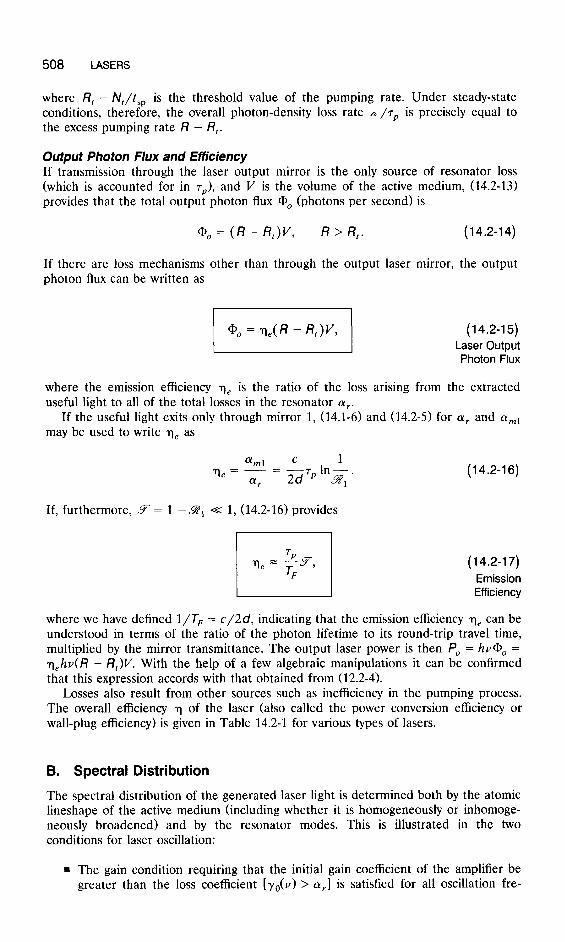
. An intracavity tilted etalon (Fabry-Perot resonator) whose mirror separation d, is much shorter (thinner) than the laser resonator may be used for mode selection (Fig. 14.2-14). M o d es of the etalon have a large spacing c/2d, > B, so that only one etalon mode can fit within the laser amplifier bandwidth. The etalon is designed so that one of its modes coincides with the resonator longitudinal mode exhibiting the highest gain (or any other desired mode). The etalon may be fine-tuned by means of a slight rotation, by changing its temperature, or by slightly changing its width d, with the help of a piezoelectric (or other) trans- ducer. The etalon is slightly tilted with respect to the resonator axis to prevent

Etalon

refl2ikce + I-cdl mirror

Active medium output mirror

I

1 + Laser output

Figure 14.2-14 Longitudinal mode selection by the use of an intracavity etalon. Oscillation occurs at frequencies where a mode of the resonator coincides with an etalon mode; both must, of course, lie within the spectral window where the gain of the medium exceeds the loss.

518 LASERS

(6) 11

(c) 4 Figure 14.2-15 Longitudinal mode selection by use of (a) two coupled resonators (one passive and one active); (6) two coupled active resonators; (c) a coupled resonator-interferometer.

reflections from its surfaces from reaching the resonator mirrors and thereby creating undesired additional resonances. The etalon is usually temperature stabilized to assure frequency stability.

. Multiple-mirror resonators can also be used for mode selection. Several configurations are illustrated in Fig. 14.2-15. Mode selection may be achieved by means of two coupled resonators of different lengths [Fig. 14.2-15(a)]. The resonator in Fig. 14.2-15(b) consists of two coupled cavities, each with its own gain-in essence, two coupled lasers. This is the configuration used for the C3 (cleaved- coupled-cavity) semiconductor laser discussed in Chap. 16. Another technique makes use of a resonator coupled with an interferometer [Fig. 14.2-15(c)]. The theory of coupled resonators and coupled resonator/interferometers is not addressed here.

E. Characteristics of Common Lasers

Laser amplification and oscillation is ubiquitous and can take place in a great variety of media, including solids (crystals, glasses, and fibers), gases (atomic, ionic, molecular, and excimeric), liquids (organic and inorganic solutes), and plasmas (in which x-ray laser action occurs). The active medium can also be provided by the energy levels of an electron in a magnetic field, as in the case of the free electron laser.

Solid-State Lasers In Sec. 13.2C we discussed several solid-state laser amplifiers in some detail: ruby, Nd3+:YAG, Nd3+:glass, and Er 3’:silica fiber. When placed in an optical resonator that provides feedback, all of these materials behave as laser oscillators.

Nd3+:YAG, in particular, enjoys widespread use (see Fig. 13.2-11 for the energy levels of Nd3+:YAG). Its threshold is about an order of magnitude lower than that of ruby by virtue of it being a four-level system. Because it can be optically pumped to its upper laser level by light from a semiconductor laser diode, as shown schematically in Fig. 13.2-8, Nd3+:YAG serves as an efficient compact source of 1.064~pm laser radiation powered by a battery. Nd 3+*YAG crystals with lengths as small as a fraction . of a millimeter operate as single-frequency (microchip) lasers. Furthermore, neodymium laser light can be passed through a second-harmonic generating crystal (see Sec. 19.2A) which doubles its frequency, thereby providing a strong source of radiation at 532 nm in the green.


Because the transitions in Nd3 + arise from inner electrons, which are well shielded from their surroundings, this ionic impurity can, in fact, be made to lase near 1.06 pm in a broad variety of hosts, including glasses of various types, yttrium lithium fluoride (YLF) and yttrium scandium gallium garnet (YSGG). The use of scandium in place of the aluminum in YAG serves to increase the efficiency by about a factor of 2, whereas the gallium aids in the crystal growth. Nd3+ ions may even be dissolved in selenium oxychloride which operates as a liquid Nd 3+ laser. Transitions in other rare-earth ions exhibit similar robustness.

Rare-earth-doped silica fibers can, with proper resonator design, be operated as single-longitudinal-mode lasers (see Fig. 13.2-8). An example is provided by a 5-m-long Er3+:silica fiber laser operated in a Fabry-Perot configuration. A mirror reflectance of 99% at one end and 4% at the other end (simple Fresnel reflection) provides an output of about 8 mW with a semiconductor pump power of 90 mW at 1.46 pm. Alternatively, cavities can be constructed in the form of fiber ring resonators or fiber loop reflectors. Doped silica fiber lasers can also function in pulsed Q-switched and mode-locked configurations (see Sec. 14.3). At 300 K this system behaves as a three-level laser, while at 77 K it behaves as a four-level laser. The distinction is important because there is an optimal fiber length for achieving minimum threshold in a three-level system, whereas in a four-level system the threshold power decreases inversely with the active fiber length.

Aside from ruby, Nd3 +, and Er 3 +, other commonly encountered optically pumped solid-state laser amplifiers and oscillators include alexandrite (Cr 3 +:Al 2 BeO,), which offers a tunable output in the wavelength range between 700 and 800 nm; Ti3+:A1,0, (Ti:sapphire), which is tunable over an even broader range, from 660 to 1180 nm; and Er3+:YAG, which is often operated at 1.66 pm.

Gas Lasers The gas laser is probably the most frequently encountered type of laser oscillator. The red-orange, green, and blue beams of the He-Ne, Ar+, and He-Cd gas lasers, respectively, are by now familiar to many (see Fig. 12.1-3 for the energy levels of He and Ne). The Kr+ laser readily produces hundreds of milliwatts of optical power at wavelengths ranging from 350 nm in the ultraviolet to 647 nm in the red. It can be operated simultaneously on a number of lines to produce “white laser light.” These lasers can all be operated on innumerable other lines. Small He-Ne lasers are so commonplace and inexpensive that they are used by lecturers as pointers and in supermarkets as bar-code readers.

Molecular gas lasers such as CO, (see Fig. 12.1-1 for the energy levels of CO,) and CO, which operate in the middle-infrared region of the spectrum, are highly efficient and can produce copious amounts of power. Indeed, most molecular transitions in the infrared region can be made to lase; even simple water vapor (H,O) lases at many wavelengths in the far infrared.

A gas laser of high current importance in the ultraviolet region is the excimer laser. Excimers (e.g., KrF) exist only in the form of excited electronic states since the constituents are repulsive in the ground state. The lower laser level is therefore always empty, providing a built-in population inversion. Rare-gas halides readily form com- plexes in the excited state because the chemical behavior of an excited rare gas atom is similar to that of an alkali atom, which readily reacts with a halogen.

Liquid Lasers The importance of liquid dye lasers stems principally from their tunability. The active medium of a dye laser is a solution of an organic dye compound in alcohol or water (see Fig. 12.1-4 for a schematic illustration of the energy levels of a dye molecule). Polymethine dyes provide oscillation in the red or near infrared (= 0.7 to 1.5 pm), xanthene dyes lase in the visible (500 to 700 nm), coumarin dyes oscillate in the

520 LASERS

blue-green (400 to 500 nm), and scintillator dyes lase in the ultraviolet region of the spectrum (< 400 nm). Rhodamine-6G dye, for example, can be tuned over the range from 560 to 640 nm.

Plasma X-Ray Lasers A number of different types of x-ray lasers have been operated during the past decade. The difficulty in achieving x-ray laser action stems from several factors. The threshold population difference Nt, according to (14.1-14), is proportional to 1/h27,. It is therefore increasingly difficult to attain threshold as h decreases. Furthermore, it is technically difficult to fabricate high-quality mirrors in the x-ray region because the refractive index does not vary appreciably from material to material. Dielectric mirrors therefore require a very large number of layers, rendering the resonator loss coefficient cy, large and the photon lifetime TV small. Improved x-ray optical components are in the offing, however.

X-ray laser action was apparently first achieved in a dramatic experiment carried out by researchers at the Lawrence Livermore National Laboratory (LLNL) in 1980. An underground nuclear detonation was used to create x-rays, which, in turn, served to pump the atoms in an assembly of metal rods. The x-ray laser pulse was generated before the detonation vaporized the apparatus.

In a series of more controlled experiments at the Princeton Plasma Physics Labora- tory (PPPL) in New Jersey, a solid carbon disk was used as the x-ray laser medium. A 10.6~pm-wavelength CO, laser pulse, of 50 ns duration and 300 J energy, was focused onto the carbon. The infrared laser pulse generated sufficient heat to strip all the electrons away from some of the carbon atoms, thereby creating a plasma of ionized carbon (C6’) and serving as the pump. The plasma was radially confined by the use of a magnetic field. The cooling of the plasma at the termination of the laser pulse led to the capture of electrons in the 4 = 3 orbits of the hydrogen-like C6+ ions, and simultaneously to a dearth of electrons in the 4 = 2 orbits, resulting in a population inversion (see Fig. 12.1-2).

As expected from (12.1-6), the decay of electrons from 4 = 3 to 4 = 2 was accompanied by the emission of x-ray photons of energy

With Z = 6 this corresponds to a photon of energy 68 eV and wavelength A, = (1.24/68) pm = 18.2 nm. These spontaneously emitted photons caused the stimulated emission of x-ray photons from other atoms, resulting in amplified spontaneous emission (ASE). These experiments exhibited a single-pass gain coefficient-length product yd = 6, so that in accordance with (13.1-7) the gain was G = e6. The result was the generation of a 20-ns pulse of soft x-ray ASE with a power of 100 kW, an energy of 2 mJ, and a divergence of 5 mrad.

More recently, the gigantic NOVA 1.06~pm Nd3+:glass laser system at LLNL was used to vaporize thin foils of tantalum and tungsten metal, creating nickel-like Ta45+ and W46+ ions respectively, and producing 250-ps x-ray laser pulses at wavelengths as short as h, = 4.3 nm.

Potential x-ray laser applications include x-ray microlithography for producing the next generation of densely packed semiconductor chips, and the dynamic imaging and holography of individual cellular structures in biological specimens.

Free Electron Lasers The free electron laser (FEL) makes use of a magnetic “wiggler” field, which is produced by a periodic assembly of magnets of alternating polarity. The active medium


is a relativistic electron beam moving in the wiggler field. The electrons are not bound to atoms, but they are nevertheless not truly free since their motion is governed by the wiggler field. The emission wavelength can be tuned over a broad range by changing the electron-beam energy and the magnet period. Depending on their design, FELs can emit at wavelengths that range from the vacuum ultraviolet to the far infrared. Several examples of operating FELs are: the ultraviolet FEL at the University of Paris, which operates near 0.2 pm; the visible FEL at Stanford University (California), which operates in the region from 0.5 to 10 pm; the middle-infrared FEL at the Los Alamos National Laboratory (LANL) in New Mexico, which operates in the region from 9 to 40 pm; and the far-infrared FEL at the University of California at Santa Barbara, which operates in the wavelength band from 400 to 1000 pm.

Tabulation of Selected Laser Transitions In Table 14.2-1 we provide a list, in order of increasing wavelength, of the representa- tive parameters and characteristics of some well-known laser transitions. The broad range of transition wavelengths, overall efficiencies, and power outputs for the different lasers is noteworthy.

The transition cross section, spontaneous lifetime, and atomic linewidth for a number of these laser transitions are listed in Table 13.2-1. The linewidth of the laser

TABLE 14.2-I Typical Characteristics and Parameters for a Number of Well-Known Gas (gh Solid (s), Liquid (I), and Plasma (p) Laser Transitions

Single Mode Approximate Transition 6) or CW Overall output Energy-

Wavelength Multimode or Efficiency Power or Level Laser Medium A0 CM) Pulsed” q(%o)h Energy” Diagram

c6+ (PI 18.2 nm ArF excimer (g) 193 nm KrF excimer (g) 248 nm He-Cd (g) 442 nm Ar+ (g) 515 nm Rhodamine-6G

dye (I) 560-640 nm He-Ne (g) 633 nm Kr+ (8) 647 nm Ruby (s) 694 nm Ti3+:A1203 (s) 0.66-1.18 pm Nd3+:glass (s) 1.06 pm Nd3 +:YAG (s) 1.064 pm KF color

center (s) 1.25-1.45 pm He-Ne (g> 3.39 pm FEL (LANL) 9-40 pm co* w 10.6 pm H,O 6s) 118.7 pm HCN W 336.8 pm

M M M

S/M S/M

S/M S/M S/M

M S/M

M S/M

S/M S/M

M S/M S/M S/M

Pulsed Pulsed Pulsed

cw cw

1o-5

0.1 0.05

2 mJ Fig. 12.1-2 500 mJ 500 mJ 10 mW 10 w

cw cw cw

Pulsed cw

Pulsed cw

cw 0.005 500 mW cw 0.05 1 mW Fig. 12.1-3

Pulsed 0.5 1 mJ cw 10. 100 W Fig. 12.1-1 cw 0.001 10 /Lw cw 0.001 1 mW

0.005 0.05 0.01 0.1 0.01

0.5

100 mW Fig. 12.1-4 1 mW Fig. 12.1-3

500 mW 5 J Fig. 13.2-9

10 w 50 J Fig. 13.2-11 10 W Fig. 13.2-11

522 LASERS

output is generally many orders of magnitude smaller than the atomic linewidths given in Table 13.2-1; this is because of the additional frequency selectivity imposed by the optical resonator. Some laser systems cannot sustain a continuous population inversion and therefore operate only in a pulsed mode.

14.3 PULSED LASERS

A. Methods of Pulsing Lasers

The most direct method of obtaining pulsed light from a laser is to use a continuous- wave (CW) laser in conjunction with an external switch or modulator that transmits the light only during selected short time intervals. This simple method has two distinct disadvantages, however. First, the scheme is inefficient since it blocks (and therefore wastes the light) energy during the off-time of the pulse train. Second, the peak power of the pulses cannot exceed the steady power of the CW source, as illustrated in Fig. 14.3-l(a).

More efficient pulsing schemes are based on turning the laser itself on and off by means of an internal modulation process, designed so that energy is stored during the off-time and released during the on-time. Energy may be stored either in the resonator, in the form of light that is periodically permitted to escape, or in the atomic system, in the form of a population inversion that is released periodically by allowing the system to oscillate. These schemes permit short laser pulses to be generated with peak powers far in excess of the constant power deliverable by CW lasers, as illustrated in Fig. 14.3-l(b).

Four common methods used for the internal modulation of laser light are: gain switching, Q-switching, cavity dumping, and mode locking. These are considered in turn.

Gain Switching In this rather direct approach, the gain is controlled by turning the laser pump on and off (Fig. 14.3-2). In the flashlamp-pumped pulsed ruby laser, for example, the pump (flashlamp) is switched on periodically for brief periods of time by a sequence of electrical pulses. During the on-times, the gain coefficient exceeds the loss coefficient and laser light is produced. Most pulsed semiconductor lasers are gain switched because it is easy to modulate the electric current used for pumping, as discussed in Chap. 16. The laser-pulse rise and fall times achievable with gain switching are determined in Sec. 14.3B.

Modulator Modulator

Peak power \,

t t (a) (b)

Figure 14.3-l Comparison of pulsed laser outputs achievable with (a) an external modulator, and (b) an internal modulator.

PULSED LASERS 523

-- t

Pump 1

Figure 14.3-2 Gain switching.

Q-S witching In this scheme, the laser output is turned off by increasing the resonator loss (spoiling the resonator quality factor Q) periodically with the help of a modulated absorber insider the resonator (Fig. 14.3-3). Thus Q-switching is loss switching. Because the pump continues to deliver constant power at all time, energy is stored in the atoms in the form of an accumulated population difference during the off (high-loss)-times. When the losses are reduced during the on-times, the large accumulated population difference is released, generating intense (usually short) pulses of light. An analysis of this method is provided in Sec. 14.3C.

Cavity Dumping This technique is based on storing photons (rather than a population difference) in the resonator during the off-times, and releasing them during the on-times. It differs from Q-switching in that the resonator loss is modulated by altering the mirror transmittance (see Fig. 14.3-4). Th e system operates like a bucket into which water is poured from a hose at a constant rate. After a period of time of accumulating water, the bottom of the bucket is suddenly removed so that the water is “dumped.” The bucket bottom is subsequently returned and the process repeated. A constant flow of water is therefore converted into a pulsed flow. For the cavity-dumped laser, of course, the bucket represents the resonator, the water hose represents the constant pump, and the bucket bottom represents the laser output mirror. The leakage of light from the resonator, including useful light, is not permitted during the off-times. This results in negligible resonator losses, thereby increasing the optical power inside the laser resonator. Photons are stored in the resonator and cannot escape. The mirror is suddenly removed altogether (e.g., by rotating it out of alignment), increasing its transmittance to 100% during the on-times. As the accumulated photons leave the resonator, the sudden increase in the loss arrests the oscillation. The result is a strong pulse of laser light. The analysis for cavity dumping is not provided here inasmuch as it is closely related to that of Q-switching. This is because the variation of the gain and loss with time are similar, as may be seen by comparing Fig. 14.3-4 with Fig. 14.3-3.

Modulated absorber

Figure 14.3-3 Q-switching.

524 LASERS

Gain

Loss

Mirror transmittance

Laser output

Figure 14.3-4 Cavity dumping. One of the mirrors is removed altogether to dump the stored photons as useful light.

Mode Locking Mode locking is distinct from the previous three techniques. Pulsed laser action is attained by coupling together the modes of a laser and locking their phases to each other. For example, the longitudinal modes of a multimode laser, which oscillate at frequencies that are equally separated by the intermodal frequency c/2d, may be made to behave in this fashion. When the phases of these components are locked together, they behave like the Fourier components of a periodic function, and therefore form a periodic pulse train. The coupling of the modes is achieved by periodically modulating the losses inside the resonator. Mode locking is examined in Sec. 14.3D.

*B. Analysis of Transient Effects

An analytical description of the operation of pulsed lasers requires an understanding of the dynamics of the laser oscillation process, i.e., the time course of laser oscillation onset and termination. The steady-state solutions presented earlier in the chapter are inadequate for this purpose. The lasing process is governed by two variables: the number of photons per unit volume in the resonator, n(t), and the atomic population difference per unit volume, N(t) = N,(t) - N,(t); both are functions of the time t.

Rate Equation for the Photon-Number Density The photon-number density n is governed by the rate equation

(14.3-1)

The first term represents photon loss arising from leakage from the resonator, at a rate given by the inverse photon lifetime l/rp. The second term represents net photon gain, at a rate A/WI:, arising from stimulated emission and absorption. IA$ = +(v) = c&a(v) is the probability density for induced absorption/emission. Spontaneous emission is assumed to be small. With the help of the relation N, = cu,/a(v) = ~/CT&), where A/, is the threshold population difference [see (14.1-13)], we write (T(V) = l/c~,N,,

PULSED LASERS 525

from which

Substituting this into (14.3-1) provides a simple differential equation for the photon number density n ,

dn n N/Z -= --+---* dt 7P Nt rp

I I

(14.3-2) Photon-Number

Rate Equation

As long as N > N,, d n /dt will be positive and n will increase. When steady state (d n /dt = 0) is reached, N = N,.

Rate Equation for the Population Difference The dynamics of the population difference N(t) depends on the pumping configuration. A three-level pumping scheme (see Sec. 13.2B) is analyzed here. The rate equation for the population of the upper energy level of the transition is, according to (13.2~5),

dN2 - = R - ” - Wi( N, - N,), dt SP

(14.3-3)

where it is assumed that r2 = tsp. R is the pumping rate, which is assumed to be independent of the population difference N. Denoting the total atomic number density N, + N, by N,, so that N, = (N, - N)/2 and N, = (N, + N)/2, we obtain a differential equation for the population difference N = N, - N,,

dN N, N -=---- dt tsp tsp

2WiN, (14.3-4)

where the small-signal population difference N, = 2Rt,, - N, [see (13.2-22)]. Substi- tuting the relation Wi =IZ /Ntrp obtained above into (14.3-4) then yields

(Three-Level System)

The third term on the right-hand side of (14.3-5) is twice the second term on the right-hand side of (14.3-2), and of opposite sign. This reflects the fact that the generation of one photon by an induced transition reduces the population of level 2 by one atom while increasing the population of level 1 by one atom, thereby decreasing the population difference by two atoms.

Equations (14.3-2) and (14.3-5) are coupled nonlinear differential equations whose solution determines the transient behavior of the photon number density n(t) and the population difference N(t). Setting dN/dt = 0 and dn /dt = 0 leads to N = N,

526 LASERS

and n = (N, - N,)(7p/2tsp). These are indeed the steady-state values of N and n obtained previously, as is evident from (14.2-12) with 7S = 2tsp, as provided by (13.2-23) for a three-level pumping scheme.

EXERCISE 14.3- 1

Population-Difference Rate Equafion for a Four-Level System. Obtain the population-difference rate equation for a four-level system for which 71 -=c t,,. Explain the absence of the factor of 2 that appears in (14.3-5).

Gain Switching Gain switching is accomplished by turning the pumping rate R on and off, this, in turn, is equivalent to modulating the small-signal population difference A/, = 2Rt,, - N,. A schematic illustration of the typical time evolution of the population difference N(t) and the photon-number density n(t), as the laser is pulsed by varying N, is provided in Fig. 14.3-5. The following regimes are evident in the process:

. For t < 0, the population difference N(t) = N,,, lies below the threshold Nt and oscillation cannot occur.

. The pump is turned on at t = 0, which increases N, from a value N,, below threshold to a value A/,, above threshold in step-function fashion. The population difference N(t) begins to increase as a result. As long as N(t) < N,, however, the photon-number density n = 0. In this region (14.3-5) therefore becomes dN/dt = W, - N)/&,, indicating that N(t) grows exponentially toward its equilibrium value Nob with time constant t,,.

. Once N(t) crosses the threshold N,, at t = t,, laser oscillation begins and n(t) increases. The population inversion then begins to deplete so that the rate of

N0b

Nt

NOLl

-

Photon number density

Figure 14.3-5 Variation of the population difference N(t) and the photon-number density n(t) with time, as a square pump pulse results in A/, suddenly increasing from a low value IV,, to a high value N,,, and then decreasing back to a low value N,,.

PULSED LASERS 527

increase of N(t) slows. As n(t) becomes larger, the depletion becomes more effective so that N(t) begins to decay toward A/,. N(t) finally reaches N,, at which

- time n(t) reaches its steady-state value. n The pump is turned off at time t = t,, which reduces A/, to its initial value A/,,.

N(t) and n(t) decay to the values A/,, and 0, respectively.

The actual profile of the buildup and decay of n(t) is obtained by numerically solving (14.3-2) and (14.3-5). The precise shape of the solution depends on t,,, rp, N,, as well as on N,, and N,, (see Problem 14.3-1).

*C. Q-Switching

Q-switched laser pulsing is achieved by switching the resonator loss coefficient (Y, from a large value during the off-time to a small value during the on-time. This may be accomplished in any number of ways, such as by placing a modulator that periodically introduces large losses in the resonator. Since the lasing threshold population difference N, is proportional to the resonator loss coefficient (Y, [see (14.1-12) and (14.1-91, the result of switching cy,. is to decrease Nt from a high value N,, to a low value N,,, as illustrated in Fig. 14.3-6. In Q-switching, therefore, N, is modulated while No remains fixed, whereas in gain switching N, is modulated while Nt remains fixed (see Fig. 14.3-5). The population and photon-number densities behave as follows:

. At t = 0, the pump is turned on so that N, follows a step function. The loss is maintained at a level that is sufficiently high (N, = Nta > No) so that laser oscillation cannot begin. The population difference N(t) therefore builds up (with time constant ts,>. Although the medium is now a high-gain amplifier, the loss is sufficiently large so that oscillation is prevented.

n At t = t,, the loss is suddenly decreased so that N, diminishes to a value N,, < N,. Oscillation therefore begins and the photon-number density rises sharply. The presence of the radiation causes a depletion of the population inversion (gain saturation) so that N(t) begins to decrease. When N(t) falls below N,,, the loss again exceeds the gain, resulting in a rapid decrease of the photon-number density (with a time constant of the order of the photon lifetime rp).

Nta -----------__ 1 r---------i r-------- Loss I I I

Nt Ntb

Pump

Population mversion

Photon number density

Figure 14.3-6 Operation of a Q-switched laser. Variation of the population threshold N, (which is proportional to the resonator loss), the pump parameter N,, the population difference N(t), and the photon number n(t).

528 LASERS

n At t = t,, the loss is reinstated, insuring the availability of a long period of population-inversion buildup to prepare for the next pulse. The process is repeated periodically so that a periodic optical pulse train is generated.

We now undertake an analysis to determine the peak power, energy, width, and shape of the optical pulse generated by a Q-switched laser in the steady pulsed state. We rely on the two basic rate equations (14.3-2) and (14.3-5) for n(t) and N(t), respectively, which we solve during the on-time ti to tf indicated in Fig. 14.3-6. The problem can, of course, be solved numerically. However, it simplifies sufficiently to permit an analytic solution if we assume that the first two terms of (14.3-5) are negligible. This assumption is suitable if both the pumping and the spontaneous emission are negligible in comparison with the effects of induced transitions during the short time interval from ti to tf. This approximation turns out to be reasonable if the width of the generated optical pulse is much shorter than t,,. When this is the case, (14.3-2) and (14.3-5) become

dN - = -2Lk dt Nt rp *

(14.3-6)

(14.3-7)

These are two coupled differential equations in n(t) and N(t) with initial conditions n = 0 and N = Ni at t = ti. Throughout the time interval from ti to tf, Nt is fixed at its low value N,,.

Dividing (14.3-6) by (14.3-7), we obtain a single differential equation relating n and N,

(14.3-8)

which we integrate to obtain

AT= $N, ln( N) - +N + constant. (14.3-9)

Using the initial condition n = 0 when N = Ni finally leads to

n = iNt lni - t(N - Ni). 1

(14.3-10)

Pulse Power According to (14.2-10) and (14.2-3), the internal photon-flux density (comprising both directions) is given by C$ =nc, whereas the external photon-flux density emerging from mirror 1 (which has transmittance 7) is 4, = $YIZC. Assuming that the photon-flux

PULSED LASERS 529

density is uniform over the cross-sectional area A of the emerging beam, the corresponding optical output power is

(14.3-11)

where V = Ad is the volume of the resonator. According to (14.2-17), if Y -=K 1, the fraction of the resonator loss that contributes to useful light at the output is qe = 9-k/2d)Tp, so that we obtain

6Z?V PO = q,hv-.

7P

(14.3-12)

Equation (14.3-12) is easily interpreted since the factor IZV/T~ is the number of photons lost from the resonator per unit time.

Peak Pulse Power As discussed earlier and illustrated in Fig. 14.3-6, n reaches its peak value np when N = N, = N,,. This is corroborated by setting dn /dt = 0 in (14.3-6), which leads immediately to N = N,. Substituting this into (14.3-10) therefore provides

Using this result in conjunction with (14.3-11) gives the peak power

Pp = hvY$Vn P’

(14.3-14)

(14.3-13)

When Ni z+ N,, as must be the case for pulses of large peak power, N,/N, -C 1, whereupon (14.3-13) gives

n = P $‘J,, (14.3-X)

The peak photon-number density is then equal to one-half the initial population density difference. In this case, the peak power assumes the particularly simple form

(14.3-16) Peak Pulse Power

Pulse Energy The pulse energy is given by

E = ItfPo dt, t,

which, in accordance with Eq. (14.3-111, can be written as

E = h,++(t) dt = hvF&V/~N&(t)-$ dN. t, I

(14.3-17)

530 LASERS

Using (14.3-7) in (14.3-17), we obtain

which integrates to

(14.3-18)

(14.3-19)

The final population difference Nf is determined by setting n = 0 and N = Nf in (14.3-10) which provides

(14.3-20)

Substituting this into (14.3-19) gives

When Ni * Nf, E =: ~hv~(c/2d)VT~Ni, as expected. It remains to solve (14.3-20) for Nf. One approach is to rewrite it in the form Y exp( -Y) = X exp( -X), where X = Ni/N, and Y = Nf/N, Given X = Ni/N,, we can easily solve for Y numerically or by using the graph provided in Fig. 14.3-7.

Pulse Width A rough estimate of the pulse width is the ratio of the pulse energy to the peak pulse power. Using (14.3-13), (14.3-14), and (14.3-21), we obtain

When Ni Z+ N, and Ni Z+ Nf, rputse = rP.

x1x2 y2 y1 x

Figure 14.3-7 Graphical construction for determining Nf from /Vi, where X = NJ/V, and Y = Nf/NI. For X = X, the ordinate represents the value X, exp( -XI>. Since the corresponding solution YI obeys YI exp( - YI> = X, exp( -XI), it must have the same value of the ordinate.

PULSED LASERS 531

Figure 14.3-8 Typical Q-switched pulse shapes obtained from numerical integration of the approximate rate equations. The photon-number density n(t) is normalized to the threshold population difference Nl = Nrb and the time t is normalized to the photon lifetime TV. The pulse narrows and achieves a higher peak value as the ratio Ni/N, increases. In the limit Ni/N, s 1, the peak value of n(t) approaches ~Ni.

Pulse Shape The optical pulse shape, along with all of the pulse characteristics described above, can be determined by numerically integrating (14.3-6) and (14.3-7). Examples of the resulting pulse shapes are shown in Fig. 14.3-8.

EXERCISE 14.3-2

Pulsed Ruby Laser. Consider the ruby laser discussed in Exercise 14.1-1 on page 501. If the laser is now Q-switched so that at the end of the pumping cycle (at t = t, in Fig. 14.3-6) the population difference Ni = 6N,, use Fig. 14.3-8 to estimate the shape of the laser pulse, its width, peak power, and total energy.

D. Mode Locking

A laser can oscillate on many longitudinal modes, with frequencies that are equally separated by the intermodal spacing VF = c/2d. Although these modes normally oscillate independently (they are then called free-running modes), external means can be used to couple them and lock their phases together. The modes can then be regarded as the components of a Fourier-series expansion of a periodic function of time of period TF = l/uF = 2d/c, in which case they constitute a periodic pulse train. After examining the properties of a mode-locked laser pulse train, we discuss methods of locking the phases of the modes together.

532 LASERS

Properties of a Mode-Locked Pulse Train If each of the laser modes is approximated by a uniform plane wave propagating in the z direction with a velocity c = co/n, we may write the total complex wavefunction of the field in the form of a sum:

U(z, t) = CA exp $2 q 4 [ Y(t - r,]? (14.3-23)

where

vq = u() + qvF, q = 0, f 1, f 2,. . . (14.3-24)

is the frequency of mode q, and A, is its complex envelope. For convenience we assume that the q = 0 mode coincides with the central frequency v. of the atomic lineshape. The magnitudes IA,/ may be determined from knowledge of the spectral profile of the gain and the resonator loss (see Sec. 14.2B). Since the modes interact with different groups of atoms in an inhomogeneously broadened medium, their phases arg{A,} are random and statistically independent.

Substituting (14.3-24) into (14.3-23) provides

U(z,t) =d(t - +q+%yo - :)I, where the complex envelope s’(t) is the function

jq2rt d(t) = CA,exp 7

4 ( i F

and

(14.3-26)

(14.3-27)

The complex envelope d(t) in (14.3-26) is a periodic function of the period TF, and dt - z/c) is a periodic function of z of period cTF = 2d. If the magnitudes and phases of the complex coefficients A, are properly chosen, d(t) may be made to take the form of periodic narrow pulses.

Consider, for example, M modes (q = 0, f 1, . . . , f S, so that M = 2s + l), whose complex coefficients are all equal, A, = A, q = 0, + 1, . . . , f S. Then

d(t) = A i exp q= -s

=A 5 xs+l -p XS+f _ x-S-f

x4 =A =A x-l I ,

q= -s xLx 2

where x = exp( j2rt/TF) (see Sec. 2.6B for more details). After a few algebraic manipulations, a?(t) can be cast in the form

d(t) =A sin( M7r t/TF)

sin( 7r t/T,) -

PULSED LASERS 533

Intensity

Figure 14.3-9 Intensity of the periodic pulse train resulting from the sum of A4 laser modes of equal magnitudes and phases. Each pulse has a width that is M times smaller than the period r, and a peak intensity that is M times greater than the mean intensity.

The optical intensity is then given by I(t, z) = Id(t - z/c)12 or

qt, 2) = IAl sin2 [ M7r( t - z/c)/TF]

sin2 [7r(t - z/c)/T,] * (14.3-28)

As illustrated in Fig. 14.3-9, this is a periodic function of time. The shape of the mode-locked laser pulse train is therefore dependent on the

number of modes M, which is proportional to the atomic linewidth Av. The pulse width 7pulse is therefore inversely proportional to the atomic linewidth Au. If M = Av/vF, then 7pulse = T,/M = l/Au. Because Au can be quite large, very narrow mode-locked laser pulses can be generated. The ratio between the peak and mean intensities is equal to the number of modes M, which can also be quite large.

The period of the pulse train is TF = 2d/c. This is just the time for a single round trip of reflection within the resonator. Indeed, the light in a mode-locked laser can be regarded as a single narrow pulse of photons reflecting back and forth between the mirrors of the resonator (see Fig. 14.3-10). At each reflection from the output mirror, a fraction of the photons is transmitted in the form of a pulse of light. The transmitted

Optical switch

Figure 14.3-10 The mode-locked laser pulse reflects back and forth between the mirrors of the resonator. Each time it reaches the output mirror it transmits a short optical pulse. The transmitted pulses are separated by the distance 2d and travel with velocity c. The switch opens only when the pulse reaches it and only for the duration of the pulse. The periodic pulse train is therefore unaffected by the presence of the switch. Other wave patterns, however, suffer losses and are not permitted to oscillate.

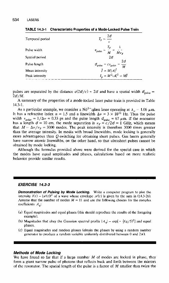
534 LASERS

TABLE 14.3-1 Characteristic Properties of a Mode-Locked Pulse Train

Temporal period

Pulse width

TF= 2d c

TF 1 Tpulse = G = K

F

Spatial period

Pulse length

Mean intensity Peak intensity

2d 2d

d pulse = CTpulse = - A4

r = MIA12 I, = M2)A12 = MI

pulses are separated by the distance c(2d/c) = 2d and have a spatial width dpulse = 2d/M.

A summary of the properties of a mode-locked laser pulse train is provided in Table 14.3-1.

As a particular example, we consider a Nd3+:glass laser operating at A, = 1.06 pm. It has a refractive index n = 1.5 and a linewidth Au = 3 X 1012 Hz. Thus the pulse width 7pulse = l/Au = 0.33 ps and the pulse length dpulse = 67 pm. If the resonator has a length d = 10 cm, the mode separation is v)F = c/2d = 1 GHz, which means that M = ALJ/V~ = 3000 modes. The peak intensity is therefore 3000 times greater than the average intensity. In media with broad linewidths, mode locking is generally more advantageous than Q-switching for obtaining short pulses. Gas lasers generally have narrow atomic linewidths, on the other hand, so that ultrashort pulses cannot be obtained by mode locking.

Although the formulas provided above were derived for the special case in which the modes have equal amplitudes and phases, calculations based on more realistic behavior provide similar results.

EXERCISE 14.3-3

Demonstration of Pulsing by Mode Locking. Write a computer program to plot the intensity I(t) = Id( of a wave whose envelope d(t) is given by the sum in (14.3-26). Assume that the number of modes M = 11 and use the following choices for the complex coefficients A,:

(a) Equal magnitudes and equal phases (this should reproduce the results of the foregoing example).

(b) Magnitudes that obey the Gaussian spectral profile IA,1 = exp[ - i(q/5)2] and equal phases.

(c) Equal magnitudes and random phases (obtain the phases by using a random number generator to produce a random variable uniformly distributed between 0 and 277).

Methods of Mode Locking We have found so far that if a large number M of modes are locked in phase, they form a giant narrow pulse of photons that reflects back and forth between the mirrors of the resonator. The spatial length of the pulse is a factor of M smaller than twice the

PULSED LASERS 535

resonator length. The question that remains is how the modes can be locked together so that they have the same phase. This can be accomplished with the help of a modulator or switch placed inside the resonator, as we now show.

Suppose that an optical switch (e.g., an electro-optic or acousto-optic switch, as discussed in Chaps. 18, 20, and 21) is placed inside the resonator, which blocks the light at all times, except when the pulse is about to cross it, whereupon it opens for the duration of the pulse (Fig. 14.3-10). Since the pulse itself is permitted to pass, it is not affected by the presence of the switch and the pulse train continues uninterrupted. In the absence of phase locking, the individual modes have different phases that are determined by the random conditions at the onset of their oscillation. If the phases happen, by accident, to take on equal values, the sum of the modes will form a giant pulse that would not be affected by the presence of the switch. Any other combination of phases would form a field distribution that is totally or partially blocked by the switch, which adds to the losses of the system. Therefore, in the presence of the switch, only the case where the modes have equal phases can lase. The laser waits for the lucky accident of such phases, but once the oscillations start, they continue to be locked.

The problem can also be examined mathematically. An optical field must satisfy the wave equation with the boundary conditions imposed by the presence of the switch. The multimode optical field of (14.3-23) does indeed satisfy the wave equation for any combination of phases. The case of equal phases also satisfies the boundary conditions imposed by the switch; therefore, it must be a unique solution.

A passive switch such as a saturable absorber may also be used for mode locking. A saturable absorber (see Sec. 13.3B) is a medium whose absorption coefficient decreases as the intensity of the light passing through it increases; thus it transmits intense pulses with relatively little absorption and absorbs weak ones. Oscillation can therefore occur only when the phases of the different modes are related to each other in such a way that they form an intense pulse which can then pass through the switch. Active and passive switches are also used for the mode locking of homogeneously broadened media.

Examples of Mode-Locked Lasers Table 14.3-2 is a list, in order of increasing observed pulse width, of some mode-locked laser media. A broad range of observed pulse widths is represented. The observed pulse widths, which for a given medium can vary greatly, depend on the method used to achieve mode locking. Rhodamine-6G dye lasers, for example, can be constructed in a colliding pulse mode (CPM) ring-resonator configuration. The oppositely traveling ultrashort laser pulses collide at a very thin jet of dye serving as a saturable absorber.

TABLE 14.3-2 Typical Observed Pulse Widths for a Number of Homogeneously (HI and Inhomogeneously (I) Broadened, Mode-Locked Lasers

Laser Medium

Transition Linewidth’ Av

Calculated Pulse Width

Tpulse = l/Av Observed

Pulse Width

Ti’+:AI,O, H Rhodamine-6G dye H/I Nd” +:glass I Er 3 +:silica fiber WI Ruby H Nd” +:YAG H Ar+ I He-Ne I co2 I

100 THz 10 fs 5 THz 200 fs 3 THz 333 fs 4 THz 250 fs

60 GHz 16 ps 120 GHz 8 PS 3.5 GHz 286 ps 1.5 GHz 667 ps 60 MHz 16 ns

30 fs 500 fs 500 fs

7 PS 10 ps 50 ps

150 ps 600 ps 20 ns

“The transition linewidths Au are obtained from Table 13.2-1.

536 LASERS

Only during the brief time that the optical pulses pass each other in the thin absorber is the intensity increased and the loss minimized. Proper positioning of the active medium relative to the saturable absorber can give rise to pulse widths as low as 25 fs. In a conventional configuration, the pulse width is far greater (= 500 fs).

READING LIST

Books and Articles on Laser Theory See also the reading list in Chapter 13.

Books on Lasers C. A. Brau, Free-Electron Lasers, Academic Press, Orlando, FL, 1990. F. P. Schafer, ed., Dye Lasers, Springer-Verlag, New York, 3rd ed. 1990. R. C. Elton, X-Ray Lasers, Academic Press, Orlando, FL, 1990. N. G. Basov, A. S. Bashkin, V. I. Igoshin, A. N. Oraevsky, and A. A. Shcheglov, Chemical Lasers,

Springer-Verlag, New York, 1990. P. K. Das, Lasers and Optical Engineering, Springer-Verlag, New York, 1990. A. A. Kaminskii, Laser Crystals, Springer-Verlag, New York, 2nd ed. 1990. N. G. Douglas, Millimetre and Submillimetre Lasers, Springer-Verlag, New York, 1989. P. K. Cheo, ed., Handbook of Solid-State Lasers, Marcel Dekker, New York, 1988. P. K. Cheo, ed., Handbook of Molecular Lasers, Marcel Dekker, New York, 1987. L. F. Mollenauer and J. C. White, eds., Tunable Lasers, Springer-Verlag, Berlin, 1987. T. C. Marshall, Free Electron Lasers, Macmillan, New York, 1985. P. Hammerling, A. B. Budgor, and A. Pinto, eds., Tunable Solid State Lasers, Springer-Verlag,

New York, 1985. C. K. Rhodes, ed., Excimer Lasers, Springer-Verlag, Berlin, 2nd ed. 1984. G. Brederlow, E. Fill, and K. J. Witte, The High-Power Iodine Laser, Springer-Verlag, Berlin,

1983. D. C. Brown, High Peak Power Nd:Glass Laser Systems, Springer-Verlag, Berlin, 1981. S. A. Losev, Gasdynamic Laser, Springer-Verlag, Berlin, 1981. A. L. Bloom, Gas Lasers, R. E. Krieger, Huntington, NY, 1978. E. R. Pike, ed., High-Power Gas Lasers, Institute of Physics, Bristol, England, 1975. C. S. Willett, Introduction to Gas Lasers: Population Inversion Mechanisms, Pergamon Press, New

York, 1974. R. J. Pressley, Handbook of Lasers, Chemical Rubber Company, Cleveland, OH, 1971. D. C. Sinclair and W. E. Bell, Gas Laser Technology, Holt, Rinehart and Winston, New York,

1969. L. Allen and D. G. C. Jones, Principles of Gas Lasers, Plenum Press, New York, 1967. C. G. B. Garrett, Gas Lasers, McGraw-Hill, New York, 1967. W. V. Smith and P. P. Sorokin, The Laser, McGraw-Hill, New York, 1966.

Books on Laser Applications F. J. Duarte and L. W. Hillman, Dye Laser Principles with Applications, Academic Press, Orlando,

FL, 1990. P. G. Cielo, Optical Techniques for Industrial Inspection, Academic Press, New York, 1988. W. Guimaraes, C. T. Lin, and A. Mooradian, Lasers and Applications, Springer-Verlag, Berlin,

1987. H. Koebner, Industrial Applications of Lasers, Wiley, New York, 1984. W. W. Duley, Laser Processing and Analysis of Materials, Plenum Press, New York, 1983.

READING LIST 537

H. M. Muncheryan, Principles and Practice of Laser Technology, Tab Books, Blue Summit, PA, 1983.

F. Durst, A. Mellino, and J. H. Whitelaw, Principles and Practice of Laser-Doppler Anemometry, Academic Press, New York, 1981.

L. E. Drain, The Laser Doppler Technique, Wiley, New York, 1980. M. J. Beesley, Lasers and Their Applications, Halsted Press, New York, 1978. J. F. Ready, Industrial Applications of Lasers, Academic Press, New York, 1978. W. E. Kock, Engineering Applications of Lasers and Holography, Plenum Press, New York, 1975. F. T. Arecchi and E. 0. Schulz-Dubois, eds., Laser Handbook, vol. 2, North-Holland/Elsevier,

Amsterdam/New York, 1972. S. S. Charschan, ed., Lasers in Industry, Van Nostrand Reinhold, New York, 1972. J. W. Goodman and M. Ross, eds., Laser Applications, ~01s. l-5, Academic Press, New York,

1971-1984. S. L. Marshall, ed., Laser Technology and Applications, McGraw-Hill, New York, 1968. D. Fishlock, ed., A Guide to the Laser, Elsevier, New York, 1967.

Special Journal Issues Special issue on laser technology, Lincoln Laboratory Journal, vol. 3, no. 3, 1990. Special issue on novel laser system optics, Journal of the Optical Society of America B, vol. 5, no.

9, 1988. Special issue on solid-state lasers, IEEE Journal of Quantum Electronics, vol. QE-24, no. 6, 1988. Special issue on nonlinear dynamics of lasers, Journal of the Optical Society of America B, vol. 5,

no. 5, 1988. Special issue on lasers in biology and medicine, IEEE Journal of Quantum Electronics, vol.

QE-23, no. 10, 1987. Special issue on free electron lasers, IEEE Journal of Quantum Electronics, vol. QE-23, no. 9,

1987. Special issue on the generation of coherent XUV and soft-X-ray radiation, Journal of the Optical

Society of America B, vol. 4, no. 4, 1987. Special issue on solid-state laser materials, Journal of the Optical Society of America B, vol. 3, no.

1, 1986. Special issue: “Twenty-five years of the laser,” Optica Acta (Journal of Modern Optics), vol. 32,

no. 9/10, 1985. Special issue on ultrasensitive laser spectroscopy, Journal of the Optical Society of America B, vol.

2, no. 9, 1985. Third special issue on free electron lasers, IEEE Journal of Quantum Electronics, vol. QE-21, no.

7, 1985. Special issue on infrared spectroscopy with tunable lasers, Journal of the Optical Society of

America B, vol. 2, no. 5, 1985. Special issue on lasers in biology and medicine, IEEE Journal of Quantum Electronics, vol.

QE-20, no. 12, 1984. Centennial issue, IEEE Journal of Quantum Electronics, vol. QE-20, no. 6, 1984. Special issue on laser materials interactions, IEEE Journal of Quantum Electronics, vol. QE-17,

no. 10, 1981. Special issue on free electron lasers, IEEE Journal of Quantum Electronics, vol. QE-17, no. 8,

1981. Special issue on laser photochemistry, IEEE Journal of Quantum Electronics, vol. QE-16, no. 11,

1980. Special issue on excimer lasers, IEEE Journal of Quantum Electronics, vol. QE-15, no. 5, 1979. Special issue on quantum electronics, Proceedings of the IEEE, vol. 51, no. 1, 1963.

538 LASERS

Articles E. Desurvire, Erbium-Doped Fiber Amplifiers for New Generations of Optical Communication

Systems, Optics & Photonics News, vol. 2, no. 1, pp. 6-11, 1991. K.-J. Kim and A. Sessler, Free-Electron Lasers: Present Status and Future Prospects, Science,

vol. 250, pp. 88-93, 1990. G. New, Femtofascination, Physics World, vol. 3, no. 7, pp. 33-37, 1990. P. F. Moulton, Ti: Sapphire Lasers: Out of the Lab and Back In Again, Optics & Photonics News,

vol. 1, no. 8, pp. 20-23, 1990. R. D. Petrasso, Plasmas Everywhere, Nature, vol. 343, pp. 21-22, 1990. S. Suckewer and A. R. DeMeo, Jr., X-Ray Laser Microscope Developed at Princeton, Princeton

Plasma Physics Laboratory Digest, May 1989. H. P. Freund and R. K. Parker, Free-Electron Lasers, Scientific American, vol. 260, no. 4, pp.

84-89, 1989.

P. Urquhart, Review of Rare Earth Doped Fibre Lasers and Amplifiers, Institution of Electrical Engineers Proceedings-Part J, vol. 135, pp. 385-407, 1988.

D. L. Matthews and M. D. Rosen, Soft X-Ray Lasers, Scientific American, vol. 259, no. 6, pp. 86-91, 1988.

C. A. Brau, Free-Electron Lasers, Science, vol. 239, pp. 1115-1121, 1988. R. L. Byer, Diode Laser-Pumped Solid-State Lasers, Science, vol. 239, pp. 742-747, 1988. J. A. Pasour, Free-Electron Lasers, IEEE Circuits and Devices Magazine, vol. 3, no. 2, pp. 55-64,

1987. J. G. Eden, Photochemical Processing of Semiconductors: New Applications for Visible and

Ultraviolet Lasers, IEEE Circuits and Devices Magazine, vol. 2, no. 1, pp. 18-24, 1986. J. F. Holzricher, High-Power Solid-State Lasers, Nature, vol. 316, pp. 309-314, 1985. W. L. Wilson, Jr., F. K. Tittel, and W. Nighan, Broadband Tunable Excimer Lasers, IEEE

Circuits and Devices Magazine, vol. 1, no. 1, pp. 55-62, 1985. P. Sprangle and T. Coffey, New Sources of High-Power Coherent Radiation, Physics Today, vol.

37, no. 3, pp. 44-51, 1984. A. L. Schawlow, Spectroscopy in a New Light, (Nobel lecture), Reviews of Modern Physics, vol. 54,

pp. 697-707, 1982. P. W. Smith, Mode Selection in Lasers, Proceedings of the IEEE, vol. 60, pp. 422-440, 1972. L. Allen and D. G. C. Jones, Mode Locking in Gas Lasers, in Progress in Optics, vol. 9, E. Wolf,

ed., North-Holland, Amsterdam, 1971. P. W. Smith, Mode-Locking of Lasers, Proceedings of the IEEE, vol. 58, pp. 1342-1359, 1970. D. R. Herriott, Applications of Laser Light, Scientific American, vol. 219, no. 3, pp. 141-156,

1968. C. K. N. Patel, High-Power Carbon Dioxide Lasers, Scientific American, vol. 219, no. 2, pp.

22-33, 1968.

A. Lempicki and H. Samelson, Liquid Lasers, Scientific American, vol. 216, no. 6, pp. 80-90, 1967.

PROBLEMS

14.2-1 Number of Longitudinal Modes. An Arf-ion laser has a resonator of length 100 cm. The refractive index n = 1. (a) Determine the frequency spacing vF between the resonator modes. (b) Determine the number of longitudinal modes that the laser can sustain if the FWHM Doppler-broadened linewidth is Av, = 3.5 GHz and the loss coefficient is half the peak small-signal gain coefficient.

PROBLEMS 539

(c) What would the resonator length d have to be to achieve operation on a single longitudinal mode? What would that length be for a CO, laser that has a much smaller Doppler linewidth Av, = 60 MHz under the same conditions?

14.2-2 Frequency Drift of the Laser Modes. A He-Ne laser has the following characteristics: (1) A resonator with 97% and 100% mirror reflectances and negligible internal losses; (2) a Doppler-broadened atomic transition with Doppler linewidth AvD = 1.5 GHz; and (3) a small-signal peak gain coefficient y&a) = 2.5 X lop3 cm-‘. While the laser is running, the frequencies of its longitudinal modes drift with time as a result of small thermally induced changes in the length of the resonator. Find the allowable range of resonator lengths such that the laser will always oscillate in one or two (but not more) longitudinal modes. The refractive index n = 1.

14.2-3 Mode Control Using an Etalon. A Doppler-broadened gas laser operates at 515 nm in a resonator with two mirrors separated by a distance of 50 cm. The photon lifetime is 0.33 ns. The spectral window within which oscillation can occur is of width B = 1.5 GHz. The refractive index n = 1. To select a single mode, the light is passed into an etalon (a passive Fabry-Perot resonator) whose mirrors are separated by the distance d and its finesse is .K The etalon acts as a filter. Suggest suitable values of d and 9. Is it better to place the etalon inside or outside the laser resonator?

14.2-4 Modal Powers in a Multimode Laser. A He-Ne laser operating at A, = 632.8 nm produces 50 mW of multimode power at its output. It has an inhomogeneously broadened gain profile with a Doppler linewidth Av, = 1.5 GHz and the refractive index n = 1. The resonator is 30 cm long. (a) If the maximum small-signal gain coefficient is twice the loss coefficient, determine the number of longitudinal modes of the laser. (b) If the m’ n-rors are adjusted to maximize the intensity of the strongest mode, estimate its power.

14.2-5 Output of a Single-Mode Gas Laser. Consider a lo-cm-long gas laser operating at the center of the 600-nm line in a single longitudinal and single transverse mode. The mirror reflectances are ~8’~ = 99% and s2 = 100%. The refractive index n = 1 and the effective area of the output beam is 1 mm2. The small-signal gain coefficient yO(vO) = 0.1 cm-’ and the saturation photon-flux density 4, = 1.43 x

1019 photons/cm2-s. (a) Determine the distributed loss coefficients, (Y,~ and (Y,,,~, associated with each of the mirrors separately. Assuming that cy, = 0, find the resonator loss coefficient a,- (b) Find the photon lifetime rp. (c) Determine the output photon flux density 4, and the output power P,.

14.2-6 Threshold Population Difference for an Ar +-Ion Laser. An Ar+-ion laser has a l-m-long resonator with 98% and 100% mirror reflectances. Other loss mechanisms are negligible. The atomic transition has a central wavelength A, = 515 nm, spontaneous lifetime t,, = 10 ns, and linewidth Ah = 0.003 nm. The lower energy level has a very short lifetime and hence zero population. The diameter of the oscillating mode is 1 mm. Determine (a) the photon lifetime and (b) the threshold population difference for laser action.

14.2-7 Transmittance of a Laser Resonator. Monochromatic light from a tunable optical source is transmitted through the optical resonator of an unpumped gas laser. The observed transmittance, as a function of frequency, is shown in Fig. P14.2-7.

540

14.2-8

* 14.3-1

* 14.3-2

LASERS

2 MHz

5 x 1Ol4 Hz V

Figure P14.2-7 Transmittance of a laser resonator.

(a) Determine the resonator length, the photon lifetime, and the threshold gain coefficient of the laser. Assume that the refractive index n = 1. (b) Assuming that the central frequency of the laser transition is 5 x 1014 Hz, sketch the transmittance versus frequency if the laser is now pumped but the pumping is not sufficient for laser oscillation to occur.

Rate Equations in a Four-Level Laser. Consider a four-level laser with an active volume V = 1 cm3. The population densities of the upper and lower laser levels are N, and N, and N = N, - N,. The pumping rate is such that the steady-state population difference N in the absence of stimulated emission and absorption is No. The photon-number density is n and the photon lifetime is TV. Write the rate equations for N,, N,, N, and n in terms of No, the transition cross section a(v), and the times tsp, TV, TV, 721, and TV. Determine the steady state values of N and n.

Transients in a Gain-Switched Laser (a) Introduce the new variables X =n /T,,, Y = N/N,, and the normalized time s = t/Tp, to demonstrate that the rate equations (14.3-2) and (14.3-5) take the form

dX - = -x+xY ds

dY - = a(Y, - Y) - 2XY, ds

where a = Tp/tsp and Y, = No/N,. (b) Write a computer program to solve these two equations for both switching on and switching off. Assume that Y, is switched from 0 to 2 to turn the laser on, and from 2 to 0 to turn it off. Assume further that an initially very small photon flux corresponding to X = 10e5 starts the oscillation at t = 0. Speculate on the possible origin of this flux. Determine the switching transient times for a = 10m3, 1, and 103. Comment on the significance of your results.

Q-Switched Ruby Laser Power. A Q-switched ruby laser makes use of a 15-cm-long rod of cross-sectional area 1 cm2 placed in a resonator of length 20 cm. The mirrors have reflectances L%?i = 0.95 and s2 = 0.7. The Cr3+ density is 1.58 x 1019 atoms/cm3, and the transition cross section a(~,) = 2 X 10P2’ cm2. The laser is pumped to an initial population of lOI atoms/cm3 in the upper state with negligible population in the lower state. The pump band (level 3) is centered at = 450 nm and the decay from level 3 to level 2 is fast. The lifetime of level 2 . = 3 ms. ;sa, H ow much pump power is required to maintain the population in level 2 at 1019 cmm3?

PROBLEMS 541

6) How much power is spontaneously radiated before the Q-switch is operated? (cl Determine the peak power, energy, and width of the Q-switched pulse.

*14.3-3 Operation of a Cavity-Dumped Laser. Sketch the variation of the threshold population difference N, (which is proportional to the loss), the population difference N(t), the internal photon number density n(t), and the external photon flux density 4,(t), during two cycles of operation of a pulsed cavity-dumped laser.

14.3-4 Mode Locking with Lorentzian Amplitudes. modes of a mode-locked laser are

Assume that the envelopes of the

A, = fi ( Am2

(q+)* + (Av/~)~ ’ q = -w,...,m,

and the phases are equal. Determine expressions for the following parameters of the generated pulse train: (a) Mean power (b) Peak power (c) Pulse width (FWHM).

14.3-5 Second-Harmonic Generation. Crystals with nonlinear optical properties are often used for second-harmonic generation, as explained in Chap. 19. In this process, two photons of frequency v are converted into a single photon of frequency 2v. Assume that such a crystal is placed inside a laser resonator with an active medium providing gain at frequency v. The frequencies v and 2v correspond to two modes of the resonator. If the rate of second-harmonic conversion is ln (s-‘-m -3) and the rate of photon production by the laser process (net effect of stimulated emission and absorption) is ,$n (s-1-m-3), where 5 and 5 are con- stants, write the rate equations for the photon number densities n and n2 at the frequencies v and 2v. Assume that the photon lifetimes at v and 2v are TV and TV*, respectively. Determine the steady-state values of n and n2.

Documents

© 1991 John Wiley & Sons, Inc. 14 - opt.zju.edu.cnopt.zju.edu.cn/zjuopt2/upload/resources/chapter14 Lasers.pdf · Bahaa E. A. Saleh, Malvin Carl Teich Copyright © 1991 John Wiley