17 Genetic Algorithmspage.mi.fu-berlin.de/rojas/neural/chapter/K17.pdf17 Genetic Algorithms 17.1 Coding and operators Learning in neural networks is an optimization process by which

17

Genetic Algorithms

17.1 Coding and operators

Learning in neural networks is an optimization process by which the errorfunction of a network is minimized. Any suitable numerical method can beused for the optimization. Therefore it is worth having a closer look at theefficiency and reliability of different strategies. In the last few years geneticalgorithms have attracted considerable attention because they represent anew method of stochastic optimization with some interesting properties [163,305]. With this class of algorithms an evolution process is simulated in thecomputer, in the course of which the parameters that produce a minimum ormaximum of a function are determined. In this chapter we take a closer lookat this technique and explore its applicability to the field of neural networks.

17.1.1 Optimization problems

Genetic algorithms evaluate the target function to be optimized at some ran-domly selected points of the definition domain. Taking this information intoaccount, a new set of points (a new population) is generated. Gradually thepoints in the population approach local maxima and minima of the function.Figure 17.1 shows how a population of points encloses a local maximum of thetarget function after some iterations. Genetic algorithms can be used when noinformation is available about the gradient of the function at the evaluatedpoints. The function itself does not need to be continuous or differentiable.Genetic algorithms can still achieve good results even in cases in which thefunction has several local minima or maxima.

These properties of genetic algorithms have their price: unlike traditionalrandom search, the function is not examined at a single place, construct-ing a possible path to the local maximum or minimum, but many differentplaces are considered simultaneously. The function must be calculated for allelements of the population. The creation of new populations also requires ad-ditional calculations. In this way the optimum of the function is sought in

R. Rojas: Neural Networks, Springer-Verlag, Berlin, 1996


430 17 Genetic Algorithms

several directions simultaneously and many paths to the optimum are pro-cessed in parallel. The calculations required for this feat are obviously muchmore extensive than for a simple random search.

However, compared to other stochastic methods genetic algorithms havethe advantage that they can be parallelized with little effort. Since the cal-culations of the function on all points of a population are independent fromeach other, they can be carried out in several processors [164]. Genetic algo-rithms are thus inherently parallel. A clear improvement in performance canbe achieved with them in comparison to other non-parallelizable optimizationmethods.

Fig. 17.1. A population of points encircles the global maximum after some gener-ations.

Compared to purely local methods (e.g., gradient descent) genetic algo-rithms have the advantage that they do not necessarily remain trapped in asuboptimal local maximum or minimum of the target function. Since informa-tion from many different regions is used, a genetic algorithm can move awayfrom a local maximum or minimum if the population finds better functionvalues in other areas of the definition domain.

In this chapter we show how evolutionary methods are used in the searchfor minima of the error function of neural networks. Such error functions havespecial properties which make their optimization difficult. We will discuss theextent to which genetic algorithms can overcome these difficulties.

Even without this practical motivation the analysis of genetic algorithmsis important, because in the course of evolution the networking pattern ofbiological neural networks has been created and improved. Through an evolu-tionary organization process nerve systems were continuously modified untilthey attained an enormous complexity. Therefore, by studying artificial neuralnetworks and their relationship with genetic algorithms we can gain furthervaluable insights for understanding biological systems.



17.1 Coding and operators 431

17.1.2 Methods of stochastic optimization

Let us look at the problem of the minimization of a real function f of then variables x1, x2, . . . , xn. If the function is differentiable the minima canoften be found by direct analytical methods. If no analytical expression forf is known or if f is not differentiable, the function can be optimized withstochastic methods. The following are some well-known techniques:

Random search

The simplest form of random optimization is stochastic search. A startingpoint x = (x1, x2, . . . , xn) is randomly generated and f(x1, x2, . . . , xn) is com-puted. Then a direction is sought in which the value of the function decreases.To do this a vector δ = (δ1, . . . , δn) is randomly generated and f is computedat (x1 + δ1, . . . , xn + δn). If the value of the function at this point is lowerthan at x = (x1, x2, . . . , xn) then (x1 + δ1, . . . , xn + δn) is taken as the newsearch point and the algorithm is started again. If the new function value isgreater, a new direction is generated. The algorithm runs (within a predeter-mined maximum number of attempts) until no further decreasing direction offunction values can be found.

The algorithm can be further improved by making the length of the direc-tion vector δ decrease in time. Thus the minimum of the function is approxi-mated by increasingly smaller steps.

Fig. 17.2. A local minimum traps the search process

The disadvantage of simple stochastic search is that a local minimum ofthe function can steer the search in the wrong direction (Figure 17.2). How-ever, this can be partially compensated by carrying out several independentsearches.




Metropolis algorithm

Stochastic search can be improved using a technique proposed by Metropolis.([304]). If a new search direction (δ1, . . . , δn) guarantees that the functionvalue decreases, it is used to update the search position. If the function in thisdirection increases, it is still used with the probability p where

p =1

1 + exp[

1α (f(x1 + δ1, . . . , xn + δn)− f(x1, . . . , xn))

]The constant α approaches zero gradually. This means that the probability ptends towards zero if the function f increases in the direction (δ1, . . . , δn). Inthe final iterations of the algorithm only those directions in which the functionvalues decrease are actually taken.

This strategy can prevent the iteration process from remaining trapped insuboptimal minima of the function f . With probability p > 0 an iteration cantake an ascending direction and possibly overcome a local minimum.

Bit-based descent methods

If the problem can be recoded so that the function f is calculated with the helpof a binary string (a sequence of binary symbols), then bit-based stochasticmethods can be used. For example, let f be the one-dimensional functionx �→ (1 − x)2. The positive real value x can be coded in a computer as abinary number. The fixed-point coding of x in eight bits

x = b7b6b5b4b3b2b1b0

can be interpreted as follows: the first three bits b7, b6 and b5 code that partof the value of x which is in front of the decimal point in the binary code. Thefive bits b4 to b0 code the portion of the value of x after the point. Thus onlynumbers whose absolute value is less than 8 are coded. An additional bit canbe used for the sign.

With this recoding f is a real function over all binary strings withlength eight. The following algorithm can be used: a randomly chosen ini-tial string b7b6b5b4b3b2b1b0 is generated. The function f is then computed forx = b7b6b5b4b3b2b1b0. A bit of the string is selected at random and flipped.Let the new string be, for example, x′ = b′7b6b5b4b3b2b1b0. The function f iscomputed at this new point. If the value of the function is lower than before,the new string is accepted as the current string and the algorithm is startedagain. The algorithm runs until no bit flip improves the value of the function[103].

Strictly speaking this algorithm is only a special instance of stochasticsearch. The only difference is that the directions which can be generatedare now fixed from the beginning. There are only eight possibilities whichcorrespond to the eight bits of the fixed-point representation. The precision of



17.1 Coding and operators 433

the approximation is also fixed from the beginning because with 8-bit fixed-point coding only a certain maximum precision can be achieved. The searchspace of the optimization method and the possible search direction are thusdiscretized.

The method can be generalized for n-dimensional functions by recodingthe real values x1, x2, . . . , xn in n binary strings which are then appendedto form a single string, which is processed by the algorithm. The Metropolisstrategy can also be used in bit-based methods.

Bit-based optimization techniques are already very close to genetic algo-rithms; these naive search methods work effectively in many cases and caneven outdo elaborate genetic algorithms [103]. If the function to be optimizedis not too complex, they reach the optimal minimum with substantially feweriteration steps than the more intricate algorithms.

17.1.3 Genetic coding

Genetic algorithms are stochastic search methods managing a population ofsimultaneous search positions. A conventional genetic algorithm consists ofthree essential elements:

• a coding of the optimization problem• a mutation operator• a set of information-exchange operators

The coding of the optimization problem produces the required discretizationof the variable values (for optimization of real functions) and makes theirsimple management in a population of search points possible. Normally themaximum number of search points, i.e., the population size, is fixed at thebeginning.

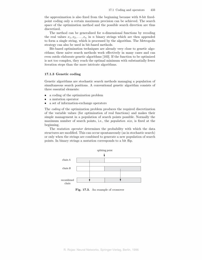
The mutation operator determines the probability with which the datastructures are modified. This can occur spontaneously (as in stochastic search)or only when the strings are combined to generate a new population of searchpoints. In binary strings a mutation corresponds to a bit flip.

chain A

chain B

recombinedchain

splitting point

Fig. 17.3. An example of crossover




The information exchange operators control the recombination of thesearch points in order to generate a new, better population of points at eachiteration step. Before recombining, the function to be optimized must be eval-uated for all data structures in the population. The search points are thensorted in the order of their function value, i.e., in the order of their so-calledfitness. In a minimization problem the points which are placed at the begin-ning of the list are those for which the function value is lowest. Those pointsfor which the function to be minimized has the greatest function value areplaced at the end of the list. Following this sorting operation the points arereproduced in such a way that the data structures at the beginning of the listare selected with a higher probability than the ones at the end of the list. Atypical reproduction operator is crossover. Two strings A and B are selectedas “parents” and a cut-off position for both is selected at random. The newstring is formed so that the left side comes from one parent and the rightside from the other. This produces an interchange of the information storedin each parent string. The whole process is reminiscent of genetic exchange inliving organisms. A favorable interchange can produce a string closer to theminimum of the target function than each parent string by itself. We expectthe collective fitness of the population to increase in time. The algorithm canbe stopped when the fitness of the best string in the population no longerchanges.

For a more precise illustration of genetic algorithms we will now considerthe problem of string coding.

Optimization problems whose variables can be coded in a string are suit-able for genetic algorithms. To this end an alphabet for the coding of theinformation must be agreed upon. Consider, for example, the following prob-lem: a keyboard is to be optimized by distributing the 26 letters A to Z over26 positions. The learning time of various selected candidates is to be mini-mized. This problem could only be solved by a multitude of experiments. Asuitable coding would be a string with 26 symbols, each of which can be oneof the 26 letters (without repeats). So the alphabet of the coding consists of26 symbols, and the search space of the problem contains 26! different combi-nations. For Asian languages the search space is even greater and the problemcorrespondingly more difficult [162].

A binary coding of the optimization problem is ideal because in this waythe mutation and information exchange operators are simple to implement.With neural networks, in which the parameters to be optimized are usuallyreal numbers, the definition of an adequate coding is an important problem.There are two alternatives: floating-point or fixed-point coding. Both possibil-ities can be used, whereby fixed-point coding allows more gradual mutationsthan floating-point coding [221]. With the latter the change of a single bit inthe exponent of the number can cause a dramatic jump. Fixed-point codingis usually sufficient for dealing with the parameters of neural networks (seeSect. 8.2.3).



17.2 Properties of genetic algorithms 435

17.1.4 Information exchange with genetic operators

Genetic operators determine the way new strings are generated out of existingones. The mutation operator is the simplest to describe. A new string canbe generated by copying an old string position by position. However, duringcopying each symbol in the string can be modified with a certain probability,the mutation rate. The new string is then not a perfect copy and can be usedas a new starting point for a search operation in the definition domain of thefunction to be optimized.

The crossover operator was described in the last section. With this oper-ator portions of the information contained in two strings can be combined.However an important question for crossover is at which exact places we areallowed to partition the strings.

Both types of operator can be visualized in the case of function optimiza-tion. Assume that the function x �→ x2 is to be optimized in the interval[0, 1]. The values of the variable x can be encoded with the binary fixed-pointcoding x = 0.b9b8b7b6b5b4b3b2b1b0. Thus there are 1024 different values of xand only one of them optimizes the proposed quadratic function. The codeused discretizes the definition space of the function. The minimum distancebetween consecutive values of x is 2−10.

A mutation of the i-th bit of the string 0.b9b8b7b6b5b4b3b2b1b0 producesa change of x of δ = 2−i. Thus a new point x + δ is generated. In this casethe mutation corresponds to a stochastic search operation with variable steplength.

When the number x = 0.b9b8b7b6b5b4b3b2b1b0 is recombined with the num-ber y = 0.a9a8a7a6a5a4a3a2a1a0, a cut-off position i is selected at random.The new string, which belongs to the number z, is then:

z = 0.b9b8 · · · biai−1 · · · a0.

The new point z can also be written as z = x + δ, where δ is dependent onthe bit sequences of x and y. Crossover can therefore be interpreted as a fur-ther variation of stochastic search. But note that in this extremely simplifiedexample any gradient descent method is much more efficient than a geneticalgorithm.

17.2 Properties of genetic algorithms

Genetic algorithms have made a real impact on all those problems in whichthere is not enough information to build a differentiable function or where theproblem has such a complex structure that the interplay of different parame-ters in the final cost function cannot be expressed analytically.




17.2.1 Convergence analysis

The advantages of genetic algorithms first become apparent when a populationof strings is observed. Let f be the function x �→ x2 which is to be maximized,as before, in the interval [0, 1]. A population of N numbers in the interval [0, 1]is generated in 10-bit fixed-point coding. The function f is evaluated for eachof the numbers x1, x2, . . . , xN , and the strings are then listed in descendingorder of their function values. Two strings from this list are always selectedto generate a new member of a new population, whereby the probability ofselection decreases monotonically in accordance with the ascending positionin the sorted list.

The computed list contains N strings which, for a sufficiently large N ,should look like this:

1 0.1∗∗∗∗∗∗∗∗∗∗1 0.1∗∗∗∗∗∗∗∗∗∗...

...1 0.0∗∗∗∗∗∗∗∗∗∗

The first positions in the list are occupied by strings in which the first bit afterthe point is a 1 (i.e., the corresponding numbers lie in the interval [0.5, 1]). Thelast positions are occupied by strings in which the first bit after the decimalpoint is a 0. The asterisk stands for any bit value from 0 to 1, and the zero infront of the point does not need to be coded in the strings. The upper stringsare more likely to be selected for a recombination, so that the offspring ismore likely to contain a 1 in the first bit than a 0. The new population isevaluated and a new fitness list is drawn up. On the other hand, strings witha 0 in the first bit are placed at the end of the list and are less likely to beselected than the strings which begin with a 1. After several generations nomore strings with a 0 in the first bit after the decimal point are contained inthe population.

The same process is repeated for the strings with a zero in the secondbit. They are also pushed towards extinction. Gradually the whole populationconverges to the optimal string 0.1111111111 (when no mutation is present).

With this quadratic function the search operation is carried out within avery well-ordered framework. New points are defined at each crossover, butsteps in the direction x = 1 are more likely than steps in the opposite direction.The step length is also reduced in each reproduction step in which the 0 bitsare eliminated from a position. When, for example, the whole population onlyconsists of strings with ones in the first nine positions, then the maximumstep length can only be 2−10.

The whole process strongly resembles simulated annealing. There, stochas-tic jumps are also generated, whereby transitions in the maximization direc-tion are more probable. In time the temperature constant decreases to zero,so that the jumps become increasingly smaller until the system freezes at alocal maximum.




John Holland [195] suggested the notion of schemata for the convergenceanalysis of genetic algorithms. Schemata are bit patterns which function asrepresentatives of a set of binary strings. We already used such bit patternsin the example above: the bit patterns can contain each of the three symbols0, 1 or ∗. The schema ∗∗00∗∗, for example, is a representative of all stringsof length 6 with two zeros in the central positions, such as: 100000, 110011,010010, etc.

During the course of a genetic algorithm the best bit patterns are graduallyselected, i.e., those patterns which minimize/maximize the value of the func-tion to be optimized. Normal genetic algorithms consist of a finite repetitionof the three steps:

1. selection of the parent strings,2. recombination,3. mutation.

This raises the question: how likely is it that the better bit patterns survivefrom one generation of a genetic algorithm to another? This depends on theprobability with which they are selected for the generation of new child stringsand with which they survive the recombination and mutation steps. We nowwant to calculate this probability.

In the algorithm to be analyzed, the population consists of a set of Nbinary strings of length � at time t. A string of length � which contains one ofthe three symbols 0, 1, or � in each position is a bit pattern or schema. Thesymbol � represents a 0 or a 1. The number of strings in the population ingeneration t which contain the bit pattern H is called o(H, t). The diameterof a bit pattern is defined as the length of the pattern’s shortest substringthat still contains all fixed bits in the pattern. For example, the bit pattern∗∗1∗1∗∗ has diameter three because the shortest fragment that contains bothconstant bits is the substring 1∗1 and its length is three. The diameter of a bitpattern H is called d(H), with d(H) ≥ 1. It is important to understand thata schema is of the same length as the strings that compose the population.

Let us assume that f has to be maximized. The function f is defined overall binary strings of length � and is called the fitness of the strings. Two parentstrings from the current population are always selected for the creation of anew string. The probability that a parent string Hj will be selected from Nstrings H1, H2, . . . , HN is

p(Hj) =f(Hj)∑Ni=1 f(Hi)

.

This means that strings with greater fitness are more likely to be selectedthan strings with lesser fitness. Let fμ be the average fitness of all strings inthe population, i.e.,

fμ =1N

N∑i=1

f(Hi).




The probability p(Hj) can be rewritten as

p(Hj) =f(Hj)Nfμ

.

The probability that a schema H will be passed on to a child string can becalculated in the following three steps:

i) Selection

Selection with replacement is used, i.e., the whole population is the basis foreach individual parent selection. It can occur that the same string is selectedtwice. The probability P that a string is selected which contains the bit patternH is:

P =f(H1)Nfμ

+f(H2)Nfμ

+ · · ·+ f(Hk)Nfμ

,

where H1, H2, . . . , Hk represent all strings of the generation which containthe bit pattern H . If there are no such strings, then P is zero.

The fitness f(H) of the bit pattern H in the generation t is defined as

f(H) =f(H1) + f(H2) + · · ·+ f(Hk)

o(H, t).

Thus P can be rewritten as

P =o(H, t)f(H)

Nfμ.

The probability PA that two strings which contain pattern H are selected asparent strings is given by

PA =(o(H, t)f(H)

Nfμ

)2

.

The probability PB that from two selected strings only one contains the pat-tern H is:

PB = 2o(H, t)f(H)

Nfμ

(1− o(H, t)f(H)

Nfμ

).

ii) Recombination

For the recombination of two strings a cut-off point is selected between thepositions 1 and �− 1 and then a crossover is carried out. The probability Wthat a schema H is transmitted to the new string depends on two cases. Ifboth parent strings contain H , then they pass on this substring to the newstring. If only one of the strings contains H , then the schema is inherited at




most half of the time. The substring H can also be destroyed with probability(d(H)− 1)/(�− 1) during crossover. This means that

W ≥(o(H, t)f(H)

Nfμ

)2

+22o(H, t)f(H)

Nfμ

(1− o(H, t)f(H)

Nfμ

)(1− d(H)− 1

�− 1

).

The probability W is greater than or equal to the term on the right in theabove inequality, because in some favorable cases the bit string is not destroyedby crossover (one parent string contains H and the other parent part of H).To simplify the discussion we will not examine all these possibilities. Theinequality for W can be further simplified to

W ≥ o(H, t)f(H)Nfμ

(1− d(H)− 1

�− 1

(1− o(H, t)f(H)

Nfμ

)).

iii) Mutation

When two strings are recombined, the information contained in them is copiedbit by bit to the child string. A mutation can produce a bit flip with the prob-ability p. This means that a schema H with b(H) fixed bits will be preservedafter copying with probability (1−p)b(H). If a mutation occurs the probabilityW of the schema H being passed on to a child string changes according toW ′, where

W ′ ≥ o(H, t)f(H)Nfμ

(1− d(H)− 1

�− 1

(1− o(H, t)f(H)

Nfμ

))(1 − p)b(H).

If in each generation N new strings are produced, the expected value of thenumber of strings which contain H in the generation t+ 1 is NW ′, that is

〈o(H, t+ 1)〉 ≥ o(H, t)f(H)fμ

(1− d(H)− 1

�− 1

(1− 0(H, t)f(H)

Nfμ

))(1− p)b(H).

(17.1)Equation (17.1) or slight variants thereof are known in the literature by thename “schema theorem” [195, 163]. This result is interpreted as stating thatin the long run the best bit patterns will diffuse to the whole population.

17.2.2 Deceptive problems

The schema theorem has to be taken with a grain of salt. There are somefunctions in which finding the optimal bit patterns can be extremely difficultfor a genetic algorithm. This happens in many cases when the optimal bits inthe selected coding exhibit some kind of correlation. Consider the followingfunction of n variables,

(x1, x2, . . . , xn) �→ x21 + · · ·+ x2

n

x21 + ε

+ · · ·+ x21 + · · ·+ x2

n

x2n + ε

,




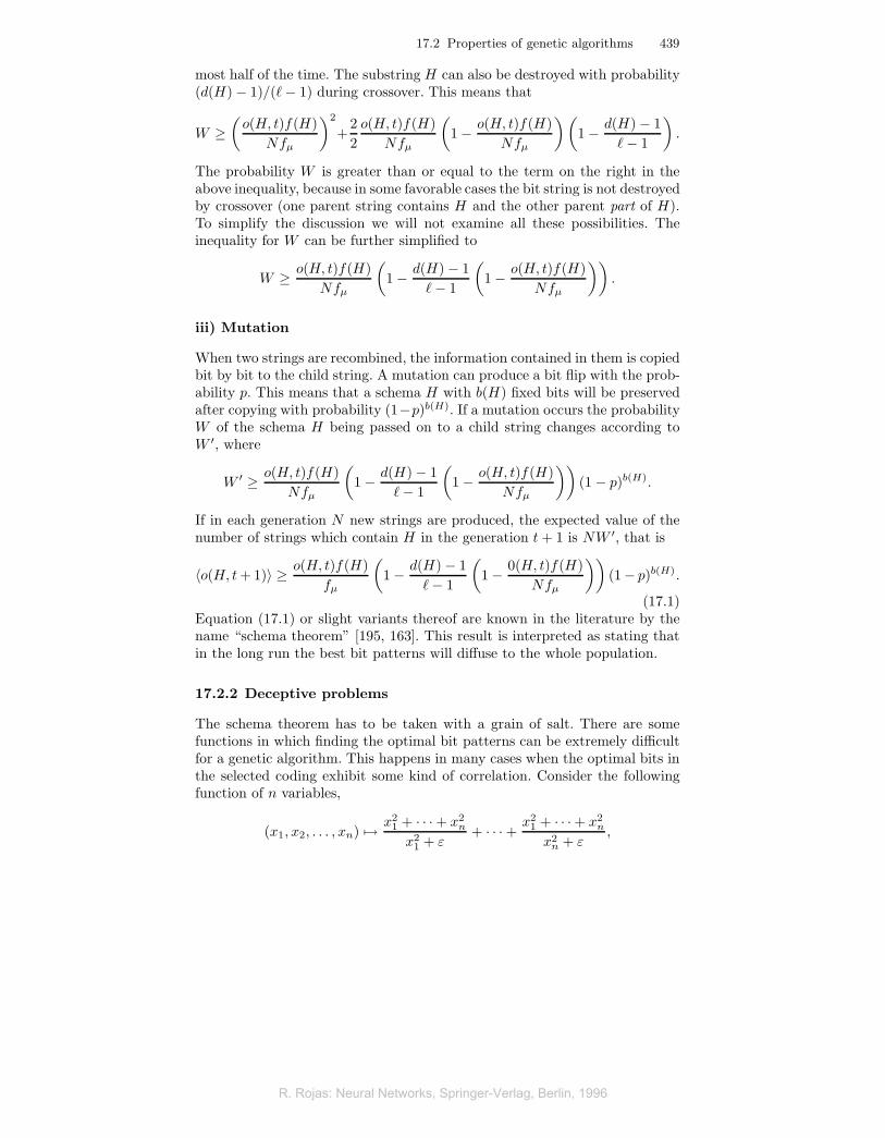
where ε is a small positive constant. The minimum of this function is locatedat the origin and any gradient descent method would find it immediately.However if the n parameters are coded in a single string using 10 bits, any timeone of these parameters approaches the value zero, the value of the functionincreases. It is not possible to approach the origin following the directionof the axes. This means that only correlated mutations of the n parametersare favorable, so that the origin is reached through the diagonal valleys ofthe fitness function. The probability of such coordinated mutations is verysmall when the number of parameters n and the number of bits used to codeeach parameter increases. Figure 17.4 shows the shape of the two-dimensionalversion of this problematic function.

010

2030

40

0

10

20

30

400

20

40

60

80

100

120

Fig. 17.4. A deceptive function

Functions which “hide” the optimum from genetic algorithms have beencalled deceptive functions by Goldberg and other authors. They mislead theGA into pursuing false leads to the optimum, which in many cases is onlyreached by pure luck.

There has been much research over the last few years on classifying thekinds of function which should be easy for a genetic algorithm to optimizeand those which should be hard to deal with. Holland and Mitchell defined so-called “royal road” functions [314], which are defined in such a way that severalparameters x1, x2, . . . , xn are coded contiguously and the fitness function f isjust a sum of n functions of each parameter, that is,

f(x1, x2, . . . , xn) = f1(x1) + f2(x2) + · · ·+ fn(xn).

When these functions are optimized, genetic algorithms rapidly find the nec-essary values for each parameter. Mutation and crossover are both beneficial.However, mere addition of a further function f ′ of the variables x1 and x2

can slow down convergence [141]. This happens because the additional termtends to select contiguous combinations of x1 and x2. If the contribution from




f ′(x1, x2) to the fitness function is more important than the contribution fromf3(x3), some garbage bits at the coding positions for x3 can become attachedto the strings with the optimum values for x1 and x2. They then get a “freeride” and become selected more often. That is why they are called hitch-hikingbits [142].

Some authors have argued in favor of the building block hypothesis to ex-plain why GAs do well in some circumstances. According to this hypothesisa GA finds building blocks which are then combined through the generationsin order to reach the optimal solution. But the phenomena we just pointedout, and the correlations between the optimization parameters, sometimespreclude altogether the formation of these building blocks. The hypothesishas received some strong criticism in recent years [166, 141].

17.2.3 Genetic drift

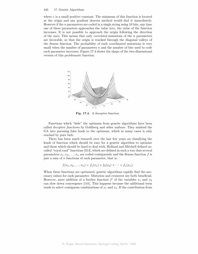
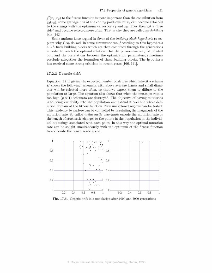
Equation (17.1) giving the expected number of strings which inherit a schemaH shows the following: schemata with above average fitness and small diam-eter will be selected more often, so that we expect them to diffuse to thepopulation at large. The equation also shows that when the mutation rate istoo high (p ≈ 1) schemata are destroyed. The objective of having mutationsis to bring variability into the population and extend it over the whole defi-nition domain of the fitness function. New unexplored regions can be tested.This tendency to explore can be controlled by regulating the magnitude of themutation rate. So-called metagenetic algorithms encode the mutation rate orthe length of stochastic changes to the points in the population in the individ-ual bit strings associated with each point. In this way the optimal mutationrate can be sought simultaneously with the optimum of the fitness functionto accelerate the convergence speed.

0.2 0.4 0.6 0.8 10

0.2

0.4

0.6

0.8

1

0.2 0.4 0.6 0.8 10

0.2

0.4

0.6

0.8

1

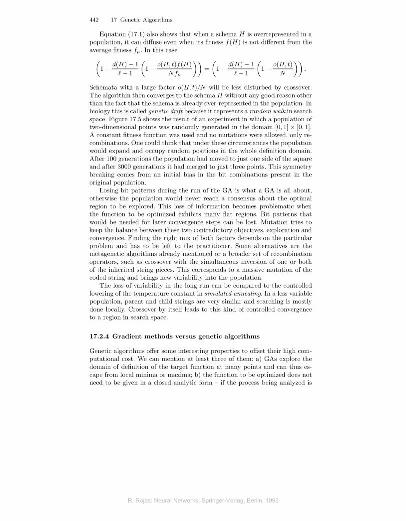
Fig. 17.5. Genetic drift in a population after 1000 and 3000 generations




Equation (17.1) also shows that when a schema H is overrepresented in apopulation, it can diffuse even when its fitness f(H) is not different from theaverage fitness fμ. In this case(

1− d(H)− 1�− 1

(1− o(H, t)f(H)

Nfμ

))=(

1− d(H)− 1�− 1

(1− o(H, t)

N

)).

Schemata with a large factor o(H, t)/N will be less disturbed by crossover.The algorithm then converges to the schema H without any good reason otherthan the fact that the schema is already over-represented in the population. Inbiology this is called genetic drift because it represents a random walk in searchspace. Figure 17.5 shows the result of an experiment in which a population oftwo-dimensional points was randomly generated in the domain [0, 1] × [0, 1].A constant fitness function was used and no mutations were allowed, only re-combinations. One could think that under these circumstances the populationwould expand and occupy random positions in the whole definition domain.After 100 generations the population had moved to just one side of the squareand after 3000 generations it had merged to just three points. This symmetrybreaking comes from an initial bias in the bit combinations present in theoriginal population.

Losing bit patterns during the run of the GA is what a GA is all about,otherwise the population would never reach a consensus about the optimalregion to be explored. This loss of information becomes problematic whenthe function to be optimized exhibits many flat regions. Bit patterns thatwould be needed for later convergence steps can be lost. Mutation tries tokeep the balance between these two contradictory objectives, exploration andconvergence. Finding the right mix of both factors depends on the particularproblem and has to be left to the practitioner. Some alternatives are themetagenetic algorithms already mentioned or a broader set of recombinationoperators, such as crossover with the simultaneous inversion of one or bothof the inherited string pieces. This corresponds to a massive mutation of thecoded string and brings new variability into the population.

The loss of variability in the long run can be compared to the controlledlowering of the temperature constant in simulated annealing. In a less variablepopulation, parent and child strings are very similar and searching is mostlydone locally. Crossover by itself leads to this kind of controlled convergenceto a region in search space.

17.2.4 Gradient methods versus genetic algorithms

Genetic algorithms offer some interesting properties to offset their high com-putational cost. We can mention at least three of them: a) GAs explore thedomain of definition of the target function at many points and can thus es-cape from local minima or maxima; b) the function to be optimized does notneed to be given in a closed analytic form – if the process being analyzed is



17.3 Neural networks and genetic algorithms 443

too complex to describe in formulas, the elements of the population are usedto run some experiments (numerical or in the laboratory) and the results areinterpreted as their fitness; c) since evaluation of the target function is inde-pendent for each element of the population, the parallelization of the GA isquite straightforward. A population can be distributed on several processorsand the selection process carried out in parallel. The kinds of recombinationoperator define the type of communication needed between the processors.

Straightforward parallelization and the possibility of their application inill-defined problems makes GAs attractive. De Jong has emphasized that GAsare not function optimizers of the kind studied in numerical analysis [105].Otherwise their range of applicability would be very narrow. As we alreadymentioned, in many cases a naive hill-climber is able to outperform complexgenetic algorithms. The hill-climber is started n times at n different positionsand the best solution is selected. A combination of a GA and hill-climbingis also straightforward: the elements in the population are selected in “Dar-winian” fashion from generation to generation, but can become better bymodifying their parameters in “Lamarckian” way, that is, by performing somehill-climbing steps before recombining. Davis [103] showed that many popularfunctions used as benchmarks for genetic algorithms can be optimized with asimple bit climber (stochastic bit-flipping). In six out of seven test functionsthe bit climber outperformed two variants of a genetic algorithm. It was threetimes faster than an efficient GA and twenty-three times faster than an ineffi-cient version. Ackley [8, 9] arrived at similar results when he compared sevendifferent optimization methods. Depending on the test function one or theother minimization strategies emerged victorious. These results only confirmwhat numerical analysts have known for a long time: there is no optimal op-timization method, it all depends on the problem at hand. Even if this is so,the attractiveness of easy parallelization is not diminished. If no best methodexists, we can at least parallelize those we have.

17.3 Neural networks and genetic algorithms

Our interest in genetic algorithms for neural networks has two sources: is itpossible to use this kind of approach to find the weights in a network? Andeven more important: is it possible to let networks evolve so that they find anoptimal topology? The question of network topology is one of those problemsfor which no closed-form fitness function over all possible configurations canbe given. We just propose a topology and let the network run, change thetopology again and look at the results. Before going into the details we have tolook at some specific characteristics of neural networks which seem to precludethe use of genetic algorithms.




17.3.1 The problem of symmetries

Before genetic algorithms can be used to minimize the error function of neu-ral networks, an appropriate code must be designed. Usually the weightsof the network are floating-point numbers. Assume that the m weightsw1, w2, . . . , wm have been coded and arranged in a string. The target functionfor the GA is the error of the network for a given training set. The code foreach parameter could consist of 20 bits, and in that case all network param-eters could be represented by a string of 20m bits. These strings are thenprocessed in the usual way.

1

0

-1

2

1

21

0

2

-12

1

0

1

0

0

1

0

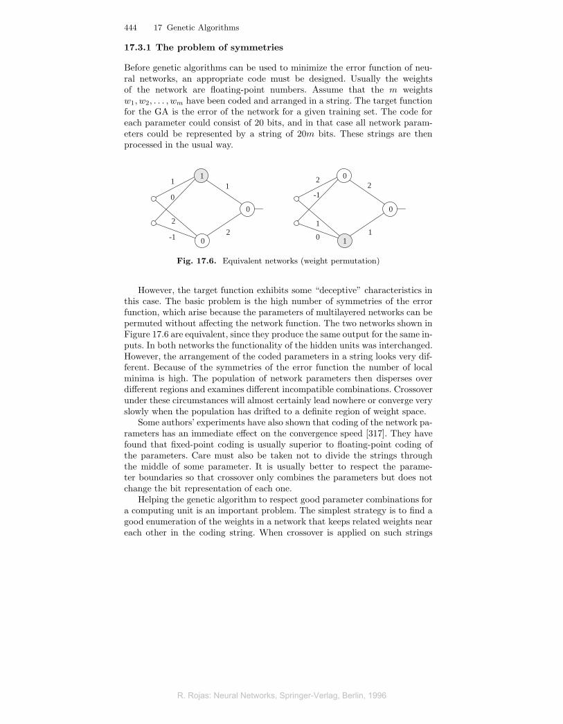
Fig. 17.6. Equivalent networks (weight permutation)

However, the target function exhibits some “deceptive” characteristics inthis case. The basic problem is the high number of symmetries of the errorfunction, which arise because the parameters of multilayered networks can bepermuted without affecting the network function. The two networks shown inFigure 17.6 are equivalent, since they produce the same output for the same in-puts. In both networks the functionality of the hidden units was interchanged.However, the arrangement of the coded parameters in a string looks very dif-ferent. Because of the symmetries of the error function the number of localminima is high. The population of network parameters then disperses overdifferent regions and examines different incompatible combinations. Crossoverunder these circumstances will almost certainly lead nowhere or converge veryslowly when the population has drifted to a definite region of weight space.

Some authors’ experiments have also shown that coding of the network pa-rameters has an immediate effect on the convergence speed [317]. They havefound that fixed-point coding is usually superior to floating-point coding ofthe parameters. Care must also be taken not to divide the strings throughthe middle of some parameter. It is usually better to respect the parame-ter boundaries so that crossover only combines the parameters but does notchange the bit representation of each one.

Helping the genetic algorithm to respect good parameter combinations fora computing unit is an important problem. The simplest strategy is to find agood enumeration of the weights in a network that keeps related weights neareach other in the coding string. When crossover is applied on such strings




α

α

α

α

α

α

α

α

α

1

2

3

4

5 6

7

8

9

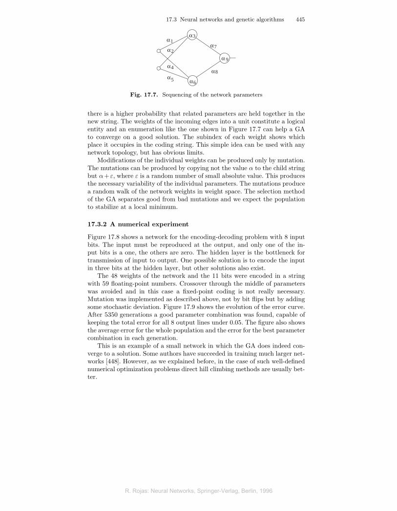
Fig. 17.7. Sequencing of the network parameters

there is a higher probability that related parameters are held together in thenew string. The weights of the incoming edges into a unit constitute a logicalentity and an enumeration like the one shown in Figure 17.7 can help a GAto converge on a good solution. The subindex of each weight shows whichplace it occupies in the coding string. This simple idea can be used with anynetwork topology, but has obvious limits.

Modifications of the individual weights can be produced only by mutation.The mutations can be produced by copying not the value α to the child stringbut α+ε, where ε is a random number of small absolute value. This producesthe necessary variability of the individual parameters. The mutations producea random walk of the network weights in weight space. The selection methodof the GA separates good from bad mutations and we expect the populationto stabilize at a local minimum.

17.3.2 A numerical experiment

Figure 17.8 shows a network for the encoding-decoding problem with 8 inputbits. The input must be reproduced at the output, and only one of the in-put bits is a one, the others are zero. The hidden layer is the bottleneck fortransmission of input to output. One possible solution is to encode the inputin three bits at the hidden layer, but other solutions also exist.

The 48 weights of the network and the 11 bits were encoded in a stringwith 59 floating-point numbers. Crossover through the middle of parameterswas avoided and in this case a fixed-point coding is not really necessary.Mutation was implemented as described above, not by bit flips but by addingsome stochastic deviation. Figure 17.9 shows the evolution of the error curve.After 5350 generations a good parameter combination was found, capable ofkeeping the total error for all 8 output lines under 0.05. The figure also showsthe average error for the whole population and the error for the best parametercombination in each generation.

This is an example of a small network in which the GA does indeed con-verge to a solution. Some authors have succeeded in training much larger net-works [448]. However, as we explained before, in the case of such well-definednumerical optimization problems direct hill climbing methods are usually bet-ter.




x1

x

x

x

x

x

x

x

2

3

5

6

7

8

4

Fig. 17.8. An 8-bit encoder-decoder

0

1

2

3

4

5

6

7

8

500 1500 2500 3500 4500

error

generations

5350

average error

best network

Fig. 17.9. Error function at each generation: population average and best network

Braun has shown how to optimize the network topology using geneticalgorithms [69]. He introduces order into the network by defining a fitnessfunction f made of several parts: one proportional to the approximation er-ror, and another proportional to the length of the network edges. The nodesare all fixed in a two-dimensional plane and the network is organized in lay-ers. The fitness function is minimized using a genetic algorithm. Edges withsmall weights are dropped stochastically. Smaller networks are favored in thecourse of evolution. The two-dimensional mapping is introduced to avoid de-




stroying good solutions when reproducing the population, as happens whenthe network symmetries are not considered.

17.3.3 Other applications of GAs

One field in which GAs seem to be a very appropriate search method is gametheory. In a typical mathematical game some rules are defined and the rewardfor the players after each move is given by a certain pay-off function. Math-ematicians then ask what is the optimal strategy, that is, how can a playermaximize his pay-off. In many cases the cumulative effect of the pay-off func-tion cannot be expressed analytically and the only possibility is to actuallyplay the game and compare the results using different strategies. An unknownfunction must be optimized and this is done with a computer simulation. Sincethe range of possible strategies is so large only a few variants are tested.

This is where GAs take over. A population of “players” is generated anda tournament is held. The strategy of each player must be coded in a datastructure that can be recombined and mutated. Each round of the tourna-ment is used to compute the pay-off for each strategy and the best playersprovide more genes for the next generation. Axelrod [36] did exactly this forthe problem known as the prisoner’s dilemma. In this game between two play-ers, each one decides independently whether he wants to cooperate with theother player or betray him. There are four possibilities each time: a) both play-ers cooperate; b) the first cooperates, the second betrays; c) the first betrays,the second cooperates; and c) both players betray each other. The pay-off foreach of the four combinations is shown in Figure 17.10. The letters C and Bstand for “cooperation” and “betrayal” respectively.

C D

C

D

first player

secondplayer

3

3

0

5

5

0

1

1

Fig. 17.10. Pay-off matrix for the prisoner’s dilemma

The pay-off matrix shows that there is an incentive to commit treachery.The pay-off when one of the players betrays the other, who wants to cooperate,is 5. Moreover, the betrayed player does not get any pay-off at all. But if both




players betray, the pay-off for both is just 1 point. If both players cooperateeach one gets 3 points.

If the game is played only once, the optimal strategy is betraying. Fromthe viewpoint of each player the situation is the following: if the other playercooperates, then the pay-off can be maximized by betraying. And if the otherplayer betrays, then at least one point can be saved by committing treacherytoo. Since both viewpoints are symmetrical, both players betray.

However, the game becomes more complicated if it is repeated an indefinitenumber of times in a tournament. Two players willing to cooperate can reaplarger profits than two players betraying each other. In that case the playersmust keep a record of the results of previous games with the same partnerin order to adapt to cooperative or uncooperative adversaries. Axelrod andHamilton [35] held such a tournament in which a population of players oper-ated with different strategies for the iterated prisoner’s dilemma. Each playercould store only the results of the last three games against each opponent andthe players were paired randomly at each iteration of the tournament. It wassurprising that the simplest strategy submitted for the tournament collectedthe most points. Axelrod called it “tit for tat” (TFT) and it consists in justrepeating the last move of the opponent. If the adversary cooperated the lasttime, cooperation ensues. If the adversary betrayed, he is now betrayed. Twoplayers who happen to repeat some rounds of cooperation are better off thanthose that keep betraying. The TFT strategy is initialized by offering coop-eration to a yet unknown player, but responds afterwards with vengeance foreach betrayal. It can thus be exploited no more than once in a tournament.

For the first tournament, the strategies were submitted by game theo-rists. In a second experiment the strategies were generated in the computerby evolving them over time [36]. Since for each move there are four possibleoutcomes of the game and only the last three moves were stored, there are64 possible recent histories of the game against each opponent. The strategyof each player can be coded simply as a binary vector of length 64. Eachcomponent represents one of the possible histories and the value 1 is inter-preted as cooperation in the next move, whereas 0 is interpreted as betrayal.A vector of 64 ones, for example, is the coding for a strategy which always co-operates regardless of the previous game history against the opponent. Aftersome generations of a tournament held under controlled conditions and withsome handcrafted strategies present, TFT emerged again as one of the beststrategies. Other strategies with a tendency to cooperate also evolved.

17.4 Historical and bibliographical remarks

At the end of the 1950s and the beginning of the 1960s several authors indepen-dently proposed the use of evolutionary methods for the solution of optimiza-tion problems. Goldberg summarized this development from the American



17.4 Historical and bibliographical remarks 449

perspective [163]. Fraser, for example, studied the optimization of polynomi-als, borrowing his methods from genetics. Other researchers applied GAs inthe 1960s to the solution of such diverse problems as simulation, game theory,or pattern recognition. Fogel and his coauthors studied the problems of mu-tating populations of finite state automata and recombination, although theystopped short of using the crossover operator [139].

John Holland was the first to try to examine the dynamic of GAs andto formulate a theory of their properties [195]. His book on the subject is aclassic to this day. He proposed the concept of schemata and applied statisticalmethods to the study of their diffusion dynamics. The University of Michiganbecame one of the leading centers in this field through his work.

In other countries the same ideas were taking shape. In the 1960s Rechen-berg [358] and Schwefel [394] proposed their own version of evolutionary com-putation, which they called evolution strategies. Some of the problems thatwere solved in this early phase were, for example, hard hydrodynamic opti-mization tasks, such as finding the optimal shape of a rocket booster. Schwefelexperimented with the evolution of the parameters of the genetic operators,maybe the first instance of metagenetic algorithms [37]. In the 1980s Rechen-berg’s lab in Berlin solved many other problems such as the optimal profileof wind concentrators and airplane wings.

Koza and Rice showed that it is possible to optimize the topology of neuralnetworks [260]. Their methods make use of the techniques developed by Kozato breed Lisp programs, represented as trees of terms. Crossover exchangeswhole branches of two trees in this kind of representation. Belew and coau-thors [51] examined the possibility of applying evolutionary computation toconnectionist learning problems.

There has been much discussion recently on the merits of genetic algo-rithms for static function optimization [105]. Simple minded hill-climbing al-gorithms seem to outperform GAs when the function to be optimized is fixed.Baluja showed in fact that for a large set of optimization problems GAs donot offer a definitive advantage when compared to other optimization heuris-tics, either in terms of total function evaluations or in quality of the solutions[40]. More work must be still done to determine under which situations (dy-namic enviroments, for example) GAs offer a definitive advantage over otheroptimization methods.

The prisoner’s dilemma was proposed by game-theoreticians in the 1950sand led immediately to many psychological experiments and mathematicalarguments [350]. The research of Axelrod on the iterated prisoner’s dilemmacan be considered one of the milestones in evolutionary computation, since itopened this whole field to the social scientists and behavior biologists, whoby the nature of their subject had not transcended the level of qualitativedescriptions [104, 453]. The moral dilemma of the contradiction between al-truism and egoism could now be modeled in a quantitative way, althoughAxelrod’s results have not remained uncontested.




Exercises

1. How does the schema theorem (17.1) change when a crossover probabilitypc is introduced? This means that with probability pc, crossover is usedto combine two strings, otherwise one of the parent strings is copied.

2. Train a neural network with a genetic algorithm. Let the number ofweights increase and observe the running time.

3. Propose a coding method for a metagenetic algorithm that lets the mu-tation rate and the crossover probability evolve.

4. The prisoner’s dilemma can be implemented on a cellular automaton. Theplayers occupy one square of a two-dimensional grid and interact with theirclosest neighbors. Simulate this game in the computer and let the systemevolve different strategies.



Documents

17 Genetic Algorithmspage.mi.fu-berlin.de/rojas/neural/chapter/K17.pdf17 Genetic Algorithms 17.1 Coding and operators Learning in neural networks is an optimization process by which