18-819F: Introduction to Quantum Computing 47-779/47-785

18-819F: Introduction to Quantum Computing 47-779/47-785: Quantum Integer Programming

& Quantum Machine Learning

Mathematical Programming

Lecture 03

2021.09.09

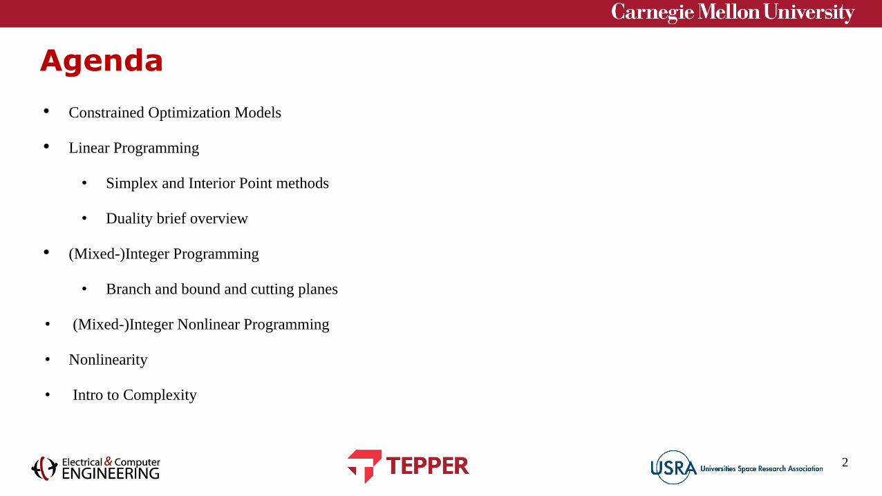
• Constrained Optimization Models

• Linear Programming

• Simplex and Interior Point methods

• Duality brief overview

• (Mixed-)Integer Programming

• Branch and bound and cutting planes

• (Mixed-)Integer Nonlinear Programming

• Nonlinearity

• Intro to Complexity

2

Agenda

● Exploration of real-world, looking for optimal solution can be time-consuming, expensive and prone to

errors

● Instead, we would like to have a model of the real-world

○ Represent our understanding of the real world

○ Incorporate assumptions and simplifications

○ Tradeoff between tractable and valid

● A useful paradigm is Mathematical Programming, where we write in mathematical equations

○ Objective(s)

○ Constraint(s)

■ All with respect to certain variables

3

Constrained Optimization Models

● Define the problem

● Formulate the model

○ Requirements

○ Simplifications

○ Assumptions

● Solve / Analyze the model

● Interpret the results

• All steps are vital to provide a solution!

4

Operations Research approach

Let’s propose a production plan that increases the profit of a company!

… we need more data than that.

The company only produces a finite set of products and each has its price. Besides, there are some production

limitations.

To propose a model of this situation we need to identify certain key aspects of the problem.

● What are relevant parameters or data?

● Which decisions can we make? What is unknown? What is controllable?

● What limitations are relevant? What determines how a solution is valid (feasibility)?

● What is our goal?

Once those are clear, we can propose a model.

5

Simple example

After addressing those questions we reach the following problem statement.

Suppose there is a company that produces two different product, A and B, which can be sold at different values, $5.5 and

$2.1 per unit, respectively.

The company only counts with a single machine with electricity usage of at most 17kW/day; and producing each A and B

consumes 8kW/day and 2kW/day, respectively.

Besides, the company can only produce at most 2 more units of A than B per day.

This is a valid model, but it would be easier to solve if we had a mathematical representation.

Assuming the units produced of A are and of B are we have

6

Simple example

[1] Adapted from Integer Programming (1st ed. 2014) by

Michele Conforti, Gérard Cornuéjols, and Giacomo Zambelli

7

A simplification of the general model presented

before assumes that all the constraints and objective

are linear, and the variables are continuous

The feasible region of a Linear Program (LP) is a

convex polyhedron Interior-point methods

● Path through interior of polytope

● Polynomial time

Simplex methods

● Vertex hopping

● (Worst-case) Exponential time

Most solvers use simplex!

● 1e7 variables is tractable!

Linear Programming



8

1. Write the “simplex tableau”

2. Convert to canonical form (select basis)

3. “Price out” basic variables

4. If solution can be improved, we pivot (swap

basic and non-basic variables)

Can efficiently restart from any feasible solution

Simplex (overview)



Basic variablesNon-basic variables

(assumed=0

Basic variables

values

Objective valueRelative costs

Modeling and Simplex method

9

Linear Programming

Let’s jump to the code!

https://colab.research.google.com/github/bernalde/QuIPML/blob/main/notebooks/Noteboo

k%201%20-%20LP%20and%20IP.ipynb

https://colab.research.google.com/github/bernalde/QuIPML/blob/main/notebooks/Notebook%201%20-%20LP%20and%20IP.ipynb

10

● More details to it but the basics

● Intuition: starting from a feasible point, we

approach the edges by having a monotonic

barrier when close.

● Synonyms: Barrier method

● Not very efficient at restart

● Very useful when problems are dual

degenerate

● What is duality?

Interior-point (brief overview)

[1] Adapted from Integer Programming (1st ed. 2014) by Michele Conforti, Gérard Cornuéjols, and Giacomo Zambelli

[2] https://en.wikipedia.org/wiki/Karmarkar%27s_algorithm

Interior point method

11

Linear Programming

Back to the code!




12

The Lagrangian function (with deep meaning

in classical mechanics and the least energy

principle) defines a lower bound on our

optimization problem, so we maximize itFor LPs (and in general convex problems) the

following holds:

Duality (very brief overview)



Lagrangian or dual multipliers

Simplex LP solvers Barrier LP Solvers

13

LP – State of the art

[1] http://plato.asu.edu/bench.html

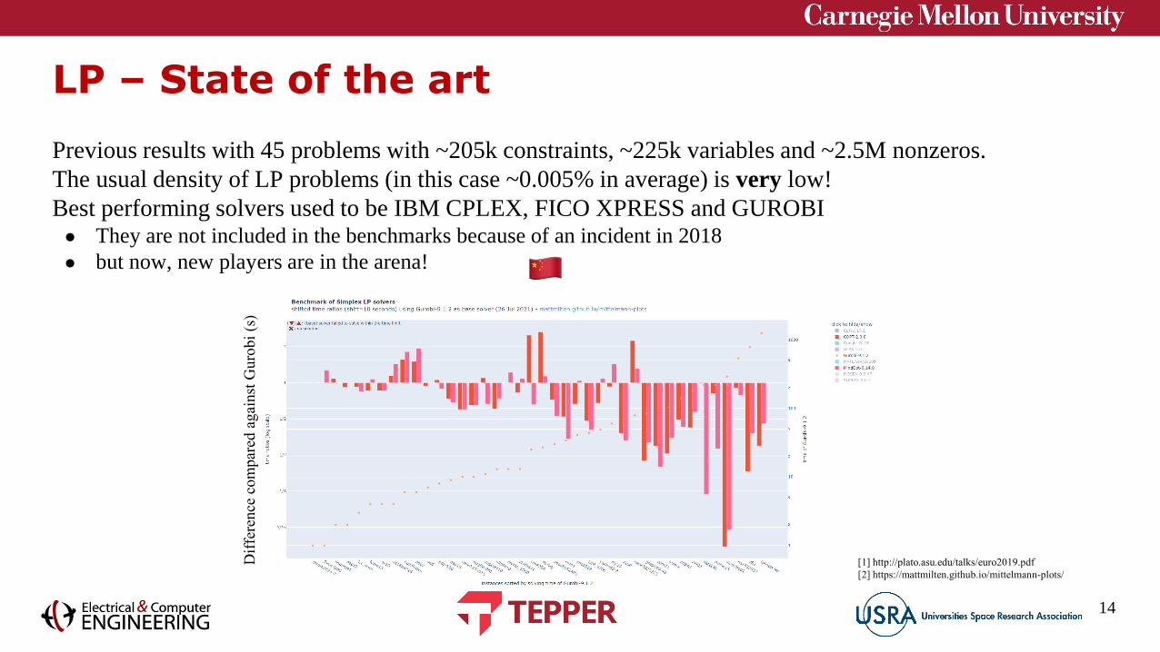
Previous results with 45 problems with ~205k constraints, ~225k variables and ~2.5M nonzeros.

The usual density of LP problems (in this case ~0.005% in average) is very low!

Best performing solvers used to be IBM CPLEX, FICO XPRESS and GUROBI ● They are not included in the benchmarks because of an incident in 2018

● but now, new players are in the arena!

14

LP – State of the art

Dif

fere

nce

com

par

ed a

gai

nst

Guro

bi

(s)

[1] http://plato.asu.edu/talks/euro2019.pdf

[2] https://mattmilten.github.io/mittelmann-plots/

15

Simple example - Continued

We found that the optimal solution was to produce 3.3 units of B, 1.3 units of A, and that would yield a

profit of $14.08.

But what if we can only produce an integer number of products?

We modify our formulation to include this new information.

The feasible region is no longer convex![1] Adapted from Integer Programming (1st ed. 2014) by Michele Conforti, Gérard Cornuéjols, and Giacomo Zambelli

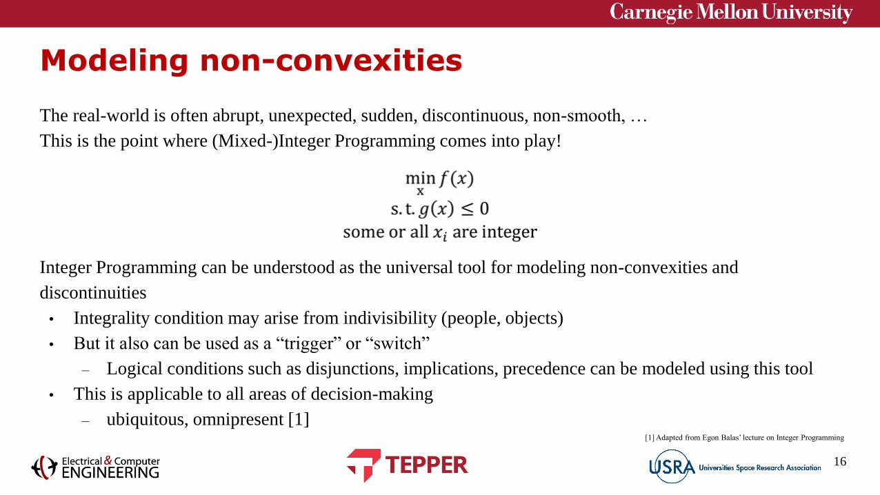
The real-world is often abrupt, unexpected, sudden, discontinuous, non-smooth, …

This is the point where (Mixed-)Integer Programming comes into play!

Integer Programming can be understood as the universal tool for modeling non-convexities and

discontinuities

• Integrality condition may arise from indivisibility (people, objects)

• But it also can be used as a “trigger” or “switch”

– Logical conditions such as disjunctions, implications, precedence can be modeled using this tool

• This is applicable to all areas of decision-making

– ubiquitous, omnipresent [1]

16

Modeling non-convexities

[1] Adapted from Egon Balas’ lecture on Integer Programming

How hard can it be just to look at all the possible values, checking if they satisfy the constraints (being

feasible) and comparing their objective function?

● Assuming only binary variables, the number of solutions grows as

● Many problems actually deal with permutations (assignments) therefore the number of solutions grow as

17

Enumerating

[1] Integer Programming (1st ed. 2014) by Michele Conforti, Gérard Cornuéjols, and Giacomo Zambelli

Solution and Enumeration

18

(Mixed-)Integer Programming

Back to the code!




19

A Mixed-Integer Program (MIP) is an optimization

problem of the form

Main concern is that is a strongly NP-complete

problem

Branch-and-bound

• Solution of each search node using linear

programming

Cutting plane methods

• Polyhedral theory

Enhanced with constraint programming methods

• Logic inference

• Domain reduction


[1] https://www.ferc.gov/CalendarFiles/20100609110044-Bixby,%20Gurobi%20Optimization.pdf

[2] R. Kannan and C. L. Monma, On the computational complexity of integer programming problems, vol. 157, Springer-Verlag, 1978, pp. 161–172.

[3] https://www.slideshare.net/IBMOptimization/2013-11-informs12yearsofprogress

20

Branch-and-boundCutting-plane methods


[1] Integer Programming (1st ed. 2014) by Michele Conforti, Gérard Cornuéjols, and Giacomo Zambelli

•Speedup between CPLEX 1.2 (1991) and CPLEX 11 (2007): 29,000

times

•Gurobi 1.0 (2009) comparable to CPLEX 11

•Speedup between Gurobi 1.0 and Gurobi 8.0 (2018): 91 times

•Total speedup 1991-2018: 2’600,000 times

21


•A MIP that would have taken 30 days to solve 27 years ago can now be solved in the same 25-year-old

computer in less than one second

•Hardware speed: 122.3 Pflops/s in 2018 vs. 59.7 Gflops/s in 1993 2’000,000 times

•Total speedup: 5.4 trillion times!

•A MIP that would have taken 171,000 years to solve 27 years ago can now be solved in a modern

computer in less than one second[1] https://www.ferc.gov/CalendarFiles/20100609110044-Bixby,%20Gurobi%20Optimization.pdf

[2] https://www.slideshare.net/IBMOptimization/2013-11-informs12yearsofprogress

22

Where is the improvement coming from?


[1] Integer Programming (1st ed. 2014) by Michele Conforti,

Gérard Cornuéjols, and Giacomo Zambelli

23

Benchmark coming from MIPlib 2017, a 1065

collection of challenging MIPs that ranging from 1

to 19M of constraints and from 3 to 38M of

variables.

Best commercial solvers are currently IBM CPLEX,

FICO XPRESS and GUROBI.

● Focus on parallelization has been a center of

research with many open questions there (usage

of GPUs is not trivial for these algorithms)

(M)IP State of the art

The real-world is apart of abrupt, nonlinear!

Although we can model discontinuities with integer variables, we can summarize more information using

nonlinear constraints and objectives

• Assumption that does not hold in general

• This only makes our problem harder

24

Modeling the real-world

[1] https://www.vox.com/2018/4/28/17292244/flat-earthers-

explain-philosophy

25

So far, we have only discussed linear constraints and

objective(s), but nonlinearity is key to modeling.

(Mixed-)Integer Nonlinear Programming

[1] COSC 545 - Theory of Computation, Georgetown University. Retrieved from

http://people.cs.georgetown.edu/~cnewport/teaching/cosc545-spring14/ on 02/17/2019.

Branch-and-bound methods (M)I Linear Programming based methods

26

(Mixed-)Integer Nonlinear Programming

Actual BB Tree after 360s w/o preprocessing (~100k nodes)

Underestimate of

objective function

Overestimate of the

feasible region

[1] Belotti, P., Kirches, C., Leyffer, S., S., Linderoth, J., Luedtke,

J., and Mahajan, A. “Mixed-integer nonlinear optimization” 2012

27

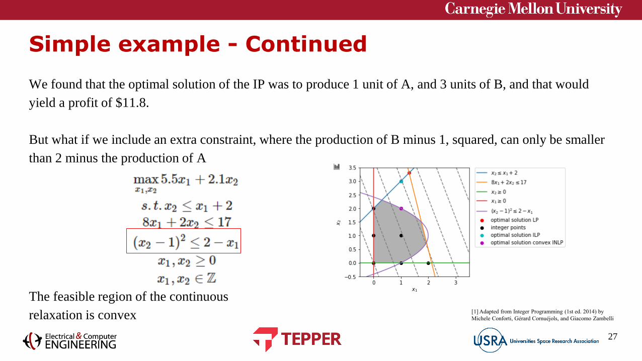
Simple example - Continued

We found that the optimal solution of the IP was to produce 1 unit of A, and 3 units of B, and that would

yield a profit of $11.8.

But what if we include an extra constraint, where the production of B minus 1, squared, can only be smaller

than 2 minus the production of A

The feasible region of the continuous

relaxation is convex [1] Adapted from Integer Programming (1st ed. 2014) by


Solution

28

Convex (Mixed-)Integer Nonlinear Programming

Back to the code!




Branch-and-bound methods (M)ILP based methods

29

Convex (M)INLP State of the art

Complexity boundary does not lie between linearity and nonlinearity

But between convexity and non-convexity.

Convex (M)INLP problems are more challenging but manageable

Benchmark from 335 problems with ~1000 variables and constraints in average

[1] Kronqvist, J., Bernal, D. E., Lundell, A. and Grossmann, I. E. [2018], `A review and comparison of solvers

for convex MINLP', Optimization and Engineering pp. 1-59.

We found that the optimal solution of the convex INLP was to produce 1 unit of A, and 2 units of B, and that

would yield a profit of $9.7.

Finally, we include an extra constraint, where the production of B minus 1, squared, can only be greater than

1/2 plus the production of A

The feasible region of the continuous

relaxation is convex!!!

30

Simple example – Final version

[1] Adapted from Integer Programming (1st ed. 2014) by Michele Conforti, Gérard Cornuéjols, and Giacomo Zambelli

Solution

31

Non-Convex (Mixed-)Integer Nonlinear Programming

Back to the code!




32

Benchmark coming from MINLPLib with instances

with ~2500 variables and constraints.

BARON is the most performant solver with a

geometric mean time to solve these instances of

~300 seconds.

Classical (M)IP solvers are increasing their

capabilities to deal with nonlinearities

Nonconvex (M)NLIP State of the art

● IBM CPLEX can solve problems with convex quadratic constraints

● FICO XPRESS can solve nonlinear programs through linearization

● GUROBI can solve non-convex quadratic and bilinear programs

c

[1] http://plato.asu.edu/bench.html

[2] http://minlplib.org

When analyzing an algorithm, we are interested in the amount of time and memory that it will take to solve it.

• To be safe this is usually answered in the worst-case scenario

• The discussion here will be mainly the time complexity of algorithms.

• We will use the “big-O” notation when given two functions , , where is an

unbounded subset of we write that if there exists a positive real number and such that

for every then

• For us is going to be the set of instances or problems, and an algorithm is a procedure that will give a

correct answer is a finite amount of time.

• An algorithm solves a problem in polynomial time if the function that measures its arithmetic operations

is polynomially bounded by the function encoding the size of the problem

33

Complexity introduction



● If there exists an algorithm that solves a problem in polynomial time, then that problem belongs to the complexity

class P

○ For example LP belongs to P because the interior point algorithm solves it in poly-time

● A decision problem is one with answer “yes” or “no”

● The complexity class NP, non-deterministic polynomial, is the class of all decision problems where the “yes”-

answer can be verified in poly-time

● If all the decision problems in NP can be reduced in poly-time to a problem Q, then Q is said to be NP-complete

○ “Is a (mixed-)integer linear set empty?” belongs to NP and is actually NP-complete

34


[1] Adapted from Integer Programming (1st ed. 2014) by Michele Conforti,


[2] Cook, Stephen A, The Complexity of Theorem-Proving Procedures (1971)

● A problem Q can be called NP-hard if all problems in NP can be reduced to Q in poly-time

○ Integer Programming is NP-hard

■ Since we can transform any NP problem into an integer program in poly-time, if there exists an algorithm

to solve IP in poly-time, then we can solve any NP problem in poly-time: P=NP

● Integer programs with quadratic constraints are proved to be undecidable

○ Even after a long time without finding a solution, we cannot conclude none exists…

○ MINLP are tough!

35


[1] Adapted from Integer Programming (1st ed. 2014) by Michele Conforti,


[2] Cook, Stephen A, The Complexity of Theorem-Proving Procedures (1971)

● A problem is said to belong to the complexity class BPP, bounded-error probabilistic polynomial time, if there is an

algorithm that solves it such that

○ It is allowed to flip coins and make random decisions

○ It is guaranteed to run in polynomial time

○ On any given run of the algorithm, it has a probability of at most 1/3 of giving the wrong answer, whether the

answer is YES or NO.

36


● There exists another complexity class called BQP,

bounded-error quantum polynomial time, which is the

quantum analogue of BPP

○ We hope that some problems belong to BQP and

not to BPP to observe Quantum Advantage

■ E.g., Integer factorizationThe suspected relationship of BQP to other problem spaces

[1] Michael Nielsen and Isaac Chuang (2000). Quantum Computation and Quantum

Information. Cambridge: Cambridge University Press. ISBN 0-521-63503-9.

Integer Programs lie at a very special intersection since they are:

• Interesting from an academic point of view

• Useful from a practical point of view

• Challenging from a computational point of view

We do not expect to observe Quantum Advantage by solving Integer Programs using Quantum Computers

(but who knows right? Maybe P=BPP=BQP=NP)

We are still dealing with complicated problems that require answers, so we are going to try our best to solve

them.

Welcome to Quantum Integer Programming!

37

Take home message

Slide taken from Ed Rothberg (key developer of CPLEX and the RO in guRObi) on a talk of parallelization

for (M)IP

38

More thoughts

Documents

18-819F: Introduction to Quantum Computing 47-779/47-785