17 Numerical Integration Formulas - Welcome|Radiation …bml.pusan.ac.kr/resources/17_cna.pdf · · 2012-03-0817 Numerical Integration Formulas ... Examples of how integration is

HK Kim Slightly modified 3/1/09, 2/28/06

Firstly written at March 2005

DM21869/Computational Numerical Analysis/17_cna.doc Available at http://bml.pusan.ac.kr

155

17 Numerical Integration Formulas

Introduction and Background

Newton-Cotes Formulas

The Trapezoidal Rule

Simpson's Rules

Higher-Order Newton-Cotes Formulas

Integration with Unequal Segments

Open Methods

Multiple Integrals

Case Study: Computing Work with Numerical Integration

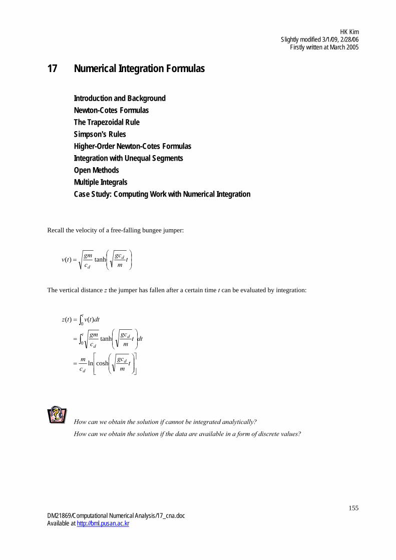
Recall the velocity of a free-falling bungee jumper:

t

m

gc

c

gmtv d

d

tanh)(

The vertical distance z the jumper has fallen after a certain time t can be evaluated by integration:

tm

gc

c

m

dttm

gc

c

gm

dttvtz

d

d

t d

d

t

coshln

tanh

)()(

0

0

How can we obtain the solution if cannot be integrated analytically?

How can we obtain the solution if the data are available in a form of discrete values?




156

Introduction and Background

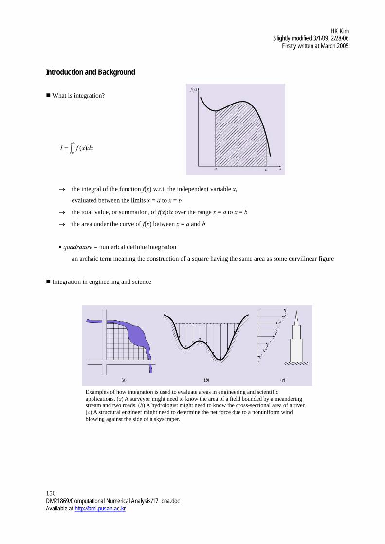
What is integration?

b

adxxfI )(

the integral of the function f(x) w.r.t. the independent variable x,

evaluated between the limits x = a to x = b

the total value, or summation, of f(x)dx over the range x = a to x = b

the area under the curve of f(x) between x = a and b

quadrature = numerical definite integration

an archaic term meaning the construction of a square having the same area as some curvilinear figure

Integration in engineering and science

Examples of how integration is used to evaluate areas in engineering and scientific applications. (a) A surveyor might need to know the area of a field bounded by a meandering stream and two roads. (b) A hydrologist might need to know the cross-sectional area of a river. (c) A structural engineer might need to determine the net force due to a nonuniform wind blowing against the side of a skyscraper.




157

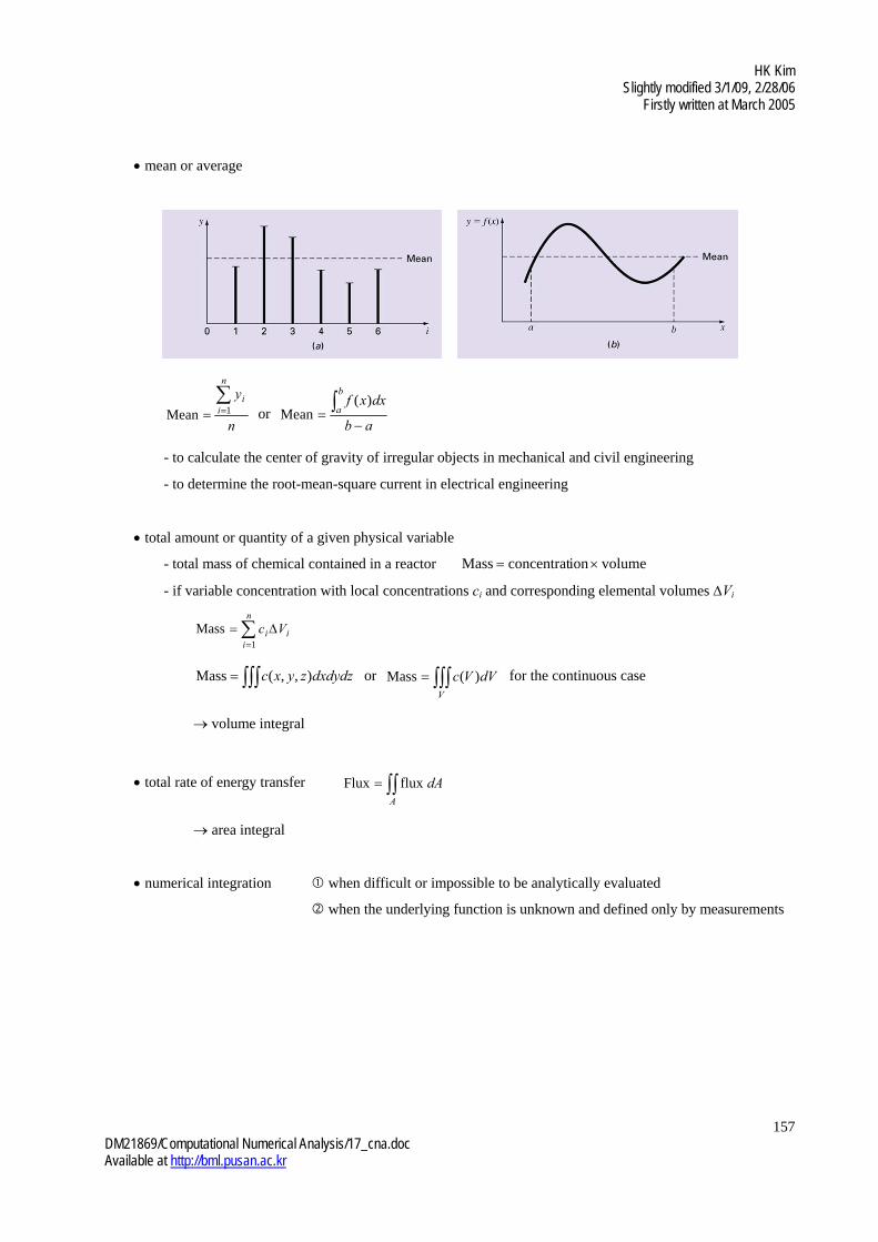
mean or average

n

yn

ii

1Mean or ab

dxxfb

a

)(

Mean

- to calculate the center of gravity of irregular objects in mechanical and civil engineering

- to determine the root-mean-square current in electrical engineering

total amount or quantity of a given physical variable

- total mass of chemical contained in a reactor volumeion concentratMass

- if variable concentration with local concentrations ci and corresponding elemental volumes Vi

n

iii Vc

1

Mass

dxdydzzyxc ),,(Mass or V

dVVc )(Mass for the continuous case

volume integral

total rate of energy transfer A

dAflux Flux

area integral

numerical integration when difficult or impossible to be analytically evaluated

when the underlying function is unknown and defined only by measurements




158

Newton-Cotes Formulas

the most common numerical integration schemes

based on the strategy of replacing a complicated function or tabulated data with a polynomial

b

a n

b

adxxfdxxfI )()(

where nn

nnn xaxaxaaxf

1110)(

also approximated using a series of polynomials (straight line or higher-order polynomial)

applied piecewise to the function or data over segments of constant length

closed vs. open forms of Newton-Cotes formulas

- closed forms: when knowing the data points at the beginning and end of the limits

- open forms: when integration limits extend beyond the range of the data

The approximation of an integral by the area under (a) a straight line and (b) a parabola.

The approximation of an integral by the area under three straight-line segments.

The difference between (a) closed and (b) open integration formulas.




159

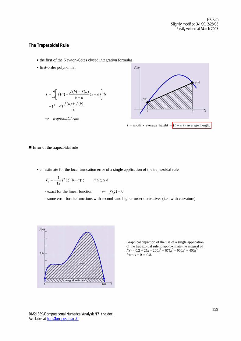
The Trapezoidal Rule

the first of the Newton-Cotes closed integration formulas

first-order polynomial

2

)()()(

)()()(

)(

bfafab

dxaxab

afbfafI

b

a

trapezoidal rule

height average )( height average width abI

Error of the trapezoidal rule

an estimate for the local truncation error of a single application of the trapezoidal rule

3))((12

1abξfEt ; a b

- exact for the linear function f''() = 0

- some error for the functions with second- and higher-order derivatives (i.e., with curvature)

Graphical depiction of the use of a single application of the trapezoidal rule to approximate the integral of f(x) = 0.2 + 25x – 200x2 + 675x3 – 900x4 + 400x5 from x = 0 to 0.8.




160

Example --------------------------------------------------------------------------------------------------------------------

Use the trapezoidal rule to numerically integrate 5432 400900675200252.0)( xxxxxxf from a = 0 to

b = 0.8. Note that the exact value is 1.640533.

Sol.)

1728.02

232.02.0)08.0(

I Et = 1.640533 – 0.1728 = 1.467733 t = 89.5%

An approximate error estimate 32 000,8800,10050,4400)( xxxxf

6008.0

)000,8800,10050,4400()(

8.0

0

32

dxxxx

xf

56.2)8.0)(60(12

1 3 aE

--------------------------------------------------------------------------------------------------------------------------------------------

How can we improve the accuracy of the trapezoidal rule?

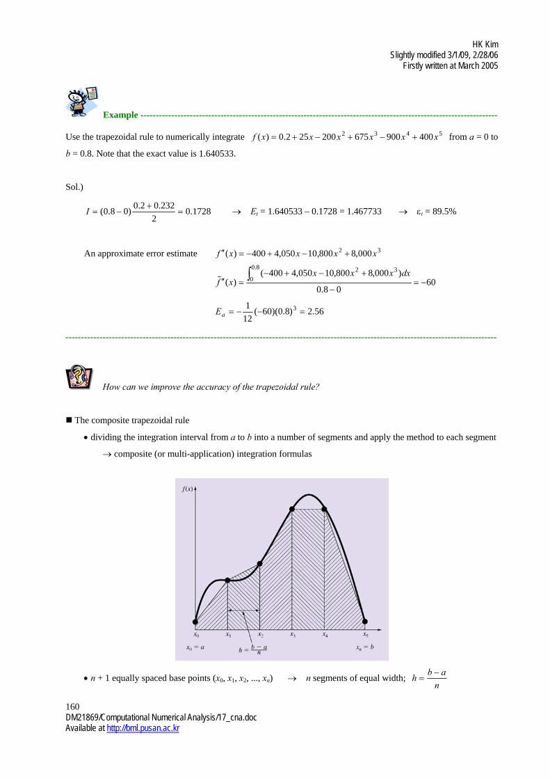
The composite trapezoidal rule

dividing the integration interval from a to b into a number of segments and apply the method to each segment

composite (or multi-application) integration formulas

n + 1 equally spaced base points (x0, x1, x2, ..., xn) n segments of equal width; n

abh




161

If a = x0 and b = xn;

n

n

x

x

x

x

x

xdxxfdxxfdxxfI

1

2

1

1

0

)()()(

Substituting the trapezoidal rule,

2

)()(

2

)()(

2

)()( 12110 nn xfxfh

xfxfh

xfxfhI

or

)()(2)(

2

1

10 n

n

ii xfxfxf

hI

or

height Average

1

10

Width2

)()(2)(

)(n

xfxfxf

abIn

n

ii

where the average height represents a weighted average of the function values.

an error for the composite trapezoidal rule (obtained by summing the individual errors for each segment)

n

iit ξf

n

abE

13

3

)(12

)(

or fn

abEa

2

3

12

)(

n

ξff

n

ii

1

)( and fnξf

n

ii

1

)(

if the number of segments is doubled, the truncation error will be quartered! (Ea ~ 1/n2)

Example --------------------------------------------------------------------------------------------------------------------

Use the two-segment trapezoidal rule to estimate the integral of

5432 400900675200252.0)( xxxxxxf

from a = 0 to b = 0.8. Recall that the exact value is 1.640533.

Sol.)

For n = 2 (h = 0.4):

232.0)8.0( 456.2)4.0( 2.0)0( fff

0688.14

232.0)456.2(22.08.0

I

%9.34 57173.00688.1640533.1 tt εE

64.0)60()2(12

8.02

2

aE

--------------------------------------------------------------------------------------------------------------------------------------------




162

<Results for the composite trapezoidal rule to estimate the integral of

f(x) = 0.2 + 25x – 200x2 + 675x3 – 900x4 from x = 0 to 8. The exact value is 1.640533.>

n h I t (%)

2 3 4 5 6 7 8 9

10

0.4 0.2667

0.2 0.16

0.1333 0.1143

0.1 0.0889 0.08

1.0688 1.3695 1.4848 1.5399 1.5703 1.5887 1.6008 1.6091 1.6150

34.9 16.5 9.5 6.1 4.3 3.2 2.4 1.9 1.6

notice how the error decreases as the number of segments increases

notice that the rate of decrease is gradual

MATLAB M-file: trap

<An M-file to implement the composite trapezoidal rule>




163

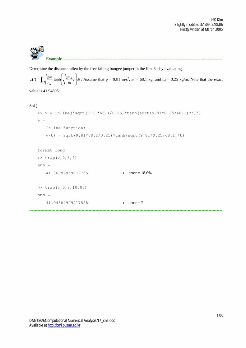
Example --------------------------------------------------------------------------------------------------------------------

Determine the distance fallen by the free-falling bungee jumper in the first 3 s by evaluating

t d

d

dttm

gc

c

gmtz

0tanh)( . Assume that g = 9.81 m/s2, m = 68.1 kg, and cd = 0.25 kg/m. Note that the exact

value is 41.94805.

Sol.)

>> v = inline('sqrt(9.81*68.1/0.25)*tanh(sqrt(9.81*0.25/68.1)*t)')

v =

Inline function:

v(t) = sqrt(9.81*68.1/0.25)*tanh(sqrt(9.81*0.25/68.1)*t)

format long

>> trap(v,0,3,5)

ans =

41.86992959072735 error = 18.6%

>> trap(v,0,3,10000)

ans =

41.94804999917528 error = ?

--------------------------------------------------------------------------------------------------------------------------------------------




164

Simpson's Rules

another way to obtain a more accurate estimate aside from the trapezoidal rule with finer segmentation

the formulas that result from taking the integrals under higher-order polynomials

Simpson's 1/3 rule

using a second-order polynomial

dxxfxxxx

xxxxxf

xxxx

xxxxxf

xxxx

xxxxI

x

x

)())((

))(()(

))((

))(()(

))((

))((2

1202

101

2101

200

2010

212

0

or )]()(4)([3 210 xfxfxfh

I or 6

)()(4)()( 210 xfxfxf

abI

where h = (b – a)/2

a = x0, b = x2, and x1 = (a + b)/2

- notice that the middle point is weighted by two-thirds and the two end points by one-sixth

a truncation error

)(90

1 )4(5 ξfhEt or )(2880

)( )4(5

ξfab

Et

h = (b – a)/2

- proportional to the "forth" derivative rather than the "third" one expected

third-order accurate or yielding exact results for cubic polynomials

even though derived from a parabola

(a) Graphical depiction of Simpson’s 1/3 rule: It consists of taking the area under a parabola connecting three points. (b) Graphical depiction of Simpson’s 3/8 rule: It consists of taking the area under a cubic equation connecting four points.




165

Example --------------------------------------------------------------------------------------------------------------------

Use the Simpson's 1/3 rule to integrate

5432 400900675200252.0)( xxxxxxf


Sol.)

For n = 2 (h = 0.4):

232.0)8.0( 456.2)4.0( 2.0)0( fff

367467.16

232.0)456.2(42.08.0

I

%6.16 2730667.0367467.1640533.1 tt εE

~ 5 times more accurate than for a single application of the trapezoidal rule

2730667.0)2400(2880

8.0 5

aE

--------------------------------------------------------------------------------------------------------------------------------------------

The composite Simpson's 1/3 rule

to improve by dividing the integration interval into a number of segments of equal width

n

n

x

x

x

x

x

xdxxfdxxfdxxfI

2

4

2

2

0

)()()(

Substituting Simpson's 1/3 rule,

6

)()(4)(2

6

)()(4)(2

6

)()(4)(2 12432210 nnn xfxfxf

hxfxfxf

hxfxfxf

hI

or

n

xfxfxfxf

abI

n

n

jj

n

ii

3

)()(2)(4)(

)(

2

6,4,2

1

5,3,10

note that an "even" number of segments must be utilized

an error estimate: )4(4

5

180

)(f

n

abEa




166

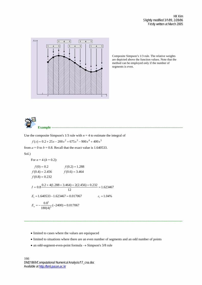
Example --------------------------------------------------------------------------------------------------------------------

Use the composite Simpson's 1/3 rule with n = 4 to estimate the integral of

5432 400900675200252.0)( xxxxxxf


Sol.)

For n = 4 (h = 0.2):

232.0)8.0(

464.3)6.0( 456.2)4.0(

288.1)2.0( 2.0)0(

f

ff

ff

623467.112

232.0)456.2(2)464.3288.1(42.08.0

I

%04.1 017067.0623467.1640533.1 tt εE

017067.0)2400()4(180

8.04

5

aE

--------------------------------------------------------------------------------------------------------------------------------------------

limited to cases where the values are equispaced

limited to situations where there are an even number of segments and an odd number of points

an odd-segment-even-point formula Simpson's 3/8 rule

Composite Simpson’s 1/3 rule. The relative weights are depicted above the function values. Note that the method can be employed only if the number of segments is even.




167

Simpson's 3/8 rule

the third Newton-Cotes closed integration formula

using a third-order Lagrange polynomial

)]()(3)(3)([8

33210 xfxfxfxf

hI

or 8

)()(3)(3)()( 3210 xfxfxfxf

abI

where h = (b – a)/3

an error: )(80

3 )4(5 ξfhEt or )(6480

)( )4(5

ξfab

Et

- the "third"-order accuracy with "four" points

- preferred Simpson's 1/3 rule because of the "third"-order accuracy with "three" points

utilizable when the number of segments is odd

Example --------------------------------------------------------------------------------------------------------------------

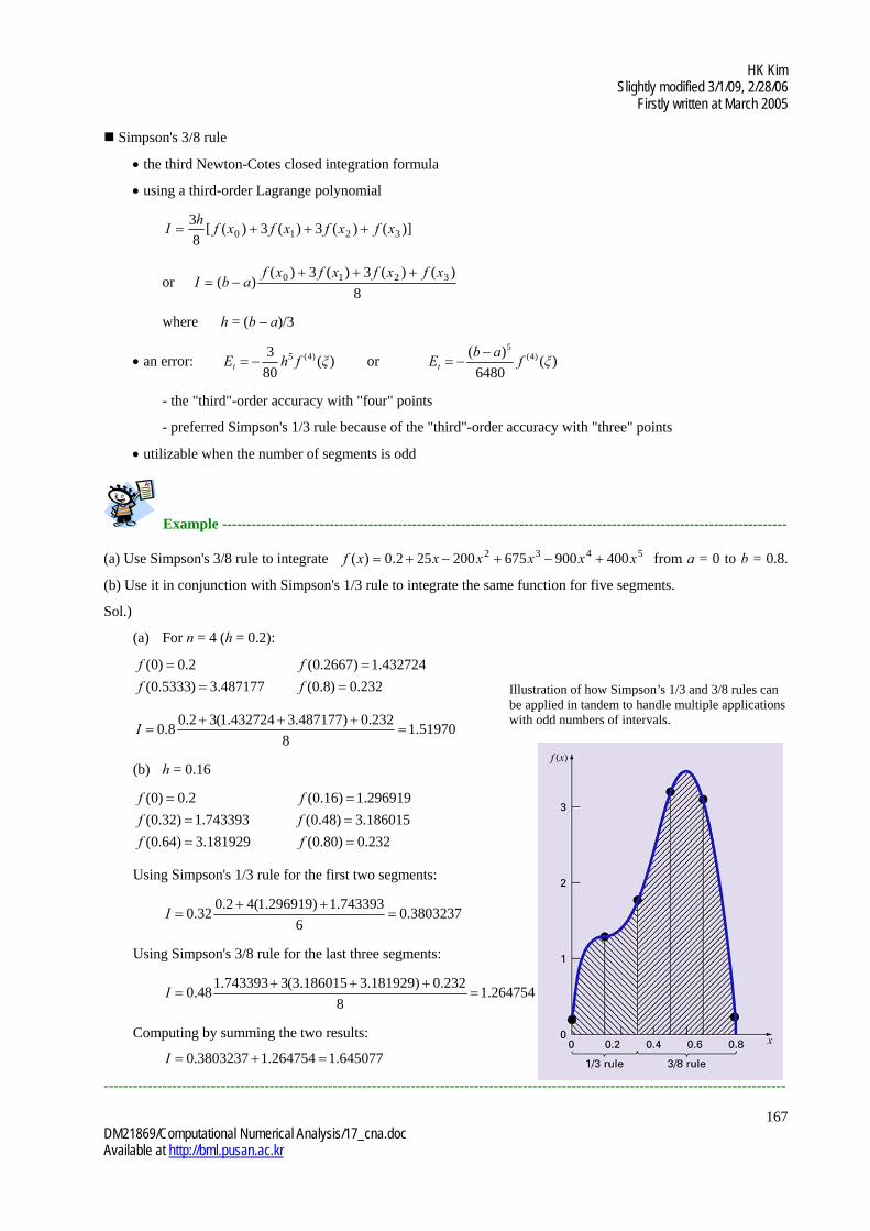
(a) Use Simpson's 3/8 rule to integrate 5432 400900675200252.0)( xxxxxxf from a = 0 to b = 0.8.

(b) Use it in conjunction with Simpson's 1/3 rule to integrate the same function for five segments.

Sol.)

(a) For n = 4 (h = 0.2):

232.0)8.0( 487177.3)5333.0(

432724.1)2667.0( 2.0)0(

ff

ff

51970.18

232.0)487177.3432724.1(32.08.0

I

(b) h = 0.16

232.0)80.0( 181929.3)64.0(

186015.3)48.0( 743393.1)32.0(

296919.1)16.0( 2.0)0(

ff

ff

ff

Using Simpson's 1/3 rule for the first two segments:

3803237.06

743393.1)296919.1(42.032.0

I

Using Simpson's 3/8 rule for the last three segments:

264754.18

232.0)181929.3186015.3(3743393.148.0

I

Computing by summing the two results:

645077.1264754.13803237.0 I

--------------------------------------------------------------------------------------------------------------------------------------------

Illustration of how Simpson’s 1/3 and 3/8 rules can be applied in tandem to handle multiple applications with odd numbers of intervals.




168

Higher-Order Newton-Cotes Formulas

<Newton-Cotes closed integration formulas. The step size is given by h = (b – a)/n>

Segments (n)

Points Name Formula Truncation

Error

1 2 Trapezoidal

rule 2

)()()( 10 xfxf

ab

)(12/1 3 fh

2 3 Simpson's 1/3 rule 6

)()(4)()( 210 xfxfxf

ab

)(90/1 )4(5 fh

3 4 Simpson's 3/8 rule 8

)()(3)(3)()( 3210 xfxfxfxf

ab

)(80/3 )4(5 fh

4 5 Boole's

rule 90

)(7)(32)(12)(32)(7)( 43210 xfxfxfxfxf

ab

)(945/8 )6(7 fh

5 6 288

)(19)(75)(50)(50)(75)(19)( 543210 xfxfxfxfxfxf

ab

)(096,12/275 )6(7 fh

the even-segment-odd-point formulas are usually the methods of preference

the higher-order (> four-point) formulas are not commonly used in engineering and science practice

Simpson's rules are sufficient for most applications (with an improved accuracy using the composite version)

How can we apply the numerical integration to the unequispaced data (e.g., experimentally derived data)?

Integration with Unequal Segments

applying the trapezoidal rule to each segment and summing the results

2

)()(

2

)()(

2

)()( 1212

101

nnn

xfxfh

xfxfh

xfxfhI

where hi = the width of segment i

- similar to the composite trapezoidal rule in which the h's are constant

Example --------------------------------------------------------------------------------------------------------------------

Determine the integral for the following data. Note that the correct answer is 1.640533.

x f(x) x f(x) 0.00 0.12 0.22 0.32 0.36 0.40

0.200000 1.309729 1.305241 1.743393 2.074903 2.456000

0.44 0.54 0.64 0.70 0.80

2.842985 3.507297 3.181929 2.363000 2.32000

Sol.)

594801.12

232.0363.210.0

2

305241.1309729.110.0

2

309729.12.012.0

I t = 2.8%

--------------------------------------------------------------------------------------------------------------------------------------------




169

MATLAB M-file: trapuneq

<An M-file to implement the trapezoidal rule for unequally spaced data>

>> x = [0 .12 .22 .32 .36 .4 .44 .54 .64 .7 .8]

>> y = 0.2+25*x-200*x.^2+675.^3-900*x.^4+400*x.^5

>> trapuneq(x,y)

ans =

1.5948

MATLAB M-file: trapz

a built-in function

>> x = [0 .12 .22 .32 .36 .4 .44 .54 .64 .7 .8]

>> y = 0.2+25*x-200*x.^2+675.^3-900*x.^4+400*x.^5

>> trapz(x,y)

ans =

1.5948




170

Open Methods

<Newton-Cotes open integration formulas. The step size is given by h = (b – a)/n>

Segments (n)

Points Name Formula Truncation

Error

2 1 Midpoint method

)()( 1xfab )(3/1 3 fh

3 2 2

)()()( 21 xfxf

ab

)(4/3 3 fh

4 3 3

)(2)(1)(2)( 321 xfxfxf

ab

)(45/14 )4(5 fh

5 4 24

)(11)()()(11)( 4321 xfxfxfxf

ab

)(144/95 )4(5 fh

6 5 20

)(11)(14)(26)(14)(11)( 04321 xfxfxfxfxf

ab

)(140/41 )6(7 fh

the even-segment-odd-point formulas are usually the methods of preference

not often used for definite integration but utilizable for analyzing improper integrals

useful for analyzing improper integrals

relevant to methods for solving ordinary differential equations

Multiple Integrals

the average of a two-dimensional function

))((

),(

abcd

dydxyxff

d

c

b

a

double integral:

b

a

d

c

d

c

b

adxdyyxfdydxyxf ),(),(

- not importance in the order of integration

Double integral as the area under the function surface.




171

Example --------------------------------------------------------------------------------------------------------------------

Suppose that the temperature of a rectangular heated plate is described by the following function:

40222),( 22 yxxxyyxT

If the plate is 8 m long (x dimension) and 6 m wide (y dimension), compute the average temperature.

Sol.)

--------------------------------------------------------------------------------------------------------------------------------------------

MATLAB M-file: dblquad and triplequad

q = dblquad(fun, xmin, xmax, ymin, ymax, tol)

>> q = dblquad(@(x,y) 2*x*y+2*x-x.^2-2*y.^2+72,0,8,0,6)

q =

2816

Numerical evaluation of a double integral using the two-segment trapezoidal rule.




172

Documents

17 Numerical Integration Formulas - Welcome|Radiation …bml.pusan.ac.kr/resources/17_cna.pdf · · 2012-03-0817 Numerical Integration Formulas ... Examples of how integration is