Embed Size (px)
Citation preview

American Institute of Aeronautics and Astronautics
1
150 kW Class Solar Electric Propulsion Spacecraft
Power Architecture Model
Jeffrey T. Csank1, Michael V. Aulisio2
NASA Glenn Research Center, Cleveland, OH, 44135, USA
and
Benjamin Loop3
PC Krause and Associates, Inc., 3000 Kent Ave, Suite C1-100, West Lafayette, IN 47906, USA
The National Aeronautics and Space Administration (NASA) Solar Electric Propulsion
Technology Demonstration Mission (SEP TDM), in conjunction with PC Krause and
Associates, has created a Simulink-based power architecture model for a 50 kilo-Watt (kW)
solar electric propulsion system. NASA has extended this model to investigate 150 kW solar
electric propulsion systems. Increasing the power capability to 150 kW is an intermediate step
to the anticipated power requirements for Mars and other deep space applications. The high-
power solar electric propulsion capability has been identified as a critical part of NASA’s
future beyond-low-Earth-orbit for human-crewed exploration missions. This paper presents
four versions of a 150 kW architecture, simulation results, and a discussion of their merits.
Nomenclature
AEPS Advanced Electric Propulsion System
ARRM Asteroid Redirect Robotic Mission
DDCU DC-DC Converter Unit
DSG Deep Space Gateway
HET Hall Effect Thrusters
IPS Ion Propulsion System
ISS International Space Station
PDU Power Distribution Unit
PPB Power and Propulsion Bus
PPU Power Processor Unit
RBI Remote Bus Interrupter
SA Solar Array
SEP Solar Electric Propulsion
SEPM Solar Electric Propulsion Module
SSU Sequential Shunt Unit
I. Introduction
HE National Aeronautics and Space Administration (NASA), in conjunction with PC Krause and Associates, has
created a power architecture model for a 50 kW class Government reference design of the Solar Electric
Propulsion Module (SEPM) of the Asteroid Redirect Robotic Mission (ARRM).1 This vehicle and power system was
originally designed to power a high-power solar electric propulsion (SEP) system to return an asteroidal mass for
rendezvous and characterization in a companion human-crewed mission. NASA is also evaluating applicability of a
similar SEP system to that of the power and propulsion bus (PPB) of the Deep Space Gateway (DSG). The DSG will
1 Electrical Engineer, Power Management and Distribution Branch, [email protected], AIAA Sr. Member 2 Electrical Engineer, Power Management and Distribution Branch, [email protected] 3 Director of Engineering Services, PC Krause and Associates, [email protected]
T
https://ntrs.nasa.gov/search.jsp?R=20170007962 2018-07-17T05:55:43+00:00Z

American Institute of Aeronautics and Astronautics
2
be used to perform missions in cislunar space, and the PPB will be used for station keeping and the ability to transfer
among a family of orbits in the lunar vicinity to enable a variety of missions (surface of the moon, departure from high
lunar orbit to other destinations in the solar system).5 As an extension, NASA is investigating higher power
architectures for missions applicable to deep space transportation, such as to Mars. Higher-Power SEP is enabling for
these deep space missions as it is necessary to minimize the time spent in transportation from cislunar space to the
Mars surface.
The 150 kW power system uses an architecture similar to the 50 kW system as the foundation for the model.
Propulsion strings of 12.5 kW are implemented as basic building blocks. Flight versions of these electric propulsion
strings are being developed under the NASA SEP TDM-led Advanced Electric Propulsion System (AEPS) Project.
The power system architecture consists of twelve propulsion strings, providing roughly 150 kW of power for
propulsion, and two additional 2.5 kW branch switches for distributing power to avionics and other vehicle support
systems totaling 155 kW of power. Each propulsion string includes a power processor unit (PPU), which converts the
solar array generated power into the various regulated currents and voltages required to start and operate the Hall
Effect Thrusters (HET).
This paper compares four different architectures. The first architecture contains two solar arrays connected to a
single bus which distributes power to twelve propulsion strings and two avionics and support strings. The second
architecture is a segmented system in which a solar array powers a single bus which powers six power strings and a
single avionics and support system string. The remaining two architectures are regulated versions of the first two
architectures where a sequential shunt unit is added between the solar array and the bus to regulate the voltage to the
bus by adding a simulated load to the system. A simulation study illustrates the feasibility of each system operating
under multiple conditions. The simulations have been developed in the MATLAB® / Simulink ®, the MathWorks
Inc., environment using a custom Simulink International Space Station (ISS) model library developed by PC Krause
and Associates, Inc. The ISS model library contains MATLAB functions and Simulink blocks to represent the salient
performance characteristics of the ISS electrical power system to support the development of intelligent energy
management controls.2 In particular, the model library is capable of facilitating stability analysis through its prediction
of transient effects. Both large signal and small signal stability effects can be evaluated (see, for example, Section II-
C below). The basic structure of the SEP spacecraft power architecture Simulink model consists of solar array blocks,
from the ISS library, connected to one or more loads, including both the propulsion strings and support power. Each
propulsion power string is designated to draw 12.5 kW at 100 Vdc. For this study, it is assumed that there will be two
solar arrays each capable of providing approximately 75-80 kW of power and has an irradiance of 1.380 kW/m2 at
any moment in time. The solar array is configured with 210 cells in each string, 310 parallel strings to deliver the
required power at the appropriate voltage level. In steady-state and full load, each solar array provides 79.4 kW of
power at 117.8 V and 673.95 amperes.
For electric propulsion vehicles, electric power is required for both driving the vehicle and powering all the
avionics and vehicle support systems. Therefore the vehicle requires high availability of electrical power. When
considering some of the possible support systems, such as life support for manned space vehicles, continuous operation
of these systems is critical. The unanticipated interruption of electric power availability is often the result of some
component failure, or fault, in the system. The goal is to design the system to be fault tolerant, or be able to withstand
a single failure without major consequence. Increasing the fault tolerance, or availability, usually requires increasing
the cost and complexity of the system. Taking advantage of partitioning and redundancy can help achieve fault
tolerance. Redundancy is adding additional components to the system to replace the failed components, whereas
partitioning ensures that a failure in one subsystem will not impact the other subsystems.3
II. 150kW Non-Segmented Power System
The 150 kW class non-segmented power system consists of twelve electric propulsion strings consuming 12.5 kW
of power with two additional branches dedicated for 2.5 kW of power each for avionics and other support systems.
This architecture features a common-bus which is supplied power from two solar arrays (SA-1, SA-2) and distributes
the 155 kW of power to the fourteen branches, reference Figure 1. Each propulsion string is connected to the solar
array (or bus) through a Remote Bus Interrupter (RBI) block, which acts as a switch and is either open or closed. In
Simulink, each propulsion string is represented by a constant power DC-DC Converter Unit (DDCU), which converts
power from the source to the load at the desired voltages, connected to a constant power load. The DDCU and constant
power load for each propulsion string is configured to represent the Ion Propulsion System (IPS) Power Processing
Unit (PPU) function and power demand. The avionics and support power loads consist of a DDCU connected to a
constant power load at 100 V and another DDCU which is connected to a constant power load at 30 V, which models
the loads attached to a 100 V Power Distribution Unit (PDU) and 30 V PDU. At full power the solar arrays provide

American Institute of Aeronautics and Astronautics
3
the bus with 158.83 kW of total power including losses. This likely represents the simplest architecture of one such
class system and is presented as a starting point in this feasibility study.
A. Transient Response
Consider turning all twelve propulsion power strings on at exactly the same time. Before the power is turned on,
the solar arrays should be at or near the solar array open circuit voltage, which is approximately 136 volts, and only
providing power to the two 2.5 kW avionics and support system strings. At a simulation time of 4 seconds, a single
step command is given to command all the propulsion string loads to turn on at the same time. When this occurs, the
current out of and power to the bus from the solar arrays increases and the solar array voltages decrease. The solar
array voltage for SA-1 (top plot) and total power supplied by the array and total power consumed by the loads (bottom
plot) is shown in Figure 2. Figure 2 shows that when the loads are powered on the power system goes through a short
transient, approximately 3 milliseconds, and the solar array settles to a lower voltage at 46 volts and produces
approximately 80 kW of power, which is less than the designed 155 kW of power. The existence and stability issues
regarding this low-voltage/low-power state is discussed in more detail in Section C below.
To decrease the instantaneous demand on the
generation and distribution systems, a 1
millisecond delay is inserted between the
commands to each RBI and provide power to each
propulsion string incrementally. The solar array
voltage and total power both generated and
consumed, is shown in the left plot of Figure 3. In
this scenario, it takes approximately 12
milliseconds to deliver power to all the loads and
allows for the solar arrays to operate at the full
load voltage, 117.8 volts, and delivers the
requested 155 kW of power. This scheme allows
for the power system to deliver the required power
and voltage but does also allow high power and
voltage swings during the 12 milliseconds power
up phase.
An alternative solution is to increase the
transition time from 1 millisecond to 20
Figure 1. The 150kW non-segmented architecture.
RBI1
RBI2
RBI3
RBI12
IPS PPU 1
IPS PPU 2
IPS PPU 3
IPS PPU 12
100V PDU
12.5 kW
12.5 kW
12.5 kW
12.5 kW
2.5 kW
2.5 kW100V PDU
28V PDU
28V PDU
Thruster
Avionics and support system power
SA-1
SA-2
… …
Figure 2. Solar array voltage response (top plot) and total
array and load power (bottom) when turning all
propulsion power strings on.
3.995 4 4.005 4.01 4.0150
50
100
150
SA
-1, V
Time, s
3.995 4 4.005 4.01 4.0150
100
200
Tota
l Po
we
r, k
W
Time, s
Load
Array
American Institute of Aeronautics and Astronautics
4
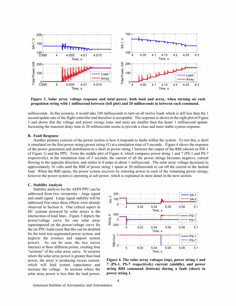
milliseconds. In this scenario, it would take 240 milliseconds to turn on all twelve loads which is still less than the 1
second update rate of the flight controller and therefore is acceptable. The response is shown in the right plot of Figure
3 and shows that the voltage and power swings (max and min) are smaller than the faster 1 millisecond update.
Increasing the transient delay time to 20 milliseconds seems to provide a clear and more stable system response.
B. Fault Response
Another primary concern of the power system is how it responds to faults within the system. To test this, a short
is simulated on the first power string (power string #1) at a simulation time of 5 seconds. Figure 4 shows the response
of the power generation and distribution to a short in power string 1 between the output of the RBI (shown as SW-1
of Figure 1) and the PPU. From the middle plot of Figure 4, which compares power string 1 and 7 (PS-1 and PS-7
respectively), at the simulation time of 5 seconds, the current of all the power strings becomes negative, current
flowing in the opposite direction, and settles to 0 amps in about 1 millisecond. The solar array voltage decreases to
approximately 16 volts until the RBI of power string 1 opens at 50 milliseconds to cut off the current to the faulted
load. When the RBI opens, the power system recovers by restoring power to each of the remaining power strings,
however the power system is operating at sub power, which is explained in more detail in the next section.
C. Stability Analysis
Stability analysis for the AEPS PPU can be
addressed from two viewpoints – large signal
and small signal. Large signal stability will be
addressed first since these effects were already
observed in Section A. One critical aspect in
DC systems powered by solar arrays is the
intersection of load lines. Figure 5 depicts the
power/voltage curve for one solar array
superimposed on the power/voltage curve for
the six PPU loads (note that this can be doubled
for the total non-segmented power system, and
neglects the avionics and support system
power). As can be seen, the two curves
intersect at three different points, creating four
“sections” of the solar array curve. In sections
where the solar array power is greater than load
power, the array is producing excess current,
which will feed system capacitance and
increase the voltage. In sections where the
solar array power is less than the load power,
Figure 3. Solar array voltage response and total power, both load and array, when turning on each
propulsion string with 1 millisecond between (left plot) and 20 milliseconds in between each command.
3.995 4 4.005 4.01 4.015100
150
200S
A-1
, V
Time, s
3.995 4 4.005 4.01 4.0150
100
200
Tota
l Po
we
r, k
W
Time, s
Load
Array
4 4.05 4.1 4.15 4.2 4.25 4.3100
150
SA
-1, V
Time, s
4 4.05 4.1 4.15 4.2 4.25 4.30
100
200
Tota
l Po
we
r, k
W
Time, s
Load
Array
Figure 4. The solar array voltages (top), power string 1 and
7 (PS-1, PS-7 respectively) current (middle), and power
string RBI command (bottom) during a fault (short) in
power string 1.
5 5.02 5.04 5.06 5.08 5.10
100
200
SA
, V
Time, s
5 5.02 5.04 5.06 5.08 5.1-200
0
200
Str
ing, A
Time, s
5 5.02 5.04 5.06 5.08 5.10
1
RB
I C
md
Time, s
SA-1
SA-2
PS-1
PS-7
PS-1
PS-7

American Institute of Aeronautics and Astronautics
5
current will be drawn from the system capacitance
and decrease the voltage. Following this idea, arrows
can be drawn in the diagram to indicate the direction
of voltage change in each section. The intersection
points of the array and load curves indicate
equilibrium points, where the source and load powers
are balanced. The equilibrium points with arrows
pointing towards each other are stable, whereas
intersection points with arrows pointing away from
each other are unstable (since a small perturbation
will move it further from the equilibrium point).
The simulation results in Figure 2 depict a
scenario in which the transient (turning all strings at
full load simultaneously) is large enough to push the
bus voltage below the unstable equilibrium point, and
it settles at the low-voltage/low-power stable
equilibrium point. Note that the fault scenario in
Section B depicts a similar situation where the short
pushes the bus voltage below the unstable equilibrium point and it settles to another low power voltage that is slightly
higher. The diagram in Figure 6 depicts the bus voltage transient from Figure 2 (black line) superimposed on the solar
array’s power/voltage curve (extended into a third dimension with time). The gray line is the approximate location of
the unstable equilibrium. As can be seen this point is exceeded during the transient, and the array voltage cannot
recover to the high-voltage equilibrium. The bus voltage transient associated with the 20 ms load steps (seen in
Figure 3) has been superimposed on the array power/voltage curve in Figure 7. As can be seen, for this case, the more
gradual transient does not reach the critical voltage. Consequently, the bus voltage stabilizes to the desired equilibrium
point. Adjusting the foldback points for the DDCU/load combination could eliminate the undesirable equilibrium
points, and then the dynamic (small signal) stability of the desirable equilibrium point would be the only remaining
concern.
PCKA’s ISS model library also includes a tool to facilitate the calculation of eigenvalues for the linearized small
signal system dynamics. This was applied to the non-segmented power system to evaluate dynamic stability of the
system. The full system Jacobian matrix was calculated at 10 load levels in equal steps from 10% up to 100% for all
12 PPUs. Then, the eigenvalues of the system were calculated from the Jacobian matrices. Most eigenvalues do not
change appreciably as a result of changing the load; however, the eigenvalues associated with the input filter capacitors
on the DDCUs were found to change significantly (associating states with particular eigenvalues was done by
calculating participation factors). The change in this particular eigenvalue due to the load level is depicted in Figure
8. Therein, it can be seen that the eigenvalues change from oscillatory (with non-zero imaginary parts) to purely real
Figure 5. Power/voltage curves for solar array and
PPU loads.
Figure 6. Step load transient of array power/voltage relationship.

American Institute of Aeronautics and Astronautics
6
and it moves toward the origin. This trajectory of eigenvalues is moving toward instability (positive real part);
however, instability is not reached at full load. This indicates that dynamic stability is not a concern for the system as
designed. The issues with large-signal stability observed with the unregulated systems can be largely avoided in the
regulated case. The SSU can maintain the array at a high-current voltage level and quickly route the shunted current
to loads during a load step-on transient. As long as the total load does not exceed the peak power of the arrays, the
voltage can be maintained above the critical point corresponding to the unstable equilibrium point. The effects of
increasing load on the small signal stability were also examined. The black markers in Figure 8 show the equivalent
eigenvalues for C2 for the regulated case. With the bus voltage held nearly fixed by the regulators, these eigenvalues
do not move nearly as much as the unregulated case. It was found that eigenvalues involving the SSU controller and
the terminal capacitor (C1) do change significantly. They are depicted in Figure 9. These eigenvalues do move toward
the imaginary axis, but as above, do not cross, so the system remains stable.
Figure 7 Sequential load transient of array power/voltage relationship.
Figure 8 DDCU input filter eigenvalue sensitivity to load power.
Increasing load
Increasing load
American Institute of Aeronautics and Astronautics
7
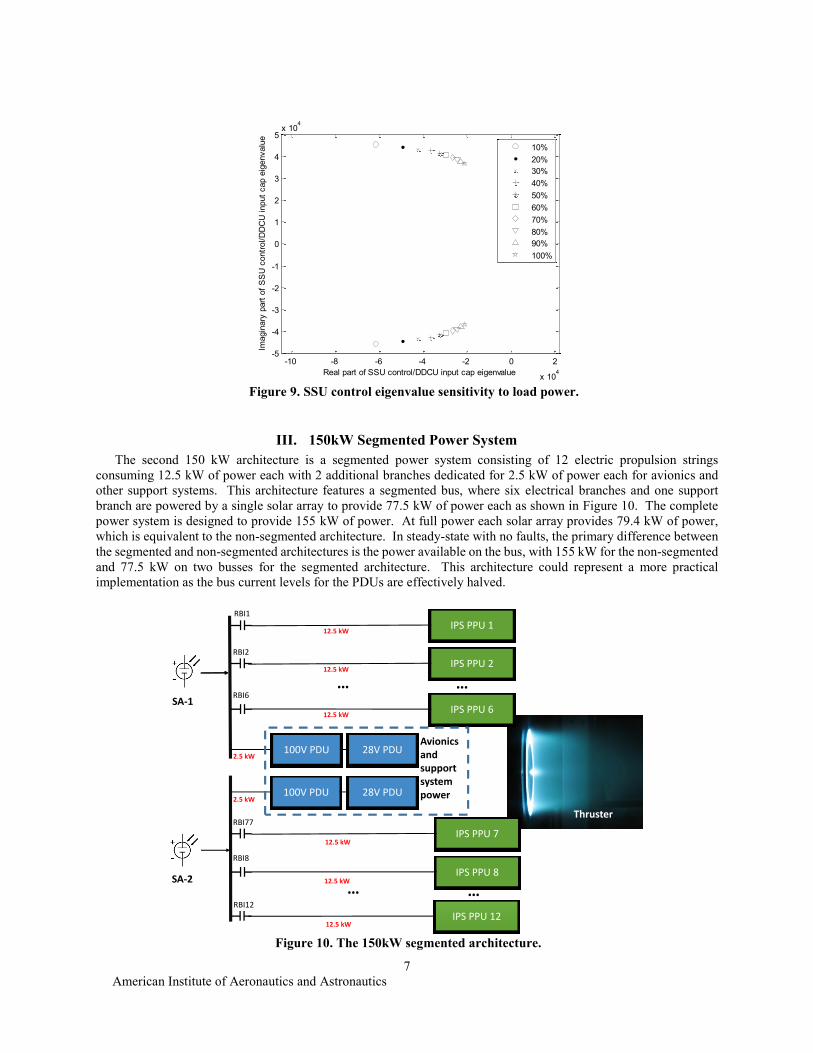
III. 150kW Segmented Power System
The second 150 kW architecture is a segmented power system consisting of 12 electric propulsion strings
consuming 12.5 kW of power each with 2 additional branches dedicated for 2.5 kW of power each for avionics and
other support systems. This architecture features a segmented bus, where six electrical branches and one support
branch are powered by a single solar array to provide 77.5 kW of power each as shown in Figure 10. The complete
power system is designed to provide 155 kW of power. At full power each solar array provides 79.4 kW of power,
which is equivalent to the non-segmented architecture. In steady-state with no faults, the primary difference between
the segmented and non-segmented architectures is the power available on the bus, with 155 kW for the non-segmented
and 77.5 kW on two busses for the segmented architecture. This architecture could represent a more practical
implementation as the bus current levels for the PDUs are effectively halved.
Figure 10. The 150kW segmented architecture.
RBI1
RBI2
RBI6
RBI12
IPS PPU 1
IPS PPU 2
IPS PPU 6
IPS PPU 12
100V PDU
12.5 kW
12.5 kW
12.5 kW
12.5 kW
2.5 kW
2.5 kW100V PDU
28V PDU
28V PDU
Avionics and support system power
SA-1
SA-2
RBI77
RBI8
IPS PPU 7
IPS PPU 8
12.5 kW
12.5 kW
… …
… …
Thruster
Figure 9. SSU control eigenvalue sensitivity to load power.
-10 -8 -6 -4 -2 0 2
x 104
-5
-4
-3
-2
-1
0
1
2
3
4
5x 10
4
Real part of SSU control/DDCU input cap eigenvalue
Imagin
ary
part
of
SS
U c
ontr
ol/D
DC
U input
cap e
igenvalu
e
10%
20%
30%
40%
50%
60%
70%
80%
90%
100%

American Institute of Aeronautics and Astronautics
8
A. Transient Response
The transient response of the segmented
power system when turning on all loads at one
time is shown in Figure 11 and is identical to the
non-segmented power system response shown in
Figure 2. In this instance, there is no difference in
the total power demand from the loads or total
power supplied from the source. Next, both a 1
millisecond and 20 millisecond delay are inserted
between turning on each power string. The
response with a 1 millisecond delay is shown in
the left plot of Figure 12 and the 20 millisecond
delay in the right plot of Figure 12. Figure 12
shows that adding the delay in the commands
cleans up the signal, which is the same trend as
shown with the non-segmented power
architecture and shown in Figure 4. However,
comparing the segmented (Figure 12) to the non-
segmented (Figure 4) architectures, the
segmented power architecture has smaller min
and max voltage and power values when turning
on each load. For the segmented case, turning on
load #7, which is the first load attached to the second solar array, does result in higher min and max values than turning
on the 7th power string of the non-segmented. This is because the 7th string of the segmented architecture is the first
load attached to the second solar array and will more closely resemble turning on load 1 of the segmented architecture.
The other option would have been to trade between the two solar arrays as the loads were turned on and in this case
the larger increase would not have been seen later in the sequence.
B. Fault Response
As with the non-segmented architecture, to test the fault response of the system a short is simulated on the first
power string (power string #1) at a simulation time of 5 seconds. For the segmented architecture, power strings 1
through 6 are attached to bus 1 and solar array 1, while power strings 7 through 12 are attached to bus 2 and solar
array 2. The voltages and currents associated with bus 1 decrease to zero when the short is inserted and remain at zero
Figure 11. Solar array voltage and total power for the
segmented power architecture when turning on all loads
at once.
3.995 4 4.005 4.01 4.0150
50
100
150
SA
-1, V
Time, s
3.995 4 4.005 4.01 4.0150
50
100
150
200
Tota
l Po
we
r, k
W
Time, s
Load
Array
a) b)
Figure 12. Solar array voltage and total power for the segmented power architecture with the loads turned
on in increments of a) 1 millisecond (left) and b) 20 milliseconds (right) between commands. All loads
connected to bus 1 are turned on before turning on the loads connected to bus 2.
3.995 4 4.005 4.01 4.01550
100
150
SA
-1, V
Time, s
3.995 4 4.005 4.01 4.0150
50
100
150
200
Tota
l Po
we
r, k
W
Time, s
Load
Array
4 4.05 4.1 4.15 4.2 4.25 4.3100
120
140
160
SA
-1, V
Time, s
4 4.05 4.1 4.15 4.2 4.25 4.30
50
100
150
200
Tota
l Po
we
r, k
W
Time, s
Load
Array

American Institute of Aeronautics and Astronautics
9
until RBI-1 opens and cuts off power,
allowing the voltage to increase. The
voltages and currents associated with
bus 2 remain untouched and still provide
power to the propulsion system and
support systems. With this architecture,
the system is able to restore the voltage
on the remaining operational loads
connected to bus 1 (loads 2 through 6) to
the same voltage as before the fault. In
this architecture, the fault does not cause
the bus voltage to drop below the critical
voltage. After the fault, there is less
total current draw from the solar array,
therefore solar array 1 will operate with
a slightly higher voltage than solar array
2.
C. Stability Analysis
From a mathematical perspective,
the stability analysis for the segmented
and non-segmented systems is identical;
therefore, the results in Section II-C apply to the segmented system as well.
IV. Regulated Architectures
A sequential shunt unit (SSU) can be added at the output of each solar array to provide a more stabilized output
voltage and power output. The SSU block is part of the ISS Simulink library toolbox and represents the behavior of
a sequential shut unit. The SSU regulates the bus voltage by supplying a resistive load which increases as the load
decreases to provide a constant voltage and load as done on the ISS.4 Figure 14 shows the solar array voltage and total
power of the a) non-segmented and b) segmented power architectures. With the SSU included in the power system,
the total power and solar array voltage is more consistent and has much smaller swings as the loads are turned on, as
shown in Figure 14.
Figure 13. Solar array voltages (top), power string current
(middle), and RBI commands (bottom) for the segmented power
architecture.
5 5.02 5.04 5.06 5.08 5.1-200
0
200
SA
, V
Time, s
5 5.02 5.04 5.06 5.08 5.1-200
0
200
Str
ing, A
Time, s
5 5.02 5.04 5.06 5.08 5.10
1
RB
I C
md
Time, s
SA-1
SA-2
PS-1
PS-7
PS-1
PS-7
a) b)
Figure 14. The solar array voltage and total power for the a) regulated non-segmented power architecture
(left) and b) the regulated segmented power architecture (right) to turning on all loads in 20 millisecond
increments.
4 4.05 4.1 4.15 4.2 4.25 4.398
100
102
104
SA
-1, V
Time, s
4 4.05 4.1 4.15 4.2 4.25 4.30
100
200
Tota
l Po
we
r, k
W
Time, s
Load
Array
4 4.05 4.1 4.15 4.2 4.25 4.395
100
105
SA
-1, V
Time, s
4 4.05 4.1 4.15 4.2 4.25 4.30
100
200
Tota
l Po
we
r, k
W
Time, s
Load
Array

American Institute of Aeronautics and Astronautics
10
Figure 15 compares the minimum and maximum voltages obtained when turning on an additional load and the
steady-state value obtained when the voltage settles. The top plots show the non-segmented power architecture while
the bottom plots show the segmented. The left plot (a) shows the systems without the SSU while the right plots (b)
show the results with the SSU at the output of each solar array. In the segmented case with no SSU, all the loads
connected to string 1 (solar array 1) are turned on before powering any loads attached to string 2, which is the reason
why the lowest minimum voltages are obtained when turning on loads 6 and 12 (last loads of each string) and why
turning on loads 1 and 7 results in the largest maximum voltage (first of each string).
The issues with large-signal stability observed with the unregulated systems can be largely avoided in the regulated
case. The SSU can maintain the array at a high-current voltage level and quickly route the shunted current to loads
during a load step-on transient. As long as the total load does not exceed the peak power of the arrays, the voltage
can be maintained above the critical point corresponding to the unstable equilibrium point. A fast-switching regulator
can also be an effective tool in stabilizing the small signal behavior of the system.
V. Discussion/Comparison
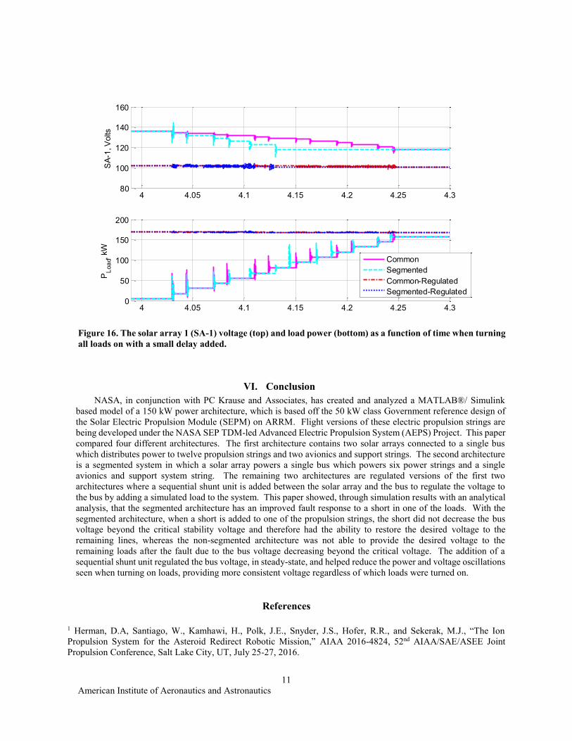
This paper looked at four different 150kW power systems, non-segmented, segmented, non-segmented regulated,
and segmented regulated. In each case, the numerical stability analysis provided the same results and will not be
discussed further in this section. The solar array voltage and power supplied to the loads as a function of time when
turning all loads on is shown in Figure 16. As shown in Figure 16 and in the prior sections, the regulated architecture
with the SSU unit provides a more constant power and voltage on the bus and removes the large power swings seen
when additional loads are added to the bus. This includes transient changes in the power demand from the loads. As
for the common versus segmented bus architecture with the power being regulated, there is not much difference in the
performance. The one advantage that the segmented architecture does provide is in a fault scenario on the power
generation side, such as a solar array failure, where all strings would not draw power from the remaining solar array.
In a segmented case, half the power strings would lose power and the other half would provide nominal power. This
is important when considering that avionics and life support systems need continuous power.
a) b)
Figure 15. The minimum, maximum, and steady-state voltages when turning on each load. The left plots a) show
the non-segmented (top) and segmented (bottom) with no SSU, while the right plots, b) shows the voltages with
the SSU included.
0 2 4 6 8 10 12100
120
140
160Non-segmented
Load turned on
Volta
ge
, V
Min
Max
SS
0 2 4 6 8 10 12100
120
140
160Segmented
Volta
ge
, V
Load turned on
0 2 4 6 8 10 12100
102
104Non-segmented
Load turned on
Volta
ge
, V
Min
Max
SS
0 2 4 6 8 10 1295
100
105Segmented
Volta
ge
, V
Load turned on
American Institute of Aeronautics and Astronautics
11
VI. Conclusion
NASA, in conjunction with PC Krause and Associates, has created and analyzed a MATLAB®/ Simulink
based model of a 150 kW power architecture, which is based off the 50 kW class Government reference design of
the Solar Electric Propulsion Module (SEPM) on ARRM. Flight versions of these electric propulsion strings are
being developed under the NASA SEP TDM-led Advanced Electric Propulsion System (AEPS) Project. This paper
compared four different architectures. The first architecture contains two solar arrays connected to a single bus
which distributes power to twelve propulsion strings and two avionics and support strings. The second architecture
is a segmented system in which a solar array powers a single bus which powers six power strings and a single
avionics and support system string. The remaining two architectures are regulated versions of the first two
architectures where a sequential shunt unit is added between the solar array and the bus to regulate the voltage to
the bus by adding a simulated load to the system. This paper showed, through simulation results with an analytical
analysis, that the segmented architecture has an improved fault response to a short in one of the loads. With the
segmented architecture, when a short is added to one of the propulsion strings, the short did not decrease the bus
voltage beyond the critical stability voltage and therefore had the ability to restore the desired voltage to the
remaining lines, whereas the non-segmented architecture was not able to provide the desired voltage to the
remaining loads after the fault due to the bus voltage decreasing beyond the critical voltage. The addition of a
sequential shunt unit regulated the bus voltage, in steady-state, and helped reduce the power and voltage oscillations
seen when turning on loads, providing more consistent voltage regardless of which loads were turned on.
References
1 Herman, D.A, Santiago, W., Kamhawi, H., Polk, J.E., Snyder, J.S., Hofer, R.R., and Sekerak, M.J., “The Ion
Propulsion System for the Asteroid Redirect Robotic Mission,” AIAA 2016-4824, 52nd AIAA/SAE/ASEE Joint
Propulsion Conference, Salt Lake City, UT, July 25-27, 2016.
Figure 16. The solar array 1 (SA-1) voltage (top) and load power (bottom) as a function of time when turning
all loads on with a small delay added.
4 4.05 4.1 4.15 4.2 4.25 4.380
100
120
140
160S
A-1
, V
olts
4 4.05 4.1 4.15 4.2 4.25 4.30
50
100
150
200
PL
oa
d, kW
Common
Segmented
Common-Regulated
Segmented-Regulated

American Institute of Aeronautics and Astronautics
12
2 Loop, B., “Simulation Environment for Power Management and Distribution Development,” SBIR Technologies
Workshop, Denver, CO, June 28, 2012. 3 White, R.V., “Fault Tolerance in Distributed Power Systems,” IEEE, International Conference on Power Electronics
(CIEP), MEXICO, San Luis, Potosi, October 16-19, 1995. 4 Wikipedia Contributors, “Electrical system of the International Space Station,” Wikipedia, The Free Encyclopedia,
https://en.wikipedia.org/wiki/Electrical_system_of_the_International_Space_Station#SSU, assessed March 30, 2017. 5 Gerstenmaier, W.H., “Progress in Defining the Deep Space Gateway and Transportation Plan,” Presentation to the
NASA Advisory Council, March 28, 2017.