January 28, 2002

15. The Simplest Integrals

15.1 INTRODUCTION

In Chapters 5 – 11 we constructed a Table of Derivatives, which is reproduced

in Appendix E. Each entry in the left column is a specific function f(x). The

corresponding entry in the right column is df/dx, or f ′(x).

We can immediately write the indefinite integral for any function in the

right column of the Table of Derivatives. If we call the function in the right

column g(x) [= f ′(x)] then the indefinite integral, or antiderivative, of g(x)

is f(x) + C by the fundamental theorem of calculus:∫

g(x)dx = f(x) + C, (15-1)

because df/dx = g(x). Here C is an unspecified constant, called the “constant

of integration.”

These are the simplest integrals—integrals of functions [ g(x) ] that are

easily recognized as derivatives [ f ′(x) ].

Example 1. What is the integral of 3x2?

Solution. Look for 3x2 in the right-hand column of the Table of Derivatives

in Appendix E. We find 3x2 as the derivative of x3. Thus the antiderivative

of 3x2 is x3 + C:∫

3x2dx = x3 + C, (15-2)

because the derivative of the function on the right-hand side of the equation

equals the integrand on the left-hand side. The constant C is arbitrary here,

because the derivative of any constant is 0.

Example 2. What is the integral of cosx?

Solution. Look for cosx in the right-hand column of the Table of Deriva-

tives in Appendix E. We find cosx as the derivative of sin x; so the antideriva-

tive, or indefinite integral, of cosx is sin x + C,∫

cosx dx = sin x + C. (15-3)

1

2 Chapter 15

Examples 1 and 2 are indefinite integrals. But what if we wanted a definite

integral? Recall from Sec. 14.5 that we can immediately evaluate a definite

integral if we know the indefinite integral. Suppose again that g(x) = df/dx,

so that the indefinite integral of g(x) is (15-1). Then the definite integral of

g(x) (with arbitrary endpoints a and b) is

∫ b

a

g(x)dx = f(x)|ba = f(b)− f(a) (15-4)

by Eq. (14-2). Equation (15-4) introduces a handy notation; for any function

f(x) and domain [a, b] of x,

f(x)|ba means f(b)− f(a). (notation)

An important point is that the constant of integration C in (15-1) drops out

when we calculate the difference of the function at the endpoints,

{f(x) + C}|ba = f(b) + C − [f(a) + C] = f(b)− f(a).

Example 3. What is the numerical value of the integral of ex from x = 2

to x = 3, accurate to 5 decimal places?

Solution. Recall that the derivative of ex is ex. Therefore the antideriva-

tive of ex is ex + C.1 Then by Eq. (15-4) the definite integral is

∫ 3

2

exdx = ex|32 = e3 − e2 = 12.69648. (15-5)

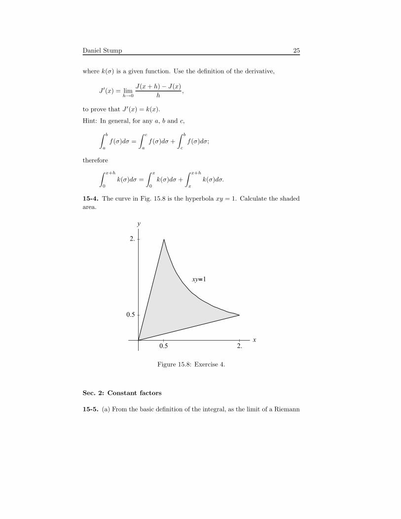
Example 4. 2 Consider a hyperbola in the first quadrant of the xy plane,

defined by the equation xy = 1; a graph of the curve is shown in Fig. 15.1.

What is the area of the region bounded above by the hyperbola, bounded

below by the x axis, and bounded on the sides by the lines x = 1 and x = 2?

The specified region is shaded in Fig. 15.1.

Solution. According to the graphical interpretation of the integral, the

area A of the specified region is equal to the integral of y(x) from x = 1 to

x = 2,

A =

∫ 2

1

y dx =

∫ 2

1

dx

x. (15-6)

1The exponential function is the only function that is its own derivative or its own

antiderivative.2This problem was considered previously in Example 3 of Chapter 12.

Daniel Stump 3

What is the antiderivative of 1/x? Recall (or find it in the Table of Deriva-

tives) that the derivative of ln x is 1/x; so the indefinite integral, or an-

tiderivative, of 1/x is∫

dx

x= ln x + C. (15-7)

Then the definite integral in (15-6) is

A = ln x|21 = ln 2− ln 1

= ln 2 ≈ 0.69315. (15-8)

The shaded area under the hyperbola in Fig. 15.1 is ln 2.

Generalizing to the domain [1, x], the area under the hyperbola from x = 1

to x is ln x. An interesting result is that the total area under the hyperbola is

infinite. Consider the domain [1, x]. As x tends to∞, the area, ln x, increases

to ∞.

Example 5. What is the total area from x = 1 to x = ∞ under the curve

in a graph of g(x) = 1/x2? The curve is shown in Fig. 15.2.

Solution. The area is

A =

∫ ∞

1

g(x)dx =

∫ ∞

1

dx

x2

=−1

x

∣∣∣∣∞

1

= 0− (−1)

= 1. (15-9)

Although the region extends to infinity, the total area is finite (A = 1). As

x increases, the height of the curve decreases rapidly so that the total area

is finite.

4 Chapter 15

15.2 HOW TO HANDLE CONSTANT FACTORS

If g(x) can be found in the right column of the Table of Derivatives in Ap-

pendix E, then∫

g(x)dx = f(x)+C where f(x) is the corresponding function

in the left column, because f ′(x) = g(x). But what about functions that are

not identical to any of the forms in the right column of the Table? If a

function g(x) is similar to one of the elementary derivatives, but differs by a

constant factor, or by a constant multiplying the variable x, then its integral

may be determined using one the following two theorems.

?

Theorem 15-1. The integral of Kg(x) where K is a constant, is

K times the integral of g(x),∫

Kg(x)dx = K

∫g(x)dx. (15-10)

In other words, if the antiderivative of g(x) is known, say f(x), then the

antiderivative of Kg(x) is also known, Kf(x).

Proof. We could prove the theorem by writing each integral in (15-10) as

the limit of a Riemann sum.3 But a much simpler proof can be based on the

fundamental theorem of calculus. Suppose an antiderivative of g(x) is f(x),

so that∫

g(x)dx = f(x) + C, (15-11)

where C is a constant of integration. The derivative of the right-hand side

of the equation is the integrand g(x) on the left; that is,

df

dx= g(x). (15-12)

Now consider the integral of Kg(x). Equation (15-10) is true if the derivative

of the right-hand side is the integrand Kg(x) on the left. But the right-hand

side of (15-10) is

K

∫g(x)dx = Kf(x) + C ′

where C ′ is a constant. (Formally, C ′ = KC; but C is an unspecified constant

of integration, so the relation between C ′ and C is irrelevant.) The derivative

3Exercise 5.

Daniel Stump 5

of this function is

d [Kf(x)]

dx= K

df

dx= Kg(x),

i.e., the integrand on the left-hand side of (15-10). Hence Theorem 15-1 is

true.

Equation (15-10) is often described by this phrase: “The constant can be

pulled out of the integral.” We’ll see below how Theorem 15-1 can be used

to calculate simple integrals. But first we’ll prove a second useful theorem.

?

Theorem 15-2. The integral of g(αx) where α is a constant, is

1/α times the integral of g(ξ) where ξ = αx,∫

g(αx)dx =1

α

∫g(ξ)dξ. (15-13)

Proof. Again we could prove the theorem by writing each integral as the

limit of a Riemann sum,3 but it is simpler to use the fundamental theorem of

calculus. Let f(x)+C be the integral of g(x), as in (15-11). Now consider the

integral of g(αx). Equation (15-13) is correct if the derivative of the function

on the right-hand side of the equation is the integrand on the left-hand side,

namely g(αx). Now, according to (15-11) the right-hand side of (15-13) is

1

α[f(ξ) + C] =

1

αf(αx) + C ′

where we have substituted ξ = αx and redefined the constant as C ′. The

derivative of this function is

d

dx

[f(αx)

α

]=

1

α

d

dxf(αx)

=1

α

[df

dξα

]by the chain rule, with ξ = αx,

=df

dξ.

But we have specified that df(x)/dx = g(x), for any value of x; therefore

df/dξ = g(ξ). Finally, then,

d

dx

[f(αx)

α

]= g(ξ) = g(αx),

which proves the theorem.

6 Chapter 15

Theorem 15-2 is an example of a change of variable. We start on the left-

hand side of (15-13) with integration over x. But the integrand is a function

of αx. So let ξ ≡ αx be a new variable. The relation of the differentials is

dξ = αdx or dx =dξ

α.

Therefore, changing the variable of integration to ξ,∫

g (αx) dx =

∫g(ξ)

dξ

α=

1

α

∫g(ξ)dξ.

In the second equality the constant 1/α has been pulled out of the integral.

As we shall see in the examples, Theorems 15-1 and 15-2 allow us to

figure out many simple integrals. If an integrand is similar to a function

with a known antiderivative, but differs by an overall constant factor K or

by a constant α multiplying the variable, then the theorems can be applied

to perform the integration. After some practice, one learns to do calculations

with (15-10) and (15-13) in his head.

15.2.1 Examples

Example 6. Determine the integral of x2.

Solution. The function x2 does not appear in the right column of the Table

of Derivatives, but 3x2 appears as the derivative of x3. If we multiply the

latter function by K = 1/3, then we have the desired function. By Theorem

15-1,∫

1

3× 3x2dx =

1

3

∫3x2dx =

1

3

(x3 + C

)

= 13x3 + C ′ (15-14)

where we have used that the integral of 3x2 is x3 + C. (The final constant of

integration C ′ is, like C, an unspecified constant.) But the integrand on the

left-hand side of (15-14) is just x2, so∫

x2dx = 13x3 + C ′. (15-15)

After determining an integral we can check the answer. Please verify that the

derivative of the right-hand side is equal to the integrand on the left-hand

side, as required.

Generalization. We can determine the integral of xp for any power p by

the same idea. The problem is to calculate∫

xpdx. Recall that the derivative

Daniel Stump 7

of xq is qxq−1. We want the derivative to be xp, so set q = p + 1,

d

dxxp+1 = (p + 1)xp. (15-16)

This differs from the specified function, xp, by the constant factor (p + 1).

So if we multiply xp+1 by Kp ≡ 1/(p + 1) then we have a function whose

derivative is xp. Thus the general formula for the integral of a power law is∫

xpdx = Kpxp+1 + C =

xp+1

p + 1+ C. (15-17)

Please show that the result in Example 5 agrees with this general formula.

A further generalization. Applying Theorem 15-1 again, for any con-

stant A,∫

Axpdx = A

∫xpdx

= A

[xp+1

p + 1+ C

]=

Axp+1

p + 1+ C ′. (15-18)

(We could just as well call the final constant of integration C instead of

C ′; it doesn’t matter what we call it because it is an unspecified constant.)

Whenever we have calculated an integral we can—and should!—double check

that it is correct. It is an easy thing to do. Just verify that the derivative of

the integral (the function on the right-hand side of the equation) equals the

integrand (the function in the integral on the left-hand side).

Example 7. Consider a graph of the function sin x. Determine the area

bounded above by the curve of sin x and below by the x axis, for 0 ≤ x ≤ π.

Figure 15.3 shows a graph of sin x with the region under the curve shaded.

In other words, the problem is to calculate the area under one hump of a sine

curve.

Solution. The area under the curve is∫ π

0 sin x dx. What is the antideriva-

tive of sin x? Look for the function sin x in the right-hand column of the

Table of Derivatives in Appendix E. Actually, sin x does not appear in the

right-hand column; but − sinx does appear as the derivative of cosx. Using

Theorem 15-1 with K = −1, we may write∫

(−) sinx dx = −∫

sin x dx. (15-19)

8 Chapter 15

Now, the left-hand side of (15-19) is cosx + C by the fundamental theorem

of calculus, because the antiderivative of − sinx is cosx. Therefore

cosx + C = −∫

sinx dx; (15-20)

or,∫

sin x dx = − cosx− C. (15-21)

(The constant of integration does not need to be designated as −C; it could

just as well be called C ′ or C, because this unspecified constant will drop

out when we calculate a definite integral.) To double check the integration,

please verify that the derivative of the integral [the right-hand side of (15-21)]

equals the integrand on the left-hand side. The sign is particularly important!

The definite integral that we need for this example is∫ π

0

sin x dx = − cosx|π0 = − cosπ − (− cos 0)

= 1 + 1 = 2. (15-22)

The final result is that the area under one hump of the sine curve is 2.

?

The next two examples make use of Theorem 15-2.

Example 8. Find the integral of e3x.

Solution. Recall that the derivative of eξ (with respect to ξ) is eξ. We seek

now the antiderivative of e3x, i.e., a function whose derivative is e3x. The

function e3x doesn’t quite work, because its derivative is 3e3x by the chain

rule. But 13e3x would work. So an antiderivative of e3x is 1

3e3x, and we may

write∫

e3xdx = 13e3x + C. (15-23)

Please verify that this equation is equivalent to (15-13) in Theorem 15-2,

with α = 3 and g(ξ) = eξ.

Generalization. What is the integral of eαx for an arbitrary constant α?

Applying Theorem 15-2, i.e., a change of variable from x to ξ ≡ αx,∫

eαxdx =1

α

∫eξdξ =

1

α

(eξ + C

)

=1

αeαx + C ′. (15-24)

Daniel Stump 9

Obviously the result (15-23) of Example 8 is just a special case of this general

formula!

Example 9. Integrate√

1 + 3.5s for s from 0 to 7.

Solution. We seek to compute∫ 7

0

√1 + 3.5s ds. The integrand, g(s) =√

1 + 3.5s, resembles√

1 + x, except that the variable s in g(s) is multiplied

by 3.5. If we can figure out the antiderivative of√

1 + x then we can apply

Theorem 15-2 to get the integral of√

1 + 3.5s.

The derivative of xp is pxp−1, and the derivative of (1+x)p is p(1+x)p−1.

We want the function whose derivative is√

1 + x, so we should take p = 3/2.

We must also multiply by 1/p to cancel the constant p from the derivative.

That is,

d

dx

2

3(1 + x)3/2 =

√1 + x. (15-25)

Now applying Theorem 15-2, the change of variable from s to x,∫ √

1 + 3.5sds =1

3.5

∫ √1 + x dx (where x = 3.5s )

=1

3.5× 2

3(1 + x)3/2 + C

=2

10.5(1 + 3.5s)

3/2+ C. (15-26)

Finally, the definite integral specified in the example is∫ 7

0

√1 + 3.5s ds =

2

10.5(1 + 3.5s)

3/2∣∣∣7

0

=2

10.5

{(25.5)3/2 − 1

}≈ 24.34. (15-27)

Generalization. As an exercise4 the same idea can be used to derive a

general formula,

∫(1 + αs)

pds =

(1 + αs)p+1

α(p + 1)+ C (15-28)

where α and p are any constants. (As a check, it is easy to show that the

derivative of the right-hand side with respect to s is the integrand on the

left-hand side.)

The exercises at the end of the chapter provide additional examples.

4Exercise 6.

10 Chapter 15

15.3 A TABLE OF INTEGRALS

It is clear from the previous section that integration of a function f(x) is

straightforward if f(x) is known as the derivative of another function F (x).

The fundamental theorem of calculus is∫

f(x) dx = F (x) + C, (15-29)

wheredF

dx= f(x). (15-30)

Also, arbitrary constant factors are easily handled. Therefore we can record

the simplest integrals in the form of a table. When one of these integrals is

needed for a calculation, we can simply look it up in the table. Appendix

F provides a short table of indefinite integrals (i.e., antiderivatives). Please

verify that the entries in the table follow simply from the basic derivatives

in Appendix E, according to (15-29) and (15-30).

In Chapter 17 we’ll study techniques of integration for calculating integrals

that are more complicated than those in Appendix F. Then we will construct

a more extensive table of integrals, given in Appendix G.

The ability to use the tables in Appendices F and G, i.e., to identify that

an integral takes one of the standard forms, is a valuable skill. But this is

not always easy! The tricky complication is that the variables in the desired

integral may differ from the variables used in the table.

Example 10. Determine the integral of sin(2πt/T ) as a function of t where

T is a constant.

Solution. The table gives∫

sin αx dx =−1

αcosαx + C. (15-31)

To convert this to the example, replace x by t and α by 2π/T . The result is∫

sin

(2πt

T

)dt = − T

2πcos

(2πt

T

)+ C. (15-32)

Example 11. Use Appendix F (and Theorems 15-1 and 15-2) to integrate

F (x) ≡ 1/(α2x2 + β2

)where α and β are arbitrary constants.

Solution. The trick to using a Table of Integrals is to recognize that∫F (x)dx resembles one of the entries in the table. In Appendix F we find

∫dx

x2 + 1= arctanx. (15-33)

Daniel Stump 11

(We’ll drop the constant of integration until the end of the calculation.) The

difference between F (x) and 1/(x2 + 1) is only the presence of the constants

α and β. Can we apply Theorems 15-1 and 15-2? At this point, art and

imagination come into the problem! We need to write the integrand in the

form

1

α2x2 + β2=

C1

(C2x)2 + 1. (C1 and C2 are constants.)

After staring at this for awhile we see that

1

α2x2 + β2=

1

β2

1

(αx/β)2 + 1.

The 1/β2 is an overall constant; pull it out of the integral (Theorem 15-1).

Then change the variable of integration to ξ ≡ α

βx, replacing dx by

dξ

(α/β)(Theorem 15-2). So,

∫dx

α2x2 + β2=

1

β2

1

α/β

∫dξ

ξ2 + 1.

The integral over ξ is the table entry (15-33), arctan ξ. Finally, then,∫

dx

α2x2 + β2=

1

αβarctan

αx

β+ C (15-34)

where C is the constant of integration.5

Computer software

Computer programs exist that can determine many integrals analytically.

Two commonly used programs are Mathematica and Maple. The user must

input a function into the program, using the format specified by the soft-

ware. Then the program returns the integral if it has a form that has been

programmed into the software. When a computer is available, this software

provides a very simple way to evaluate integrals. However, it takes practice

to develop skill in using the program. A thorough understanding of integra-

tion is necessary in order to use the software effectively. The computer makes

mathematics easier, but its use requires a good knowledge of the mathemat-

ics.

5Please verify that the answer is correct, i.e., that the derivative of the right-hand side

is the integrand on the left.

12 Chapter 15

15.4 EXAMPLES OF INTEGRATION FROM SCIENCE AND

ENGINEERING

Example 12. (from kinematics) A race car has constant acceleration

a on a drag strip. Suppose the final velocity is vf , at time tf . How far does

the car move during the time from t = 0 to t = tf? We will solve this general

problem formally, using analytic integration.

Solution. Acceleration is the rate of change of velocity, so the definition

of acceleration is a = dv/dt where v is the velocity. By the fundamental

theorem of calculus,

v(t) =

∫ t

0

a(t′)dt′. (15-35)

[Note that the derivative of the integral (the velocity) is equal to the integrand

(the acceleration).] We denote the integration variable by t′, rather than t,

because in (15-35) t stands for the endpoint of the time interval from 0 to t.

In this example a is constant. We don’t yet know its value, but whatever the

value of a the integral is∫ t

0

adt′ = at′|t0 = at− 0 = at. (15-36)

The speed is 0 at time 0, and the solution (15-36) has this initial value. At

time tf the speed is vf ; that is,

v(tf ) = atf = vf , (15-37)

which implies

a =vf

tf. (15-38)

We could have obtained this answer more easily by writing a = ∆v/∆t =

vf/tf ; however, that would only apply to constant acceleration, whereas cal-

culating the integral applies to any time dependence of a(t).

Velocity is the rate of change of distance; v = dx/dt where x is the

coordinate of the race car, i.e., the distance from the starting line. Then by

the fundamental theorem of calculus,

x(t) =

∫ t

0

v(t′)dt′. (15-39)

Daniel Stump 13

[Again, the derivative dx/dt of the integral is equal to the integrand v(t).]

Substituting the velocity function v(t′) = at′,

x(t) =

∫ t

0

at′dt′ =1

2at′2

∣∣t0

=1

2at2 − 0

= 12at2. (15-40)

The distance at time 0 is, of course 0, because the car hasn’t started moving

yet. The distance traveled at time tf is

x(tf ) =1

2

vf

tft2f = 1

2vf tf . (15-41)

Equation (15-41) is the answer to the original question: the car moves a

distance vf tf/2.

As a numerical example, suppose the race car goes from 0 to 60mph in

6 s. Then vf = 60 mi/hr = 88 ft/s and tf = 6 s. The race car moves 264 feet

during the 6 seconds of acceleration.

? ? ?

The next examples were discussed in Chap. 12, as motivation for the

importance of the integral. We are now prepared to solve them.

Example 13. (from astrophysics) Consider a simple model of the inter-

nal structure of a star, in which the density (mass per unit volume) depends

linearly on the distance from the center of the star. Figure 15.4 shows the

density ρ(r) as a function of r. The maximum density ρ0 occurs at the center

of the star, r = 0. The density decreases monotonically (and, in this simple

model, linearly) with distance from the center. At a radius R the density

is 0; this is the radius of the star. Outside radius R there is no significant

amount of matter so ρ = 0 for r ≥ R.

We’ll investigate two questions. (a) What is the total mass of the star

as a function of ρ0 and R? (b) What does the model imply for the central

density of the sun?

Part (a) Figure 15.4 shows the star subdivided into thin shells, each with

thickness ∆r. The number of shells is N = R/∆r because the total radius

R is N∆r. The total mass is the sum of the masses of the thin shells, which

we can calculate in the limit ∆r → 0.

The mass of the shell from radius r to r + ∆r is the density ρ times the

volume. The density varies slightly between r and r + ∆r, but because we’ll

take the limit ∆r → 0 the variation is negligible. That is, we can just set

ρ = ρ(r) for all points in this thin shell. The approach here is an old idea:

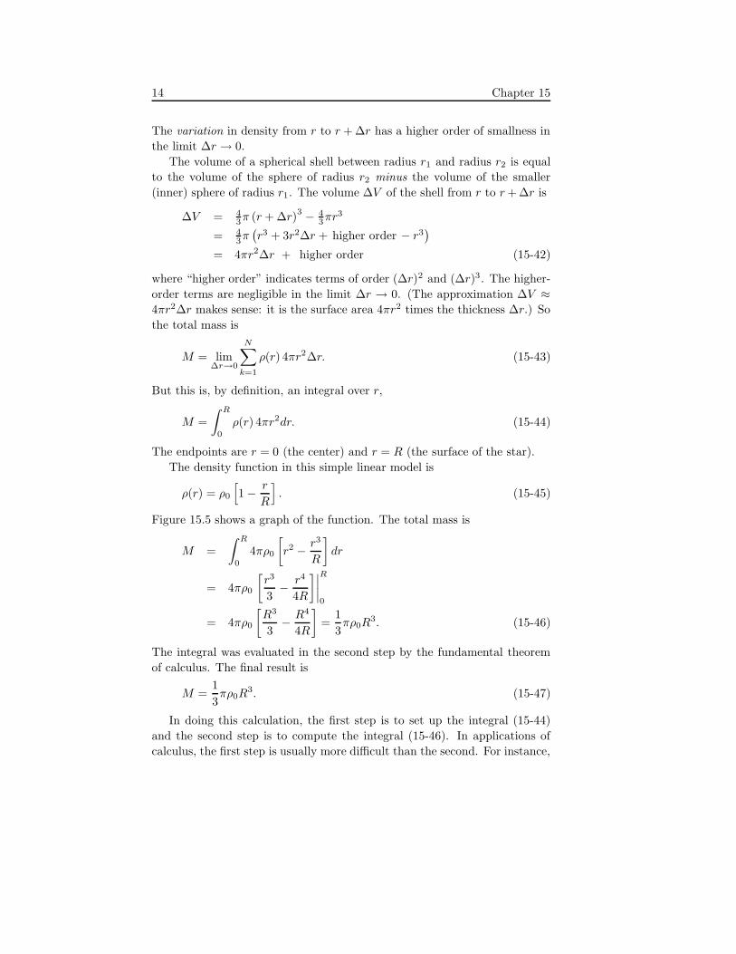
14 Chapter 15

The variation in density from r to r + ∆r has a higher order of smallness in

the limit ∆r → 0.

The volume of a spherical shell between radius r1 and radius r2 is equal

to the volume of the sphere of radius r2 minus the volume of the smaller

(inner) sphere of radius r1. The volume ∆V of the shell from r to r + ∆r is

∆V = 43π (r + ∆r)

3 − 43πr3

= 43π

(r3 + 3r2∆r + higher order − r3

)

= 4πr2∆r + higher order (15-42)

where “higher order” indicates terms of order (∆r)2 and (∆r)3. The higher-

order terms are negligible in the limit ∆r → 0. (The approximation ∆V ≈4πr2∆r makes sense: it is the surface area 4πr2 times the thickness ∆r.) So

the total mass is

M = lim∆r→0

N∑

k=1

ρ(r) 4πr2∆r. (15-43)

But this is, by definition, an integral over r,

M =

∫ R

0

ρ(r) 4πr2dr. (15-44)

The endpoints are r = 0 (the center) and r = R (the surface of the star).

The density function in this simple linear model is

ρ(r) = ρ0

[1− r

R

]. (15-45)

Figure 15.5 shows a graph of the function. The total mass is

M =

∫ R

0

4πρ0

[r2 − r3

R

]dr

= 4πρ0

[r3

3− r4

4R

]∣∣∣∣R

0

= 4πρ0

[R3

3− R4

4R

]=

1

3πρ0R

3. (15-46)

The integral was evaluated in the second step by the fundamental theorem

of calculus. The final result is

M =1

3πρ0R

3. (15-47)

In doing this calculation, the first step is to set up the integral (15-44)

and the second step is to compute the integral (15-46). In applications of

calculus, the first step is usually more difficult than the second. For instance,

Daniel Stump 15

in this example a common error would be to say that the mass is∫

ρ(r)dr.

Setting up the correct integral (15-44) is crucial.

Part (b) The mass and radius of the sun are

M = 2× 1030 kg and R = 7× 108 m. (15-48)

The simple linear model implies that the central density ρ0 is

ρ0 =3M

πR3=

3× 2× 1030 kg

π (7× 108 m)3 = 5.6× 103 kg/m

3. (15-49)

For comparison, the density of liquid water is 1× 103 kg/m3.

Example 14. (from mechanical engineering) A massive flywheel may

be used to store kinetic energy. How much kinetic energy is present in a

rotating disk with mass M = 450kg, radius R = 0.6m, and height h = 0.1m,

if the period of rotation is T = 0.1 s?

Solution. Figure 15.6 shows the cylindrical flywheel. In the figure, the

flywheel is subdivided into N small cylindrical shells of thickness ∆r. The

total radius is R = N∆r so the number of shells is N = R/∆r. The total

kinetic energy is the sum of the kinetic energies of the elemental shells. To

calculate this total we’ll calculate the sum in the limit ∆r → 0.

The kinetic energy ∆K of the shell from r to r + ∆r is 12 (∆m)v2 where

∆m is the mass of the shell and v is the speed of points in this shell. The

mass is ∆m = ρ∆V where ρ is the mass density of the material,

ρ =M

V=

M

πR2h, (15-50)

and ∆V is the volume of the shell,

∆V =[π (r + ∆r)

2 − πr2]h

= 2πrh∆r + higher order (15-51)

where “higher order” means terms of order (∆r)2, which will be negligible in

the limit ∆r → 0. (The approximation ∆V ≈ 2πrh∆r makes sense: it is the

surface area 2πrh of the thin cylindrical shell times the thickness ∆r.)

The speed of a point in the flywheel depends on the radius r. The point

at the center has 0 speed. The points on the outer rim have the greatest

speed. A point at radius r travels a distance 2πr in each revolution, i.e., in

the time T (= the period of revolution); therefore the speed as a function of

r is

v(r) =2πr

T. (15-52)

16 Chapter 15

The period of revolution is, of course, the same for all points. The speed of

a point in the flywheel is proportional to the distance from the center.

Combining these results, the total kinetic energy is

K = lim∆r→0

N∑

k=1

1

2ρ (2πrkh∆r)

(2πrk

T

)2

= lim∆r→0

N∑

k=1

4π3ρh

T 2r3k∆r. (15-53)

By definition the limit of the sum is an integral,

K =

∫ R

0

4π3ρh

T 2r3dr. (15-54)

This is evaluated by the fundamental theorem of calculus,

K =4π3ρh

T 2

r4

4

∣∣∣∣R

0

=π3ρhR4

T 2. (15-55)

We may rewrite the result in terms of the mass M by replacing ρ by the

expression in (15-50). After some algebraic simplification the final result is

K =π2MR2

T 2(15-56)

For the parameters specified in the example, the total kinetic energy is6

K =π2(450 kg)(0.6 m)2

(0.1 s)2= 1.6× 105 J. (15-57)

Moment of Inertia. In mechanical engineering the moment of inertia

I of a rotating object is an important parameter. In general, the kinetic

energy is 12Iω2 where ω = 2π/T is the angular velocity. Comparing 1

2Iω2 to

the formula (15-56) for a rotating solid cylinder, we see that the moment of

inertia of the flywheel is

I = 12MR2. (15-58)

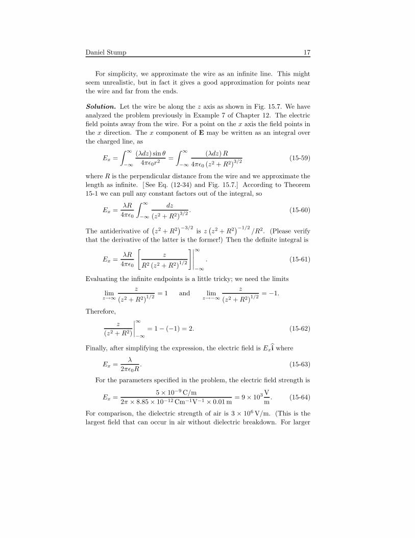
Example 15. (from electrostatics) A standard problem in electrostatics

is to calculate the electric field and potential due to a given distribution

of electric charge. For example, suppose a long wire has charge density

λ = 5 × 10−9 C/m. What is the strength of the electric field at a distance

R = 1 cm from the wire?

6The joule (J) is a unit of energy defined by 1 J = 1 kg m2/s2.

Daniel Stump 17

For simplicity, we approximate the wire as an infinite line. This might

seem unrealistic, but in fact it gives a good approximation for points near

the wire and far from the ends.

Solution. Let the wire be along the z axis as shown in Fig. 15.7. We have

analyzed the problem previously in Example 7 of Chapter 12. The electric

field points away from the wire. For a point on the x axis the field points in

the x direction. The x component of E may be written as an integral over

the charged line, as

Ex =

∫ ∞

−∞

(λdz) sin θ

4πε0r2=

∫ ∞

−∞

(λdz) R

4πε0 (z2 + R2)3/2

(15-59)

where R is the perpendicular distance from the wire and we approximate the

length as infinite. [ See Eq. (12-34) and Fig. 15.7.] According to Theorem

15-1 we can pull any constant factors out of the integral, so

Ex =λR

4πε0

∫ ∞

−∞

dz

(z2 + R2)3/2

. (15-60)

The antiderivative of(z2 + R2

)−3/2is z

(z2 + R2

)−1/2/R2. (Please verify

that the derivative of the latter is the former!) Then the definite integral is

Ex =λR

4πε0

[z

R2 (z2 + R2)1/2

]∣∣∣∣∣

∞

−∞

. (15-61)

Evaluating the infinite endpoints is a little tricky; we need the limits

limz→∞

z

(z2 + R2)1/2

= 1 and limz→−∞

z

(z2 + R2)1/2

= −1.

Therefore,

z

(z2 + R2)

∣∣∣∣∞

−∞

= 1− (−1) = 2. (15-62)

Finally, after simplifying the expression, the electric field is Ex i where

Ex =λ

2πε0R. (15-63)

For the parameters specified in the problem, the electric field strength is

Ex =5× 10−9 C/m

2π × 8.85× 10−12 Cm−1V−1 × 0.01 m= 9× 103 V

m. (15-64)

For comparison, the dielectric strength of air is 3 × 106 V/m. (This is the

largest field that can occur in air without dielectric breakdown. For larger

18 Chapter 15

fields the molecules are ionized, the air is a plasma, and current flows.)

Example 14 is rather advanced for an introduction to calculus, because it

involves a vectorial quantity—the electric field. However, it is a good example

to show how integration is applied to problems in field theory.

Example 16. (from probability and statistics) Consider an experi-

ment in which some quantity u is measured many times. The mean value is

u and the standard deviation (= root mean square fluctuation) is σ. What is

the probability that a single measurement will lie between u− σ and u + σ?

Solution. The normal (or, Gaussian) distribution of measurement errors is

P (u) =1√

2πσ2exp

[− (u− u)

2/2σ2

]. (15-65)

P (u)du is the probability that a measurement of the quantity would be be-

tween u and u + du. The expected measurement (= mean of many measure-

ments) is∫ ∞

−∞uP (u)du = u,

and the mean square fluctuation is∫ ∞

−∞(u− u)2 P (u)du = σ2.

The probability that a measurement will be between u − σ and u + σ, i.e.,

within one standard deviation of the mean, is

P1 =

∫ u+σ

u−σ

e−(u−u)2/2σ2 du√2πσ2

=

∫ σ

−σ

e−ξ2/2σ2 dξ√2πσ2

; (15-66)

in the second line the variable has been changed from u (the measurement)

to ξ ≡ u− u (the fluctuation). Using Theorems 15-1 and 15-2 to handle the

constants,

P1 =1√2π

∫ 1

−1

e−x2/2dx (15-67)

where x = ξ/σ. Finally, the integral can be computed by expanding the

exponential in a power series,

∫ 1

−1

e−x2/2dx =

∫ 1

−1

∞∑

n=0

(−1)n

n!

(x2

2

)n

dx

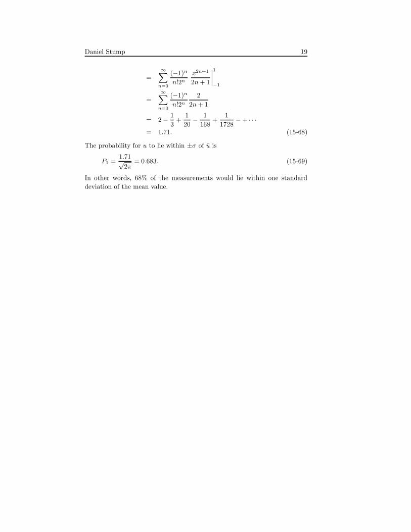
Daniel Stump 19

=∞∑

n=0

(−1)n

n!2n

x2n+1

2n + 1

∣∣∣∣1

−1

=

∞∑

n=0

(−1)n

n!2n

2

2n + 1

= 2− 1

3+

1

20− 1

168+

1

1728−+ · · ·

= 1.71. (15-68)

The probability for u to lie within ±σ of u is

P1 =1.71√

2π= 0.683. (15-69)

In other words, 68% of the measurements would lie within one standard

deviation of the mean value.

Figure 15.1: Example 4. What is the area of the shaded region under the

hyperbola?

20

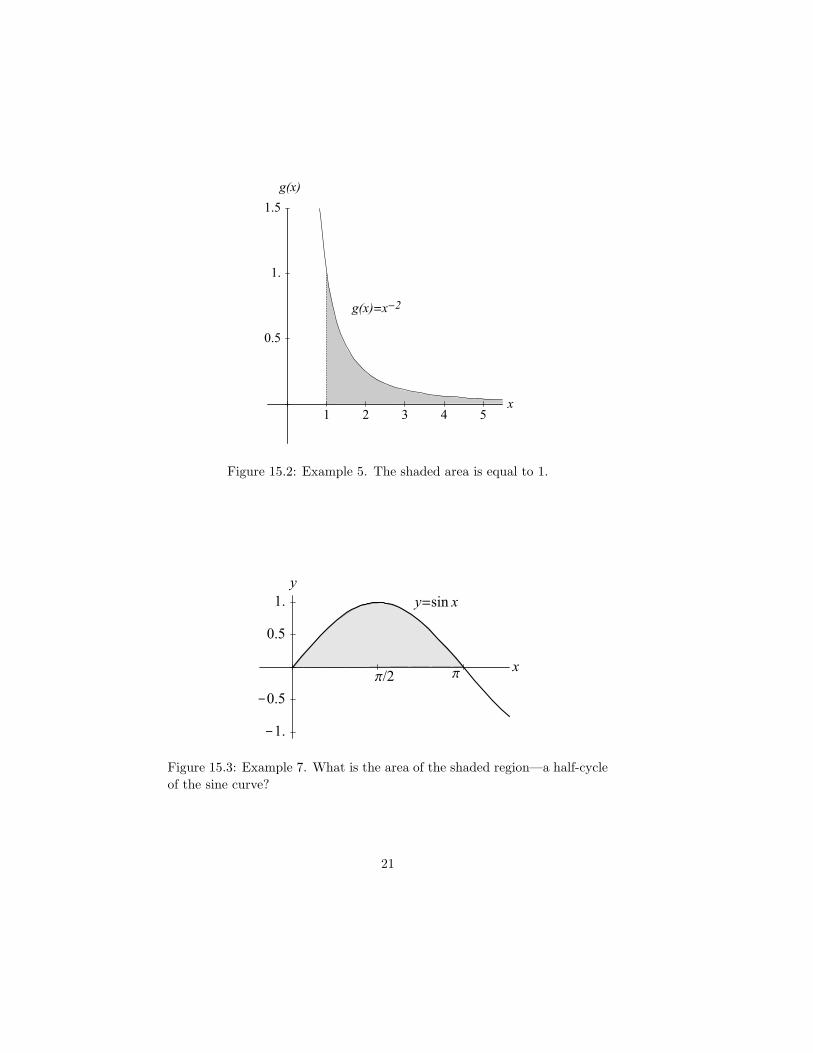
Figure 15.2: Example 5. The shaded area is equal to 1.

Figure 15.3: Example 7. What is the area of the shaded region—a half-cycle

of the sine curve?

21

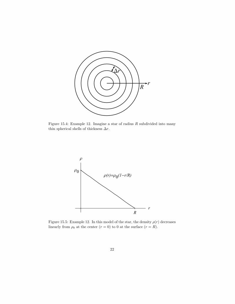
Figure 15.4: Example 12. Imagine a star of radius R subdivided into many

thin spherical shells of thickness ∆r.

Figure 15.5: Example 12. In this model of the star, the density ρ(r) decreases

linearly from ρ0 at the center (r = 0) to 0 at the surface (r = R).

22

Figure 15.6: Example 13. A rotating flywheel of radius R and height h. To

calculate the total kinetic energy, the wheel is subdivided into cylindrical

shells of thickness ∆r. The speed of a point on the wheel is proportional to

the distance r from the center.

Figure 15.7: Example 14. A charged wire. ∆E is the contribution to the

electric field from the small charge element ∆q = λ∆z. The overall field at

P is iEx in (15-59).

23

24 Chapter 15

EXERCISES

Sec. 1: Introduction

15-1. For each function f(x) determine the total area under the curve in a

graph of f(x) for the specified domain [a, b]. Sketch a graph of the function,

estimate the area by geometrical methods (try to be accurate!) and compare

your estimate to the exact calculated area.

(a) f(x) = e−x for a = 0 and b = ∞.

(b) f(x) = (1 + x)−1 for a = 0 and b = 10.

(c) f(x) = 6x for a = 0 and b = 10.

(d) f(x) = 1 + 5x2 for a = −1 and b = 1.

(e) f(x) = (1 + x2)−1 for a = −∞ and b = ∞. [Hint: look up the derivative

of arctanx.] Although the graph of (1+x2)−1 has no resemblance to a circle,

the area under the curve is π.

15-2. The equation for a semicircle of radius 1 is y = f(x) where f(x) =√1− x2.

(a) Sketch a graph of the function and shade the region bounded by the

curve. (What is the area of the shaded region?)

(b) Prove that the antiderivative of f(x) is

Φ(x) = 12

[arcsinx + x

√1− x2

].

That is, prove Φ′(x) = f(x).

(c) Calculate the area of the shaded region of (a) by integration,

area =

∫ 1

−1

f(x)dx.

(d) Explain how these results imply that the area of a circle is πr2.

15-3. Define a function J(x) by

J(x) =

∫ x

0

k(σ)dσ.

Daniel Stump 25

where k(σ) is a given function. Use the definition of the derivative,

J ′(x) = limh→0

J(x + h)− J(x)

h,

to prove that J ′(x) = k(x).

Hint: In general, for any a, b and c,

∫ b

a

f(σ)dσ =

∫ c

a

f(σ)dσ +

∫ b

c

f(σ)dσ;

therefore

∫ x+h

0

k(σ)dσ =

∫ x

0

k(σ)dσ +

∫ x+h

x

k(σ)dσ.

15-4. The curve in Fig. 15.8 is the hyperbola xy = 1. Calculate the shaded

area.

Figure 15.8: Exercise 4.

Sec. 2: Constant factors

15-5. (a) From the basic definition of the integral, as the limit of a Riemann

26 Chapter 15

sum [see Eq. (13-4)], prove Theorem 15-1.

(b) Similarly, prove Theorem 15-2. (Hint: Let ξ = αx. Draw a picture

showing the x axis and, below it, the ξ axis. The integration region on the x

axis is some interval [a, b] which corresponds to an interval [αa, αb] on the ξ

axis. The subdivision of the x domain corresponds to a subdivision of the ξ

domain.)

15-6. Derive this general integral formula:

∫(1 + αs)

pds =

(1 + αs)p+1

α (p + 1)+ C.

15-7. Use Theorem 15-2 to prove

1

a

∫ a

0

g(x

a

)dx =

∫ 1

0

g(x)dx

for any function g(x).

15-8. Evaluate these definite or indefinite integrals using Theorems 15-1 and

15-2 to handle the constant factors. In each case, begin by identifying the

integral with one of the standard forms in Appendix F, perhaps modified by

constant factors.

(a)

∫ 1

0

5

x2 + 1dx (b)

∫ 1

0

5

x2 + 2dx. Hint: Let ξ =

√2x.

(c)

∫ ∞

0

e−udu. Hint: Let ξ = −u. (d)

∫ ∞

0

e−t/T dt. Hint: Let ξ = −t/T .

(e)

∫ (ax2 + bx + c

)dx (f)

∫ 7

0

(ax2 + bx + c

)dx

(g)

∫dx

1− x2(h)

∫dx

1− 3x2

Sec. 3: A Table of Integrals

15-9. Look up the antiderivatives for these functions in the Table of Inte-

grals in Appendix F. Where necessary use Theorems 15-1 and 15-2 to handle

constant factors. In each case, begin by identifying the integral with one

of the standard forms in Appendix F, perhaps modified by constant factors.

For extra credit, check the answers using Mathematica or Maple.

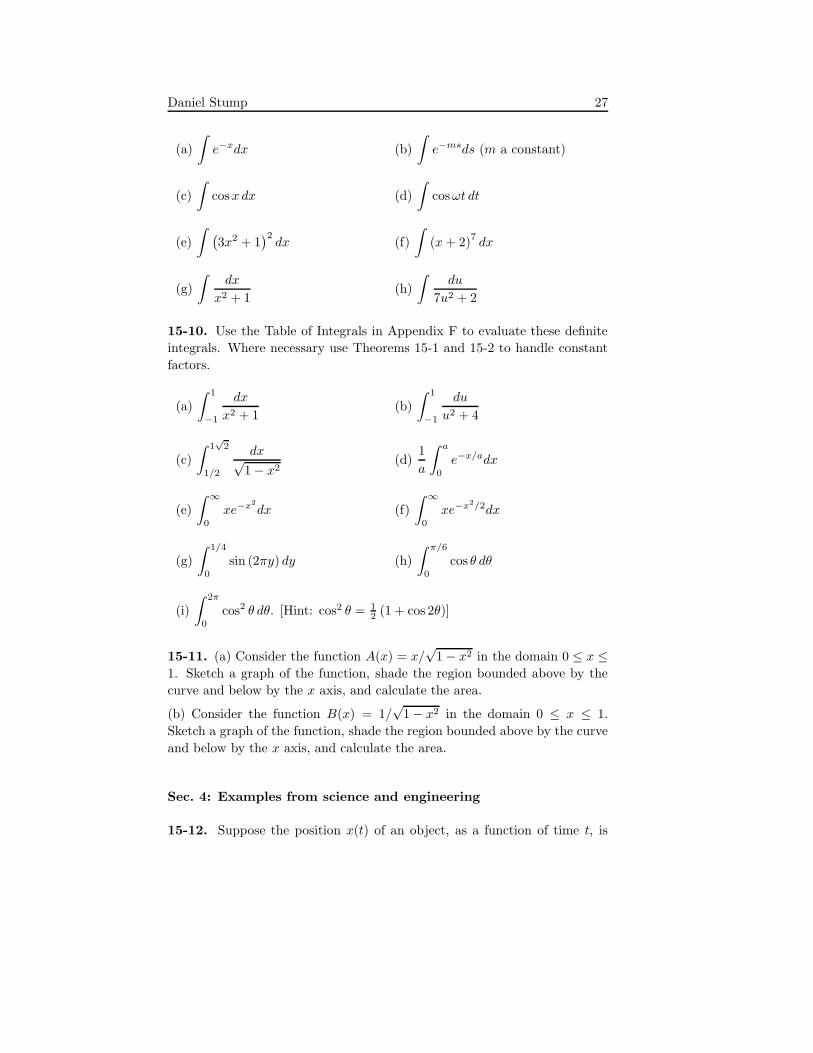
Daniel Stump 27

(a)

∫e−xdx (b)

∫e−msds (m a constant)

(c)

∫cosx dx (d)

∫cosωt dt

(e)

∫ (3x2 + 1

)2dx (f)

∫(x + 2)

7dx

(g)

∫dx

x2 + 1(h)

∫du

7u2 + 2

15-10. Use the Table of Integrals in Appendix F to evaluate these definite

integrals. Where necessary use Theorems 15-1 and 15-2 to handle constant

factors.

(a)

∫ 1

−1

dx

x2 + 1(b)

∫ 1

−1

du

u2 + 4

(c)

∫ 1√

2

1/2

dx√1− x2

(d)1

a

∫ a

0

e−x/adx

(e)

∫ ∞

0

xe−x2

dx (f)

∫ ∞

0

xe−x2/2dx

(g)

∫ 1/4

0

sin (2πy) dy (h)

∫ π/6

0

cos θ dθ

(i)

∫ 2π

0

cos2 θ dθ. [Hint: cos2 θ = 12 (1 + cos 2θ)]

15-11. (a) Consider the function A(x) = x/√

1− x2 in the domain 0 ≤ x ≤1. Sketch a graph of the function, shade the region bounded above by the

curve and below by the x axis, and calculate the area.

(b) Consider the function B(x) = 1/√

1− x2 in the domain 0 ≤ x ≤ 1.

Sketch a graph of the function, shade the region bounded above by the curve

and below by the x axis, and calculate the area.

Sec. 4: Examples from science and engineering

15-12. Suppose the position x(t) of an object, as a function of time t, is

28 Chapter 15

given by an integral

x(t) =

∫ t

0

w(t′)dt′.

(a) Show that x(t+∆t)−x(t) ≈ w(t)∆t for small ∆t. (Hint: Use the integral

identity∫ b

a=

∫ c

a+

∫ b

c.)

(b) From (a) prove that dx/dt = w(t), i.e., w(t) is the velocity.

15-13. Each part of this exercise gives a velocity function v(t) for a moving

object. Determine the position (i.e., coordinate) x(t) as a function of time.

(Assume x(0) = 0.) In each case sketch graphs of v(t) and x(t) versus t.

(a) v(t) = 5m/s (b) v(t) = v0 + Ct (v0 and C constants)

(c) v(t) = t2(3− t)2 for 0 ≤ t ≤ 3 (d) v(t) = A sin ωt (A and ω constants)

(e) v(t) = 3e−0.2t (f) v(t) =6t√

t2 + 4

15-14. Each part of this exercise gives a velocity function v(t) for a moving

object. Determine the total displacement for the specified time interval,

[t1, t2]. In some cases usits are given and in others the units are left arbitrary.

(a) v(t) = 5m/s for [0, 6 s] (b) v(t) = 10 ft/s− (32 ft/s2)t for [0, 2 s]

(c) v(t) = t2(3− t)2 for [0, 3] (d) v(t) = A sin ωt for [0, 2π/ω]

(e) v(t) = 3e−0.2t for [0,∞] (f) v(t) =6t√

t2 + 4for [0, 3]

15-15. The moment of inertia I of a body about an axis of rotation is defined

by

I =

∫

body

r2dm

where dm = mass element in the body and r = perpendicular distance from

dm to the axis of rotation. Consider a right circular cylinder (mass M ,

radius R, and height h). Derive the formula for I about the cylinder axis.

The method is to subdivide the cylinder into cylindrical shells (the elements)

of width dr and to add their contributions to I . Note that dm = ρ dV where

Daniel Stump 29

ρ = M/V = density, and dV = volume of the elemental shell.

15-16. (a) Derive a formula for the moment of inertia of a sphere (mass

M and radius a) about an axis through the center of the sphere. (Hint:

Subdivide the sphere into elemental disks as shown in Fig. 15.9. The moment

of inertia of an elemental disk is dI = 12 (dm) r2 where r = radius, dm =

mass = ρπr2dz and ρ = density. )

(b) A cylinder and a sphere, of equal radius R and mass M , roll down an

inclined plane, starting from rest at the same height. Explain why the sphere

rolls faster.

Figure 15.9: Exercise 16. To calculate the moment of inertia of a sphere,

subdivide the sphere into elemental disks. The radius of an elemental disk is

r =√

a2 − z2 and the thickness is dz.

15-17. A wire of length L is uniformly charged with total charge Q (charge

per unit length λ = Q/L). Determine the electric field on the midplane of

the wire as a function of perpendicular distance r from the wire. (Hint: Let

the wire lie on the z axis from −L/2 to L/2. Detemine the field Ex(x) for

points on the x axis.) Show that E(r) behaves as r−1 for r � L, and as r−2

for r � L.

30 Chapter 15

General Exercises

15-18. Consider a set of small masses mi occupying points (xi, yi) in the xy

plane. (The index i = 1, 2, 3, . . . , N labels the masses.) The center of mass

point (xc, yc) is the “average point” weighted by the masses,

xc =

∑Ni=1 mixi∑Ni=1 mi

and yc =

∑Ni=1 miyi∑Ni=1 mi

.

Similarly, for a continuous distribution of mass, i.e., a flat plate in the xy

plane, the coordinates of the center of mass point are

xc =1

M

∫x dm and yc =

1

M

∫y dm

where dm denotes a mass element and M =∫

dm is the total mass. Find the

center of mass point of a flat plate in the shape of a right isoceles triangle.

(Hint: Set up a coordinate system with the hypotenuse of the triangle on the

x axis. Subdivide the plate into elemental strips parallel to the x axis.)

15-19. Work and potential energy. The elastic force on a mass m is

F (x) = −kx (Hooke’s law)

where k is the spring constant. The mass moves on the x axis. A positive

force is toward the right, i.e., toward increasing x.

(a) Show that x = 0 is a stable equilibrium point: for either x > 0 or x < 0

the force pulls toward x = 0.

(b) The work W done by the force as m moves from x = a to x = b is defined

by W =∫ b

aF (x)dx. Calculate the work done if m moves from x = a to

x = 0.

(c) The potential energy U(x) as a function of the position x of m is defined

as the work done by the force if m moves from position x to the equilibrium

position. Determine U(x).

(d) Prove that F (x) = −U ′(x).

15-20. A mathematical farmer has decided that his potato patch should

be bounded by a square-root curve, because the potato is a root vegetable.

His field has dimensions 100 ft× 100 ft, and the potato patch is shown in Fig.

15.10. What is the area of the potato patch?

Daniel Stump 31

Figure 15.10: Exercise 20. A potato patch bounded by a square root curve,

y = 10√

x.

15-21. Sketch the unit circle in the xy plane centered at the origin; the

equation for the circle is x2 + y2 = 1. Sketch a vertical line at x = 1/2.

The region inside the circle with x > 1/2 is called a chord of the circle.

What is the area of this chord? Determine the answer in two ways: (i) by

integration, and (ii) by regarding the chord as the circular segment minus a

triangle. [Answer: π/3−√

3/4]

32 Chapter 15

Contents

15.1 Introduction . . . . . . . . . . . . . . . . . . . . . . . . . . . . 1

15.2 How to handle constant factors . . . . . . . . . . . . . . . . . 4

15.2.1 Examples . . . . . . . . . . . . . . . . . . . . . . . . . 6

15.3 A Table of Integrals . . . . . . . . . . . . . . . . . . . . . . . 10

15.4 Examples of integration from science and engineering . . . . . 12