15. Business Process Analysis and Simulationdisi.unitn.it/~dalpiaz/ois/lib/exe/fetch.php?media=15-bpanalysis.pdf · Business Process Analysis and Simulation ... Generating non-standard

© F. Dalpiaz & J. Mylopoulos -- OIS 2011-12 Slide 1

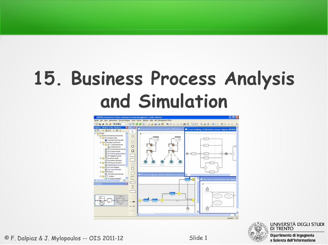
15. Business Process Analysis and Simulation


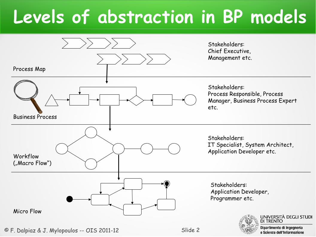
Levels of abstraction in BP models

Process Map

Business Process

Workflow(„Macro Flow“)

Micro Flow

Stakeholders:Chief Executive,Management etc.

Stakeholders:Process Responsible, Process Manager, Business Process Expert etc.

Stakeholders:IT Specialist, System Architect,Application Developer etc.

Stakeholders:Application Developer,Programmer etc.


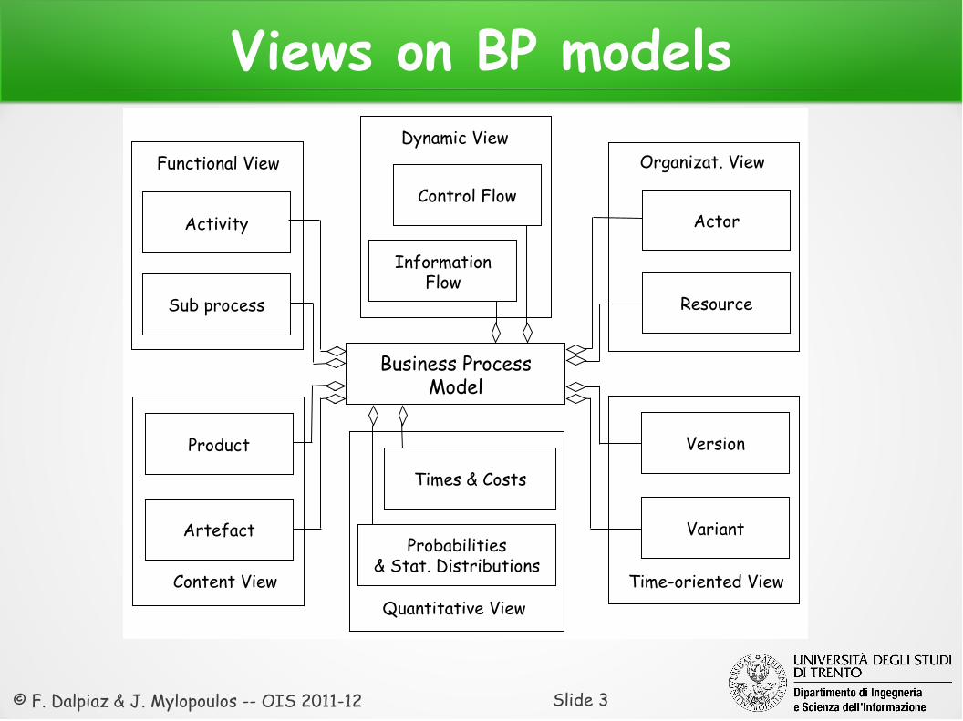
Views on BP modelsDynamic View

Content View

Organizat. ViewFunctional View

Time-oriented ViewQuantitative View

Business ProcessModel

InformationFlow

Control Flow

Times & Costs

Probabilities& Stat. Distributions

Product

Artefact

Sub process

Activity

Version

Variant

Actor

Resource


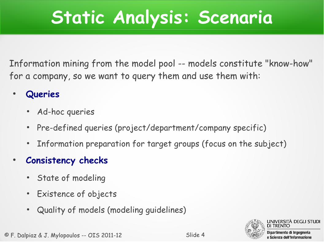
Static Analysis: Scenaria

Information mining from the model pool -- models constitute "know-how" for a company, so we want to query them and use them with:

● Queries● Ad-hoc queries● Pre-defined queries (project/department/company specific)● Information preparation for target groups (focus on the subject)

● Consistency checks● State of modeling● Existence of objects● Quality of models (modeling guidelines)


Static Analysis: Scenaria

● Evaluation of simulation results● Generating non-standard simulation results, e.g., "Determine all

processes which have a cycle time greater than 5 days“● Connecting static and dynamic model information, e.g., "Determine

activities that occur in processes with cycle time >5 days")


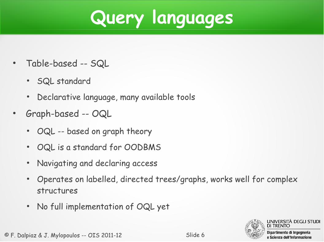
Query languages

● Table-based -- SQL ● SQL standard ● Declarative language, many available tools

● Graph-based -- OQL ● OQL -- based on graph theory● OQL is a standard for OODBMS ● Navigating and declaring access● Operates on labelled, directed trees/graphs, works well for complex

structures● No full implementation of OQL yet


Query languages

● Query-by-Example● Dialog- or editor-supported● No standard, tool-dependent (but some common features...) ● Queries formulated through powerful front-end● User needs no knowledge of the actual query language


Granularity of queries

● Attribute Level● Query on object properties● "Give me the execution time of activity ‘risk check’ "

● Object/Class level● Number of objects that satisfy a property● "Find all activities with execution time > 1h."● "Find all instances of class document. "


Granularity of queries

● Model level● Explore one or a few models● "Which activities are needed for processing a credit application?"

● System Level● Queries over all the models● "Find all business processes that require manual activity."


Information aggregation

● Table-oriented● View query results in table-oriented form● Most users are familiar with this representation (Excel spreadsheets)

● Graphical● Good representation of quantity-oriented results (pie charts, bar charts) ● Intuitive representation of different result sets

● Relation-/Dependency Graph● Representation of dependencies in query result● Visualization of complex model structures (Part-of, model dependencies)● Generation of model-spanning views (process hierarchies, role-activity-

diagrams)


ADONIS Query Language (AQL)

● The ADONIS Query Language (AQL) is an adaptation of OQL● In ADONIS, you can choose a query from a library of queries, or

define your own using AQL


AQL Examples (1)

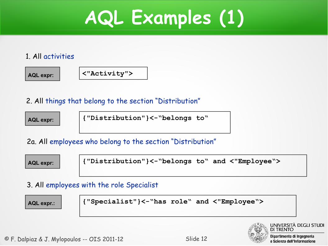
1. All activities

AQL expr: <"Activity">

2. All things that belong to the section “Distribution”

AQL expr: {"Distribution"}<-“belongs to“

3. All employees with the role Specialist

AQL expr.: {"Specialist"}<-“has role“ and <"Employee“>

AQL expr: {"Distribution"}<-“belongs to“ and <"Employee“>

2a. All employees who belong to the section “Distribution”


AQL Examples (2)

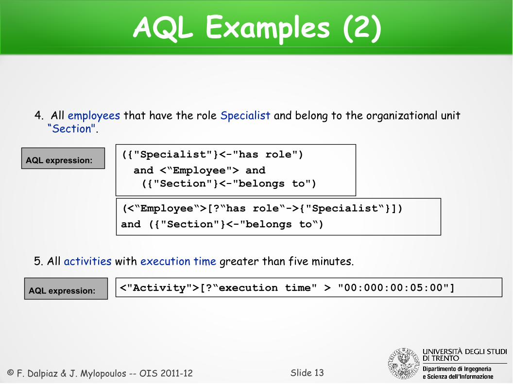
<"Activity">[?“execution time" > "00:000:00:05:00"]

4. All employees that have the role Specialist and belong to the organizational unit “Section".

AQL expression:({"Specialist"}<-"has role")

and <“Employee"> and ({"Section"}<-"belongs to")

AQL expression:

5. All activities with execution time greater than five minutes.

(<“Employee“>[?“has role“->{"Specialist“}])

and ({"Section"}<-"belongs to“)


Predefined Queries

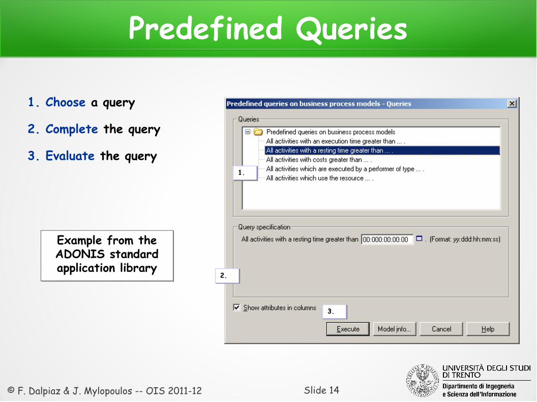
1. Choose a query

2. Complete the query

3. Evaluate the query

Example from theADONIS standard application library

Example from theADONIS standard application library

3.3.

2.2.

1.1.


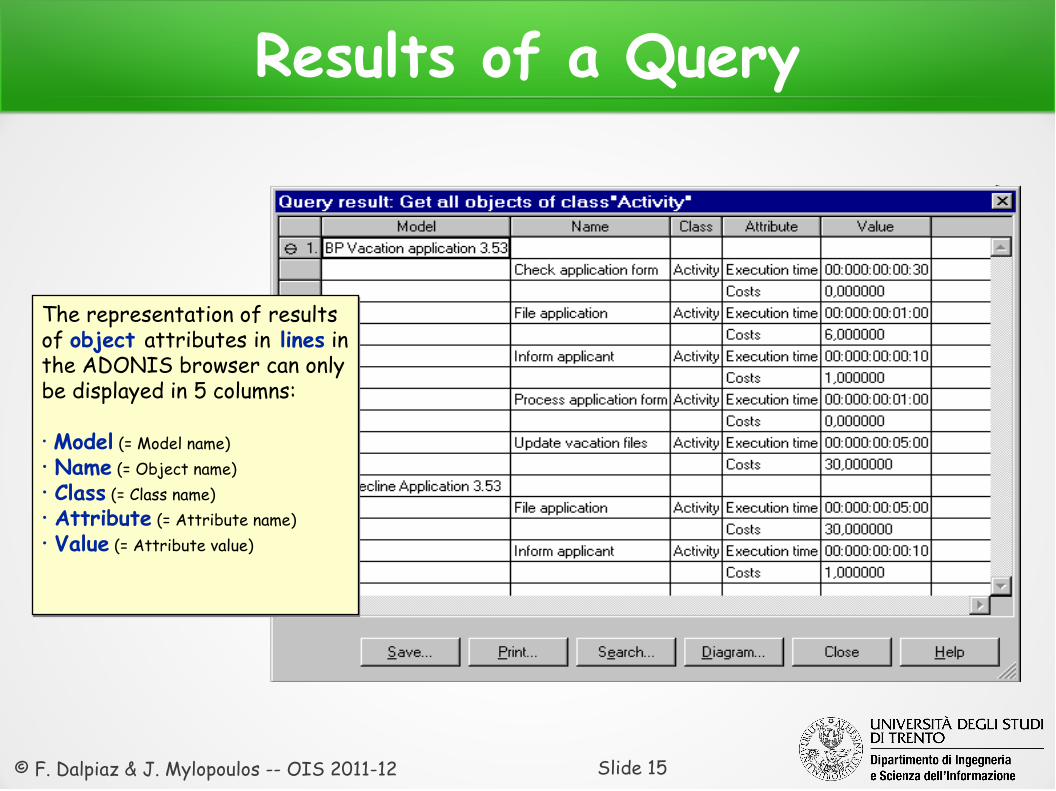
Results of a Query

The representation of results of object attributes in lines in the ADONIS browser can only be displayed in 5 columns:

• Model (= Model name)• Name (= Object name)• Class (= Class name)• Attribute (= Attribute name)• Value (= Attribute value)

The representation of results of object attributes in lines in the ADONIS browser can only be displayed in 5 columns:

• Model (= Model name)• Name (= Object name)• Class (= Class name)• Attribute (= Attribute name)• Value (= Attribute value)


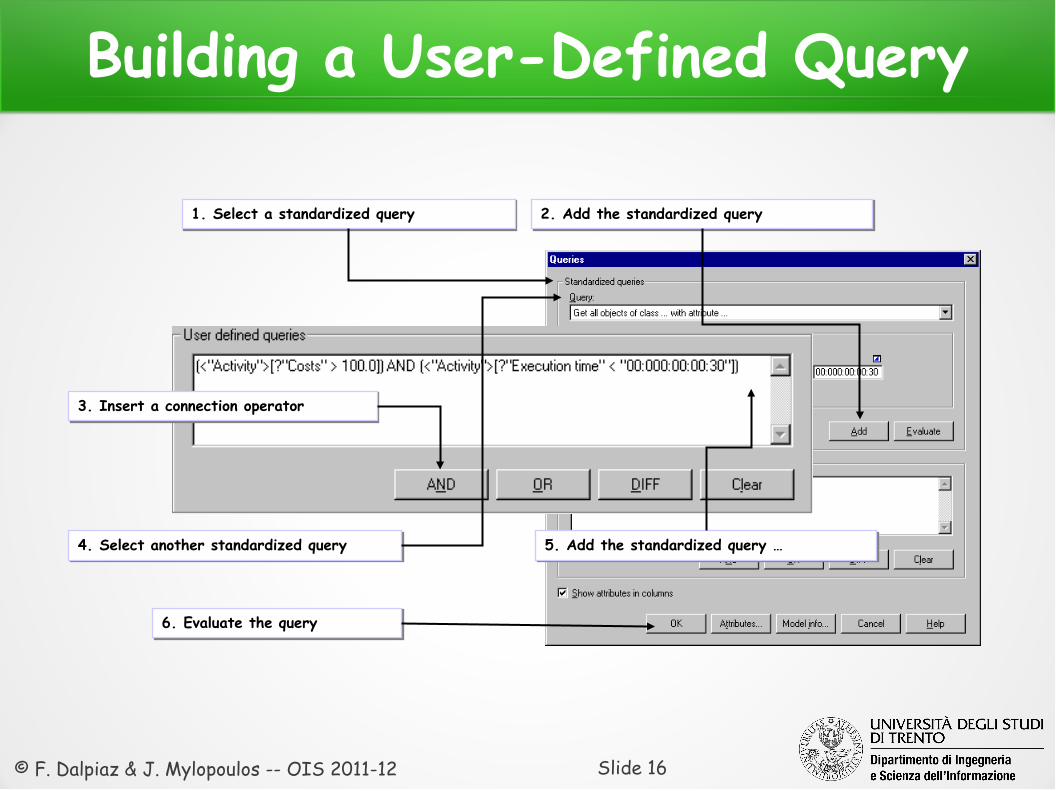
Building a User-Defined Query

6. Evaluate the query 6. Evaluate the query

3. Insert a connection operator3. Insert a connection operator

2. Add the standardized query2. Add the standardized query1. Select a standardized query1. Select a standardized query

5. Add the standardized query …5. Add the standardized query …4. Select another standardized query4. Select another standardized query


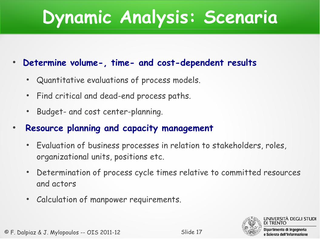
Dynamic Analysis: Scenaria

● Determine volume-, time- and cost-dependent results ● Quantitative evaluations of process models.● Find critical and dead-end process paths.● Budget- and cost center-planning.

● Resource planning and capacity management● Evaluation of business processes in relation to stakeholders, roles,

organizational units, positions etc. ● Determination of process cycle times relative to committed resources

and actors● Calculation of manpower requirements.


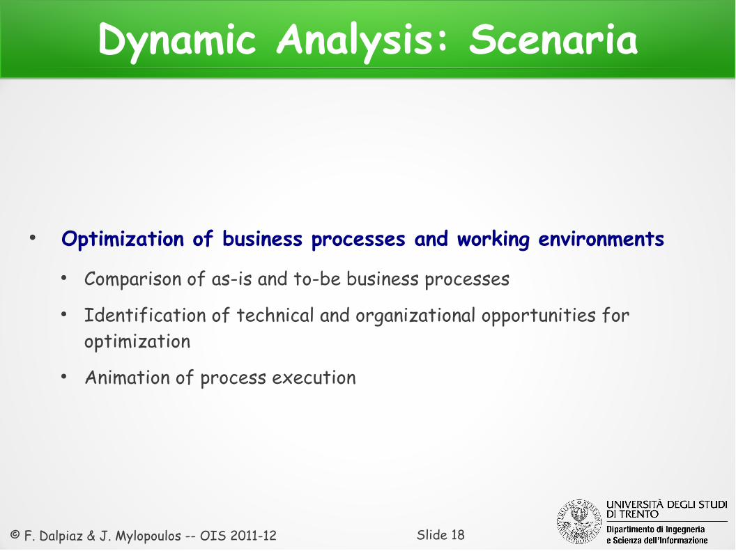
Dynamic Analysis: Scenaria

● Optimization of business processes and working environments● Comparison of as-is and to-be business processes● Identification of technical and organizational opportunities for

optimization● Animation of process execution


What are we measuring?

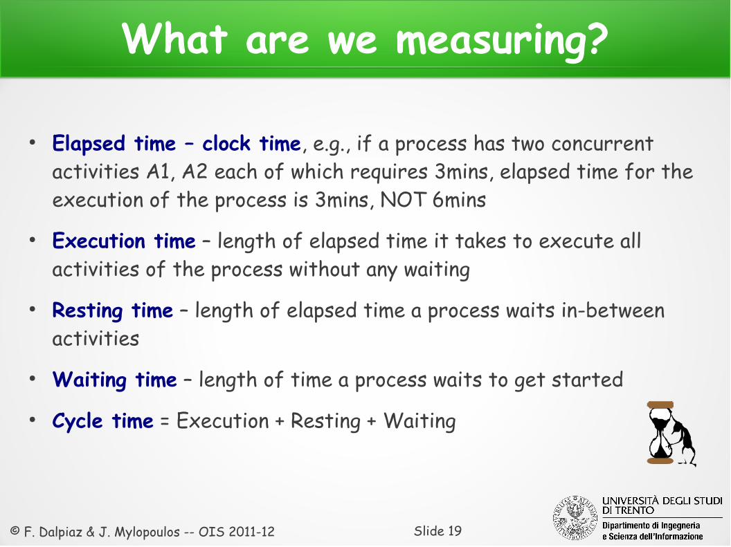
● Elapsed time – clock time, e.g., if a process has two concurrent activities A1, A2 each of which requires 3mins, elapsed time for the execution of the process is 3mins, NOT 6mins

● Execution time – length of elapsed time it takes to execute all activities of the process without any waiting

● Resting time – length of elapsed time a process waits in-between activities

● Waiting time – length of time a process waits to get started● Cycle time = Execution + Resting + Waiting


Approximate Dynamic Analysis: Pros● Process structure need not be acquired

● The acquisition of activity sequences and the control flow is not needed● Existing information, such as activity lists, serve as input for evaluation

and analysis ("smooth transition")

● Capacity analysis● Despite small acquisition effort, necessary capacity can be determined● Analysis can be conducted with standard software (e.g., Excel)

● Analysis can be done manually, or with simple software tools● Quantitative data as basis for further analysis● If the process model is enriched with control structures, existing data

can be re-used


Approximate Dynamic Analysis: Cons

● Process cycle time (execution time + waiting time) can't be calculated● Because of missing process structures

● Activity dependencies are not considered● Dependencies in the control flow of the business processes as well as

cycles or concurrency are not considered in the evaluation

● No dynamic resource planning● Resource and capacity planning based on dynamically calculated waiting

times is not possible


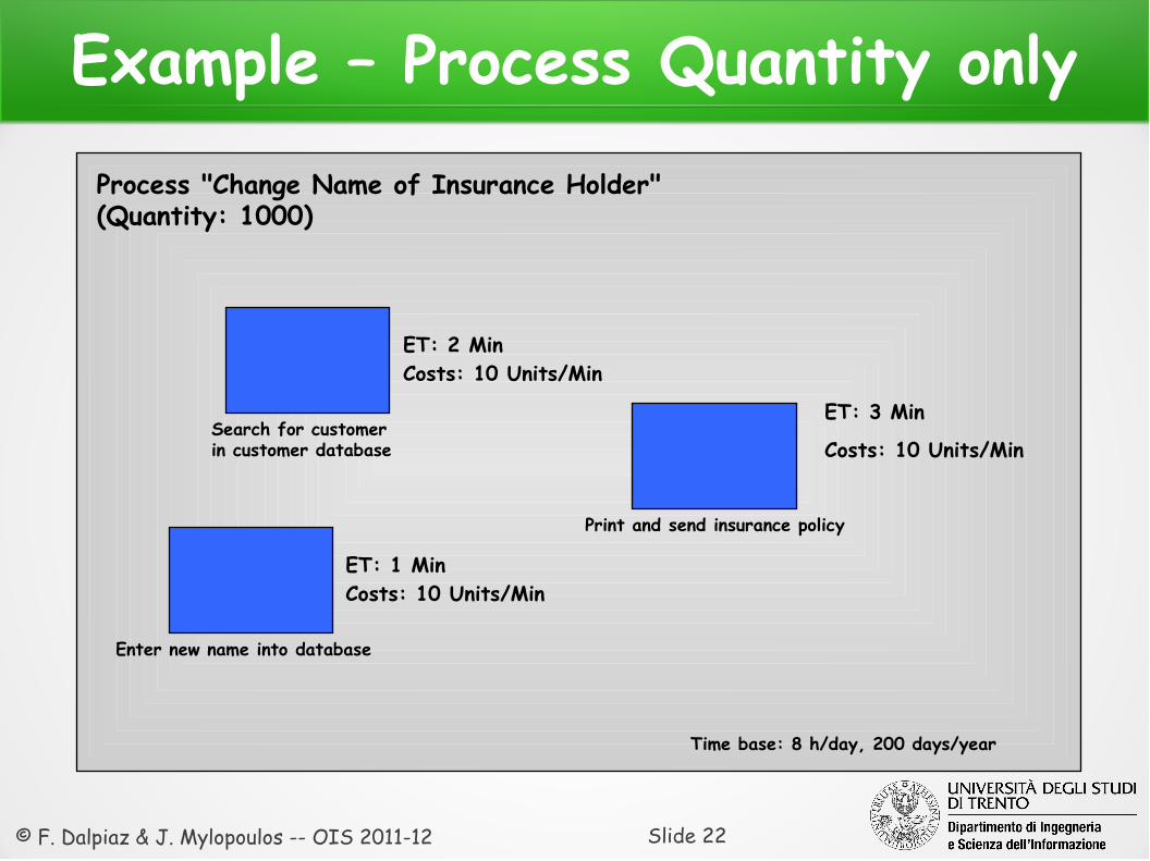
Example – Process Quantity onlyProcess "Change Name of Insurance Holder" (Quantity: 1000)

Search for customerin customer database

Enter new name into database

Print and send insurance policy

ET: 2 MinCosts: 10 Units/Min

ET: 1 MinCosts: 10 Units/Min

ET: 3 Min

Costs: 10 Units/Min

Time base: 8 h/day, 200 days/year


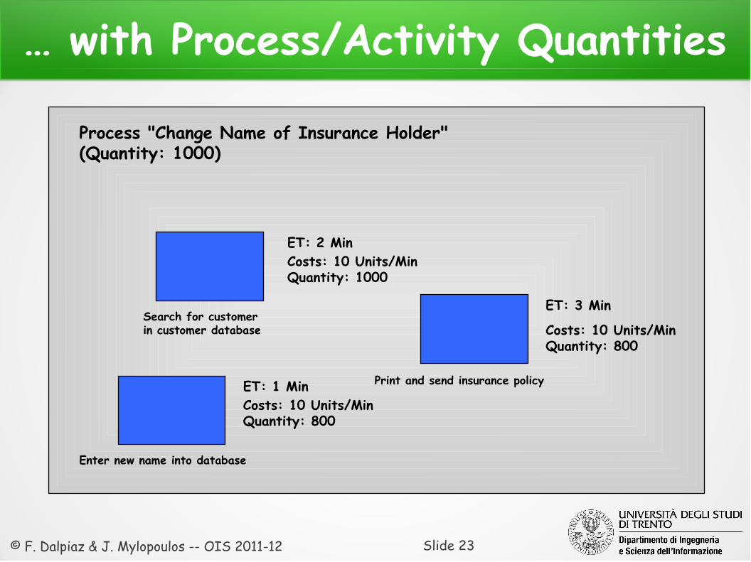
… with Process/Activity Quantities

Process "Change Name of Insurance Holder" (Quantity: 1000)

Search for customerin customer database

Enter new name into database

Print and send insurance policy

ET: 2 MinCosts: 10 Units/MinQuantity: 1000

ET: 1 MinCosts: 10 Units/MinQuantity: 800

ET: 3 Min

Costs: 10 Units/MinQuantity: 800


Example


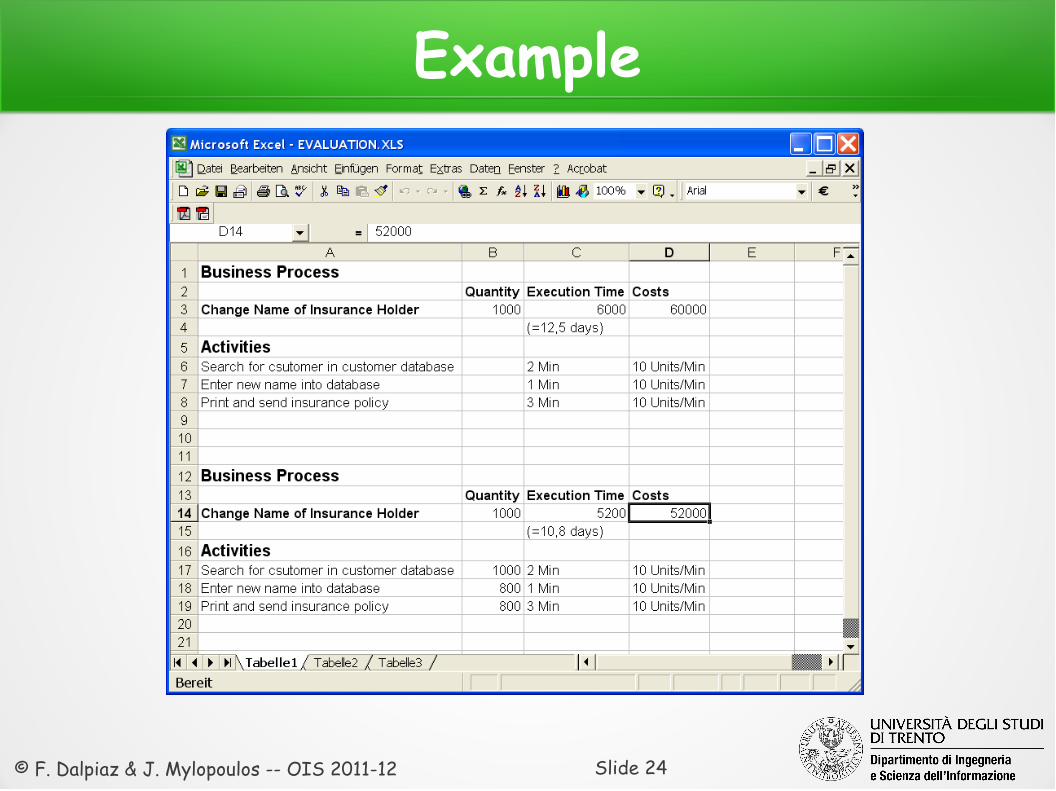
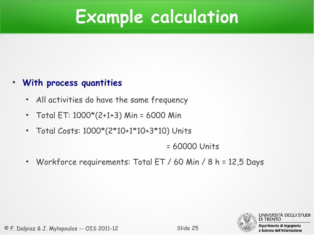
Example calculation

● With process quantities● All activities do have the same frequency● Total ET: 1000*(2+1+3) Min = 6000 Min● Total Costs: 1000*(2*10+1*10+3*10) Units

= 60000 Units● Workforce requirements: Total ET / 60 Min / 8 h = 12,5 Days


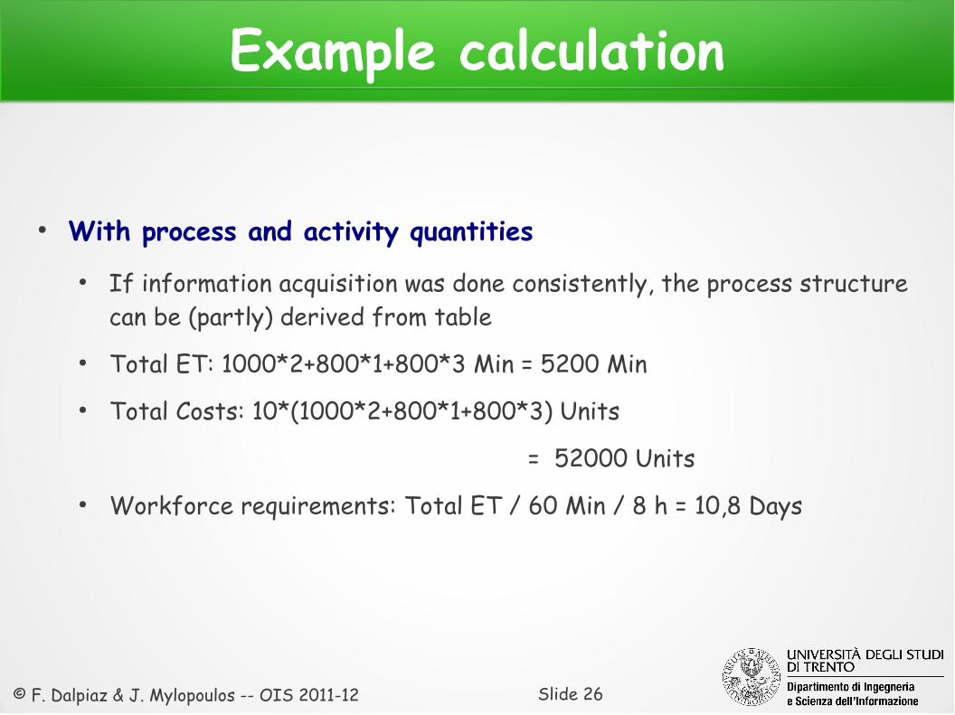
Example calculation

● With process and activity quantities● If information acquisition was done consistently, the process structure

can be (partly) derived from table● Total ET: 1000*2+800*1+800*3 Min = 5200 Min● Total Costs: 10*(1000*2+800*1+800*3) Units

= 52000 Units● Workforce requirements: Total ET / 60 Min / 8 h = 10,8 Days


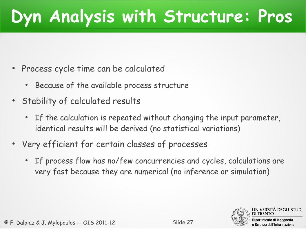
Dyn Analysis with Structure: Pros

● Process cycle time can be calculated● Because of the available process structure

● Stability of calculated results● If the calculation is repeated without changing the input parameter,

identical results will be derived (no statistical variations)

● Very efficient for certain classes of processes● If process flow has no/few concurrencies and cycles, calculations are

very fast because they are numerical (no inference or simulation)


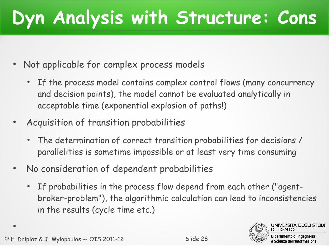
Dyn Analysis with Structure: Cons

● Not applicable for complex process models● If the process model contains complex control flows (many concurrency

and decision points), the model cannot be evaluated analytically in acceptable time (exponential explosion of paths!)

● Acquisition of transition probabilities● The determination of correct transition probabilities for decisions /

parallelities is sometime impossible or at least very time consuming

● No consideration of dependent probabilities● If probabilities in the process flow depend from each other ("agent-

broker-problem"), the algorithmic calculation can lead to inconsistencies in the results (cycle time etc.)

●


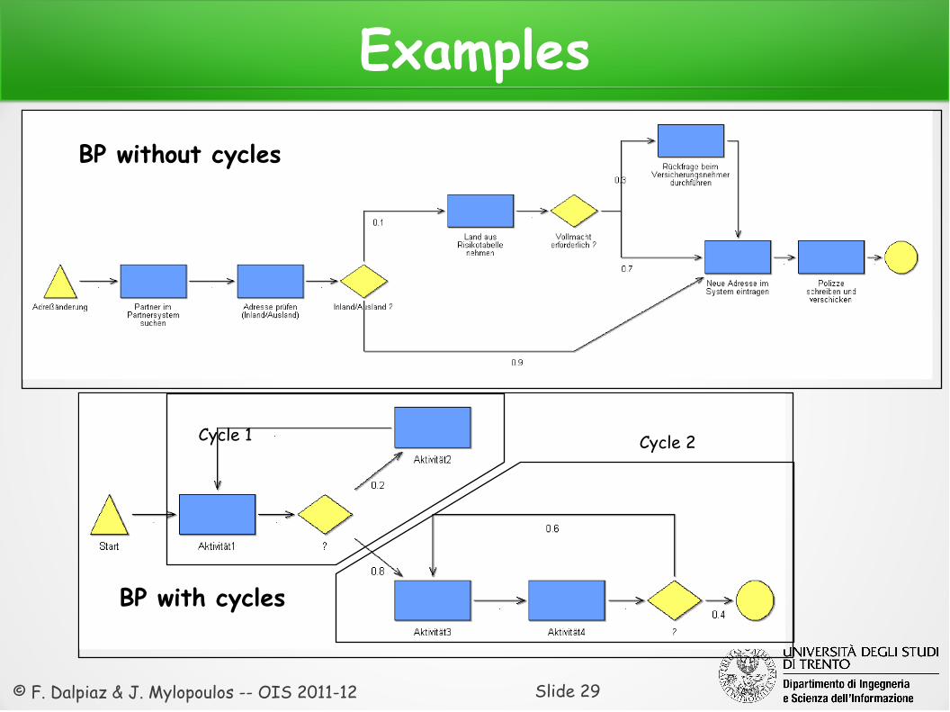
Examples

BP without cycles

BP with cycles

Cycle 1 Cycle 2


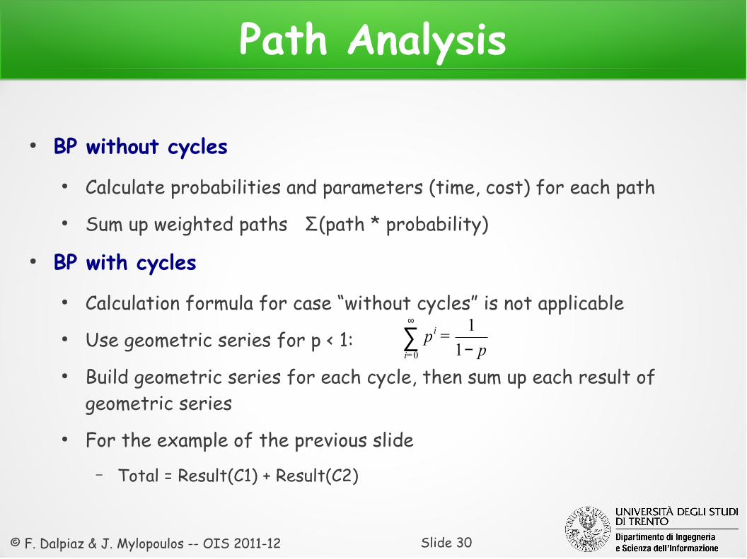
Path Analysis

● BP without cycles● Calculate probabilities and parameters (time, cost) for each path● Sum up weighted paths Σ(path * probability)

● BP with cycles● Calculation formula for case “without cycles” is not applicable● Use geometric series for p < 1: ● Build geometric series for each cycle, then sum up each result of

geometric series● For the example of the previous slide

– Total = Result(C1) + Result(C2)

p=p

=i

i

−∑∞

1

1

0


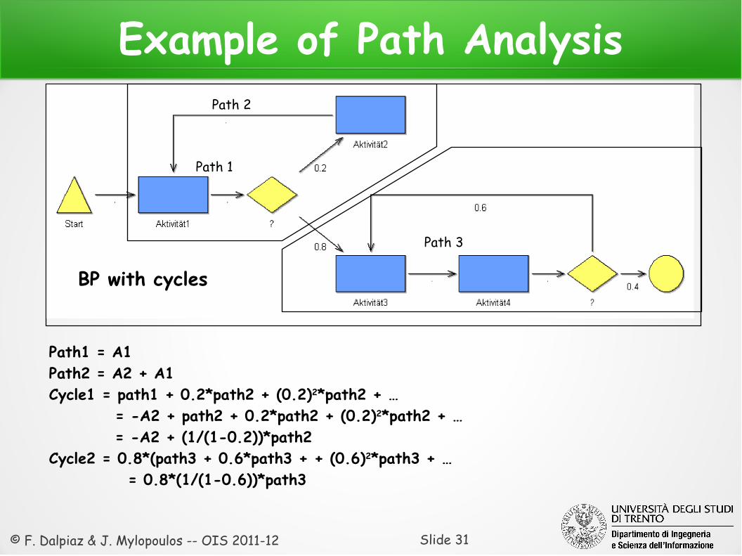
Example of Path Analysis

BP with cycles

Path 2

Path 3

Path1 = A1Path2 = A2 + A1Cycle1 = path1 + 0.2*path2 + (0.2)2*path2 + …

= -A2 + path2 + 0.2*path2 + (0.2)2*path2 + …= -A2 + (1/(1-0.2))*path2

Cycle2 = 0.8*(path3 + 0.6*path3 + + (0.6)2*path3 + … = 0.8*(1/(1-0.6))*path3

Path 1


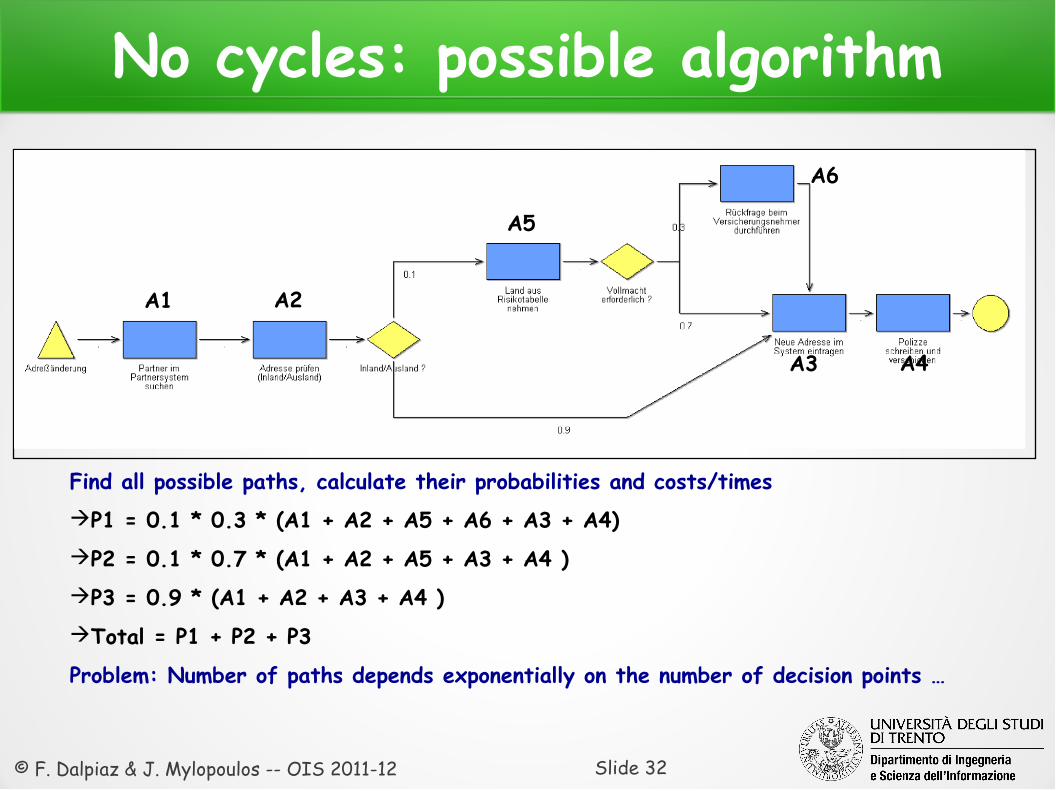
No cycles: possible algorithm

Find all possible paths, calculate their probabilities and costs/timesP1 = 0.1 * 0.3 * (A1 + A2 + A5 + A6 + A3 + A4) P2 = 0.1 * 0.7 * (A1 + A2 + A5 + A3 + A4 )P3 = 0.9 * (A1 + A2 + A3 + A4 )Total = P1 + P2 + P3

Problem: Number of paths depends exponentially on the number of decision points …

A1 A2

A3 A4

A5

A6


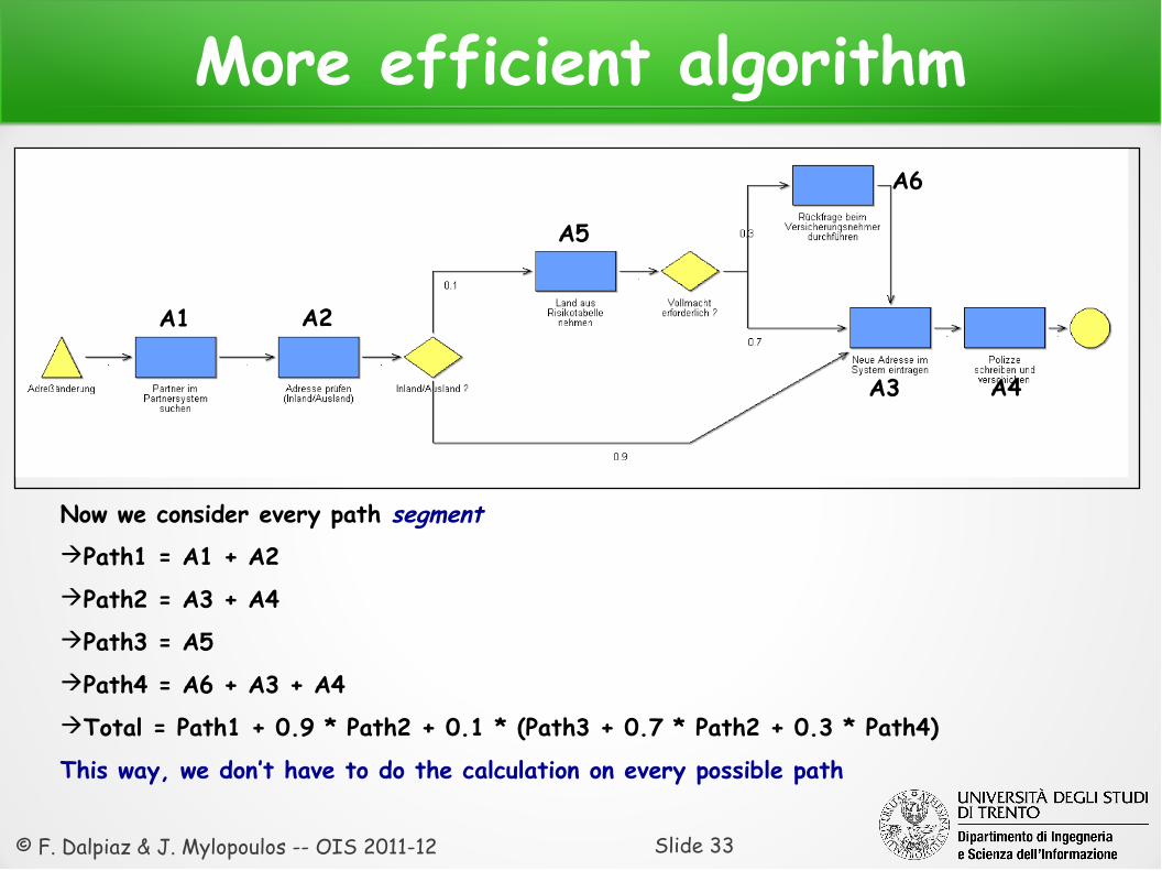
More efficient algorithm

Now we consider every path segmentPath1 = A1 + A2 Path2 = A3 + A4Path3 = A5Path4 = A6 + A3 + A4Total = Path1 + 0.9 * Path2 + 0.1 * (Path3 + 0.7 * Path2 + 0.3 * Path4)

This way, we don’t have to do the calculation on every possible path

A1 A2

A3 A4

A5

A6


… for cycles

Path1 = A1Path2 = A2 + A1Path3 = A3 + A4 Total = -A2 + 1/(1-0.2) * Path2 + 0.8 * 1/(1-0.6) * Path3 =

= -A2 + 1.25 * Path2 + 0.8 * 2.5 * Path3

A3 A4

Cycle 1Cycle 2

A1

A2


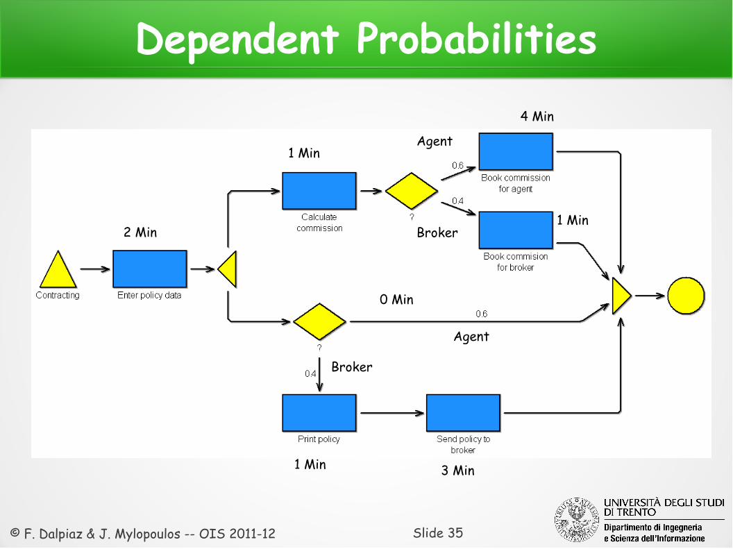
Dependent Probabilities

2 Min

0 Min

1 Min

1 Min 3 Min

4 Min

1 Min

Agent

Broker

Agent

Broker


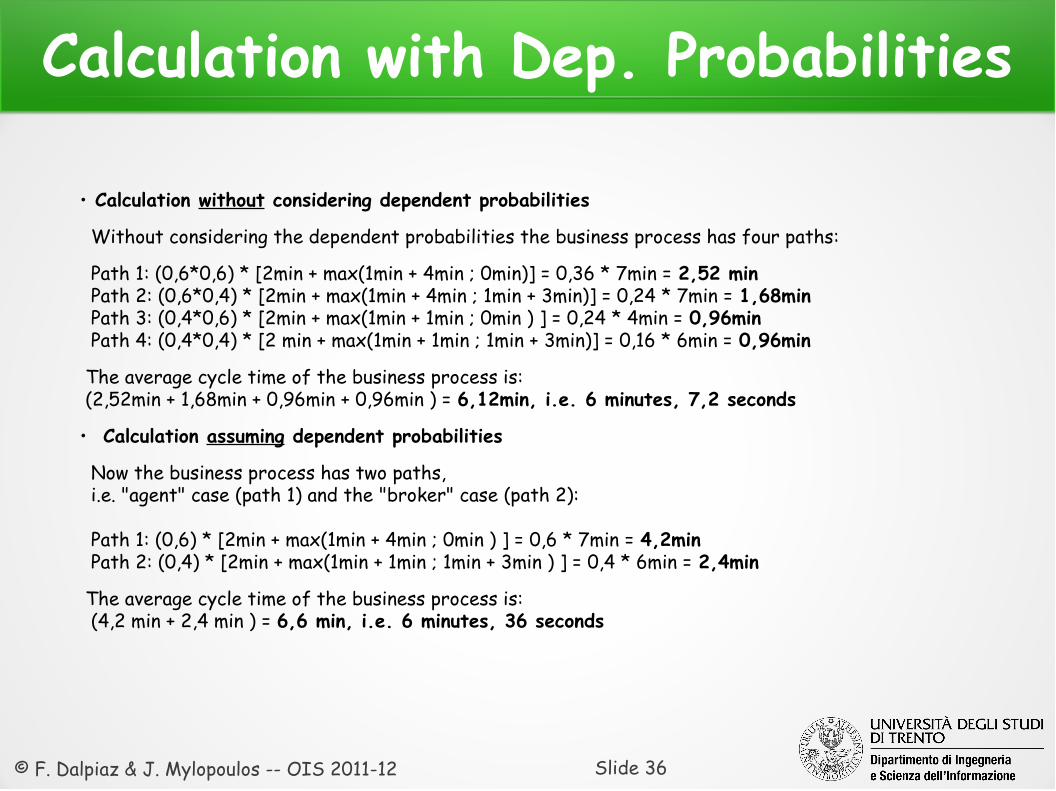
Calculation with Dep. Probabilities

• Calculation without considering dependent probabilities Without considering the dependent probabilities the business process has four paths: Path 1: (0,6*0,6) * [2min + max(1min + 4min ; 0min)] = 0,36 * 7min = 2,52 min Path 2: (0,6*0,4) * [2min + max(1min + 4min ; 1min + 3min)] = 0,24 * 7min = 1,68min Path 3: (0,4*0,6) * [2min + max(1min + 1min ; 0min ) ] = 0,24 * 4min = 0,96min Path 4: (0,4*0,4) * [2 min + max(1min + 1min ; 1min + 3min)] = 0,16 * 6min = 0,96min

The average cycle time of the business process is: (2,52min + 1,68min + 0,96min + 0,96min ) = 6,12min, i.e. 6 minutes, 7,2 seconds

• Calculation assuming dependent probabilities Now the business process has two paths, i.e. "agent" case (path 1) and the "broker" case (path 2):

Path 1: (0,6) * [2min + max(1min + 4min ; 0min ) ] = 0,6 * 7min = 4,2min Path 2: (0,4) * [2min + max(1min + 1min ; 1min + 3min ) ] = 0,4 * 6min = 2,4min

The average cycle time of the business process is: (4,2 min + 2,4 min ) = 6,6 min, i.e. 6 minutes, 36 seconds


Workforce Requirements

● Many (re-) organization projects target on cost and cycle time reduction. In many companies with intensive usage of human resources, a cost reduction can (only/mainly) be reached by reducing personnel costs

● For a business process, (abstract) workforce requirements can be calculated by considering the average execution time of a process and the number of times it is executed per year

● If the execution time per business process can be divided and assigned to groups of actors participating in the process, (concrete) workforce requirements can be calculated, e.g. at the levels of organizational units, roles etc.


BP Simulation: Idea

● Do not analyze analytically the process● No calculations needed here!

● Simulate a run-through on the model● E.g., whenever a decision point is found, take a decision!

● The more runs, the more accurate the results


BP Simulation: Pros

● All models – even complex ones – can be evaluated● The models to be evaluated can contain complex control flows

(concurrency and branches)

● Consideration of dependent probabilities● Dependent probabilities within a process are handled correctly ("agent-

broker-problem"). Additionally, the "business correctness" of the problem is ensured

● Cycle time can be calculated● Since process structure is available


BP Simulation: Cons

● Results can vary● Because of stochastic distributions influencing the variables and

transition conditions ( acceptance!)→

● Statistical knowledge, simulation basics may be missing● To apply simulation adequately, the user should have appropriate skills

and statistical knowledge


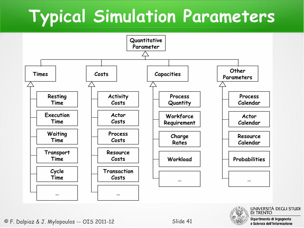
Typical Simulation Parameters

CostsTimes

QuantitativeParameter

Capacities OtherParameters

ExecutionTime

WaitingTime

RestingTime

TransportTime

CycleTime

…

ProcessQuantity

WorkforceRequirement

ChargeRates

Workload

…

ProcessCalendar

ActorCalendar

ResourceCalendar

Probabilities

…

ActorCosts

ProcessCosts

ActivityCosts

ResourceCosts

TransactionCosts

…


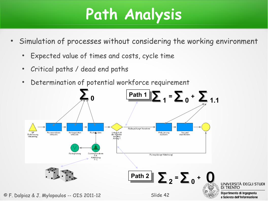
Path Analysis● Simulation of processes without considering the working environment

● Expected value of times and costs, cycle time● Critical paths / dead end paths● Determination of potential workforce requirement

ΣΣ 0 Path 1Path 1

Path 2Path 2

ΣΣ 0ΣΣ 1 ΣΣ 1.1= +

ΣΣ 0ΣΣ 2 00= +


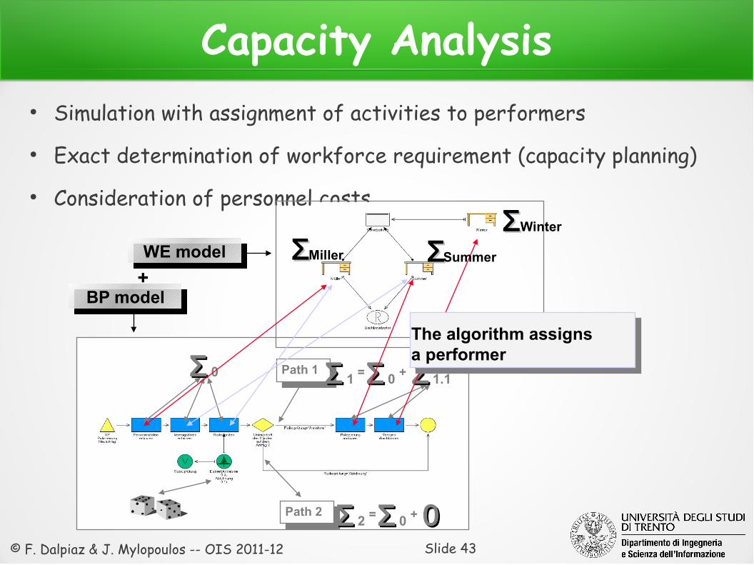
Capacity Analysis● Simulation with assignment of activities to performers● Exact determination of workforce requirement (capacity planning)● Consideration of personnel costs

ΣΣ 0 Path 1Path 1

Path 2Path 2

ΣΣ 0ΣΣ 1 ΣΣ 1.1= +

ΣΣ 0ΣΣ 2 00= +

The algorithm assignsa performer

ΣΣMiller ΣΣSummer

ΣΣWinter

BP modelBP model

WE modelWE model

+


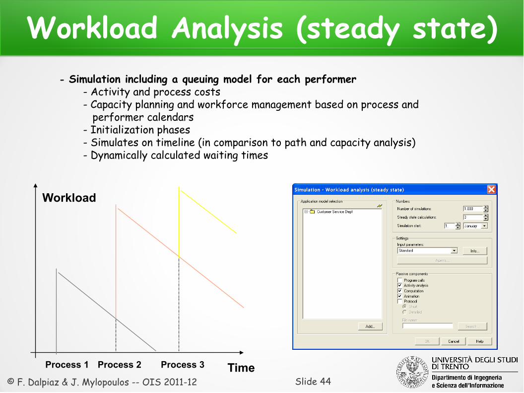
Workload Analysis (steady state)- Simulation including a queuing model for each performer

- Activity and process costs- Capacity planning and workforce management based on process and performer calendars- Initialization phases- Simulates on timeline (in comparison to path and capacity analysis)- Dynamically calculated waiting times

TimeProcess 1 Process 2 Process 3

Workload


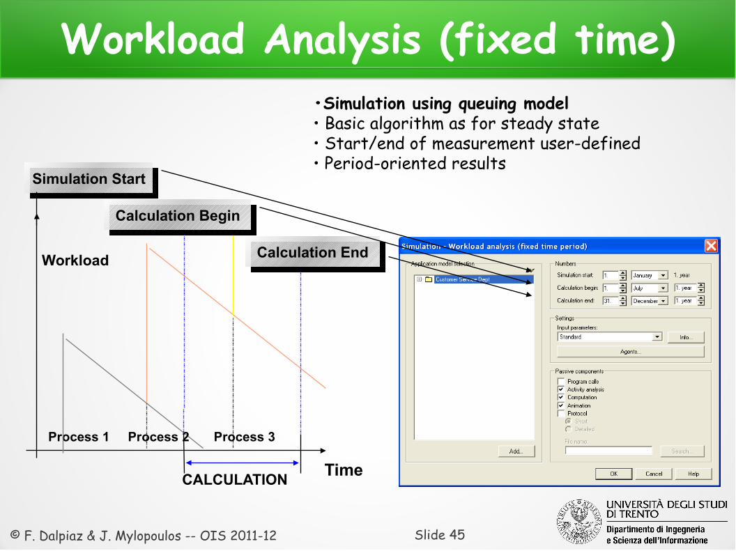
Workload Analysis (fixed time)

Simulation StartSimulation Start

•Simulation using queuing model• Basic algorithm as for steady state• Start/end of measurement user-defined• Period-oriented results

Time

Process 1 Process 2 Process 3

Workload

CALCULATION

Calculation BeginCalculation Begin

Calculation EndCalculation End


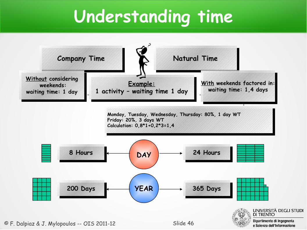
Understanding time

Company TimeCompany Time Natural TimeNatural Time

DAY

YEAR

8 Hours8 Hours

200 Days200 Days

24 Hours24 Hours

365 Days365 Days

Monday, Tuesday, Wednesday, Thursday: 80%, 1 day WTFriday: 20%, 3 days WTCalculation: 0,8*1+0,2*3=1,4

Monday, Tuesday, Wednesday, Thursday: 80%, 1 day WTFriday: 20%, 3 days WTCalculation: 0,8*1+0,2*3=1,4

Example:1 activity – waiting time 1 day

Example:1 activity – waiting time 1 day

Without considering weekends:

waiting time: 1 day

Without considering weekends:

waiting time: 1 dayWith weekends factored in:

waiting time: 1,4 daysWith weekends factored in:

waiting time: 1,4 days


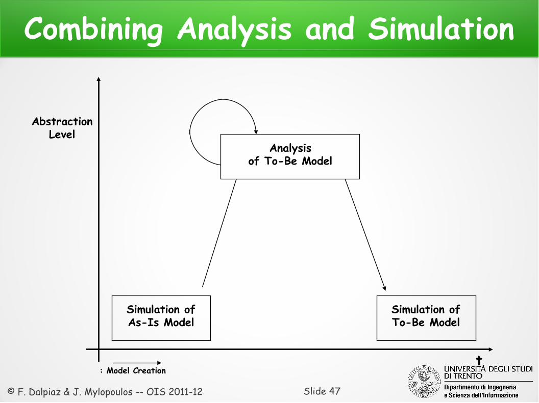
Combining Analysis and Simulation

t

AbstractionLevel

: Model Creation

Simulation ofAs-Is Model

Simulation ofTo-Be Model

Analysisof To-Be Model

Documents

15. Business Process Analysis and Simulationdisi.unitn.it/~dalpiaz/ois/lib/exe/fetch.php?media=15-bpanalysis.pdf · Business Process Analysis and Simulation ... Generating non-standard