Embed Size (px)
Citation preview

14.471: Public Economics
Capital Income Taxation
Emmanuel Saez
MIT: Fall 2009
1

MOTIVATION
1) Capital income is about 25% of national income (labor
income is 75%) but distribution of capital income is much
more unequal than labor income
Capital income inequality is due to differences in savings be-
havior but also inheritances received
⇒ Equity suggests it should be taxed more than labor
2) Capital Accumulation correlated strongly with growth [al-
though causality link is not obvious] and capital accumulation
might be sensitive to the net-of-tax return.
⇒ Efficiency cost of capital taxation might be high.
2

MOTIVATION
3) Capital more mobile internationally than labor ⇒ Incidence
of capital taxation might fall on workers:
Open economy with fully mobile capital, net-of-tax rate of
return is fixed by the international rate of return r∗ so that
(1− �)f ′(k) = r∗ where k is capital stock per person
Wage w = f(k)− r∗k falls with �
4) Capital taxation is extremely complex and provides many
tax avoidance opportunities.
3
MACRO FRAMEWORK
Constant return to scale aggregate production:
Y = F (K,L) = rK + wL = output = income
K = capital stock (wealth), L = labor input
r = rate of return on capital, w is wage rate
rK = capital income, wL = labor income
� = rK/Y = capital income share (constant � when F (K,L) =K�L1−� Cobb-Douglas), � ≃ 30%
� = K/Y = wealth to annual income ratio, � ≃ 5− 6
r = (rK/Y ) ⋅ (Y/K) = �/�, r = 5− 6%
Infinite horizon model: U =∑t u(ct)/(1+�)t ⇒ r = � (discount
rate) and � = �/�
4

SAVING FLOWS
Saving is a flow and wealth or net worth is a stock
Three saving flows:
1) Personal saving: individual income less individual con-sumption [fell dramatically in the US since 1980s, recent ↑since 2008]
2) Corporate Saving: retained earnings = after tax profits -distributions to shareholders
3) Government Saving: Taxes - Expenditures [federal, stateand local]
Taxes on savings might affect different savings flows differ-ently: savings subsidy through a tax credit can ↑ individualsavings but ↓ govt saving [if govt spending stays constant]
5

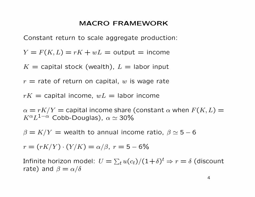
FACTS ABOUT WEALTH AND CAPITAL INCOME
Definition: Capital Income = Returns from Wealth Holdings
Aggregate US Personal Wealth = 3.5*GDP = $ 50 Tr
Tangible assets: residential real estate (land+buildings) [in-come = rents] and unincorporated business + farm assets[income = profits]
Financial assets: corporate stock [income = dividends + re-tained earnings], fixed claim assets (corporate and govt bonds,bank accounts) [income = interest]
Liabilities: Mortgage debt, Consumer credit debt
Substantial amount of financial wealth is held indirectly through:pension funds [DB+DC], mutual funds, insurance reserves
6

CAPITAL INCOME IN NATIONAL ACCOUNTS
Gross capital income (before depreciation) is about 40% of
GDP
Net capital income (after depreciation) is about 25% of per-
sonal income
The capital income share in total income is relatively stable in
the long-run (but with some short term fluctuations)
Average real rate of return of capital around 5-6%, varies
greatly from year to year
7
FACTS ABOUT WEALTH AND CAPITAL INCOME
Wealth = W , Return = r, Capital Income = rW
Wt = Wt−1 + rtWt−1 + Et + It − Ct
where Wt is wealth at age t, Ct is consumption, Et labor in-
come earnings (net of taxes), rt is the average (net) rate of
return on investments and It net inheritances (gifts received
and bequests - gifts given).
Replacing Wt−1 and so on, we obtain the following expression
(assuming initial wealth W0 is zero):
Wt =t∑
k=1
(Ek − Ck + Ik)t∏
j=k+1
(1 + rj)
8

FACTS ABOUT WEALTH AND CAPITAL INCOME
Wt =t∑
k=1
(Ek − Ck + Ik)t∏
j=k+1
(1 + rj)
Differences in Wealth and Capital income due to:
1) Age, past earnings, and past saving behavior Et − Ct [life
cycle wealth]
2) Net Inheritances received It [transfer wealth]
3) Rates of return rt
[more details in Davies-Shorrocks ’00, Handbook of Income
Distribution]
9

WEALTH DISTRIBUTION
Wealth inequality is very large
US Household Wealth is divided 1/3,1/3,1/3 for the top 1%,
the next 9%, and the bottom 90% [bottom 1/3 households
hold almost no wealth]
Financial wealth is more unequally distributed than (net) real
estate wealth
Share of real estate wealth falls at the top of the wealth dis-
tribution
Growth of private pensions [such as 401(k) plans] has “de-
mocratized” stock ownership in the US
10
WEALTH DISTRIBUTION
Wealth is more unequally distributed than income [true in allcountries]
Top 1% income share in the US is around 20%
Top 1% labor income share in the US (among workers) isaround 15%
US Income concentration has ↑ sharply since 1970:
top 1% income share was 9% in 1970 and 23.5% in 2007[Piketty-Saez QJE’03 updated]
US Wealth concentration has only slightly increased:
Top 1% wealth share has grown “only” from 31% in 1962to 34% in 2007 based on the Survey of Consumer Finances[Scholz ’03, Kennickell ’09]
11
FACTS OF US CAPITAL INCOME TAXATION
Good US references: Gravelle ’94 book, Slemrod-Bakija ’04
book
1) Corporate Income Tax (fed+state): 35% Federal tax rate
on profits of corporations [complex rules with many industry
specific provisions]
2) Individual Income Tax (fed+state): taxes many forms of
capital income
Realized capital gains and dividends (dividends since ’03 only)
receive preferential treatment
Imputed rent of home owners, returns on pension funds, state+local
bonds interest are exempt
12
FACTS OF US CAPITAL INCOME TAXATION
3) Estate and gift taxes:
Fed taxes estates above $3.5M exemption (only .2% of de-ceased liable), top rate is 45%
Charitable and spousal giving is exempt
Substantial tax avoidance activity through tax accountants
Step-up of realized capital gains at death (lock-in effect)
4) Property taxes (local) on real estate (old tax):
Tax varies across jurisdictions. About 0.5% of market valueon average, like a 10% tax on imputed rent if return is 5%
Lock-in effect in states that use purchase price base such asCalifornia
13

LIFE CYCLE MODEL OF WEALTH (MODIGLIANI)
Individuals work for R years and live for T years: T − R is
retirement duration
Individuals earn income wt from period 0 to R and earn zero
afterwards
Individuals have additive separable utility∑Tt=1 u(ct)/(1 + �)t
with concave u(.)
subject to inter-temporal budget constraint:∑Tt=1 ct/(1+r)t ≤∑R
t=1wt/(1 + r)t (multiplier �)
FOC: u′(ct)/(1 + �)t = �/(1 + r)t
Euler equation: u′(ct+1)/u′(ct) = (1 + �)/(1 + r)
14
LIFE CYCLE MODEL OF WEALTH (MODIGLIANI)
Euler equation: u′(ct+1)/u′(ct) = (1 + �)/(1 + r)
If � < r, ct+1 > ct ⇒ Individuals save to consume more lateron
If � > r, ct+1 < ct ⇒ Individuals want to consume more earlieron
If � = r then ct is constant with t:
⇒ Individuals want to smooth consumption by saving whileworking and consuming saving while retired ⇒ Wealth Wt isinversely U-shaped during life-cycle
⇒ Wealth inequality only slightly higher than labor incomeinequality [does not fit facts]
15

OTHER FACTORS AFFECTING WEALTH
DISPERSION
1) Heterogeneity in tastes for saving:
∙ traditional discount rate
∙ self-control problems [hyperbolic discount rate] and financial
education
2) Rates of returns received on assets: traditional risk aver-
sion, luck, but also financial education
3) Net inheritances and gifts received [in general from parents]
16
LIFE CYCLE VS. INHERITED WEALTH
Old view: Tobin and Modigliani: life cycle wealth accounts
for the bulk of the wealth hold in the US. Kotlikoff-Summers
JPE’81 challenged the old view.
Debate: Kotlikoff vs. Modigliani in JEP’88.
Why is this question important?
1) Economic Modelling: what accounts for wealth accumula-
tion and inequality? Is widely used life-cycle model with no
bequests a good approximation? [Causality between growth
and savings]
2) Policy Implications: taxation of capital income and estates.
Role of pay-as-you-go vs. funded retirement programs
17
LIFE CYCLE VS. INHERITED WEALTH
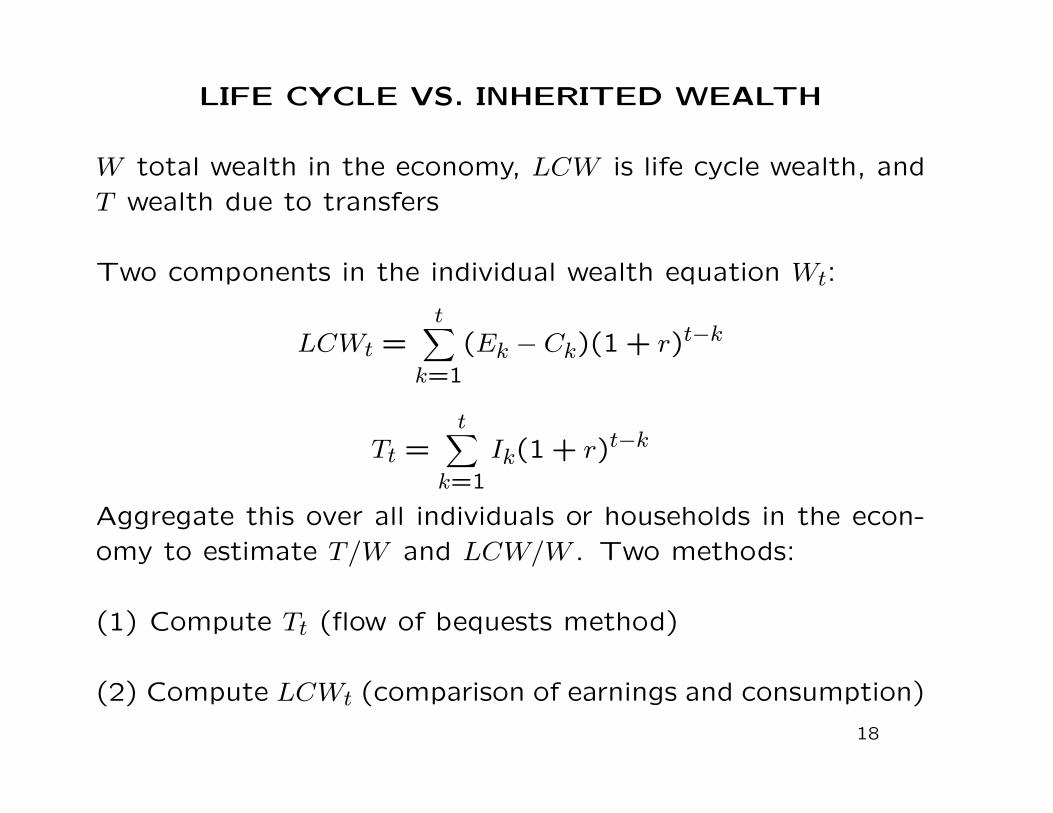
W total wealth in the economy, LCW is life cycle wealth, andT wealth due to transfers
Two components in the individual wealth equation Wt:
LCWt =t∑
k=1
(Ek − Ck)(1 + r)t−k
Tt =t∑
k=1
Ik(1 + r)t−k
Aggregate this over all individuals or households in the econ-omy to estimate T/W and LCW/W . Two methods:
(1) Compute Tt (flow of bequests method)
(2) Compute LCWt (comparison of earnings and consumption)
18
44 Economic Perspectives
In Hundreds 70 Of Dollars
60
50 ..
40.
30 ;-*** * s EARNINGS
20 -CONSUMPTION
10 10
20 30 40 50 60 70 Age 1910 1920 1930 1940 1950 1960 Year
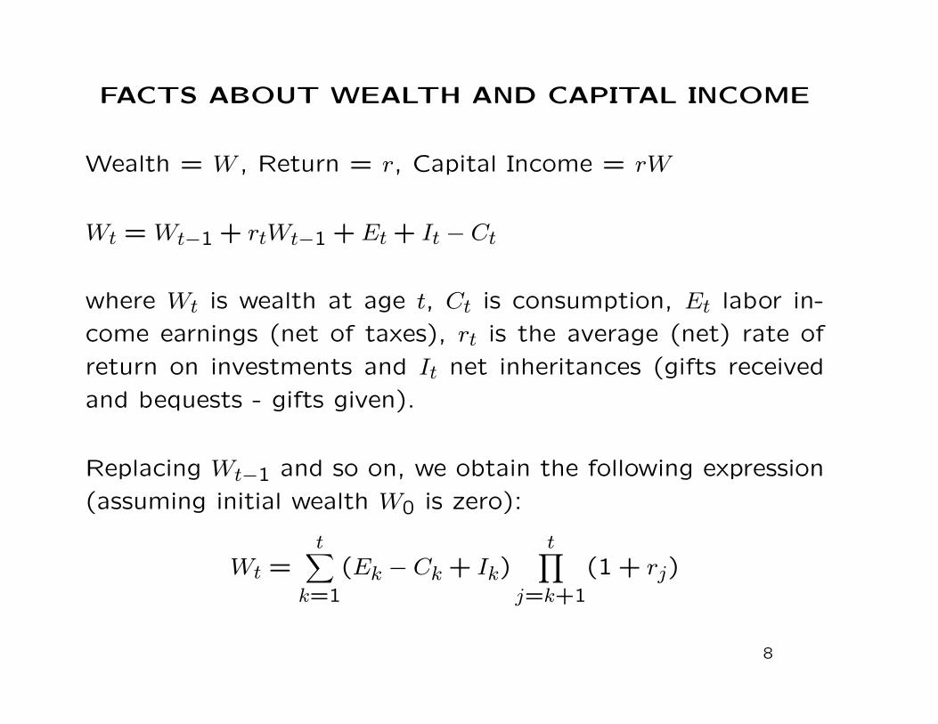
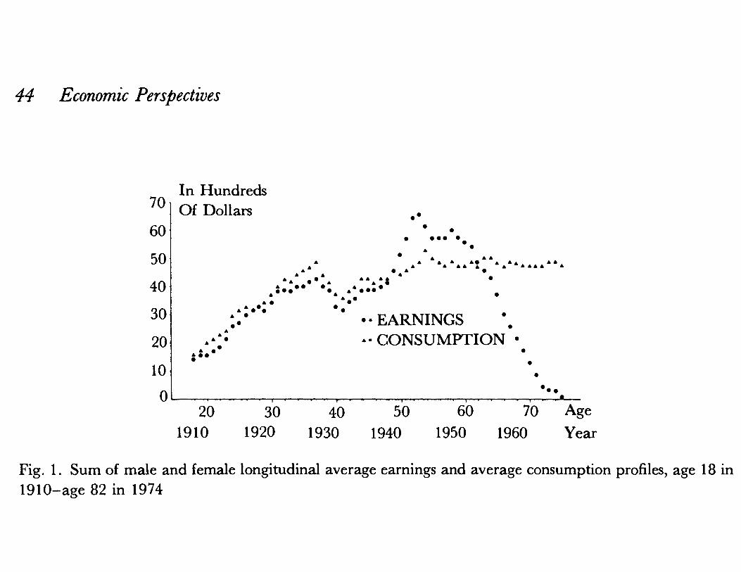
Fig. 1. Sum of male and female longitudinal average earnings and average consumption profiles, age 18 in 1910-age 82 in 1974
percent of U.S. private net worth is devoted to future consumption, with the rest destined for intergenerational transfer. White (1978) used aggregate data on the age structure of the population, age earnings and age consumption profiles along with a variety of parametric assumptions and concludes that the life cycle model can account for only about a quarter of aggregate saving. Though their accounting frameworks are somewhat different and though they use different data, and only cross section data at that, Darby and White reach essentially the same conclusion as Kotlikoff and Summers because the basic shapes of U.S. cross section age earnings and age consumption profiles and the longitudinal profiles that can reasonably be inferred from the cross section profiles are quite different from those of the textbook life cycle model.
Calculations of Life Cycle and Transfer Wealth Using Flow Data The analyses just described directly calculate life cycle wealth and indirectly infer
the stock of transfer wealth. Obviously it would be very useful to corroborate these results with direct evidence on intergenerational transfers. Kotlikoff and Summers
128 In Hundreds Of Dollars
112.
96-
80s
64 .- .. EARNINGS
48 .- * * CONSUMPTION
32 .
1 6 1 0 . . . . . . . - . . . , . 20 30 40 50 60 70 Age
1940 1950 1960 1970 Year
Fig. 2. Sum of male and female longitudinal average earnings and average consumption profiles, age 18 in 1940-age 52 in 1974. Reproduced by permission of the University of Chicago Press.
LIFE CYCLE VS. INHERITED WEALTH
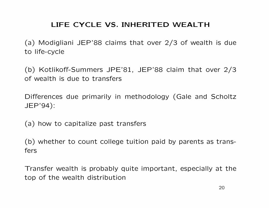
(a) Modigliani JEP’88 claims that over 2/3 of wealth is dueto life-cycle
(b) Kotlikoff-Summers JPE’81, JEP’88 claim that over 2/3of wealth is due to transfers
Differences due primarily in methodology (Gale and ScholtzJEP’94):
(a) how to capitalize past transfers
(b) whether to count college tuition paid by parents as trans-fers
Transfer wealth is probably quite important, especially at thetop of the wealth distribution
20

152 Journal of Economic Perspectives
Table 4 Intergenerational Transfers as a Source of Capital Accumulation, 1986
Stock of Transfer Wealth Annual Flow ($ billions)
Transfer Category ($ billions) (r - n = 0.01)
Support Given to: Children 32.69 1346.7 Parents 3.37 -104.3 Grandparents 0.07 -4.0 Grandchildren 5.05 416.2
Trusts 14.17 576.1 Life Insurance 7.84 258.3
Totals Intended Transfers 63.19 2489.3 College Payments 35.29 1441.5 Bequests 105.00 3708.1
As a % of net wortha Intended Transfers 0.53 20.8 College Expenses 0.29 12.0 Bequests 0.88 31.0
Source: Authors' calculations from the Survey of Consumer Finances. aAggregate net worth in the SCF in 1986 is $11,976 billion.
transfers and then convert the flow to a stock using steady-state assumptions. This produces a lower-bound estimate of wealth due to intended transfers.7 Details of these calculations can be found in the first part of the Appendix.
The first column of Table 4 presents our estimates that the gross flow of intended transfers in 1986 was about $63 billion, with the majority being support given from one household to another. The annual total of college payments was another $35 billion, and estimated bequests were another $105 billion. Our next task was to convert the annual flow of transfers into a stock of wealth. The equations behind this calculation appear in the second part of the Appendix. The conversion of a flow of transfers into a stock of transfer wealth requires obtaining values for a number of parameters: the flow of transfers in the current year (denoted by t), the growth rate of transfers (n), the interest rate (r), and the ages at which people receive transfers (I), give transfers (G), and die (D).
These parameters can be inferred from a variety of sources. For example, Kotlikoff and Summers (1981) estimate historical averages of a real rate of return of r = .045 and a real rate of GDP growth of .035. We set the growth
7Life-cycle wealth cannot be inferred by taking the difference between estimated intended transfer wealth and net worth, because some of that difference is due to intended bequests.
LIFE CYCLE VS. INHERITED WEALTH
More interesting question: how do the shares of inheritancevs. life-cycle evolve over time?
Inheritance share likely huge in the distant past: class societywith rentiers vs. workers [Delong ’03]
Inheritance share likely ↓ in 20th century but might have ↑recently (Piketty ’10 for France)
Post-war period was a time of fast population growth and fasteconomic growth ⇒ If n (growth) large relative to r (rate ofreturn on wealth) ⇒ Inheritances play a minor role in life-timewealth
Could be an exceptional episode and Western countries aregoing back to earlier situation where inheritances were impor-tant
22

KEY ELEMENTS OF DEBATE ON CAPITAL
INCOME TAXATION
Economic debate:
1) Distributional concerns: capital income accrues dispropor-tionately to higher income families
2) Efficiency concerns: capital tax distorts savings, businesscreation, capital mobility across countries
Public policy debate:
3) Should we tax income vs. consumption? [Fundamental taxreform debate]
4) Should we encourage savings by cutting tax on capital in-come or with tax favored savings vehicles?
23

TAXES IN OLG LIFE-CYCLE MODEL
max U = u(c1, l1) + �u(c2, l2)
No tax situation: earn w1l1 in period 1, w2l2 in period 2
Savings s = w1l1 − c1, c2 = w2l2 + (1 + r)s
Capital income rs
Intertemporal budget with no taxes:
c1 + c2/(1 + r) ≤ w1l1 + w2l2/(1 + r)
This model has uniform rate of return and does not capture
excess returns
24
TAXES IN OLG MODEL
Budget with consumption tax tc:
(1 + tc)[c1 + c2/(1 + r)] ≤ w1l1 + w2l2/(1 + r)
Budget with labor income tax �L:
c1 + c2/(1 + r) ≤ (1− �L)[w1l1 + w2l2/(1 + r)]
Consumption and labor income tax are equivalent if
1 + tc = 1/(1− �L)
Both taxes distort only labor-leisure choice
25

TAXES IN OLG MODEL
Budget with capital income tax �K:
c1 + c2/(1 + r(1− �K)) ≤ w1l1 + w2l1/(1 + r(1− �K))
�K distorts only inter-temporal consumption choice
Budget with comprehensive income tax � :
c1 + c2/(1 + r(1− �)) ≤ (1− �)[w1l1 + w2l2/(1 + r(1− �))]
� distorts both labor-leisure and inter-temporal consumption
choices
� imposes “double” tax: (1) tax on earnings, (2) tax on sav-
ings
26
EFFECT OF r ON SAVINGS
Assume that labor supply is fixed. Suppose r ↑:
1) Substitution effect: price of c2 ↓ ⇒ c2 ↑, c1 ↓ ⇒ savings
s = w1l1 − c1 ↑.
2) Wealth effect: Price of c2 ↓ ⇒ both c1 and c2 ↑ ⇒ save less
3) Human wealth effect: present discounted value of labor
income ↓ ⇒ both c1 and c2 ↓ ⇒ save more
Note: If w2l2 < c2 (ie s > 0), 2)+3) ⇒ save less
Total net effect is theoretically ambiguous ⇒ �K has ambigu-
ous effects on s
27

SHIFT FROM LABOR TO CONSUMPTION TAX
Labor and consumption are equivalent for the individual if 1 +tc = 1/(1− �L) but savings pattern is different
Assume w2 = 0 and l1 = 1
(1 + tc)[c1 + c2/(1 + r)] = w1 with consumption tax
c1 + c2/(1 + r) = (1− tL)w1 with labor tax
1) Consumption tax tc: cc1 = (w1 − sc)/(1 + tc), cc2 = (1 +r)sc/(1 + tc)
2) Labor income tax �L: cL1 = w1(1− �L)− sL, cL2 = (1 + r)sL
Same consumption in both cases so sL = sc/(1 + tc) ⇒ Savemore with a consumption tax
28
TRANSITION FROM LABOR TO C TAX
In OLG model and closed economy, capital stock is due to
life-cycle savings s
Start a labor tax �L and you decide to switch to a consumption
tax tc
The old [at time of transition] would have paid nothing in
labor tax regime but now have to pay tax on c2
For the young [and future generations], the two regimes look
equivalent so they now save more and increase the capital
stock
However, this increase in capital stock comes at the price of
hurting the old who are taxed twice
29
TRANSITION FROM LABOR TO C TAX
Suppose the government keeps the old as well off as in previoussystem by exempting them from consumption tax
This creates a deficit in government budget equal to
d = �Lw1 − tcc1 = tcw1/(1 + tc)− tcc1 = tcsL
Extra saving by the young is sc − sL = tcsL exactly equal togovernment deficit.
Full neutrality result: Extra savings of young is equal to oldcapital stock + new government deficit ⇒ no change in theaggregate capital stock
Full neutrality depends crucially on same r for govt debt andaggregate r [in practice: equity premium puzzle]
[Same result for Social Security privatization]
30
AUERBACH-KOTLIKOFF ’87 MODEL
Develop an inter-temporal Computational General Equilibrium(CGE) model:
1) Life cycle model, no bequests, people live for 55 years (bornat age 21). Work for 45 years, and retire for 10 years.
2) Only one individual per cohort, representative agent model [Useful for redistribution analysis across cohorts but not withincohorts]
3) Stock of wealth = life cycle savings [Classical Modiglianigraph]
4) Labor income tax distorts labor supply, capital income taxdistorts savings choice.
CES utility, discount rate, path of earnings with life cycle.
31

AUERBACH-KOTLIKOFF ’87: RESULTS
Tax reform experiments: shift from comprehensive income tax
to either
(a) pure consumption tax
(b) pure wage income tax
(c) pure capital income tax
[budget neutral but no transitional compensation]
32

Intertemporal
Elasticity of
Substitution
(γ)
Elasticity of
Substitution
between
consumption
and leisure
(ρ)
Elasticity
of
Substitution
in
Production
(σ)
Steady State
Efficiency
Gain from
Consumption
Tax (%
Lifetime
Wealth)
Steady State Change in Real
Wage (%)
Consumption
Tax
Wage
Tax
Capital
Income
Tax
0.25 0.80 1.0 0.29% 6% 2% -13%
0.10 0.80 1.0 0.37 6 2 -8
0.50 0.80 1.0 0.28 6 3 -17
0.25 0.30 1.0 0.25 6 2 -12
0.25 1.50 1.0 0.36 5 2 -13
0.25 0.80 0.8 0.19 4 2 -16
0.25 0.80 1.25 0.45 8 2 -9
All policy experiments are relative to an income tax at an initial tax rate of 15%.
Source: Auerbach and Kotlikoff (1987, Table 5.4).

AUERBACH-KOTLIKOFF ’87: RESULTS
1) Effect on capital stock:
(a) Consumption tax is best (because no compensation of the
old)
(b) Wage income tax has limited impact on capital stock
(c) Capital income tax is worst (significant elasticity of savings
wrt to r).
34

AUERBACH-KOTLIKOFF ’87: RESULTS
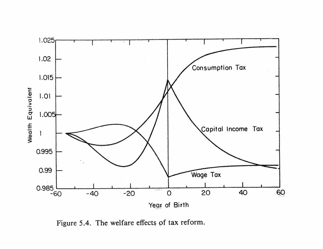
2) Effect on welfare measured in percentage increase of con-
sumption for each generation:
Consumption tax hurts current old and benefits the young and
future generations [no transitional relief]
Wage income tax benefits the old but hurts the young
Capital income tax hurts current generation (double tax), ben-
efits next generation (implicit levy of previously accumulated
capital) but hurts future generations (inefficient)
Key lessons: Transitional reliefs rules and anticipated vs. not
tax changes has large impact on results
35
OPTIMAL CAPITAL INCOME TAXATION
Complex problem with many sub-literatures: Banks and Dia-
mond Mirrlees Review ’09 provide excellent recent survey
1) Life-cycle models [linear and non-linear earnings tax]
2) Models with bequests [many models including the infinite
horizon model]
3) Models with future earnings uncertainty: New Dynamic
Public Finance [Kocherlakota ’09 book]
Bigger gap between theory and policy practice than in the case
of static labor income taxation
36
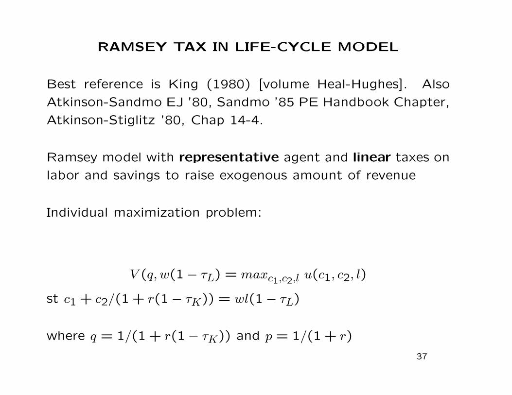
RAMSEY TAX IN LIFE-CYCLE MODEL
Best reference is King (1980) [volume Heal-Hughes]. Also
Atkinson-Sandmo EJ ’80, Sandmo ’85 PE Handbook Chapter,
Atkinson-Stiglitz ’80, Chap 14-4.
Ramsey model with representative agent and linear taxes on
labor and savings to raise exogenous amount of revenue
Individual maximization problem:
V (q, w(1− �L) = maxc1,c2,l u(c1, c2, l)
st c1 + c2/(1 + r(1− �K)) = wl(1− �L)
where q = 1/(1 + r(1− �K)) and p = 1/(1 + r)
37

RAMSEY CAPITAL INCOME TAX
Optimal tax rates can be obtained by solving the standard
Ramsey problem:
max V (q, w(1− �L))
st wl�L + (q − p)c2 ≥ g (�)
where g is exogenous tax revenue requirement
Can apply the results from the 3 good Ramsey model
Derive FOC for �K and �L
Can express them in terms of compensated elasticities
38

RAMSEY CAPITAL INCOME TAX
Combining the two FOC to get rid of �, you get:
r�K1 + r
(�L2 − �22) =�L
1− �L(�LL − �2L)
where �LL = (w(1− �L)/l)∂lc/∂(w(1− �L)) > 0 is the compen-
sated elasticity of labor supply with to wage rate.
�22 = (q/c2)∂cc2/∂q < 0
�L2 = (q/l)∂lc/∂q
�2L = (w(1− �L)/c2)∂cc2/∂(w(1− �L))
Formula defines relative optimal rates of taxation on labor and
capital (absolute levels depend on g)
39
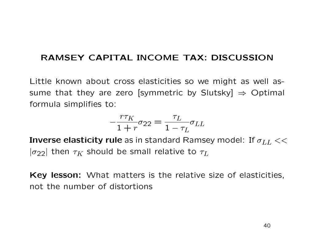
RAMSEY CAPITAL INCOME TAX: DISCUSSION
Little known about cross elasticities so we might as well as-
sume that they are zero [symmetric by Slutsky] ⇒ Optimal
formula simplifies to:
−r�K
1 + r�22 =
�L1− �L
�LL
Inverse elasticity rule as in standard Ramsey model: If �LL <<
∣�22∣ then �K should be small relative to �L
Key lesson: What matters is the relative size of elasticities,
not the number of distortions
40

FELDSTEIN JPE’78
Feldstein JPE’78 makes famous theoretical argument why �22can be large even if "usq = (q/s)∂s/∂q [uncompensated savingselasticity] is zero: Budget c1 + qc2 = w(1− �L)l + y
Slutsky equation [y is endowment =0 in equilibrium]: ∂cc2/∂q =∂c2/∂q + c2∂c2/∂y ⇒
�22 = "u2q + q∂c2/∂y
c2 = s/q so "u2q = (q/c2)∂c2/∂q = "usq − 1 ⇒
�22 = "usq − 1 + q∂c2/∂y
c1+qc2 = w(1−�L)l+y ⇒ ∂c1/∂y+q∂c2/∂y = w(1−�L)∂l/∂y+1 ≃ 1 (small income effects on labor supply)
�22 ≃ "usq + ∂c1/∂y ≃ ∂c1/∂y ≥ 0.75 [as saving rate modest]
41
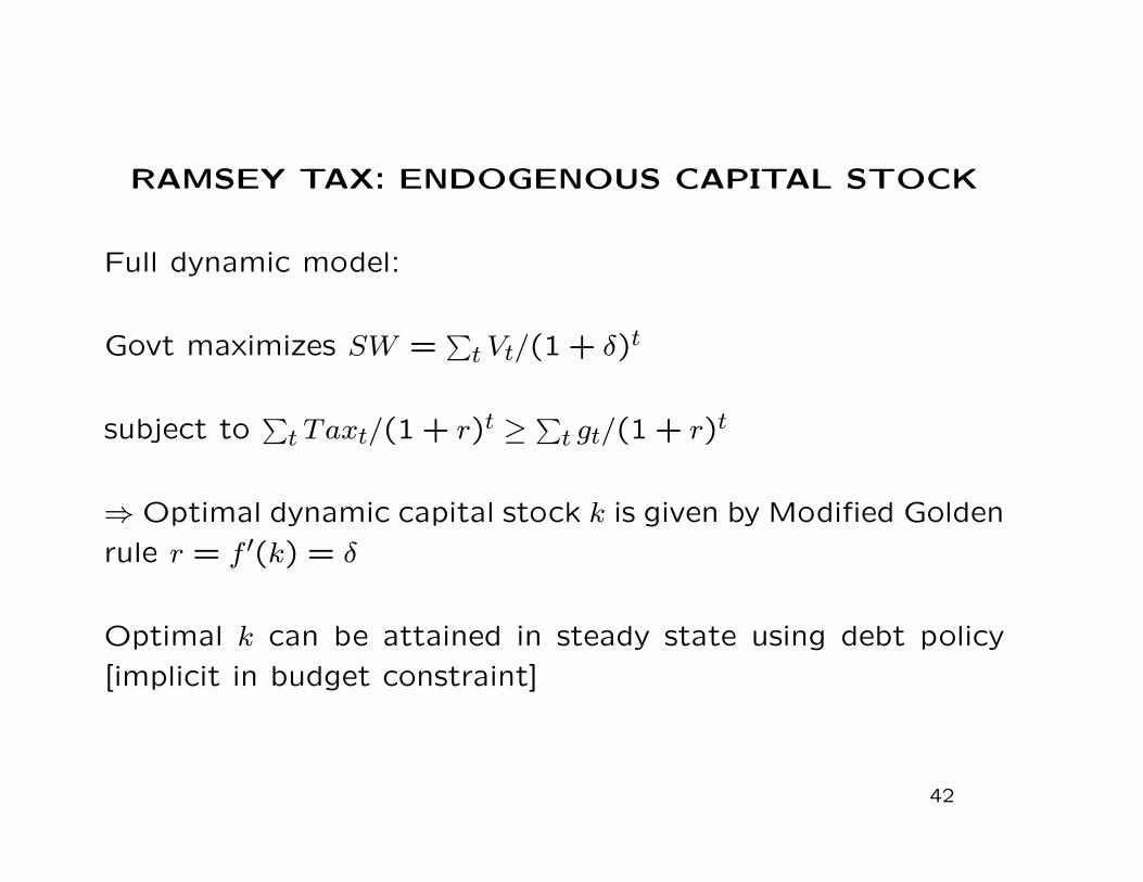
RAMSEY TAX: ENDOGENOUS CAPITAL STOCK
Full dynamic model:
Govt maximizes SW =∑t Vt/(1 + �)t
subject to∑t Taxt/(1 + r)t ≥
∑t gt/(1 + r)t
⇒Optimal dynamic capital stock k is given by Modified Golden
rule r = f ′(k) = �
Optimal k can be attained in steady state using debt policy
[implicit in budget constraint]
42

RAMSEY TAX: ENDOGENOUS CAPITAL STOCK
If the govt cannot use debt policy then optimal dynamic capital
level may not be attained because savings equal capital st = Kt⇒ tax formulas need to be modified: optimal tax rate reflect
(a) the trade-off between conventional [intra-generational] ef-
ficiency losses [static Ramsey]
(b) the failure to achieve the dynamic optimality condition on
capital stock [inter-generational efficiency trade-off]
⇒ Effect on capital tax rate level is actually ambiguous
43
RAMSEY CAPITAL INCOME TAX: REMARKS
1) No redistributive concerns: Can extend model to the multi-
person case ⇒ Higher rate �K if capital income concentrated
among the rich (Park JPubE, 1991).
2) No bequests so this model does not capture an important
aspect of wealth accumulation and justification for redistribu-
tion.
3) Only a two period model, if more periods are introduced
(as in the Auerbach-Kotlikoff simulation model), then optimal
tax formula would be more complex.
44

ATKINSON-STIGLITZ JpubE ’76
Heterogeneous individuals and government uses nonlinear tax
on earnings. Should the govt also use tax on savings?
V ℎ = maxUℎ(v(c1, c2), l) st c1+c2/(1+r(1−�K)) = wl−TL(wl)
If utility is weakly separable and v(c1, c2) is the same for all
individuals, then the government should use only labor income
tax and should not use tax on savings
Recent proof by Laroque EJ ’05 or Kaplow JpubE ’06.
Tax on savings justified if: (1) High skill people have higher
taste for saving [Saez, JpubE ’02 with calibration Golosov-
Tsyvinski-Weinzerl ’09], (2) c2 is complementary with leisure
45
RECONCILING RAMSEY AND ATKINSON-STIGLITZ
1) Ramsey model: use relative elasticities rule
r�K1 + r
(�L2 − �22) =�L
1− �L(�LL − �2L)
2) Atkinson-Stiglitz: tax only labor income when U(v(c1, c2), l)
Why are results so different across the two models?
Atkinson-Stiglitz imposes strong implicit assumptions on cross
elasticities: maxU(V ((1 − �L)wl + y, q), l) ⇒ ∂lc/∂q ∕= 0 and
loosely speaking �2L ≃ �LL
Difficult to know whether �2L ≃ 0 is better assumption than
�2L ≃ �LL
46

DIAMOND-SPINNEWIJN ’09
Heterogeneity of individuals in ability (wage rate) and discountrate. Discrete earnings choice model (high vs. low) and dis-crete discount (high vs. low) [Four type model]
Govt can tax both earnings and savings non-linearly: bi-dimensionaltax function with bi-dimensional heterogeneity
Start from no savings tax and optimal earnings tax
Result: introducing a small savings tax on high earners or asmall savings subsidy on low earners increases welfare
Intuition: Those valuing the future more (relative to the disu-tility of work) are more willing to work than those valuingthe future less ⇒ work IC constraint binds for high wage/lowsavers but not for high wage/high saver ⇒ Scope for taxingsavings
47

LIMITS OF LIFE-CYCLE MODEL
Atkinson-Stiglitz shows that life-time savings should not betaxed, tax only labor income
From justice view: seems fair to not discriminate againstsavers if labor earnings is the only source of inequality andis taxed non-linearly
In reality, capital income inequality also due
(1) difference in rates of returns
(2) shifting of labor income into capital income
(3) inheritances
(1) is not relevant if individuals handle risky assets rationally(as in CAPM model), probably not a very good assumption ⇒Tax on lucky returns might be desirable
48

SHIFTING OF LABOR / CAPITAL INCOME
In practice, difficult to distinguish between capital and laborincome [e.g., small business profits, professional traders]
Differential tax treatment can induce shifting:
(1) US C-corporations vs S-corporations: shift from corporateincome and realized capital gains toward individual businessincome [Gordon and Slemrod ’00]
(2) Carried interest in the US: hedge fund and private equityfund managers receive fraction of profits of assets they managefor clients. Those profits are really labor income but are taxedas realized capital gains
(3) Finnish Dual income tax system: taxes separately capitalincome at preferred rates since 1993: Pirtila and Selin (2007)show that it induced shifting from labor to capital incomeespecially among self-employed
49

THEORY: SHIFTING OF LABOR / CAPITAL
INCOME
Extreme case where government cannot distinguish at all be-tween labor and capital income ⇒ Govt observes only wl+ rk
⇒ Only option is to have identical MTRs at individual level ⇒General income tax Tax = T (wl + rk)
With a finite shifting elasticity, differential MTRs for labor andcapital income taxation induce an additional shifting distortion
The higher the shifting elasticity, the closer the tax rates onlabor and capital income should be [Christiansen and TuomalaITAX’08]
In practice, this seems to be a very important considerationwhen designing income tax systems [especially for top incomes]⇒ Strong reason for having �L = �K at the top
50

TAXATION OF INHERITANCES: WELFARE
EFFECTS
Definitions: donor is the person giving, donee is the person
receiving
Inheritances and inter-vivos transfers raise difficult issues:
(1) Inequality in inheritances contributes to economic inequal-
ity: seems fair to redistribute from those who received inheri-
tances to those who did not
(2) However, it seems unfair to double tax the donor who
worked hard to pass on wealth to children
⇒ Double welfare effect: inheritance tax hurts donor (if donor
altruistic to donee) and donee (which receives less)
51

TAXATION OF INHERITANCES: BEHAVIORAL
RESPONSES
Potential behavioral response effects of inheritance tax:
(1) reduces wealth accumulation of altruistic donors (and hencetax base)
(2) reduces labor supply of altruistic donors (less motivatedto work if cannot pass wealth to kids)
(3) induces donees to work more through income effects (Carnegieeffect, Holtz-Eakin,Joulfaian,Rosen QJE’93)
Critical to understand why there are inheritances to decide onoptimal inheritance tax policy. 4 main models of bequests: (a)accidental, (b) warm glow, (c) manipulative bequest motive,(d) dynastic
52
ACCIDENTAL BEQUESTS
People die with a stock of wealth they intended to spend onthemselves: Such bequests arise because of imperfect annuitymarkets
Annuity is an insurance contract converting lumpsum amountinto a stream of payments till end of life [insurance againstrisk of living too long]
Annuity markets are imperfect because of adverse selection[Finkelstein-Poterba EJ’02, JPE’04] or behavioral reasons [in-ertia, lack of planning]
Public retirement programs [and old defined benefit privatepensions] are in general annuities
Newer defined contribution private pensions [401(k)s in theUS] are in general not annuitized
53
ACCIDENTAL BEQUESTS
Bequest taxation has no distortionary effect on behavior of
donor and can only increase labor supply of donees (through
income effects) ⇒ strong case for taxing bequests heavily
Kopczuk JPE ’03 makes the point that estate tax plays the
role of a second best annuity:
Estate tax paid by those who die early, and not by those who
die late ⇒ Implicit insurance against risk of living too long
Same tax policy conclusion arises if donors have wealth in their
utility function [social status or power, Carroll ’00]
54
WARM GLOW OR ALTRUISTIC BEQUESTS
u(c)−ℎ(l)+�v(b) where c is own consumption, l is labor supply,
and b is net-of-tax bequests left to next generation and v(b)
is warm glow utility of bequests
Budget with no estate tax: c+ b/(1 + r) = wl− TL(wl)
Budget with estate tax at rate �E: c + b/[(1 + r)(1 − �E)] =
wl− TL(wl)
Suppose first that b is not bequeathed but used for “after-
life” consumption [e.g., funerary monument of no value to
next generation]
⇒ Atkinson-Stiglitz implies that b should not be taxed [�E = 0]
and that nonlinear tax on wl is enough for redistribution
55

WARM GLOW OR ALTRUISTIC BEQUESTS
Suppose now that b is given to a heir derives utility vℎeir(b)
⇒ b creates a positive externality and should be subsidized ⇒�E < 0 is optimal
Kaplow ’01 makes this point informally
Farhi-Werning QJE’10 develop formal model of non-linear Pigou-
vian subsidization of bequests with 2 generations and social
Welfare: SW =∫
[u(c)− ℎ(l) + �v(b) + vℎeir(b)]f(w)dw
The marginal external effect of bequests is dvℎeir/db and hence
should be smaller for large b
⇒ Optimal subsidy is smaller for large estates ⇒ progressive
estate subsidy
56

WARM GLOW BEQUESTS: ISSUES
(a) If past inheritances come from untaxed labor income, then
it is desirable to tax inheritances [important when income tax
starts]
(b) Double counting issue: should social welfare double count
bequests? [both for donor and donee]
Yes under utilitarian framework [Kaplow ’01]
No: utilitarian framework with double counting generates pre-
dictions that conflict with horizontal equity:
∙ Govt should tax less those well loved by other people
∙ Govt should care more about kids with parents than orphans
57

MANIPULATIVE BEQUESTS
Parents use potential bequest to extract favors from children
Empirical Evidence: Bernheim-Shleifer-Summers JPE ’85 show
that number of visits of children to parents is correlated with
bequeathable wealth but not annuitized wealth of parents
⇒ Bequest becomes one additional form of labor income for
donee and one consumption good for donor
⇒ Inheritances should be counted and taxed as labor income
for donees
58

SOCIAL-FAMILY PRESSURE BEQUESTS
Parents may not want to leave bequests but feel compelledto by pressure of heirs or society: bargaining between parentsand children
With estate tax, parents do not feel like they need to give asmuch ⇒ parents are made better-off by the estate tax ⇒ Casefor estate taxation stronger [Atkinson-Stiglitz does not applyand no double counting of bequests]
Empirical evidence:
Aura JpubE’05: reform of private pension annuities in theUS in 1984 requiring both spouses signatures when workerdecides to get a single annuity or couple annuity: reform ↑sharply couple annuities choice
Equal division of estates [Wilhelm AER’96, McGarry]: estatesare very often divided equally but gifts are not
59
DYNASTIC MODEL OR INFINITE HORIZON
Special case of warm glow: Vt = u(ct, lt) + �Vt+1 implies
V0 =∑t
�tu(ct, lt)
st∑t ct/(1 + r)t ≤
∑twtlt/(1 + r)t
Dynasty with Ricardian equivalence: consumption dependsonly on PDV of earnings of dynasty
Poor empirical fit:
1) Altonji-Hayashi-Kotlikoff AER’92, JPE’97 show that in-come shocks to parents have bigger effect on parents con-sumption than on kids consumption
2) Temporary tax cut debt financed [fiscal stimulus] shouldhave no impact on consumption
60

INFINITE HORIZON MODEL: CHAMLEY-JUDD
Infinite horizon with no uncertainty. Govt can collect taxesusing labor income tax or capital income taxes (but cannotconfiscate initial wealth which would be optimal) that varyperiod by period
V0 =∑t
u(ct, lt)/(1 + �)t
st∑t qtct ≤
∑t qtwt(1− � tL)lt +A0 (�)
q0 = 1, q1 = 1/(1+r1(1−�1K), ..., qt = 1/
∏ts=1(1+rs(1−�sK))
FOC in lt and ct ⇒ wt(1 − � tL)utc − utl = 0, ut+1c /utc = (1 +
�)/(1 + r(1− � tK))
With constant tax rate �K and constant r: Before tax price:pt = 1/(1 + r)t and after-tax price qt = 1/(1 + r(1− �K))t ⇒
Price distortion qt/pt grows exponentially with time
61

CHAMLEY-JUDD: RESULTS
Chamley-Judd show that the capital income tax rate always
tends to zero asymptotically: no capital tax in the long-run.
This is due to 2 reasons, each of which is actually sufficient:
(1) Infinite supply elasticity of the capital stock k with respect
to the net-of-tax rate of return r(1− �K)
(2) Government objective maximizes welfare of the dynasty
seen from the first generation [V0 objective]
62

CHAMLEY-JUDD, INFINITE ELASTICITY
Two classes: capitalists save as in infinite horizon model,workers do not save (consume wages w with no labor sup-ply effects)
Can capital tax at rate � be desirable for workers in steady-state?
r = f ′(k) and w = f(k)−kf ′(k), tax � , net return is (1−�)f ′(k)
Infinite horizon: modified Golden rule: discount rate � = (1−�)f ′(k) (if >, save more and k increases, if <, save less and kdecreases).
Workers get w + f ′(k)�k = f(k) − (1 − �)kf ′(k) = f(k) − �k,maximized when f ′(k) = �, ie � = 0
Intuition: Supply of k is infinitely elastic: taxing an infinitelyelastic good cannot be desirable [even in the steady state]
63

CHAMLEY-JUDD, V0 objective
It is possible to build a model with endogenous discount rate
�(c) so that elasticity of k stock with respect to long-term
return r is finite
Judd JpubE ’85 shows that:
If workers have the same discount rate as capitalists (asymp-
totically) then long-run zero capital income tax result carries
over
This is about inter-temporal distortions: a constant capital
income tax rate �K produces a growing distortion overtime
while Ramsey recommends to spread taxes across goods
64
ISSUES IN INFINITE HORIZON MODEL
1) Taxing initial wealth would be most efficient [as this would
be lumpsum taxation]
2) Chamley-Judd tax is not time consistent: the government
would like to renege and start taxing capital again
3) Zero-long run tax result is not robust to using progressive
income taxation [Piketty, ’01, Saez ’02]
4) Dynastic model requires strong homogeneity assumptions
(in discount rates) to generate reasonable steady states [un-
likely to hold in practice]
Bottom line: Not very useful model for thinking about capital
income taxation65
PROGRESSIVE TAX IN ∞ HORIZON: PIKETTY ’01
Dynastic utilities with inelastic labor supply
W =∑t
u(ct)/(1 + �)t
rt = f ′(kt), wt = f(kt)− rtkt
Distribution of wealth: at with density ft(at) so that kt =∫agt(a)da
Golden rule capital stock k∗: f ′(k∗) = �
With no taxes: In steady state: f ′(k∞) = � (i.e k∞ = k∗), anyg∞(a) possible as long as k∗ =
∫ag∞(a)da
Proof: suppose r∞ = f ′(k∞) > � ⇒ u′(ct+1)/u(ct) = (1 +�)/(1 + rt) < 1 i.e., ct+1 > ct ⇒ Individuals want to shift con-sumption toward future ⇒ Save more and accumulate capitalindefinitely [not a steady state]
66
PROGRESSIVE TAX IN ∞ HORIZON: PIKETTY ’01
Suppose a progressive capital income tax is introduced: �K =
0 when a ≤ k̄ and �K = � > 0 when a ≥ k̄
Assume k̄ > k∗
In the steady state:
1) Golden rule capital stock: k∞ =∫ag∞(a)da = k∗
2) Truncated wealth distribution: a ≤ k̄ for all individuals
Proof: In steady state, all individuals must face same net-of-
tax rate r∞(1−�K) ⇒ All individuals in same tax bracket [0, k̄]
or (k̄,∞). But (k̄,∞) is impossible because k∞ =∫ag(a)da ≥
k̄ > k∗ and hence f ′(k∞) < �
67
PROGRESSIVE TAX IN ∞ HORIZON: SAEZ ’02
Piketty ’01 shows that progressive capital income tax with
exemption up to k∗ equalizes wealth without affecting long-
run capital stock
Seems desirable from steady-state perspective
Saez ’02 shows that such progressive taxation is desirable from
period 0 perspective if
a ⋅� < 1 where a is Pareto parameter of initial wealth distribu-
tion and � is inter-temporal elasticity of substitution u(ct) =
[c1−1/�t − 1]/[1− 1/�]
Long-run wealth distribution will then be truncated
68

MAKING PROGRESS IN OPTIMAL CAPITAL
INCOME THEORY
Ideal research plan:
1) Develop tax formulas that are based on sufficient statistics
that can be estimated empirically [behavioral responses and
distributive factors]
2) Formulas should be robust to heterogeneity in preferences
[accidental, warm glow, dynastic, manipulative]
3) Predictions from theory should be somewhat aligned to
actual practice [taxing only earnings and not at all capital
does not fit with actual practice]
4) Progress may require to deviate from utilitarian criterion
69
NEW DYNAMIC PUBLIC FINANCE: REFERENCES
Dynamic taxation in the presence of future earnings uncer-
tainty
Recent series of papers following upon on Golosov, Kocher-
lakota, Tsyvinski REStud ’03 (GKT)
Principle can be understood in 2 period model: Diamond-
Mirrlees JpubE ’78 and Cremer-Gahvari EJ ’95
Generalized to many periods by GKT and subsequent papers
Simple exposition is Kocherlakota AER-PP ’04
Two comprehensive surveys: Golosov-Tsyvinski-Werning ’06
and Kocherlakota ’10 book70

NEW DYNAMIC PUBLIC FINANCE
Key ingredient is uncertainty in future ability w
2 period simple model:
(0) Everybody is identical in period 0: no work and consume
c0, period 0 utility is u(c0)
(1) Ability w revealed in period 1, work l and earn z = wl,
consume c1, period 1 utility u(c1)− ℎ(l)
Total utility u(c0) + �[u(c1)− ℎ(l)]
Rate of return r, gross return R = 1 + r
Discount rate � < 1
71
STANDARD EULER EQUATION
No govt intervention: c0 + c1/R = wl/R
Solve model backward (assume c0 given):
Period 1: c1 = wl−Rc0, choose l to maximize u(wl−Rc0)−ℎ(l)
⇒ FOC wu′(wl−Rc0) = ℎ′(l) ⇒ l∗ = l(w, c0)
Period 0: Choose c0 to maximize: u(c0) + �∫
[u(wl∗ − Rc0) −ℎ(l∗)]f(w)dw
FOC for c0 (using envelope condition for l∗)
u′(c0) = �R∫u′(c1)f(w)dw
This is called the Euler equation
72
MECHANISM DESIGN
Government would like to redistribute from high w to low w.
Government does not observe w but can observe c0, c1, z = wl
and can set taxes as a function of c0, c1, z
Equivalently (using revelation principle), govt can offer menu
(c0, c1(w), z(w))w and let individuals truthfully reveal their w
Govt program: choose menu (c0, c1(w), z(w))w to maximize:
SW = u(c0) + �∫
[u(c1(w))− ℎ(z(w)/w)]f(w)dw st
1) Budget: c0 +∫c1(w)f(w)dw/R ≤
∫z(w)f(w)dw/R
2) Incentive Compatibility (IC): individual w prefers c0, c1(w), z(w)
to any other c0, c1(w′), z(w′)
73

INVERSE EULER EQUATION
Inverse Euler equation holds at the govt optimum:
1
u′(c0)=
1
�R⋅∫ 1
u′(c1(w))f(w)dw
Proof: small deviation in menus offered: ∆c0 = −"/u′(c0) and∆c1(w) = "/[�u′(c1(w))]
Does not affect individual utilities in any state:
u(c0 + ∆c0) + �u(c1(w) + ∆c1(w)) = u(c0) + �u(c1(w)) +∆c0u
′(c0) + ∆c1(w)�u′(c1(w)) = u(c0) + �u(c1(w))
⇒ (IC) continues to hold and SW unchanged
⇒ If deviation creates a surplus (or deficit) in govt budget,then initial menu not optimal ⇒ Deviation must be budgetneutral ⇒ −"/u′(c0) +
∫"f(w)dw/[�Ru′(c1(w))] = 0
74
INTERTEMPORAL WEDGE
Jensen Inequality ⇒ K(∫x(w)dF (w)) <
∫K(x(w))dF (w) for
K(.) convex
Apply this to K(x) = 1/x and x(w) = u′(c1(w)) ⇒
1∫u′(c1(w))f(w)dw
<∫
f(w)dw
u′(c1(w))=
�R
u′(c0)
⇒ u′(c0) < �R∫u′(c1(w))f(w)dw
⇒ Optimal govt redistribution imposes a positive tax wedge
on intertemporal choice
75
DECENTRALIZATION AND INTUITION
Decentralization: Optimum can be decentralized with a taxon capital income [which depends on current labor income]along with a nonlinear tax on wage income [KocherlakotaEMA’06]
Economic intuition: If high skill person works less (to imitatelower skill person), person would also like to reduce c0 andhence save more, so tax on savings is a good way to discourageimitation
Result depends crucially on rationality in inter-temporal choices,not clear yet how applicable this is in practice
Golosov-Tsyvinski JPE’04 present decentralization results inthe case of disability insurance (generalizing Diamond-MirrleesJpubE ’78): govt imposes an asset test on recipients
76