14.452 Fall 2016 Lecture 8: Neoclassical …...November 22, 2016. 1 / 42 14.452 Economic Growth: Lecture 8, Neoclassical Endogenous Growth Daron Acemoglu MIT November 22, 2016. First-Generation

Daron Acemoglu (MIT) Economic Growth Lecture 8 November 22, 2016. 1 / 42

14.452 Economic Growth: Lecture 8, NeoclassicalEndogenous Growth

Daron Acemoglu

MIT

November 22, 2016.

First-Generation Models of Endogenous Growth

Models so far: no sustained long-run growth; relatively little to sayabout sources of technology differences.Models in which technology evolves as a result of firms’and workers’decisions are most attractive in this regard.But sustained economic growth is possible in the neoclassical modelas well:

AK model before: relaxed Assumption 2 and prevented diminishingreturns to capital.Capital accumulation could act as the engine of sustained economicgrowth.

Neoclassical version of the AK model:Very tractable and applications in many areas.Shortcoming: capital is essentially the only factor of production,asymptotically share of income accruing to it tends to 1.

Two-sector endogenous growth models behave very similarly to thebaseline AK model, but avoid this.


Demographics, Preferences and Technology I

Focus on balanced economic growth, i.e. consistent with the Kaldorfacts.

Thus CRRA preferences as in the canonical neoclassical growth model.

Economy admits an infinitely-lived representative household,household size growing at the exponential rate n.

Preferences

U =∫ ∞

exp (0

− (ρ− n) t)[c (t 1) −θ − 11− θ

]dt. (1)

Labor is supplied inelastically.

Flow budget constraint,

a (t) = (r (t)− n)a (t) + w (t)− c (t) , (2)


Demographics, Preferences and Technology II

No-Ponzi game constraint:{ [ ∫ tlim a(t) expt→∞

− [r(s)0

− n] ds]}≥ 0. (3)

Euler equation:c (t)c (t)

=1θ(r (t)− ρ). (4)

Transversality condition,

limt→∞

{a(t) exp

[−∫ t[r(s)

0− n] ds

]}= 0. (5)

Problem is concave, solution to these necessary conditions is in factan optimal plan.Final good sector similar to before, but Assumptions 1 and 2 are notsatisfied.


Demographics, Preferences and Technology III

More specifically,Y (t) = AK (t) ,

with A > 0.

Does not depend on labor, thus w (t) in (2) will be equal to zero.

Defining k (t) ≡ K (t) /L (t) as the capital-labor ratio,

Y (t)y (t) ≡

L (t)= Ak (t) . (6)

Notice output is only a function of capital, and there are nodiminishing returns

But introducing diminishing returns to capital does not affect themain results in this section.


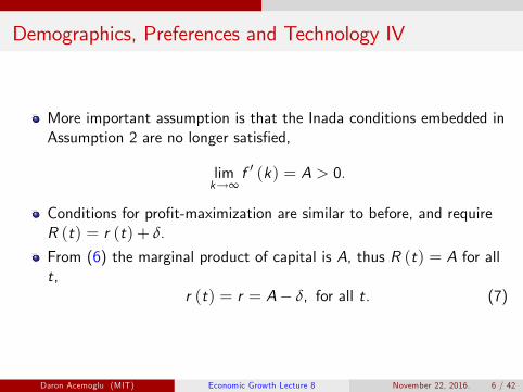
Demographics, Preferences and Technology IV

More important assumption is that the Inada conditions embedded inAssumption 2 are no longer satisfied,

lim f ′ (k) = A > 0.k→∞

Conditions for profit-maximization are similar to before, and requireR (t) = r (t) + δ.

From (6) the marginal product of capital is A, thus R (t) = A for allt,

r (t) = r = A− δ, for all t. (7)


Equilibrium I

A competitive equilibrium of this economy consists of paths[c (t) , k (t ∞) ,w (t) ,R (t)]t=0, such that the representative householdmaximizes (1) subject to (2) and (3) given initial capital-labor ratiok (0) and [w (t ∞) , r (t)]t=0 such that w (t) = 0 for all t, and r (t) isgiven by (7).

Note that a (t) = k (t).

Using the fact that r = A− δ and w = 0, equations (2), (4), and (5)imply

k (t) = (A− δ− n)k (t)− c (t) (8)

c (t) 1= (A− δ− ρ), (9)

c (t) θ

lim k(t) exp (t→∞

−(A− δ− n)t) = 0. (10)


Equilibrium II

The important result immediately follows from (9).

Since the right-hand side is constant, there must be a constant rate ofconsumption growth (as long as A− δGrowth of consumption is independent

− ρ > 0).of the level of capital stock per

person, k (t).No transitional dynamics in this model.

To develop, integrate (9) starting from some c(0), to be determinedfrom the lifetime budget constraint,

1c(t) = c(0) exp

((A

θ− δ− ρ)t

). (11)

Need to ensure that the transversality condition is satisfied and ensurepositive growth (A− δ− ρ > 0). Impose:

A > ρ+ δ > (1 θ) (A δ) + θn+ δ. (12)− −


Equilibrium Characterization

Equilibrium Characterization I

No transitional dynamics: growth rates of consumption, capital andoutput are constant and given in (9).

Substitute for c(t) from equation (11) into equation (8),

1k (t) = (A− δ− n)k (t)− c(0) exp

((A

θ− δ− ρ)t

), (13)

First-order, non-autonomous linear differential equation in k (t).Recall that if

z (t) = az (t) + b (t) ,

then, the solution is

tz (t) = z0 exp (at) + exp (at)

∫exp (−as) b(s)ds,

0

for some constant z0 chosen to satisfy the boundary conditions.



Equilibrium Characterization II

Therefore, equation (13) solves for:

κ exp((A δ n) t) + (A δ)(θ 1)θ−1 1+ ρθ− n−1

k(t) =

{− −

[− − −

,×[c(0) exp

(θ−1(A− δ− ρ)t

] })](14)

where κ is a constant to be determined.Assumption (12) ensures that

(A− δ)(θ − 1)θ−1 + ρθ−1 − n > 0.Substitute from (14) into the transversality condition, (10),[ −1 1 1

0 = lim [κ + (A− δ)(θ − 1)θ + ρθ−t ∞

− n −→

×

c 1(0) exp(−(A− 1δ)(θ − 1)θ− + ρθ− −

]n)t)].

Since (A− δ)(θ − 1)θ−1 + ρθ−1 − n > 0, the second term in thisexpression converges to zero as t → ∞.



Equilibrium Characterization III

But the first term is a constant.

Thus the transversality condition can only be satisfied if κ = 0.

Therefore we have from (14) that:

1k(t) = (A− 1 1δ)(θ − 1)θ− + ρθ− − n − (15)

[× c

][(0) exp

(θ−1(A δ ρ)t

k 0 exp( −1 − −

= ( ) θ (A− δ− ρ)t ,

)])Second line follows from the fact that the boundary condition has tohold for capital at t = 0. T

Hence capital and output grow at the same rate as consumption.

This also pins down the initial level of consumption as

c (0) =[(A− 1 1δ)(θ − 1)θ− + ρθ− − n

]k (0) . (16)



Equilibrium Characterization IV

Growth is not only sustained, but also endogenous in the sense ofbeing affected by underlying parameters.

E.g., an increase in ρ, will reduce the growth rate.

Saving rate=total investment (increase in capital plus replacementinvestment) divided by output:

K (t) + δK (t)s =

Y (t)

k (t) /k (t) + n+ δ=

AA

=− ρ+ θn+ (θ − 1)δ

, (17)θA

Last equality exploited k (t) /k (t) = (A− δ− ρ)/θ.



Equilibrium Characterization V

Saving rate, constant and exogenous in the basic Solow model, isagain constant.

But is now a function of parameters, also those that determine theequilibrium growth rate of the economy.

Proposition Consider the above-described AK economy, with arepresentative household with preferences given by (1), andthe production technology given by (6). Suppose thatcondition (12) holds. Then, there exists a unique equilibriumpath in which consumption, capital and output all grow atthe same rate g ∗ ≡ (A− δ− ρ)/θ > 0 starting from anyinitial positive capital stock per worker k (0), and the savingrate is endogenously determined by (17).



Equilibrium Characterization VI

Since all markets are competitive, there is a representative household,and there are no externalities, the competitive equilibrium will bePareto optimal.

Can be proved either using First Welfare Theorem type reasoning, orby directly constructing the optimal growth solution.

Proposition Consider the above-described AK economy, with arepresentative household with preferences given by (1), andthe production technology given by (6). Suppose thatcondition (12) holds. Then, the unique competitiveequilibrium is Pareto optimal.


The Role of Policy

The Role of Policy I

Suppose there is an effective tax rate of τ on the rate of return fromcapital income, so budget constraint becomes:

a (t) = ((1− τ) r (t)− n)a (t) + w (t)− c (t) . (18)

Repeating the analysis above this will adversely affect the growth rateof the economy, now:

(1g =

− τ) (A− δ)− ρ

θ. (19)

Moreover, saving rate will now be

(1− τ)As =

− ρ+ θn− (1− τ − θ) δ, (20)

θA

which is a decreasing function of τ if A− δ > 0.


The Role of Policy

The Role of Policy II

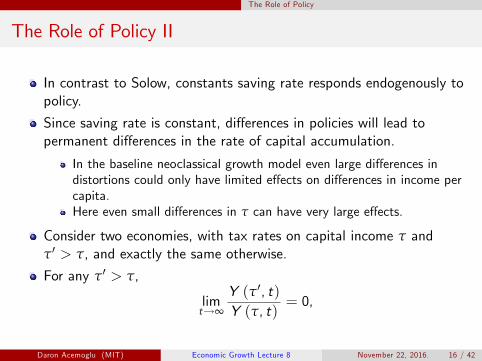
In contrast to Solow, constants saving rate responds endogenously topolicy.

Since saving rate is constant, differences in policies will lead topermanent differences in the rate of capital accumulation.

In the baseline neoclassical growth model even large differences indistortions could only have limited effects on differences in income percapita.Here even small differences in τ can have very large effects.

Consider two economies, with tax rates on capital income τ andτ′ > τ, and exactly the same otherwise.

For any τ′ > τ,Y (τ′, t)

limt→∞ Y (τ, t)

= 0,


The Role of Policy

The Role of Policy III

Why then focus on standard neoclassical if AK model can generatearbitrarily large differences?

1 AK model, with no diminishing returns and the share of capital innational income asymptoting to 1, is not a good approximation toreality.

2 Relative stability of the world income distribution in the post-war eramakes it more attractive to focus on models in which there is astationary world income distribution.


The Two-Sector AK Model The Rebelo Model

The Two-Sector AK Model I

Model before creates another factor of production that accumulateslinearly, so equilibrium is again equivalent to the one-sector AKeconomy.

Thus, in some deep sense, the economies of both sections areone-sector models.

Also, potentially blur key underlying characteristic driving growth.

What is important is not that production technology is AK , but thatthe accumulation technology is linear.

Preference and demographics are the same as in the model of theprevious section, (1)-(5) apply as before

No population growth, i.e., n = 0, and L is supplied inelastically.

Rather than a single good used for consumption and investment, nowtwo sectors.



The Two-Sector AK Model II

Sector 1 produces consumption goods with the following technology

C (t 1) = B (KC (t))α LC (t)

−α , (21)

Cobb-Douglas assumption here is quite important in ensuring that theshare of capital in national income is constant

Capital accumulation equation:

K (t) = I (t)− δK (t) ,

I (t) denotes investment. Investment goods are produced with adifferent technology,

I (t) = AKI (t) . (22)

Extreme version of an assumption often made in two-sector models:investment-good sector is more capital-intensive than theconsumption-good sector.



The Two-Sector AK Model III

Market clearing implies:

KC (t) +KI (t) ≤ K (t),

LC (t) ≤ L,An equilibrium is defined similarly, but also features an allocationdecision of capital between the two sectors.Also, there will be a relative price between the two sectors which willadjust endogenously.Both market clearing conditions will hold as equalities, so letting κ (t)denote the share of capital used in the investment sector

KC (t) = (1− κ (t))K (t) and KI (t) = κ (t)K (t).

From profit maximization, the rate of return to capital has to be thesame when it is employed in the two sectors.



The Two-Sector AK Model IV

Let the price of the investment good be denoted by pI (t) and that ofthe consumption good by pC (t), then

LpI (t)A = pC (t) αB

((1− κ (t))K (t)

)1−α

. (23)

Define a steady-state (a balanced growth path) as an equilibrium pathin which κ (t) is constant and equal to some κ ∈ [0, 1].Moreover, choose the consumption good as the numeraire, so thatpC (t) = 1 for all t.

Then differentiating (23) implies that at the steady state:

pI (t) =pI (t)

− (1− α) gK , (24)

gK is the steady-state (BGP) growth rate of capital.



The Two-Sector AK Model V

Euler equation (4) still holds, but interest rate has to be forconsumption-denominated loans, rC (t).

I.e., the interest rate that measures how many units of consumptiongood an individual will receive tomorrow by giving up one unit ofconsumption today.

Relative price of consumption goods and investment goods ischanging over time, thus:

By giving up one dollar, the individual will buy 1/pI (t) units of capitalgoods.This will have an instantaneous return of rI (t).Individual will get back the one unit of capital, which has experienced achange in its price of pI (t) /pI (t).Finally, he will have to buy consumption goods, whose prices changedby pC (t) /pC (t).



The Two-Sector AK Model VI

Therefore,r

rC (tI (t)

) =pI (t)

+pI (t) ppI (t)

− C (t). (25)

pC (t)

Given our choice of numeraire, we have pC (t) /pC (t) = 0.Moreover, pI (t) /pI (t) is given by (24).Finally,

rI (t) = ApI (t)

− δ

given the linear technology in (22).

Therefore, we have

prC (t) = A− I (t)

δ+pI (t)

.



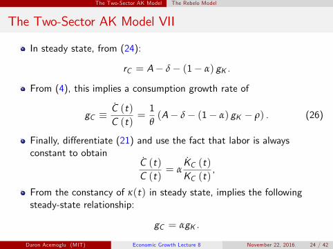
The Two-Sector AK Model VII

In steady state, from (24):

rC = A− δ− (1− α) gK .

From (4), this implies a consumption growth rate of

C (t)gC ≡ C (t)

=1θ(A− δ− (1− α) gK − ρ) . (26)

Finally, differentiate (21) and use the fact that labor is alwaysconstant to obtain

C (t)C (t)

= αKC (t)KC (t)

,

From the constancy of κ(t) in steady state, implies the followingsteady-state relationship:

gC = αgK .



The Two-Sector AK Model VIII

Substituting this into (26), we have

AgK∗ =

− δ− ρ(27)

1− α (1− θ)

andA

gC∗ = α

− δ− ρ

1− α (1− θ). (28)

Because labor is being used in the consumption good sector, therewill be positive wages.

Since labor markets are competitive,((1− κ (t))K (t)

w (t) = (1− α) pC (t)B L

)α

.



The Two-Sector AK Model IX

Therefore, in the balanced growth path,

w (t) pC (t)=w (t) pC (t)

+ αK (t)K (t)

= αgK∗ ,

Thus wages also grow at the same rate as consumption.

Proposition In the above-described two-sector neoclassical economy,starting from any K (0) > 0, consumption and labor incomegrow at the constant rate given by (28), while the capitalstock grows at the constant rate (27).

Can do policy analysis as before



The Two-Sector AK Model X

Different from the neoclassical growth model, there is continuouscapital deepening.

Capital grows at a faster rate than consumption and output. Whetherthis is a realistic feature is debatable:

Kaldor facts include constant capital-output ratio as one of therequirements of balanced growth.For much of the 20th century, capital-output ratio has been constant,but it has been increasing steadily over the past 30 years.Part of the increase is because of relative price adjustments that haveonly been performed in the recent past.


Growth with Externalities The Romer Model

Growth with Externalities I

Romer (1986): model the process of “knowledge accumulation”.

Diffi cult in the context of a competitive economy.

Solution: knowledge accumulation as a byproduct of capitalaccumulation.

Technological spillovers: arguably crude, but captures that knowledgeis a largely non-rival good.

Non-rivalry does not imply knowledge is also non-excludable.

But some of the important characteristics of “knowledge”and its rolein the production process can be captured in a reduced-form way byintroducing technological spillovers.



Preferences and Technology I

No population growth (we will see why this is important).

Production function with labor-augmenting knowledge (technology)that satisfies Assumptions 1 and 2.

Instead of working with the aggregate production function, assumethat the production side of the economy consists of a set [0, 1] offirms.

The production function facing each firm i ∈ [0, 1] is

Yi (t) = F (Ki (t) ,A (t) Li (t)) , (29)

Ki (t) and Li (t) are capital and labor rented by a firm i .

A (t) is not indexed by i , since it is technology common to all firms.



Preferences and Technology II

Normalize the measure of final good producers to 1, so marketclearing conditions: ∫ 1

Ki (t) di = K (t)0

and ∫ 1Li (t) di = L,

0

L is the constant level of labor (supplied inelastically) in this economy.

Firms are competitive in all markets, thus all hire the same capital toeffective labor ratio, and

∂F (K (t) ,A (t) L)w (t) =

∂L∂F (K (t) ,A (t) L)

R (t) = .∂K (t)



Preferences and Technology III

Key assumption: firms take A (t) as given, but this stock oftechnology (knowledge) advances endogenously for the economy as awhole.Lucas (1988) develops a similar model, but spillovers work throughhuman capital.Extreme assumption of suffi ciently strong externalities such that A (t)can grow continuously at the economy level. In particular,

A (t) = BK (t) , (30)

Motivated by “learning-by-doing.”Alternatively, could be a functionof the cumulative output that the economy has produced up to now.Substituting for (30) into (29) and using the fact that all firms arefunctioning at the same capital-effective labor ratio, productionfunction of the representative firm:

Y (t) = F (K (t) ,BK (t) L) .



Preferences and Technology IV

Using the fact that F (·, ·) is homogeneous of degree 1, we have

Y (t)= F (1,BL)

K (t)

= f (L) .

Output per capita can therefore be written as:

Y (t)y (t) ≡

LY (t)

=K (t)

K (t)L

= k (t) f (L) ,

Again k (t) ≡ K (t) /L is the capital-labor ratio in the economy.



Preferences and Technology V

Normalized production function, now f (L).

We havew (t) = K (t) f ′ (L) (31)

andR (t) = R = f (L)− Lf ′ (L) , (32)

which is constant.


Growth with Externalities Equilibrium

Equilibrium I

An equilibrium is defined as a path [C (t) ,K (t ∞)]t=0 that maximizethe utility of the representative household and [w (t) ,R (t ∞)]t=0 thatclear markets.

Important feature is that because the knowledge spillovers areexternal to the firm, factor prices are given by (31) and (32).

I.e., they do not price the role of the capital stock in increasing futureproductivity.

Since the market rate of return is r (t) = R (t)− δ, it is alsoconstant.

Usual consumer Euler equation (e.g., (4) above) then implies thatconsumption must grow at the constant rate,

1gC∗ =

θ

(f (L)− Lf ′ (L)− δ− ρ

). (33)



Equilibrium II

Capital grows exactly at the same rate as consumption, so the rate ofcapital, output and consumption growth are all gC

∗ .

Assume thatf (L)− Lf ′ (L)− δ− ρ > 0, (34)

so that there is positive growth.

But also that growth is not fast enough to violate the transversalitycondition,

(1− θ)(f (L)− Lf ′ (L)− δ

)< ρ. (35)

Proposition Consider the above-described Romer model with physicalcapital externalities. Suppose that conditions (34) and (35)are satisfied. Then, there exists a unique equilibrium pathwhere starting with any level of capital stock K (0) > 0,capital, output and consumption grow at the constant rate(33).



Equilibrium III

Population must be constant in this model because of the scale effect.

Since f (L)− Lf ′ (L) is always increasing in L (by Assumption 1), ahigher population (labor force) L leads to a higher growth rate.

The scale effect refers to this relationship between population and theequilibrium rate of economic growth.

If population is growing, the economy will not admit a steady stateand the growth rate of the economy will increase over time (outputreaching infinity in finite time and violating the transversalitycondition).


Growth with Externalities Pareto Optimal Allocations

Pareto Optimal Allocations I

Given externalities, not surprising that the decentralized equilibrium isnot Pareto optimal.

The per capita accumulation equation for this economy can bewritten as

k (t) = f (L) k (t)− c (t)− δk (t) .

The current-value Hamiltonian to maximize utility of therepresentative household is

c (t 1) −θ − 1H (k, c , µ) = + µ

1− θ

[f (L) k (t)− c (t)− δk (t)

],



Pareto Optimal Allocations II

Conditions for a candidate solution

Hc (k, c, µ) = c (t)−θ − µ (t) = 0

Hk (k, c, µ) = µ (t) f (L)− δ = −µ (t) + ρµ (t) ,

lim [exp (−ρt) µ (t) k (t)] = 0.t→∞

[ ]

H strictly concave, thus these conditions characterize unique solution.



Pareto Optimal Allocations III

Social planner’s allocation will also have a constant growth rate forconsumption (and output) given by

gS1

C = θ

(f (L)− δ− ρ ,

which is always greater than gC∗ as given by (

)33)– since

f (L) > f (L)− Lf ′ (L).Social planner takes into account that by accumulating more capital,she is improving productivity in the future.

Proposition In the above-described Romer model with physical capitalexternalities, the decentralized equilibrium is Paretosuboptimal and grows at a slower rate than the allocationthat would maximize the utility of the representativehousehold.


Conclusions Conclusions

Conclusions I

Linearity of the models (most clearly visible in the AK model):

Removes transitional dynamics and leads to a more tractablemathematical structure.Essential feature of any model that will exhibit sustained economicgrowth.With strong concavity, especially consistent with the Inada, sustainedgrowth will not be possible.

But most models studied in this chapter do not feature technologicalprogress:

Debate about whether the observed total factor productivity growth ispartly a result of mismeasurement of inputs.Could be that much of what we measure as technological progress is infact capital deepening, as in AK model and its variants.


Conclusions Conclusions

Conclusions II

Important tension:

neoclassical growth model (or Solow growth model) have diffi culty ingenerating very large income differencesmodels here suffer from the opposite problem.Both a blessing and a curse: also predict an ever expanding worlddistribution.

Issues to understand:1 Era of divergence is not the past 60 years, but the 19th century:important to confront these models with historical data.

2 “Each country as an island”approach is unlikely to be a goodapproximation, much less so when we endogenize technology.


MIT OpenCourseWarehttps://ocw.mit.edu

14.452 Economic Growth Fall 2016

For information about citing these materials or our Terms of Use, visit: https://ocw.mit.edu/terms.

https://ocw.mit.edu/terms

https://ocw.mit.edu

Documents

14.452 Fall 2016 Lecture 8: Neoclassical …...November 22, 2016. 1 / 42 14.452 Economic Growth: Lecture 8, Neoclassical Endogenous Growth Daron Acemoglu MIT November 22, 2016. First-Generation