13granger

8/6/2019 13granger

http://slidepdf.com/reader/full/13granger 1/19

Granger Causality Testing

Jamie Monogan

Washington University in St. Louis

November 10, 2010

Jamie Monogan (WUStL) Granger Causality Testing November 10, 2010 1 / 19

8/6/2019 13granger


Objectives

By the end of this meeting, participants should be able to:

Explain why F -ratios are useful in instances of multicollinearpredictors.

Conduct a direct Granger test between two variables.


8/6/2019 13granger


Background on Multicollinearity

Example

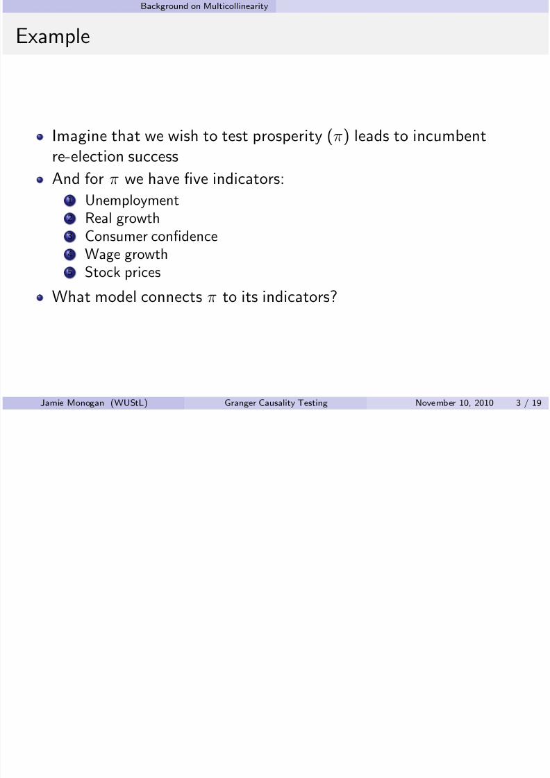
Imagine that we wish to test prosperity (π) leads to incumbentre-election success

And for π we have five indicators:1 Unemployment2 Real growth3 Consumer confidence4 Wage growth5 Stock prices

What model connects π to its indicators?


8/6/2019 13granger



The Common Factor Variance Decomposition

The variance of any indicator x of the latent concept π consists of:1 Common variance, indicating π2

Unique variance, due to the indicator itself 3 Error variance

σ2total = σ2

common + σ2unique + σ2

error

This is the theory behind measurement models such as exploratory orconfirmatory factor analysis.


B k d M l i lli i

8/6/2019 13granger



Variance Decomposition Model


8/6/2019 13granger



8/6/2019 13granger



The Error in Inference

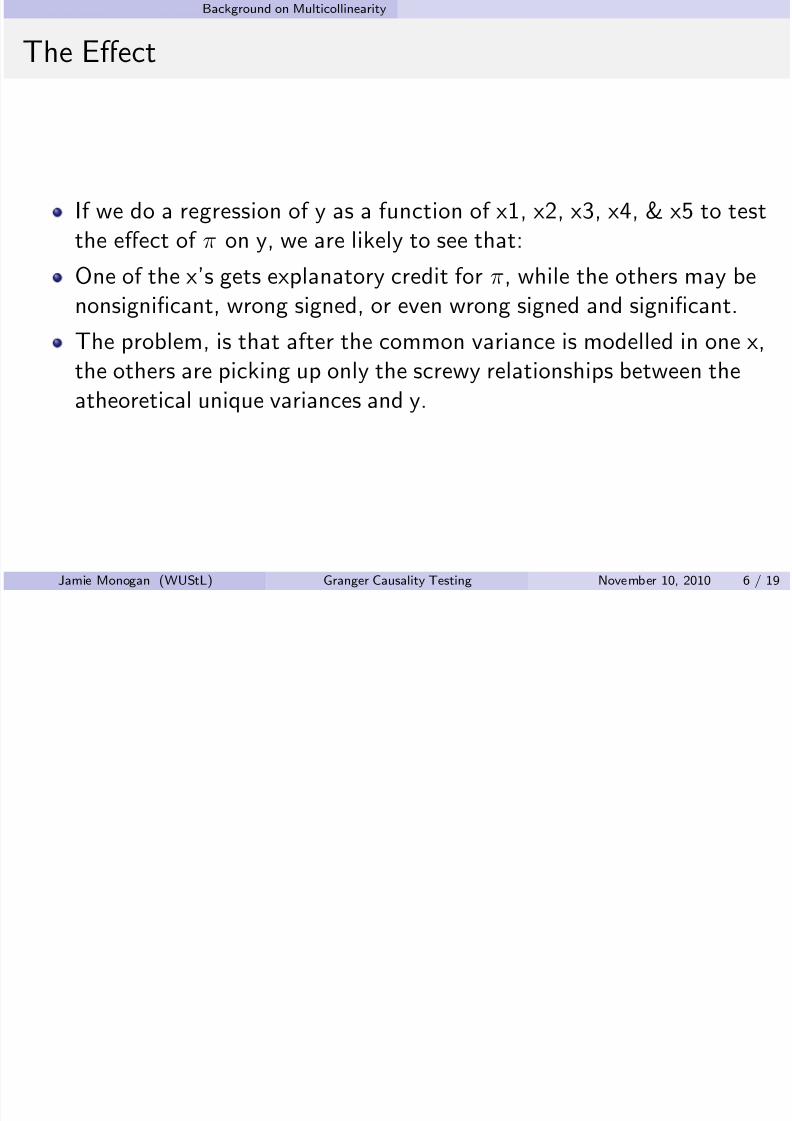
In this instance it is quite wrong to assert (blindly) that one of the x’sinfluences y and the others do not. If they tap the same concept,then you can’t know which of them represents π and which represents

meaningless unique variances.

The correct approach is not to try to separate effects at all if they areinseparable and to ask the theoretically correct question about π →y,not the individual x’s.

How? Block exclusion (F) test.



8/6/2019 13granger



Nested Model Test (Dropping q Parameters)

Produce R2’s for an unrestricted model (UR) and a restricted version(R) that drops several parameters.

Then a test of the restriction is:

F q ,N −k = (R 2UR − R 2R )/q (1 − R 2UR )/(N − k )

Where q is the number of dropped parameters, N is the number of observatons, and k is the number of parameters in the unrestricted

model.Note: For the special case of 1 parameter, F=t2 for that parameterand p (F)= p (t) and thus we do not need a block exclusion test.



8/6/2019 13granger



Software

R

Run the restricted and unrestricted models as separate “lm” objects(perhaps “model.ur” and “model.r”).

Then, “anova(model.ur, model.r)” will offer the F -test on therestrictions.

Stata

In Stata, simply estimate the unrestricted model and then ask for anF -test on several variables in the model

It will still yield a comparison of R2

with and without particularcoefficient restrictions.

To test the exclusion of d, e, and f:1 reg y a b c d e f 2 test d e f



8/6/2019 13granger



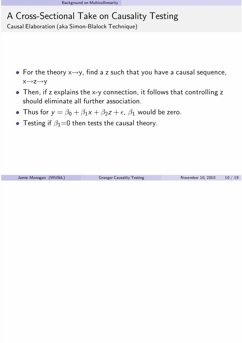
A Cross-Sectional Take on Causality TestingCausal Elaboration (aka Simon-Blalock Technique)

For the theory x→y, find a z such that you have a causal sequence,x→z→y

Then, if z explains the x-y connection, it follows that controlling zshould eliminate all further association.

Thus for y = β 0 + β 1x + β 2z + , β 1 would be zero.

Testing if β 1

=0 then tests the causal theory.


The Direct Granger Test

8/6/2019 13granger


g

The “Attitude” of the Granger Test

We are often in the position of having about equally good theoriesand research programs that posit both x→y and y→x.

So we specify our model according to theory and get contrary results.

Researchers on both sides, according to Granger—and later moreemphatically Sims—are arrogant about theory and data.

And since they get contrary results, at least one of them is wrong.

So we turn to causality testing in humility, admitting that we do not

know the right model and just asking the data to speak to us.



8/6/2019 13granger


g

A Substantive Example: The Macro Polity Model

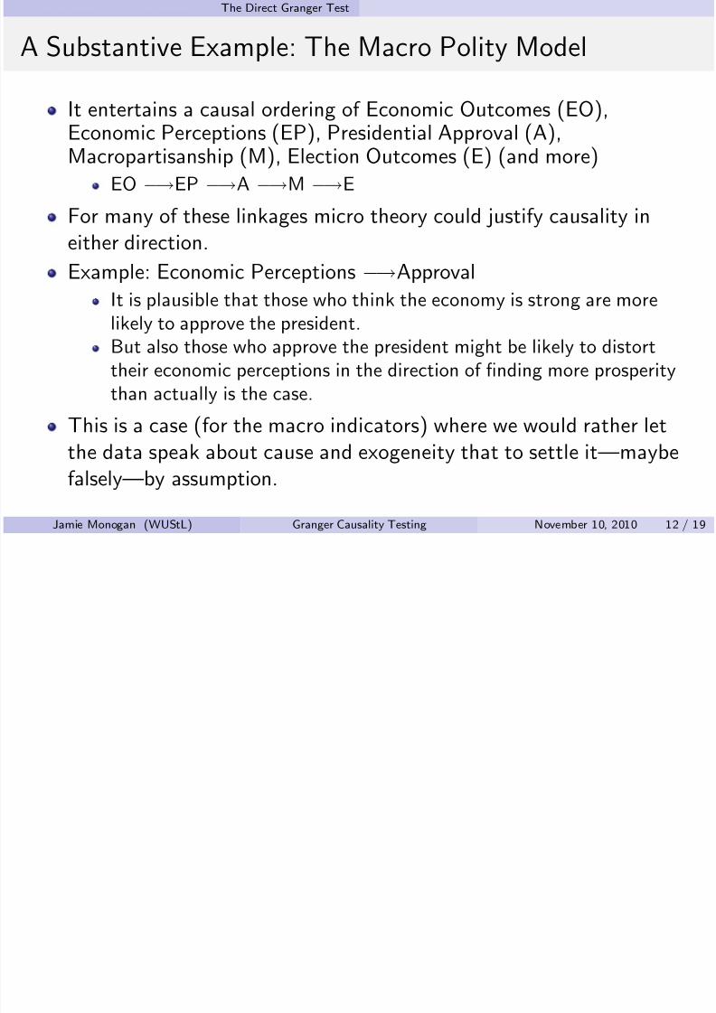
It entertains a causal ordering of Economic Outcomes (EO),

Economic Perceptions (EP), Presidential Approval (A),Macropartisanship (M), Election Outcomes (E) (and more)

EO −→EP −→A −→M −→E

For many of these linkages micro theory could justify causality in

either direction.Example: Economic Perceptions −→Approval

It is plausible that those who think the economy is strong are morelikely to approve the president.But also those who approve the president might be likely to distort

their economic perceptions in the direction of finding more prosperitythan actually is the case.

This is a case (for the macro indicators) where we would rather letthe data speak about cause and exogeneity that to settle it—maybefalsely—by assumption.



8/6/2019 13granger


g

Granger Causality

Intuition: if x→y then perturbing x (∆x) leads to later changes in y(∆y)

Asymmetry: if x→y then perturbing y (∆y) has no effect on futurevalues of x

Definition: A series x may be said to cause a series y if and only if theexpectation of y given the history of x is different from theunconditional expectation of Y.

E(y| y t −k , x t −k ) = E (y | y t −k )



8/6/2019 13granger



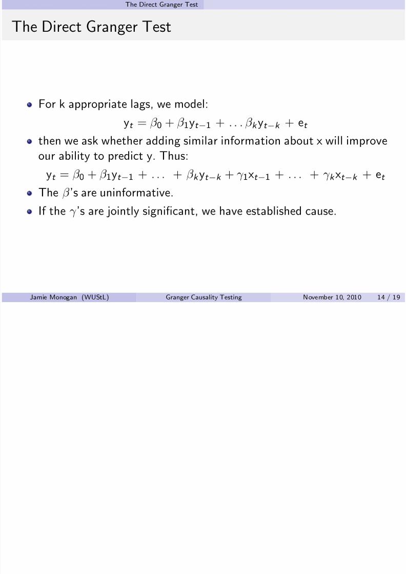
For k appropriate lags, we model:

yt = β 0 + β 1yt −1 + . . . β k yt −k + et

then we ask whether adding similar information about x will improveour ability to predict y. Thus:

yt = β 0 + β 1yt −1 + . . . + β k yt −k + γ 1xt −1 + . . . + γ k xt −k + et

The β ’s are uninformative.

If the γ ’s are jointly significant, we have established cause.



8/6/2019 13granger


Exogenity: The Mirror Image

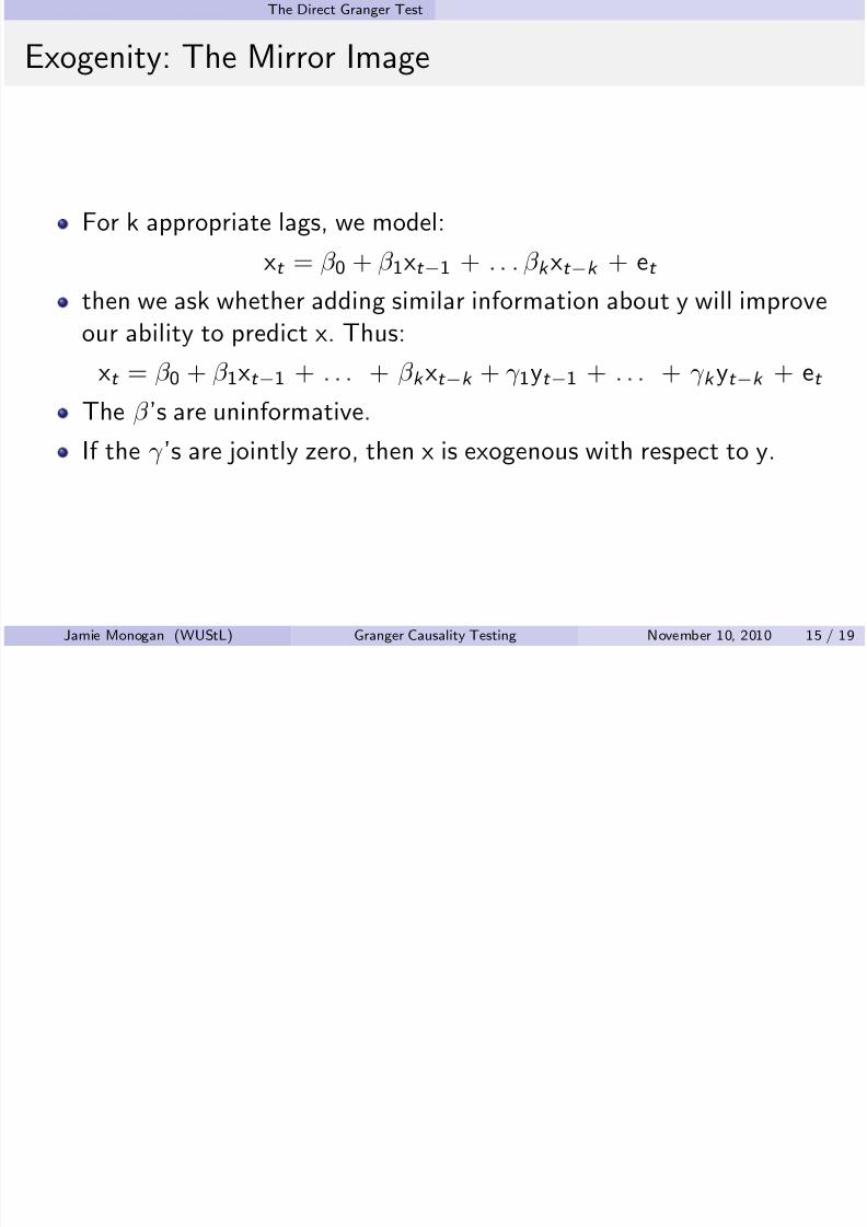
For k appropriate lags, we model:

xt = β 0 + β 1xt −1 + . . . β k xt −k + et

then we ask whether adding similar information about y will improveour ability to predict x. Thus:

xt = β 0 + β 1xt −1 + . . . + β k xt −k + γ 1yt −1 + . . . + γ k yt −k + et

The β ’s are uninformative.

If the γ ’s are jointly zero, then x is exogenous with respect to y.



8/6/2019 13granger


Software

R

Create a “tsunion” data set with several lags of y & xRun two “lm” objects with y as the DV: one with lagged x’s(y.with.x) and one without (y.without.x)

anova(y.with.x, y.without.x), significant F implies x→y

Then the reverse: Run two “lm” objects with x as the DV: one withlagged y’s (x.with.y) and one without (x.without.y)

anova(x.with.y, x.without.y), nonsignificant F implies yx

Stata

reg y l(1/4).y l(1/4).x

test l(1/4).x, significant F implies x→y

Then the reverse: reg x l(1/4).x l(1/4).y

test l(1/4).y, nonsignificant F implies y

xJamie Monogan (WUStL) Granger Causality Testing November 10, 2010 16 / 19


8/6/2019 13granger


Direct Granger vs. Box-Jenkins Prewhitening

See Freeman (1983).

Both approaches are similar in that they first control for expectedpatterns of autodependence in the dependent variable, and then claim

causation when the cleaned series are associated with the independentvariable.

The difference is that Box-Jenkins modeling uses an empiricaltechnique to identify the best simple model of autodependencewhereas Granger modeling is more brute force, including serveral lags

of y so that dependence may be modeled out even without knowingexactly what it is.



8/6/2019 13granger


Theoretical Issues

The Direct Granger test violates the correct specification assumptionof OLS, since the correct specification is assumed to be unknown.

It relies on overfitting to make sure that all the autodependence

process is removed from the data.Overfitting is harmless as regards unbiasedness, but causes estimatorinefficiency.

Consequently the Granger coefficients are not optimal and should not

be used. That is, the direct Granger test should be used as asignificance test only, not as a source of structural coefficients.



8/6/2019 13granger


For next time:

Read Enders 5.5-5.9 and Brandt & Williams chapter 2.

Download HWarmsRace.csv (remember: “read.csv”)Use a direct Granger test to show if there is a causal relationshipbetween the defense expenditures of India and Pakistan. If there is,are the expenditures of one country exogenous to the other’s?


Documents

13granger