Embed Size (px)
Citation preview
arX
iv:1
004.
2354
v1 [
cs.O
H]
14
Apr
201
0
Kinematic modelling of a 3-axis NC machine tool in linear and circular
interpolation
The International Journal of Advanced Manufacturing Technology
Xavier Pessoles, Yann Landon and Walter Rubio
Universite de Toulouse; INSA, UPS, Mines Albi, ISAE; ICA (Institut Clement Ader);
135, avenue de Rangueil, F-31077 Toulouse, France
Tel.: +33-(0)5-61558176
Abstract
Machining time is a major performance criterion when it comes to high speed machining. CAM soft-
ware can help in estimating that time for a given strategy. But in practice, CAM programmed feed rates
are rarely achieved, especially where complex surface finishing is concerned. This means that machining
time forecasts are often more than one step removed from reality. The reason behind this is that CAM
routines do not take either the dynamic performances of the machines or their specific machining toler-
ances into account. The present article seeks to improve simulation of high speed NC machine dynamic
behaviour and machining time prediction, offering two models. The first contributes through enhanced
simulation of 3-axis paths in linear and circular interpolation, taking high speed machine accelerations
and jerks into account. The second model allows transition passages between blocks to be integrated in
the simulation by adding in a polynomial transition path that caters for the true machining environment
tolerances. Models are based on respect for path monitoring. Experimental validation shows the con-
tribution of polynomial modelling of the transition passage due to the absence of a leap in acceleration.
Simulation error on the machining time prediction remains below 1%.
Keywords
High speed machining; Linear interpolation; Circular interpolation; Polynomial transition
1
Nomenclature
Kinematic and dynamic parameters−→J jerk vector−→A acceleration vector−→V feed rate vector−→X position vector
Jmax,i maximum jerk limited by machine
dynamics on the axis i
Amax,i maximum acceleration limited by the
machine dynamics on the axis i
A0,i, V0,i,
X0,i
acceleration, feed rate and initial po-
sition on the axis i
VF programmed feed rate
V ′F feed rate reached if VF is not
achieved
Vc,i feed rate set on the axis i
VIn feed rate of entry into a block
VOut feed rate exiting a block
V ′Out feed rate exiting a block if VOut is not
reached
Vdisc maximum feed rate for entering a dis-
continuity
Vj feed rate entering a discontinuity lim-
ited by jerk
Va feed rate entering a discontinuity lim-
ited by acceleration
τi duration of phase i (τi = Ti − Ti−1)
2
Circular transitions in linear interpolation
A,O,B theoretical programmed path
A,Q,B path described by the machine
TIT , tolx,
toly
method to define point Q in accor-
dance with the programming method
R radius of the arc inserted on transi-
tion
l1, l2 length covered before and after the
transition
β angle formed by segments [AO] and
[OB]
ac, jt normal acceleration and tangential
jerk in steady state
Circular transitions in circular interpolation
R1, R2 radii of circles before and after a cir-
cle - circle transition
Parameters used in circular interpolation
O centre of circle
R radius of circle
P (t) current point
α angle covered by the circle arc
θ(t) current angle
Ji curvilinear jerk limited by the axis i
JC curvilinear jerk
Ai curvilinear acceleration limited by
the axis i
AC curvilinear acceleration
3
Polynomial transitions in linear interpolation
R frame(
O,−→X,
−→Y ,
−→Z)
A,O,B programmed theoretical path
(xA, yA, zA) coordinates of−→OA in the frame R
(xB, yB, zB) coordinates of−−→OB in the frame R
M point of entry into the discontinuity
N point of exit from the discontinuity
Q effective point of passage in the dis-
continuity
T time of passage in the discontinuity
L distance OM
P (t) current point
φi, θi spherical coordinates of the point i
tolx, toly, tolztolerance of position on the axes
VM , VN feed rates for entry on M and exit on
N
1 Introduction
High speed machining centres allow for extremely high feed rates to be programmed. However, when
machining molds or dies, dynamic performances of the machines do not always allow such feed rates to be
reached. Indeed, according to the quality sought, the segments making up the machining path are often
extremely short and in such conditions the feed rate reached by the machine will then be limited by the
NC interpolation time or even the capabilities in jerk or acceleration of the axes [1], [2]. The feed rate
will then not be constant, leading to considerably lower productivity, a variation in tangential cutting
forces and impaired quality [3]. Many publications relating to the search to reduce the number of feed
rate changes base their research on the use of NURBS interpolations. [4] [5] [6] or B-spline [7]. However,
in the industrial world, linear and circular interpolation remain the most frequently used methods on
many workpieces. Precise simulation of this type of movement is therefore essential.
The aim of this work is therefore to propose a comprehensive model intended to simulate the posi-
tion, feed rate, acceleration and jerk in 3-axis linear and circular interpolation taking the machine/NC
combination parameters into account.
At present, NC machine manufacturers [8] propose a displacement law on the axes in trapezoid
acceleration. This type of command has been studied in the literature by a number of authors writing on
uniaxial paths with null initial and final feed rates [9] [10]. This movement involves 7 phases (figure 1):
4
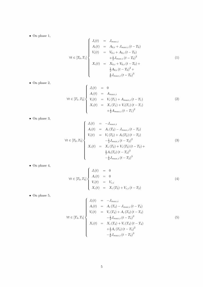
• On phase 1,
∀t ∈ [T0, T1]
Ji(t) = Jmax,i
Ai(t) = A0,i + Jmax,i (t− T0)
Vi(t) = V0,i +A0,i (t− T0)
+ 12Jmax,i (t− T0)
2
Xi(t) = X0,i + V0,i (t− T0) +
12A0,i (t− T0)
2 +
16Jmax,i (t− T0)
3
(1)
• On phase 2,
∀t ∈ [T1, T2]
Ji(t) = 0
Ai(t) = Amax,i
Vi(t) = Vi (T1) +Amax,i (t− T1)
Xi(t) = Xi (T1) + Vi(T1) (t− T1)
+ 12Amax,i (t− T1)
2
(2)
• On phase 3,
∀t ∈ [T2, T3]
Ji(t) = −Jmax,i
Ai(t) = Ai (T2)− Jmax,i (t− T2)
Vi(t) = Vi (T2) +Ai(T2) (t− T2)
− 12Jmax,i (t− T2)
2
Xi(t) = Xi (T2) + Vi (T2) (t− T2)+
12Ai(T2) (t− T2)
2
− 16Jmax,i (t− T2)
3
(3)
• On phase 4,
∀t ∈ [T3, T4]
Ji(t) = 0
Ai(t) = 0
Vi(t) = Vc,i
Xi(t) = Xi (T3) + Vc,i (t− T3)
(4)
• On phase 5,
∀t ∈ [T4, T5]
Ji(t) = −Jmax,i
Ai(t) = Ai (T4)− Jmax,i (t− T4)
Vi(t) = Vi (T4) +Ai (T4) (t− T4)
− 12Jmax,i (t− T4)
2
Xi(t) = Xi (T4) + Vi (T4) (t− T4)
+ 12Ai (T4) (t− T4)
2
− 16Jmax,i (t− T4)
3
(5)
5
• On phase 6,
∀t ∈ [T5, T6]
Ji(t) = 0
Ai(t) = −Amax,i
Vi(t) = Vi (T5)−Amax,i (t− T5)
Xi(t) = Xi (T5) + Vi(T5) (t− T5)
− 12Amax,i (t− T5)
2
(6)
• On phase 7,
∀t ∈ [T6, T7]
Ji(t) = Jmax,i
Ai(t) = Ai (T6) + Jmax,i (t− T6)
Vi(t) = Vi (T6) +Ai (T6) (t− T6)
+ 12Jmax,i (t− T6)
2
Xi(t) = Xi (T6) + Vi (T6) (t− T6)
+ 12Ai (T6) (t− T6)
2
+ 16Jmax,i (t− T6)
3
(7)
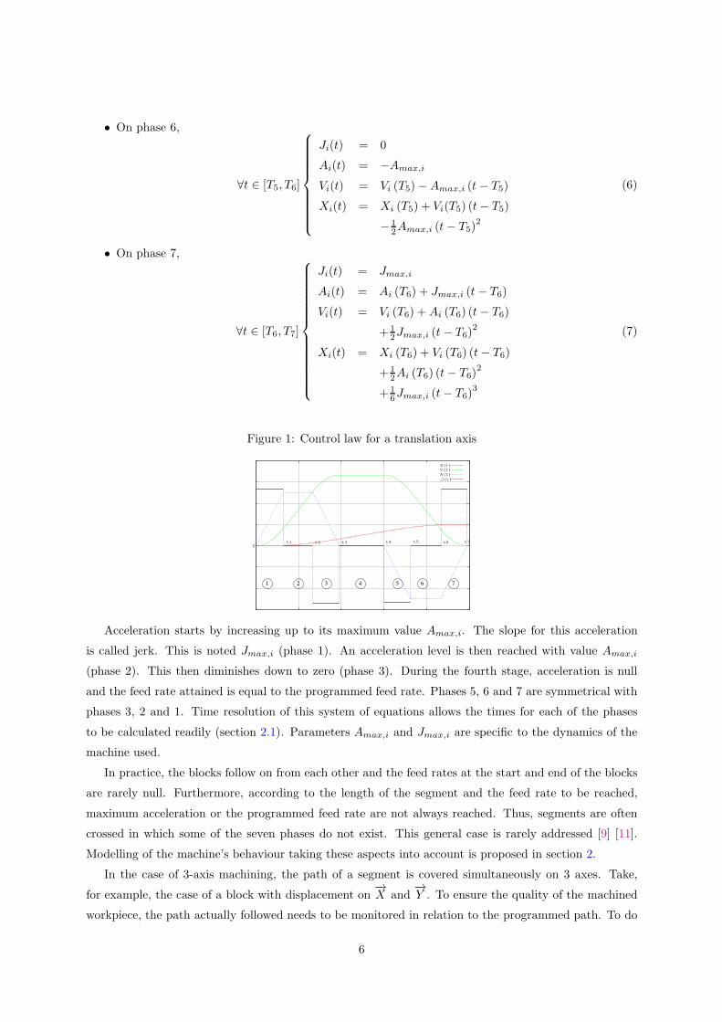
Figure 1: Control law for a translation axis
0
X(t)V(t)A(t)
J(t)
2 4 61 753
t1 t2 t3 t4 t5 t6 t7
Acceleration starts by increasing up to its maximum value Amax,i. The slope for this acceleration
is called jerk. This is noted Jmax,i (phase 1). An acceleration level is then reached with value Amax,i
(phase 2). This then diminishes down to zero (phase 3). During the fourth stage, acceleration is null
and the feed rate attained is equal to the programmed feed rate. Phases 5, 6 and 7 are symmetrical with
phases 3, 2 and 1. Time resolution of this system of equations allows the times for each of the phases
to be calculated readily (section 2.1). Parameters Amax,i and Jmax,i are specific to the dynamics of the
machine used.
In practice, the blocks follow on from each other and the feed rates at the start and end of the blocks
are rarely null. Furthermore, according to the length of the segment and the feed rate to be reached,
maximum acceleration or the programmed feed rate are not always reached. Thus, segments are often
crossed in which some of the seven phases do not exist. This general case is rarely addressed [9] [11].
Modelling of the machine’s behaviour taking these aspects into account is proposed in section 2.
In the case of 3-axis machining, the path of a segment is covered simultaneously on 3 axes. Take,
for example, the case of a block with displacement on−→X and
−→Y . To ensure the quality of the machined
workpiece, the path actually followed needs to be monitored in relation to the programmed path. To do
6
so, synchronization of the axes is needed. Indeed, both axes must reach the final position at the same
instant. Thus, on 3 axes, a feed rate, an acceleration and a maximum jerk have to be calculated for each
of the axes as a function of the slowest axis [12]. Using the model in 7 phases, the same time for each of
the phases will be obtained on each of the axes, allowing the path to be followed.
Circular interpolation is also widely used. However, as far as can be ascertained, there are no publica-
tions covering changes in feed rate on a circle while also ensuring monitoring of the path to be followed.
Modelling of such a case will be presented in section 2.
Moreover, a machining operation can be broken down into a multitude of linear or circular blocks.
This thus poses the problem of the crossing of transitions between discontinuous blocks tangent to each
other. From a purely kinematic point of view, the exact passage by the programmed points requires
precise arrest of the machine at the end of each block. This behaviour is not permitted in practice as
it implies repeatedly slowing down and thus a loss in productivity. In addition, the jerks are prejudicial
to the quality of the workpieces manufactured as well as the lifetime of the cutting tools used. Thus, in
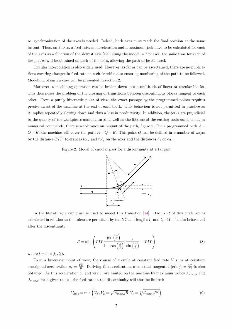
numerical commands, there is a tolerance on pursuit of the path, figure 2. For a programmed path A –
O – B, the machine will cover the path A – Q – B. This point Q can be defined in a number of ways:
by the distance TIT , tolerances tolx and toly on the axes and the distances d1 or d2.
Figure 2: Model of circular pass for a discontinuity at a tangent
In the literature, a circle arc is used to model this transition [14]. Radius R of this circle arc is
calculated in relation to the tolerance permitted by the NC and lengths l1 and l2 of the blocks before and
after the discontinuity:
R = min
TITcos(
β2
)
1− cos(
β2
) ,l
sin(
β2
) − TIT
(8)
where l = min (l1, l2).
From a kinematic point of view, the course of a circle at constant feed rate V runs at constant
centripetal acceleration ac =V 2
F
R . Deriving this acceleration, a constant tangential jerk jt = V 3
R2 is also
obtained. As this acceleration ac and jerk jt are limited on the machine by maximum values Amax,i and
Jmax,i, for a given radius, the feed rate in the discontinuity will thus be limited:
Vdisc = min
(
VF , Va =√
Amax,iR, Vj =3
√
Jmax,iR2
)
(9)
7
This modelling allows the maximum speed of passage to be expressed as a discontinuity. However, it
pre-supposes a jump in acceleration: at constant feed rate on segment [AO] acceleration is null (phase 4)
while at constant speed on a circle, the projection of the acceleration vector on the axes can reach V 2F /R.
This leap in acceleration on crossing the transition is not observed in practice. Thus, a circular model
cannot be used to simulate precisely the position, feed rate, acceleration and jerk along the discontinuity,
even if it gives a good approximation of the drop in feed rate. In part 3, a polynomial form of modelling
for transitions between non-tangent segments will be presented.
In circular interpolation, the transitions between the circles of different radii need to be modelled. In
this case, the same type of limitation arises: two tangent circles with different radii are discontinuous in
curvature. On crossing the discontinuity, there will thus be a jump in acceleration. Pateloup [15] proposes
a model to determine the minimum feed rate needed to cross the discontinuity taking into account the
jerk j, the radii R1 and R2 of the two circular portions, and the interpolation time δt of the machine:
Vdisc =
√
R1R2
|R1 −R2| δtj(10)
This model is also used to cross a transition between a segment of a straight line and a circle arc when
they are tangent. The model is again taken up in the algorithm proposed by Tapie [1] to calculate the
entry rate into this type of discontinuity. This method for crossing discontinuities will be validated in
section 4.
With the aim of simulating a complete path (path including blocks and transitions), Lavernhe [12]
proposes a method allowing the machine’s dynamic behaviour to be computed using a formalism with
inverse time. Integration of the NC cycle time in this method allows it to predict the control jerk value
to be predicted for each of the periods. From this are deduced the plots for acceleration and feed rate.
Furthermore, his model takes the predictive functions available on NCs into account. The model for
crossing of discontinuities in tangency is that described previously (circle arc).
Another solution is to identify the servo-system model for the machine/NC combination [13]. This
approach appears difficult to implement given the lack of data provided by NC manufacturers. Indeed,
to apply this approach would require precise knowledge of the slaving flow diagrams for the axes and
especially the various correctors used. Where appropriate, tests need to be conducted to identify the
transfer function parameters.
Finally, a third method involves modelling directly the laws described in the previous sections. The
difficulty in implementing these models lies in calculating for each block the time for each acceleration
phase as well as the jerk on each axis. Integration of anticipation is no easy matter.
To sum up, the paths of linear blocks are clearly described in the literature. However, the general case
(path of a segment at non-null initial and final feed rates) is not studied. Furthermore, no information is to
be found on the path of circular blocks. With respect to discontinuities in tangency, the model for passage
in a circle arc allows the feed rate on crossing the discontinuity to be quantified but does not enable laws
for feed rates and accelerations to be modelled. The idea is to propose algorithms that, on 3 axes, show
how to go from a feed rate on block entry VIn to a feed rate on block exit VOut while attempting to reach
the programmed rate VF both in linear interpolation (section 2.1) and circular interpolation (section 2.3).
8
A model is then proposed for passage into discontinuities in tangency between two straight lines (section
3). Finally, tests validating the simulator are presented.
2 Modelling NC behaviour in linear and circular interpolation
In this section, the laws for displacements, feed rates, accelerations and jerks to cover a uniaxial
segment from a feed rate VIn to a feed rate VOut passing through a feed rate VF are modelled. Passage
in the case of a 3-axis segment is then studied. The results are then adapted to circular interpolation.
2.1 Modelling uniaxial linear segments in the general case
In the general case of a toolpath for a segment in 3-axis machining, the feed rates at entry, middle
and exit of a segment will not be identical. In addition, according to the jumps in feed rate to be crossed
and the length of the displacement to be made, the feed rate will not necessarily be reached. As a result,
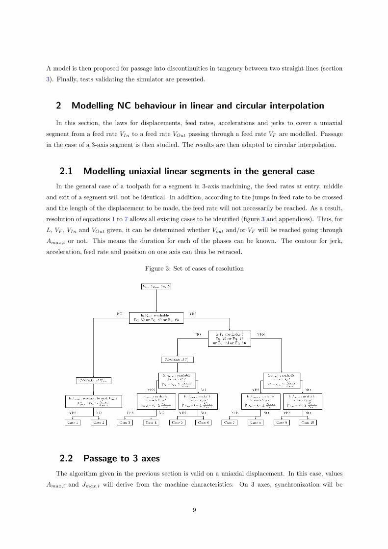
resolution of equations 1 to 7 allows all existing cases to be identified (figure 3 and appendices). Thus, for
L, VF , VIn and VOut given, it can be determined whether Vout and/or VF will be reached going through
Amax,i or not. This means the duration for each of the phases can be known. The contour for jerk,
acceleration, feed rate and position on one axis can thus be retraced.
Figure 3: Set of cases of resolution
2.2 Passage to 3 axes
The algorithm given in the previous section is valid on a uniaxial displacement. In this case, values
Amax,i and Jmax,i will derive from the machine characteristics. On 3 axes, synchronization will be
9
needed. This means that the times for each of the 7 phases are identical on all axes. As a result, for a
given displacement at a given programmed feed rate, the NC will recalculate a set feed rate, acceleration
and jerk for each of the axes.
The modelling method followed is thus as follows: for a given segment, the displacement to be made
on each of the axes is calculated. Using the results of the previous section with maximum acceleration
and maximum jerk, it will thus be possible to determine which of the 3 axes will be the slowest. Then,
using the results Lavernhe offers [12], feed rates Vi, accelerations Ai and jerks Ji on the axes limited i
can thus be calculated as a function of the distance Llim to be covered on the limiting axis and distances
Li to be covered on the limited axes:
Vi =Li
LlimVF Ai =
Li
LlimAmax,i Ji =
Li
LlimJmax,i (11)
All the elements used to simulate tool paths in 3-axis linear interpolation have thus been presented. In
what follows, the case of circular interpolation will be studied.
2.3 Modelling tool paths defined by circle arcs
As has been seen, few data are given as to simulation of displacements on a circle. The problem
involves understanding how the axes of the NC behave to follow a circular path and especially how
decelerations and accelerations are made when following a circle. To this purpose, the laws governing a
circular movement can be stated.
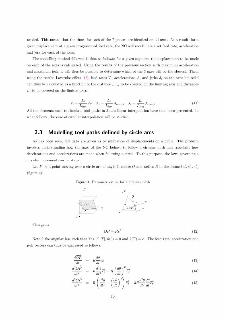
Let P be a point moving over a circle arc of angle θ, centre O and radius R in the frame (−→er ,−→eα,−→ez)(figure 4).
Figure 4: Parametrization for a circular path
This gives:−−→OP = R−→er (12)
Note θ the angular law such that ∀t ∈ [0, T ], θ(0) = 0 and θ(T ) = α. The feed rate, acceleration and
jerk vectors can thus be expressed as follows:
d−−→OP
dt= R
dθ
dt−→eθ (13)
d2−−→OP
dt2= R
d2θ
dt2−→eθ −R
(
dθ
dt
)2−→er (14)
d3−−→OP
dt3= R
(
d3θ
dt3−(
dθ
dt
)3)
−→eθ − 3Rd2θ
dt2dθ
dt−→er (15)
10
When the set feed rate is reached, dθ(t)/dt = VF /R. Nevertheless, the angle law θ(t) is unknown on
passage from null feed rate to the programmed feed rate. As a result, using a law in 7 phases is proposed,
like that considered in section 2.1. In these conditions the jerk effect no longer corresponds to a jerk by
axis, but a “curvilinear” jerk taking into account the influence of 2 or 3 axes along the plane in which
the circle is made. This jerk is thus the result of several contributing axes. This means the tool path has
to be expressed as a projection on the machine’s axes of translation. This is done through two moves in
frames.
Let M1 and M2 be the respective matrices for passage of the frame (−→u ,−→v ,−→w ) towards frame
(−→x ,−→y ,−→z ) and the frame (−→eR,−→eθ ,−→ez) towards frame (−→u ,−→v ,−→w ).
M is noted as the matrix for passage of the frame (−→x ,−→y ,−→z ) to frame (−→eR,−→eθ ,−→ez):
M = (M1M2)−1
(16)
2.4 Calculation of jerk and curvilinear acceleration
Curvilinear jerk and curvilinear acceleration do not form part of the machine parameters, but they
are the result of the contribution made by accelerations and jerks for each axis in movement. According
to the zone in which the circle is completed, one or other of the axes will be limiting.
These parameters are calculated at the start and the end of movement as that is where they are most
significant. Indeed, for the path of a circle arc, one needs to switch from a null normal acceleration to
a normal acceleration equivalent to V 2F /R at the start and at the end of the path, which would require
an infinite jerk at the start or the end of the path. As this can only be considered on certain types of
machining centres, the maximum jerk that can be reached at the start and end of the path in consideration
of the characteristics of the axes is thus calculated.
Consider a circle arc made in the frame (−→u ,−→v ,−→w ) from an angle θ(0) = 0 to an angle θ(T ) = α, T
being the overall duration of the path. In this general case, the matrix M is a matrix for rotation of
the orthonormed frame (−→eR,−→eθ ,−→ez) to the orthonormed frame (−→x ,−→y ,−→z ). This matrix is thus orthogonal
and can be inverted. Note (ux, uy, uz), (vx, vy, vz), (wx, wy, wz) the coordinates of the vectors −→u , −→v , −→win the frame (−→x ,−→y ,−→z ).
Using a model in 7 phases for angular acceleration and assuming initial acceleration to be null, the
following is obtained on the first phase, ∀t ∈ [0, T1]:
d3θdt3 (t) = Jcd2θdt2 (t) = Jct
dθdt (t) = θIn + 1
2Jct2
θ(t) = θInt+16Jct
3
(17)
with Jc the curvilinear jerk. Carrying over equation 17 into equation 15 on t = 0 and projecting onto
the machine axes, the following is obtained:
11
d3−−→OP
dt3= R
(
Jc − θ3In
)−→eθ =
R(
Jc − θ3In
)
vx
R(
Jc − θ3In
)
vx
R(
Jc − θ3In
)
vx
(−→x ,−→y ,−→z )
(18)
Jerk is limited on each of the axes and curvilinear jerk will depend on 2 or even 3 axes. The latter
will thus depend on the axis that will be limiting. The following will therefore obtain:
J1 =Jmax,x
Rvx+ θ3In J2 =
Jmax,y
Rvy+ θ3In J3 =
Jmax,z
Rvz+ θ3In (19)
Similarly, J4, J5, J6 are calculated at the end of movement to obtain:
Jc = mini∈[1,6]
(Ji) (20)
Curvilinear acceleration Ac can now be calculated. Noting θ1, the position reached at the end of phase
1 and θ1 the feed rate reached at the end of phase 1, the following will obtain in phase 2, ∀t ∈ [T1, T2]:
d3θdt3 (t) = 0
d2θdt2 (t) = Ac
dθdt (t) = θ1 +Act
θ(t) = θ1 + θ1t+12Act
2
(21)
Carrying over equation 21 into equation 14, this gives t = T1:
d2−−→OPdt2 = RAc
−→eθ −Rθ12−→er
=(
− (ux cos θ1 + vx sin θ1)Rθ21
+(uy cos θ1 + vy sin θ1)RAc
)
· −→x+(
− (−ux sin θ1 + vx cos θ1)Rθ21
+(−uy sin θ1 + vy cos θ1)RAc
)
· −→y+(
− wxRθ21 + wyRAc
)
· −→z
(22)
Thus:
A1 =Amax,x+(ux cos θ+vx sin θ)Rθ2
1
(uy cos θ+vy sin θ)R
A2 =Amax,y+(−ux sin θ1+vx cos θ1)Rθ2
1
(−uy sin θ1+vy cos θ1)R
A3 =Amax,z+wxRθ2
1
wyR
(23)
The same method is adopted for the deceleration phase, giving:
Ac = mini∈[1,6]
(Ai) (24)
To conclude, in the modelling proposed in circular interpolation, the angular law follows a movement
in seven phases, with maximum jerk being the calculated value Jc and maximum acceleration being the
calculated value Ac. Knowing all the parameters of a circle arc (point of departure, point of arrival,
radius, etc.), the machine’s dynamic behaviour can be simulated throughout the circular path.
12
This part allows the laws of position, feed rate, acceleration and jerk on unique blocks in circular
and linear interpolation to be simulated. What remains is to model the junctions between blocks. It has
already been shown that the model for transition between two tangent paths functions. The following
part of the article will cover how to model the passage between two linear segments.
3 Modelling of the transition between two rectilinear blocks
In the literature, transitions between two segments are always modelled by circle arcs, though this
does not seem to match the real behaviour of the machine. Knowing that NCs are capable of describing
polynomials of degree 5, it is suggested that they be used to model discontinuities in tangency. This
model should allow a criterion for feed rate for entry into the discontinuity to be defined as also the
contour for position, feed rate, acceleration and jerk in the discontinuity.
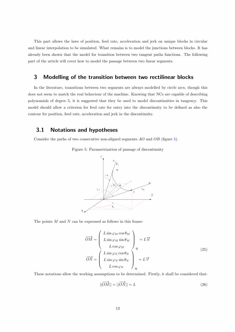
3.1 Notations and hypotheses
Consider the paths of two consecutive non-aligned segments AO and OB (figure 5).
Figure 5: Parametrization of passage of discontinuity
The points M and N can be expressed as follows in this frame:
−−→OM =
L sinϕM cos θM
L sinϕM sin θM
L cosϕM
R
= L−→u
−−→ON =
L sinϕN cos θN
L sinϕN sin θN
L cosϕN
R
= L−→v
(25)
These notations allow the working assumptions to be determined. Firstly, it shall be considered that:
||−−→OM || = ||−−→ON || = L (26)
13
Then, considering the problem to be symmetrical, this gives:
−−→OQ = ||−−→OQ|| ·
−→u +−→v||−→u +−→v || = ||−−→OQ|| · −→w =
Qx
Qy
Qz
R
(27)
The coordinates of point Q can then be expressed in the frame R:
−−→OQ = ||−−→OQ|| ·
sinϕQ cos θQ
sinϕQ sin θQ
cosϕQ
R
ϕQ = arccos wz√w2
x+w2y+w2
z
Si wx ≥ 0 , θQ = arcsinwy√
w2x+w2
y
Si wx < 0 , θQ = π − arcsinwy√
w2x+w2
y
(28)
The direction of the vector−−→OQ is thus fully determined by the vectors −→u and −→v . Its norm now needs
to be determined. This is done by the tolerance granted the machine on passage of the discontinuity
(section 1 and figure 1). In this instance, tolx, toly and tolz denote the maximum tolerances for passage
used by the NC on each of the axes−→X ,
−→Y and
−→Z , which means that:
−−→OQ · −→X ≤ tolx−−→OQ · −→Y ≤ toly−−→OQ · −→Z ≤ tolz
(29)
The norm of vector−−→OQ can thus be calculated as follows:
||−−→OQ|| = min
(
tolx| sinϕQ cos θQ|
,toly
| sinϕQ sin θQ|,
tolz| cosϕQ|
,
)
(30)
Finally, due to the problem’s symmetry, it can be considered that the entry feed rate in the disconti-
nuity ||−→VM || and the exit feed rate ||−→VN || will be equal:
−→VM = −VIn
−→u −→VN = VIn
−→v (31)
As points A, M and O, as well as points B, N and O are aligned, angles ϕM , θM , ϕN and θN can
thus be calculated:
ϕM = arccos zA√x2
A+y2
A+z2
A
Si xA ≥ 0 , θM = arcsin yA√x2
A+y2
A
Si xA < 0 , θM = π − arcsin yA√x2
A+y2
A
ϕN = arccos zB√x2
B+y2
B+z2
B
Si xB ≥ 0 , θN = arcsin yB√x2
B+y2
B
Si xB < 0 , θN = π − arcsin yB√x2
B+y2
B
(32)
14
3.2 Formation of the equation
Using a polynomial representation, the equation for the position, feed rate, acceleration and jerk of
the point P in the discontinuity thus takes the following form, ∀t ∈ [0, T ]:
−−→OP (t) =
∑5i=0 ait
i
∑5i=0 bit
i
∑5i=0 cit
i
(33)
d−−→OP (t)
dt=
∑5i=1 iait
i−1
∑5i=1 ibit
i−1
∑5i=1 icit
i−1
(34)
d2−−→OP (t)
dt2=
∑5i=2
i!(i−2)!ait
i−2
∑5i=2
i!(i−2)!bit
i−2
∑5i=2
i!(i−2)!cit
i−2
(35)
d3−−→OP (t)
dt2=
∑5i=3
i!(i−3)!ait
i−3
∑5i=3
i!(i−3)!bit
i−3
∑5i=3
i!(i−3)!cit
i−3
(36)
3.3 Boundary conditions
In order to resolve this system, eight boundary conditions are used:
−−→OP (0) =
−−→OM (37)
−−→OP (T ) =
−−→ON (38)
−−→OP
(
T
2
)
=−−→OQ (39)
−→V (0) =
−→VM = −VIn
−→u (40)
−→V (T ) =
−→VN = VIn
−→v (41)
−→A (0) =
−→0 (42)
−→A (T ) =
−→0 (43)
−→J
(
T
2
)
=−→0 (44)
Equations 37 and 38 translate entry into the discontinuity. Equation 39 translates the problem’s
symmetry, meaning that the point parametrized by tolerances of passage is reached half way through the
time of the path. Considering that acceleration is null at entry and exit of the discontinuity, equations
42 and 43 are obtained. To conclude, equation 44 translates symmetry of the acceleration contour.
15
3.4 Resolution
This thus involves resolving a system of 24 scalar equations (projection of equations 37 onto 44) whose
unknowns are:
• 18 coefficients ai, bi, ci of polynomials,
• the norm L of vectors−−→OM and
−−→ON ,
• time T for passage of the transition.
Resolving the system gives:
a0 = 16Qx sinϕM cos θM3(sinϕN cos θN+sinϕM cos θM )
b0 =16Qy sinϕM sin θM
3(sinϕN sin θN+sinϕM sin θM)
c0 = 16Qz cosϕM
3(cosϕN+cosϕM )
(45)
a1 = −VIn sinϕM cos θM
b1 = −VIn sinϕM sin θM
c1 = −VIn cosϕM
(46)
a2 = 0
b2 = 0
c2 = 0
(47)
a3 =9(sinϕN cos θN+sinϕM cos θM)3V 3
In
1024Q2x
b3 =9(sinϕN sin θN+sinϕM sin θM )3V 3
In
1024Q2y
c3 =9(cosϕN+cosϕM )3V 3
In
1024Q2z
(48)
a4 = − 27(sinϕN cos θN+sinϕM cos θM)4V 4
In
65536Q3x
b4 = − 27(sinϕN sin θN+sinϕM sin θM )4V 4
In
65536Q3y
c4 = − 27(cosϕN+cosϕM )4V 4
In
65536Q3z
(49)
a5 = 0
b5 = 0
c5 = 0
(50)
−−→OP (T ) =
−−→ON ⇐⇒
T
T
T
=
32Qx
3VIn(sinϕN cos θN+sinϕM cos θM)32Qy
3VIn(sinϕN sin θN+sinϕM sin θM)
32Qz
3VIn(cosϕN+cosϕM )
(51)
−−→OP
(
T2
)
=−−→OQ ⇐⇒
L
L
L
=
16Qx
3(sinϕN cos θN+sinϕM cos θM )16Qy
3(sinϕN sin θN+sinϕM sin θM )
16Qz
3(cosϕN+cosϕM)
(52)
16
Due to the relation between Qx, Qy and Qz, the 3 expressions allowing L or T to be computed give
the same results. With respect to the feed rate on entry of the discontinuity VIn, it is ex ante equal to
the feed rate at the end of the upstream block. Nevertheless, it can perhaps be limited by maximum jerk,
maximum acceleration and the length of the blocks upstream and downstream from the transition. This
feed rate can now be calculated.
3.5 Feed rate on entry in the discontinuity
Expressing the problem as an equation allows the entry feed rate to be calculated when it is limited
by acceleration or maximum jerk: the assumption is made that maximum jerk is at point M and that
acceleration will be at its maximum at Q. Care must therefore be taken to ensure that the machine’s
capabilities are not exceeded at these points.
If the maximum jerk is reached on each of the axes, the equation gives:
−→J (0) =
−−−−→Jmax,i ⇐⇒ 6
a3
b3
c3
=
Jmax,x
Jmax,y
Jmax,z
(53)
According to the case, resolution of this system allows the entry rate limited by an axial jerk to be
determined using the results given by equation 48:
Vlim,j = 83|sinϕN cos θN+sinϕM cos θM | ·min
(
3
√
Q2xJmax,x, 3
√
Q2yJmax,y, 3
√
Q2zJmax,z
) (54)
Similarly, it is known that on the discontinuity, acceleration is at its maximum on T/2. The entry
feed rates that will be limited by acceleration can then be determined by resolving the following equation:
−→A
(
T
2
)
=−−−−→Amax,i (55)
By inserting this condition into equation 35 and using the results given by equations 48 and 49, the
following is obtained:
Vlim,a = 83|sinϕN cos θN+sinϕM cos θM | min
(
√
QxAmax,x,√
QyAmax,y,√
QzAmax,z
) (56)
Thus, maximum acceleration on each of the axes also leads to limitations on the feed rate on entering
the block:
VIn = min (VF , Vlim,j , Vlim,a) (57)
Finally, a last case remains: the transition length calculated L can be greater than the length of
the segment upstream or downstream. An additional condition is thus imposed: if L > ||−→OA||/2 or
L > ||−−→OB||/2, the coordinates of point Q are recalculated taking L = min(
||−→OA||/2, ||−−→OB||/2)
from
equation 52. Equations 54 and 56 then allow the limit feed rate on entry in the discontinuity to be
recalculated.
The proposed model is now complete. Experimental validation is proposed in the following section.
17
4 Experimental validation
Measurements of position profiles, feed rates and acceleration were made on a machine with the aim
of validating modelling. Tests were conducted on a DMU 50 eVo 5-axis machining centre equipped with
a Siemens 840D Numerical Control. The characteristics of the NC and machine combination are given in
table 1. This NC allows measurements of position, feed rate and acceleration to be made for a maximum
period of 10 seconds.
Table 1: Characteristics DMU 50 eVo - Siemens 840 D
Dynamic characteristics of axes
Maximum feed rate Vmax,i = 50 m/min
Maximum acceleration Amax,i = 9, 8 m/s2
Maximum jerk in translation Jmax,i = 40 m/s3
Maximum jerk on passage of Jcmax = 60 m/s3
a discontinuity in curvature
Characteristics of the NC
Tolerances on the axes Tol = 0, 01 mm
Interpolation time of NC 2ms
A test campaign enabled the proposed models to be validated. In particular, feed rates ranging from
500 to 10000mm/min and machining tolerances from 0.1 to 0.01mm on various paths were tested. More-
over, as the NC allowed certain dynamic parameters to be modified, jerk was also subjected to variation.
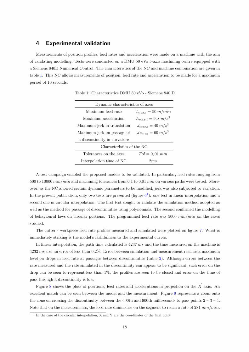
In the present publication, only two tests are presented (figure 61): one test in linear interpolation and a
second one in circular interpolation. The first test sought to validate the simulation method adopted as
well as the method for passage of discontinuities using polynomials. The second confirmed the modelling
of behavioural laws on circular portions. The programmed feed rate was 5000 mm/min on the cases
studied.
The cutter - workpiece feed rate profiles measured and simulated were plotted on figure 7. What is
immediately striking is the model’s faithfulness to the experimental curves.
In linear interpolation, the path time calculated is 4237 ms and the time measured on the machine is
4232 ms i.e. an error of less than 0.2%. Error between simulation and measurement reaches a maximum
level on drops in feed rate at passages between discontinuities (table 2). Although errors between the
rate measured and the rate simulated in the discontinuity can appear to be significant, such error on the
drop can be seen to represent less than 1%, the profiles are seen to be closed and error on the time of
pass through a discontinuity is low.
Figure 8 shows the plots of positions, feed rates and accelerations in projection on the−→X axis. An
excellent match can be seen between the model and the measurement. Figure 9 represents a zoom onto
the zone on crossing the discontinuity between the 600th and 900th milliseconds to pass points 2 – 3 – 4.
Note that on the measurements, the feed rate diminishes on the segment to reach a rate of 281 mm/min.
1In the case of the circular interpolation, X and Y are the coordinates of the final point
18
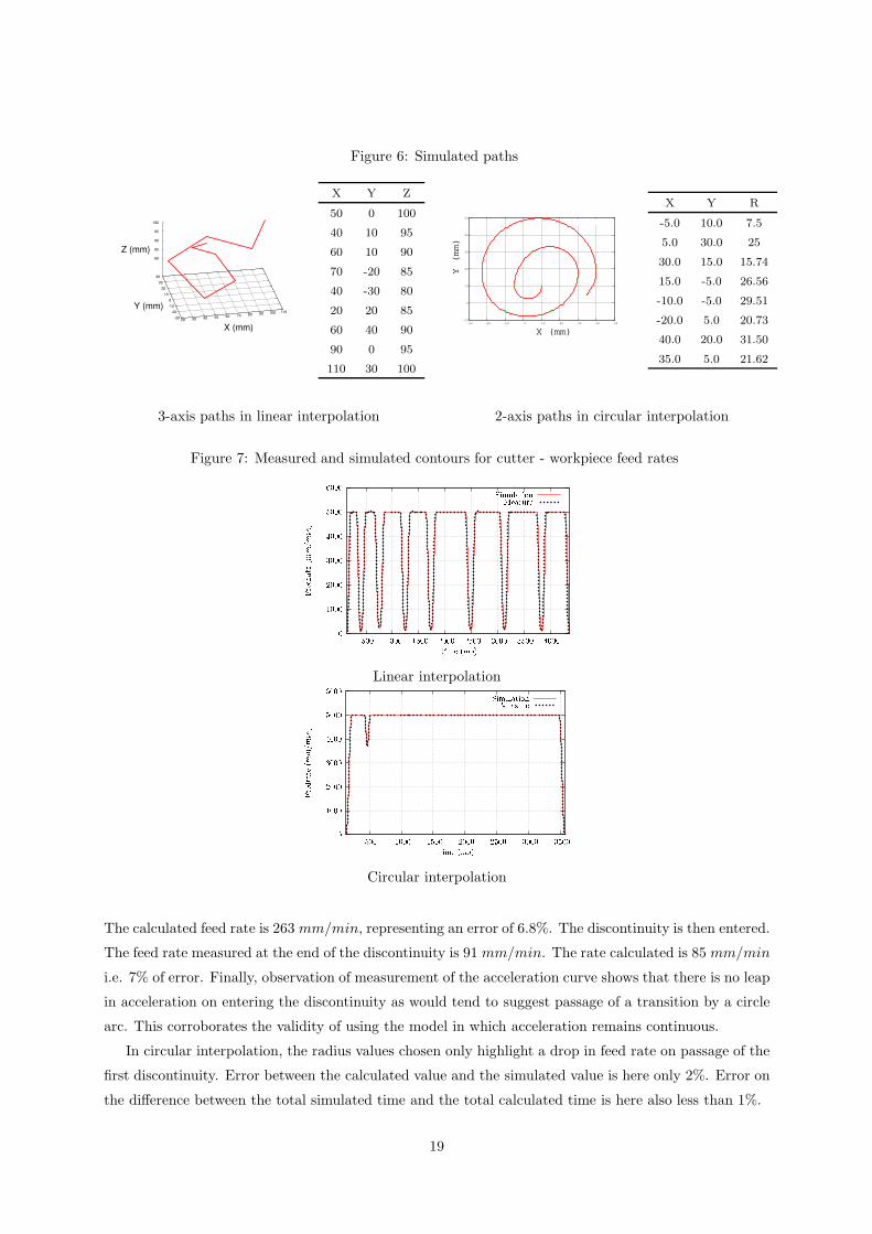
Figure 6: Simulated paths
20 30 40 50 60 70 80 90 100 110
-30
-20
-10
0
10
20
30
40
80
85
90
95
100
Z (mm)
Y (mm)
X (mm)
X Y Z
50 0 100
40 10 95
60 10 90
70 -20 85
40 -30 80
20 20 85
60 40 90
90 0 95
110 30 100
-10
0
10
20
30
40
50
-30 -20 -10 0 10 20 30 40 50
Y (mm)
X (mm)
X Y R
-5.0 10.0 7.5
5.0 30.0 25
30.0 15.0 15.74
15.0 -5.0 26.56
-10.0 -5.0 29.51
-20.0 5.0 20.73
40.0 20.0 31.50
35.0 5.0 21.62
3-axis paths in linear interpolation 2-axis paths in circular interpolation
Figure 7: Measured and simulated contours for cutter - workpiece feed rates
Linear interpolation
Circular interpolation
The calculated feed rate is 263 mm/min, representing an error of 6.8%. The discontinuity is then entered.
The feed rate measured at the end of the discontinuity is 91 mm/min. The rate calculated is 85 mm/min
i.e. 7% of error. Finally, observation of measurement of the acceleration curve shows that there is no leap
in acceleration on entering the discontinuity as would tend to suggest passage of a transition by a circle
arc. This corroborates the validity of using the model in which acceleration remains continuous.
In circular interpolation, the radius values chosen only highlight a drop in feed rate on passage of the
first discontinuity. Error between the calculated value and the simulated value is here only 2%. Error on
the difference between the total simulated time and the total calculated time is here also less than 1%.
19
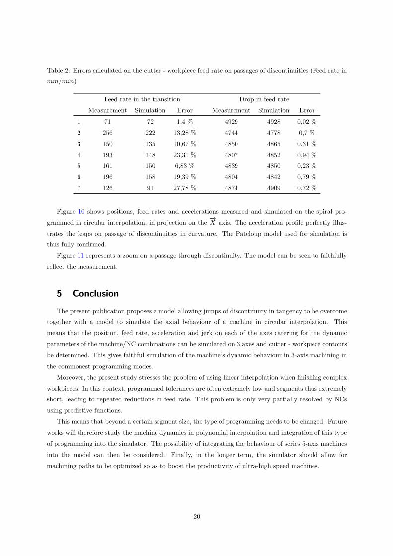
Table 2: Errors calculated on the cutter - workpiece feed rate on passages of discontinuities (Feed rate in
mm/min)
Feed rate in the transition Drop in feed rate
Measurement Simulation Error Measurement Simulation Error
1 71 72 1,4 % 4929 4928 0,02 %
2 256 222 13,28 % 4744 4778 0,7 %
3 150 135 10,67 % 4850 4865 0,31 %
4 193 148 23,31 % 4807 4852 0,94 %
5 161 150 6,83 % 4839 4850 0,23 %
6 196 158 19,39 % 4804 4842 0,79 %
7 126 91 27,78 % 4874 4909 0,72 %
Figure 10 shows positions, feed rates and accelerations measured and simulated on the spiral pro-
grammed in circular interpolation, in projection on the−→X axis. The acceleration profile perfectly illus-
trates the leaps on passage of discontinuities in curvature. The Pateloup model used for simulation is
thus fully confirmed.
Figure 11 represents a zoom on a passage through discontinuity. The model can be seen to faithfully
reflect the measurement.
5 Conclusion
The present publication proposes a model allowing jumps of discontinuity in tangency to be overcome
together with a model to simulate the axial behaviour of a machine in circular interpolation. This
means that the position, feed rate, acceleration and jerk on each of the axes catering for the dynamic
parameters of the machine/NC combinations can be simulated on 3 axes and cutter - workpiece contours
be determined. This gives faithful simulation of the machine’s dynamic behaviour in 3-axis machining in
the commonest programming modes.
Moreover, the present study stresses the problem of using linear interpolation when finishing complex
workpieces. In this context, programmed tolerances are often extremely low and segments thus extremely
short, leading to repeated reductions in feed rate. This problem is only very partially resolved by NCs
using predictive functions.
This means that beyond a certain segment size, the type of programming needs to be changed. Future
works will therefore study the machine dynamics in polynomial interpolation and integration of this type
of programming into the simulator. The possibility of integrating the behaviour of series 5-axis machines
into the model can then be considered. Finally, in the longer term, the simulator should allow for
machining paths to be optimized so as to boost the productivity of ultra-high speed machines.
20
Figure 8: Comparison of contours measured and simulated on a rectilinear path
Position
Feed rate
Acceleration
Acknowledgements
This work was carried out within the context of the working group Manufacturing 21 which brings
together 11 French research laboratories. The topics addressed are as follows:
• modelling of the manufacturing process,
• virtual machining,
• emerging manufacturing methods.
21
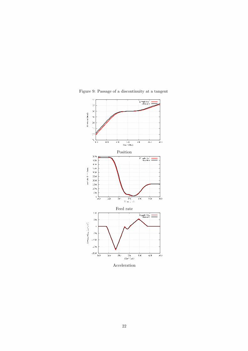
Figure 9: Passage of a discontinuity at a tangent
Position
Feed rate
Acceleration
22
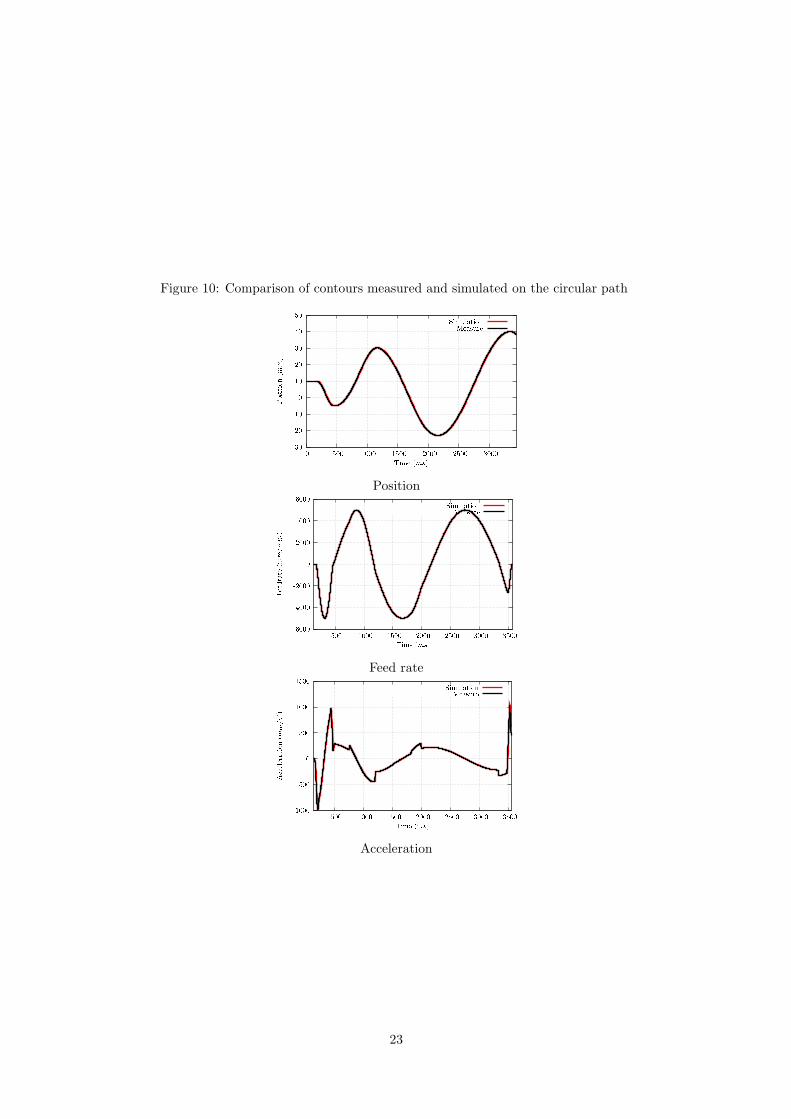
Figure 10: Comparison of contours measured and simulated on the circular path
Position
Feed rate
Acceleration
23
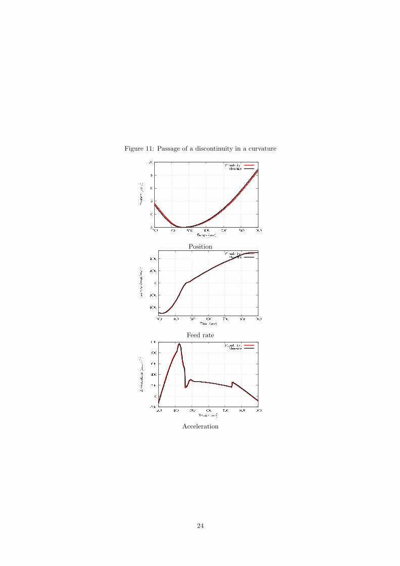
Figure 11: Passage of a discontinuity in a curvature
Position
Feed rate
Acceleration
24
References
[1] Tapie, L., Mawussi, K. & Anselmetti, B., Circular tests for HSM machine tools: Bore machining
application, International Journal of Machine Tools and Manufacture , 47(5), 805-819 (2007).
[2] Flores, V., Ortega, C., Alberti, M., Rodriguez, C A, de Ciurana, J. & Elias, A., Evaluation and
modeling of productivity and dynamic capability in high-speed machining centers, The International
Journal of Advanced Manufacturing Technology, 33(3), 403-411 (2007).
[3] Korkut, I. & Donertas, M., The influence of feed rate and cutting speed on the cutting forces, surface
roughness and tool-chip contact length during face milling, Materials & Design , 28(1), 308-312 (2007).
[4] Tsai, M.-., Cheng, C.-. & Cheng, M.-., A real-time NURBS surface interpolator for precision three-axis
CNC machining, International Journal of Machine Tools and Manufacture , 43(12), 1217-1227 (2003).
[5] Liu, X. et al., Adaptive interpolation scheme for NURBS curves with the integration of machining
dynamics, International Journal of Machine Tools and Manufacture , 45(4-5), 433-444 (2005).
[6] Xu, R. Z., Xie,L. , Li, C. X., & Du, D. S., Adaptive parametric interpolation scheme with limited
acceleration and jerk values for NC machining, The International Journal of Advanced Manufacturing
Technology , 36(3), 343-354 (2008).
[7] Sencer, B. & Altintas, Y., Feed optimization for five-axis CNC machine tools with drive constraints,
International Journal of Machine Tools and Manufacture , 48(7-8), 733-745 (2008).
[8] Siemens, http://www.automation.siemens.com/doconweb.
[9] Erkorkmaz, K. & Altintas, Y., High speed CNC system design. Part I: jerk limited trajectory genera-
tion and quintic spline interpolation, International Journal of Machine Tools and Manufacture, 41(9),
1323-1345 (2001).
[10] Aguilar, I. H., Commande des bras manipulateurs et retour visuel pour des applications a la robotique
de service, PhD Thesis, Universite de Toulouse III (2006).
[11] Nam, S. & Yang, M., A study on a generalized parametric interpolator with real-time jerk-limited
acceleration, Computer-Aided Design , 36(1), 27-36 (2004).
[12] Lavernhe, S., Tournier, C. & Lartigue, C., Kinematical performance prediction in multi-axis machin-
ing for process planning optimization. The International Journal of Advanced Manufacturing Technol-
ogy , 37(5), 534-544 (2008).
[13] Tounsi, N., Bailey, T. & Elbestawi, M.A., Identification of acceleration deceleration profile of feed
drive systems in CNC machines, International Journal of Machine Tools and Manufacture , 43(5),
441-451 (2003).
[14] Manuel & A, C., Influence of tool path strategy on the cycle time of high-speed milling, Computer-
Aided Design , 35(4), 395-401 (2003).
25
[15] Pateloup, V., Duc, E. & Ray, P., Corner optimization for pocket machining, International Journal
of Machine Tools and Manufacture, 44(12-13), 1343-1353 (2004).
Appendices: General case for the path of a uniaxial segment
The non-linear system described in section 1 therefore needs to be resolved. This resolution involves
resolving the 10 cases shown in figure 3.
The assumption is made that acceleration is null on entry and exit of the block. This is verified when
the segments are long enough to reach the feed rate programmed at the end of the segment (section 3.5).
Resolution of this system means the times for each of the phases can be determined so as to plot the
cutter - workpiece feed rate profile. In some cases, the programmed feed rate will not be reached and the
rate actually reached will be sought.
According to the distance to be covered and the jumps in feed rate to be crossed, 10 cases were listed.
From resolution of equations 1 to 7, the following obtains:
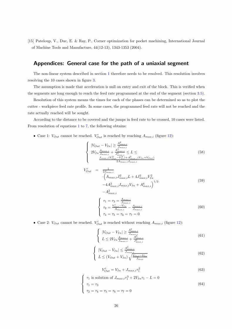
• Case 1: VOut cannot be reached. V ′Out is reached by reaching Amax,i (figure 12):
|VOut − VIn| ≥ A2
max,i
Jmax,i
2VInAmax,i
Jmax,i+
A3
max,i
J2
max,i
≤ L ≤Jmax,i(V
2
Out−V 2
In)+A2
max,i(VIn+VOut)
2Amax,iJmax,i
(58)
V ′Out = 1
2Jmax,i
·(
Amax,iJ2max,iL+ 4J2
max,iV2In
−4A2max,iJmax,iVIn +A4
max,i
)1/2
−A2max,i
(59)
τ1 = τ3 =Amax,i
Jmax,i
τ2 =V ′
Out−VIn
Amax,i− Amax,i
Jmax,i
τ4 = τ5 = τ6 = τ7 = 0
(60)
• Case 2: VOut cannot be reached. V ′Out is reached without reaching Amax,i (figure 12):
|VOut − VIn| ≥A2
max,i
Jmax,i
L ≤ 2VInAmax,i
Jmax,i+
A3
max,i
J2
max,i
(61)
|VOut − VIn| ≤ A2
max,i
Jmax,i
L ≤ (VOut + VIn)√
VOut−VIn
Jmax
(62)
V ′Out = VIn + Jmax,iτ
21 (63)
τ1 is solution of Jmax,iτ31 + 2VInτ1 − L = 0
τ1 = τ3
τ2 = τ4 = τ5 = τ6 = τ7 = 0
(64)
26
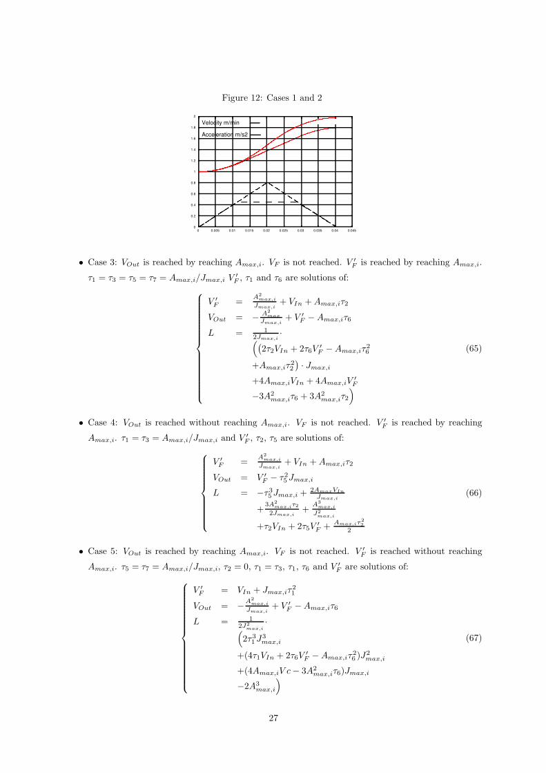
Figure 12: Cases 1 and 2
0
0.2
0.4
0.6
0.8
1
1.2
1.4
1.6
1.8
2
0 0.005 0.01 0.015 0.02 0.025 0.03 0.035 0.04 0.045
Velocity m/min
Acceleration m/s2
• Case 3: VOut is reached by reaching Amax,i. VF is not reached. V ′F is reached by reaching Amax,i.
τ1 = τ3 = τ5 = τ7 = Amax,i/Jmax,i V′F , τ1 and τ6 are solutions of:
V ′F =
A2
max,i
Jmax,i+ VIn +Amax,iτ2
VOut = − A2
max
Jmax,i+ V ′
F −Amax,iτ6
L = 12Jmax,i
·(
(
2τ2VIn + 2τ6V′F −Amax,iτ
26
+Amax,iτ22
)
· Jmax,i
+4Amax,iVIn + 4Amax,iV′F
−3A2max,iτ6 + 3A2
max,iτ2
)
(65)
• Case 4: VOut is reached without reaching Amax,i. VF is not reached. V ′F is reached by reaching
Amax,i. τ1 = τ3 = Amax,i/Jmax,i and V ′F , τ2, τ5 are solutions of:
V ′F =
A2
max,i
Jmax,i+ VIn +Amax,iτ2
VOut = V ′F − τ25 Jmax,i
L = −τ35 Jmax,i +2AmaxVIn
Jmax,i
+3A2
max,iτ22Jmax,i
+A3
max,i
J2
max,i
+τ2VIn + 2τ5V′F +
Amax,iτ2
2
2
(66)
• Case 5: VOut is reached by reaching Amax,i. VF is not reached. V ′F is reached without reaching
Amax,i. τ5 = τ7 = Amax,i/Jmax,i, τ2 = 0, τ1 = τ3, τ1, τ6 and V ′F are solutions of:
V ′F = VIn + Jmax,iτ
21
VOut = −A2
max,i
Jmax,i+ V ′
F −Amax,iτ6
L = 12J2
max,i
·(
2τ31J3max,i
+(4τ1VIn + 2τ6V′F −Amax,iτ
26 )J
2max,i
+(4Amax,iV c− 3A2max,iτ6)Jmax,i
−2A3max,i
)
(67)
27
• Case 6: VOut is reached without reaching Amax,i. VF is not reached. V ′F is reached without reaching
Amax,i. τ1 = τ3, τ5 = τ7, τ1, τ5 and V ′F are solutions of (figure 13) :
V ′F = τ31 Jmax,i + 2τ1VIn
VOut = V ′F − τ27 Jmax,i
L = −τ37 Jmax,i + τ31 Jmax,i + 2τ1VIn + 2τ7V′F
(68)
Figure 13: Case 6
-2
-1
0
1
2
3
4
5
6
0 0.02 0.04 0.06 0.08 0.1 0.12 0.14 0.16
Velocity (m/min)
Acceleration (m/s2)
• Case 7: VOut is reached by reaching Amax,i. VF is reached. VF is reached by reaching Amax,i.
|VF − VIn| ≥A2
max,i
Jmax,i
|VOut − VF | ≥A2
max,i
Jmax,i
L ≥ 12Amax,iJmax,i
·(
(
2Jmax,iVF + 2A2max,i
)
VIn
+Jmax,iV2F +A2
max,iVF
+(
2Jmax,iVOut + 2A2max,i
)
VF
+Jmax,iV2Out +A2
max,iVOut
)
(69)
τ1 = τ3 = τ5 = τ7 = Amax
Jmax
τ2 = VF
Amax− Amax
Jmax
τ6 = VOut
Amax− Amax
Jmax
(70)
• Case 8: VOut is reached without reaching Amax,i. VF is reached. VF is reached by reaching Amax,i.
|VF − VIn| ≥A2
max,i
Jmax,i
|VOut − VF | ≤ A2
max,i
Jmax,i
L ≥ (2Jmax,iVF+2A2
max,i)VIn+Jmax,iV2
F+A2
max,iVF
2Amax,iJmax,i
+√JmaxVOut(4VF+VOut)+AmaxVF
2Jmax
(71)
τ1 = τ3 =Amax,i
Jmax,i
τ2 = VF−VIn
Amax,i− Amax,i
Jmax,i
τ5 = τ7 =√
VF−VOut
Jmax,i
τ6 = 0
(72)
28
• Case 9: VOut is reached by reaching Amax,i. VF is reached. VF is reached without reaching Amax,i.
|VF − VIn| ≤ A2
max,i
Jmax,i
|VOut − VF | ≥ A2
max,i
Jmax,i
L ≥√JmaxVF (4VIn+VF )+AmaxVIn
2Jmax
+(2Jmax,iVOut+2A2
max,i)VF+Jmax,iV2
Out+A2
max,iVOut
2Amax,iJmax,i
(73)
τ1 = τ3 =√
VIn−VF
Jmax,i
τ2 = 0
τ5 = τ7 =Amax,i
Jmax,i
τ6 = VOut−VF
Amax,i− Amax,i
Jmax,i
(74)
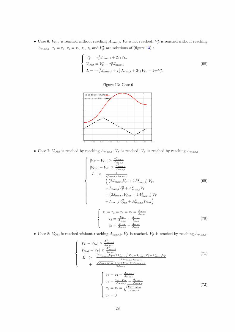
• Case 10: VOut is reached without reaching Amax,i. VF is reached. VF is reached without reaching
Amax,i (figure 14) :
|VF − VIn| ≤A2
max,i
Jmax,i
|VOut − VF | ≤A2
max,i
Jmax,i
L ≥√JmaxVF (4VIn+VF )+AmaxVIn
2Jmax
+√JmaxVOut(4VF+VOut)+AmaxVF
2Jmax
(75)
τ1 = τ3 =√
VIn−VF
Jmax,i
τ2 = 0
τ5 = τ7 =√
VF−VOut
Jmax,i
τ6 = 0
(76)
Figure 14: Case 10
-2
0
2
4
6
8
10
0 0.05 0.1 0.15 0.2 0.25 0.3
Velocity (m/min)
Acceleration (m/s2)
In the simulations, equation 2 is resolved by the Cardan method. The systems of equation 65, 66, 67
and 68 are non-linear. They are resolved numerically using the Newton-Raphson method.
To use this algorithm, take a segment of 0.01m to be covered. Take VIn = 0.2m/s, VOut = 0.1m/s,
VF = 0.5m/s. The machine parameters are those in table 1.
|VOut − VIn| ≤A2
max,i
Jmax,i; thus there will be no phase 2. L ≥ (VOut + VIn)
√
VOut−VIn
Jmax; the length of the
segment thus allows VOut to be reached.
29
|VF −VIn| ≤ A2
max,i
Jmax,iand |VOut−VF | ≤ A2
max,i
Jmax,iand L ≤
√JmaxVOut(4VF+VOut)+AmaxVF
2Jmax. The length does
therefore not allow VF to be reached and the differences in feed rates will not allow maximum acceleration
to be reached. This means case 6 applies. This givesV ′F = 0.4418m/s,
τ1 = τ3 = 0.07776s. τ5 = τ7 = 0.09245s.
30