1,2 Discussion started: 22 January 2018 c Author(s) … · Manuscript under review for journal Earth Syst. Sci. Data Discussion started: 22 January 2018 c. 4

1

Diversity II water quality parameters for 300 lakes worldwide from ENVISAT (2002-2012) Daniel Odermatt1,2, Olaf Danne2, Petra Philipson3, Carsten Brockmann2 1Odermatt & Brockmann GmbH, Zurich, 8005, Switzerland 2Brockmann Consult GmbH, Geesthacht, 20502, Germany 5 3Brockmann Geomatics Sweden AB, Kista, 164 40, Sweden

Correspondence to: Daniel Odermatt ([email protected])

1. Abstract.

The use of ground sampled water quality information for global studies is limited due to practical and financial constraints.

Remote sensing is a valuable means to overcome such limitations and to provide synoptic views of ambient water quality at 10

appropriate spatio-temporal scales. In past years several large data processing efforts were initiated to provide corresponding

data sources. The Diversity II water quality dataset consists of several monthly, yearly and 9-year averaged water quality

parameters for 340 lakes worldwide and is based on data from the full ENVISAT MERIS operation period (2002-2012).

Existing retrieval methods and datasets were selected after an extensive algorithm intercomparison exercise using in situ

reference measurements for more than 40 lakes representing a wide range of bio-optical conditions. Chlorophyll-a, total 15

suspended matter, turbidity, coloured dissolved organic matter, lake surface water temperature, cyanobacteria and floating

vegetation maps, as well as several auxiliary data layers, provide a generically specified data basis that can be used for

assessing a variety of locally relevant ecosystem properties and environmental problems. We demonstrate the use of the

products by illustrating and discussing remotely sensed evidence of lake-specific processes and prominent regime shifts

documented in literature. The Diversity II data are available from https://doi.pangaea.de/10.1594/PANGAEA.871462, and 20

Python scripts for their analysis and visualization are provided at https://github.com/odermatt/diversity/.

2. Introduction

Freshwater ecosystems have undergone more dramatic changes than any other type of ecosystems (Sectretariat of the

Convention on Biological Diversity, 2010). Lakes contain about 87% of all surface freshwater (Gleick, 1996). The major

threats that affect lakes and reservoirs are water level changes, toxic pollution, salinization, eutrophication, acidification, 25

sediment pollution and invasion of exotic species. Several upstream anthropogenic activities are related to these threats, such

as agriculture, forestry, grazing, mining, irrigation, urbanisation and dams, hydraulic engineering and industrial

development. All these pressures are interconnected and act concurrently to reduce water quality and contribute to the

deterioration of the ecosystem, including habitat loss and reduced biodiversity.

Earth Syst. Sci. Data Discuss., https://doi.org/10.5194/essd-2018-2

Ope

n A

cces

s Earth System

Science

DataD

iscussio

ns

Manuscript under review for journal Earth Syst. Sci. DataDiscussion started: 22 January 2018c© Author(s) 2018. CC BY 4.0 License.

2

The conditions of inland waters vary over a wide range of spatial and temporal scales, leading to important logistic and

economic difficulties to monitor them on a regular basis. Some countries have national or regional lake monitoring

programmes, which are primarily based on ground surveys. However ground surveys often fail to sample on appropriate

spatial and temporal scales. Other countries do not have monitoring programmes due to a lack of funds. The use of satellite

remote sensing is a potentially cost-effective and efficient way to supplement the conventional in-situ point sampling 5

surveys. Remotely sensed products for water availability and quality are complementary to in-situ data in terms of spatial

and temporal coverage. They provide synoptic views of spatial distribution unachievable by other means, and are ideally

suited to cover the broad range of space and time scales associated with inland water applications. However, remote sensing

is limited in terms of parameter coverage and depth resolution.

The Medium Resolution Imaging Spectrometer (MERIS) was operated by the European Space Agency (ESA) in 2002-2012 10

and demonstrated unparalleled capabilities for water quality remote sensing. Extensive reviews of popular retrieval methods

revealed a wide range of different algorithms, but the usage of MERIS data prevailed (Matthews, 2011; Odermatt et al.,

2012). The first globally representative lake water quality dataset from remote sensing provided a snapshot of chlorophyll-a

(CHL-a) concentrations in 80’000 lakes worldwide based on MERIS Full Resolution (FR) data acquired in 2011 (Sayers et

al., 2015). However, this dataset was compiled with an algorithm optimized for ocean colour remote sensing, whose 15

suitability for inland waters was disavowed on several occasions (see e.g. Mobley et al., 2004; Morel and Prieur, 1977).

Therefore we carried out an intercomparison of well-known and publicly available algorithms for the retrieval of CHL-a and

other water quality parameters in optically complex waters with a heterogeneous reference dataset for more than 40 lakes

(Odermatt et al., 2015a). The Diversity II water quality dataset is produced with the most suitable retrieval methods

identified through these investigations. 20

In addition to the optimized methodology, the Diversity II water quality dataset excels previous work by covering the full

MERIS operation period with monthly, yearly and 9-year product aggregates, and a several additional water quality

parameters. Hence it provides a generically specified data basis that can be used for assessing a variety of locally relevant

ecosystem properties and environmental problems. Several case studies are available that demonstrate such assessments with

lake-specific foci (Odermatt et al., 2015b), but the larger part of the dataset is yet to be exploited. 25

3. Input data

3.1. Geographical scope

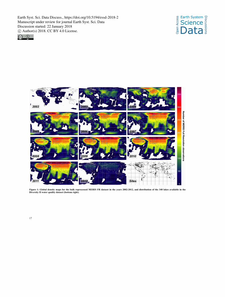
We selected 340 lakes for processing (Figure 1) based on their biodiversity relevance, size, auxiliary and reference data

availability, geographic distribution and particular user requests. 66 of those lakes are at least 50 km2 large and located

within Ramsar Wetlands or listed as LakeNet Biodiversity Priority sites (www.worldlakes.org). The data table 30

(https://doi.pangaea.de/10.1594/PANGAEA.871462?format=html#download) allows for their identification. The dataset

includes 250 of the world’s 350 largest lakes by extent, whereas size implies regional relevance and favours the feasibility of


Ope

n A

cces

s Earth System

Science

DataD

iscussio

ns


3

remote sensing retrievals in general and of Lake Surface Water Temperature (LSWT) in particular (Politi et al., 2016).

Various contributors provided in situ water quality measurements for 42 lakes, which are used as reference sites for quality

assessment (Odermatt et al., 2015a). The largest reservoirs in South America and individual sites in Asia and Australia are

included in order to improve the global representativeness. 50 additional lakes are included due to specific stakeholder

requests. 5

In principle, the Diversity II water quality dataset could be extended to a much larger number of lakes. Size is the most

important restriction in this regard, with a contiguous open water surface of roughly 1 km by 1 km being the theoretical

minimum, but certain complications occurring even for larger water bodies. The total number of suitable lakes worldwide is

expected to be between the 80’000 demonstrated by Sayers et al. (2015), and, neglecting shape properties, the 350’000 lakes

larger than 1 km2 identified by Verpoorter et al. (2014). 10

3.2. ENVISAT MERIS L1B FSG imagery

MERIS was operated in 2002-2012 on-board the near-polar orbiting ENVISAT satellite by the European Space Agency

(ESA; Rast et al., 1999). It measured reflected solar radiance in 15 narrow spectral bands across visible and near-infrared

(NIR) wavelengths. In FR mode, its push-broom charge-coupled device (CCD) arrays sampled the 1150 km wide swath at

approximately 260 by 290 m ground resolution in across track and along track direction, respectively. MERIS had a nominal 15

revisit time of 2-3 days at the equator and less at higher latitudes, but FR data was not systematically acquired in the early

years until 2005, and in later years it varied slightly due to mission operations, and therefore the availability of usable data

varies regionally and temporally (Figure 1).

We refer to three widely, but not consistently, used satellite image processing levels, in which Level 1 (L1) consists of Top-

Of-Atmosphere (TOA) signals, Level 2 (L2) includes derived geophysical quantities and Level 3 (L3) represents spatio-20

temporally aggregated data. Approximately 300’000 MERIS L1 images were used as input for the production of the

Diversity II water quality dataset. The data represents calibrated TOA radiance, also referred to as at-sensor radiance. It

emerged from the 2014 bulk reprocessing using MERIS Instrument Processing Facility version 6. Its geo-orthorectification

was improved using the Accurate MERIS Ortho-Rectified Geolocation Operational Software (AMORGOS; Bourg and

Etanchaud, 2007), thus the data is referred to as MERIS L1B Full-Swath Geo-corrected (FSG). 25

3.3. AATSR ARC-Lake LSWT products

The Diversity II water quality dataset includes Lake Surface Water Temperature (LSWT) products that were readily

provided by the ESA ARC-Lake project as version 3 production. The LSWT retrieval was performed with an optimal

estimation approach (MacCallum and Merchant, 2013, 2012). Lake-specific prior surface temperatures were generated using

an iterative scheme that is initiated with the monthly MODIS land and sea surface temperature climatologies. The ARC-Lake 30

processor then uses valid satellite observations, simulations with the FLake model (Mironov, 2008) and Data Interpolating


Ope

n A

cces

s Earth System

Science

DataD

iscussio

ns


4

Empirical Orthogonal Function (DINEOF; Alvera-Azcárate et al., 2005) techniques to iteratively create from this spatially

and inter-annually invariant initial guess a field of spatially resolved temperature fields.

Several product types using different processing techniques, spatial and temporal aggregations are available (MacCallum and

Merchant, 2014). We selected the DINEOF reconstructed, day- and night-time acquired monthly products in 0.05° spatial

resolution, whose file names are ALIDXXXX_PLREC9D_TS012SR.nc and ALIDXXXX_PLREC9N_TS012SR.nc, 5

respectively, with XXXX being a four-digit lake ID. They are available for 298 out of the 340 lakes considered, and an

empty LSWT product layers are contained in the remaining 42 lakes.

3.4. Auxiliary data

Each lake’s perimeter was defined in a shapefile that resulted from vectorized outlines of the Synthetic Aperture Radar

Water Bodies (SAR-WB) map created by Santoro and Wegmüller (2014). These perimeters represent the maximum extent 10

of water available from ENVISAT-ASAR acquisitions between 2002-2012, and each polygon’s area and circumference were

added to an attribute table. The polygons are intersected with the Global Lakes and Wetlands Database (GLWD; Lehner and

Döll, 2004) Level 1 dataset, and ambiguities were manually resolved. The merged tabulated attributes are available in a

metadata list (https://doi.pangaea.de/10.1594/PANGAEA.871462?format=html#download). Alternative lake names were

added to the list at every opportunity, but are neither exhaustive nor tracked. 15

Lake water surface level data (Crétaux et al., 2011) provided by the Laboratory of Studies on Spatial Geophysics and

Oceanography (LEGOS) through their Hydroweb portal (http://www.legos.obs-mip.fr/soa/hydrologie/hydroweb/) was

originally complementing and distributed with the Diversity II database. This data come as 1D discrete time samples, as

opposed to the 2D temporal aggregated water quality maps. Furthermore, it is based on independent developments and

updates that would require continuous mirroring. Due to these differences, we refrained from adding them to the Pangaea 20

Diversity II repository.

4. Data processing methods

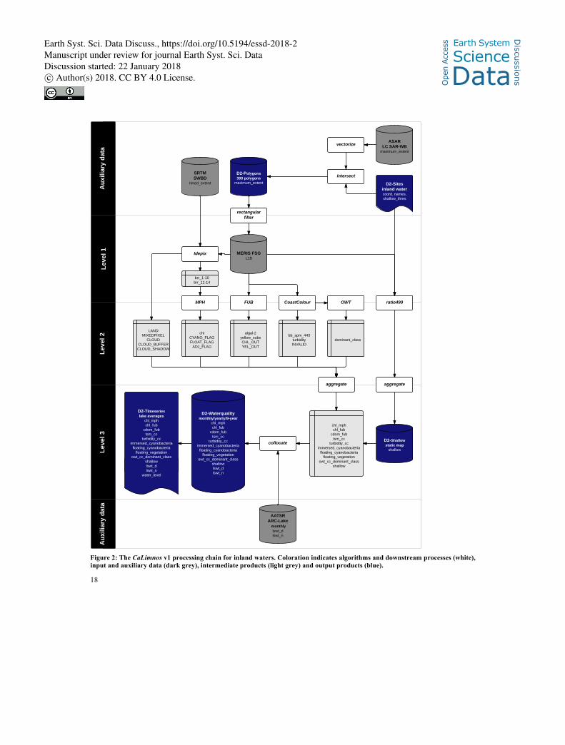
The bulk production of temporally aggregated water quality parameters from L1B and auxiliary data requires a combination

of several methods in an unsupervised processing chain. For this purpose we implemented the CaLimnos v1 processing chain

(Figure 2) for deployment on ESA’s Earth observation data processing cluster Calvalus (Fomferra et al., 2012). It is 25

composed of several processors for the ESA BEAM Toolbox (Fomferra and Brockmann, 2005), which has recently evolved

into the Sentinel Application Platform (SNAP). The same input and auxiliary data, pre- and post-processing modules were

also used to create 10-day aggregates for the investigation of phenological cycles in Lake Balaton (Palmer et al., 2015), and

corresponding CaLimnos v1 L2 intermediate outputs were used for assessing the spatio-temporal variability of CHL-a in

Lake Geneva (Kiefer et al., 2015). 30


Ope

n A

cces

s Earth System

Science

DataD

iscussio

ns


5

4.1. Pre-processing

The identification of pure water pixels is an essential pre-processing step, because even sub-pixel signal contributions from

land surfaces can strongly affect the retrieval procedures, especially when using band arithmetic algorithms that do not check

for input signal compliance at runtime. The Idepix algorithm is an open-source SNAP processor and performs such

identification for clouds, cloud shadows, cloud buffers, land, snow/ice, sun glint and mixed pixels (Danne, 2016) based on 5

bottom-of-Rayleigh reflectance (BRR; Santer et al., 1999). BRR is subject to a partial correction of atmospheric effects,

representing reflectance at the hypothetical boundary between an infinitesimally small aerosol layer and gaseous air layers

above. It is the preferred signal when background reflectance for the estimation of aerosol optical thickness is highly

uncertain, therefore BRR intermediate products are also used for the identification of shallow water areas and as input for the

Maximum Peak Height processor (Matthews et al., 2012) according to Figure 2. 10

Idepix uses the Shuttle Radar Topography Mission (SRTM) Water Body Dataset (SWBD; Slater et al., 2006) as a static a

priori land-water mask, which is a snapshot of global water surface extent between 56°S and 60°N in February 2000. It

applies several arithmetic expressions, a spectral unmixing algorithm for mixed pixel identification, and two back-

propagation Neural Networks (NN) for cloud identification to MERIS FSG L1B and BRR input data (Kirches et al., 2013).

Output is a pixel identification flag layer which is much better suited for water constituent retrieval than the original L1B 15

product flags (Ruescas et al., 2014). However, usage with inland waters is subject to two particular challenges. First, Idepix’

sea ice identification uses climatological auxiliary data that is not available for lakes, therefore lake ice identification is less

accurate. Second, ephemeral water surfaces that may extend far beyond the SRTM observed extent are always clipped to the

latter.

Bottom visibility is a critical and unmastered error source for water quality retrieval, because most algorithms that provide 20

concentrations of water constituents do not account for benthic reflectance contributions in these so-called optically shallow

waters. In fact, a pre-conditions for them is optically deep water (i.e. no bottom reflection). Sandy or vegetated substrates

cause surface-leaving signals that can closely resemble increased suspended sediment and phytoplankton concentrations in

the water column, respectively, and thus distort retrievals. Only very few algorithms are actually dealing with the detection

of optically deep water, and none of them applies to inland waters. Based on recommendations for clear coastal waters 25

(Cannizzaro and Carder, 2006) and own investigations, we defined a band ratio that evaluates the relative elevation of

oligotrophic lakes’ 555 nm water-leaving reflectance peak, but using BRR in three MERIS bands as input due to the lack of

robust automated atmospheric correction algorithms for such conditions (Eq. 1; Odermatt et al., 2015a).

IF ratio_ 490 = BRRband3 ⋅BRRband 7

(BRRband5 )2 < Thres, shallow = TRUE Eq. 1

Due to the ambiguity of certain substrates’ shallow water reflectance and deep-water reflectances, this optical signature alone 30

is prone to false positive identifications. It becomes much more robust when applied to temporally aggregated ratio_490 due

to the relative persistence of benthic features as opposed to the dynamically changing water composition. Summer half-year


Ope

n A

cces

s Earth System

Science

DataD

iscussio

ns


6

mean averages were selected after evaluation of several statistical aggregation methods. Corresponding aggregates are

composed of all cloud-free MERIS observations in May to October 2008 for the Northern hemisphere, and November 2008

to April 2009 for the Southern hemisphere. Lakes with constantly high turbidity, such as Lake Balaton, still trigger false

positives. Therefore each ratio_490 aggregate map was verified with high-resolution satellite imagery and bathymetry

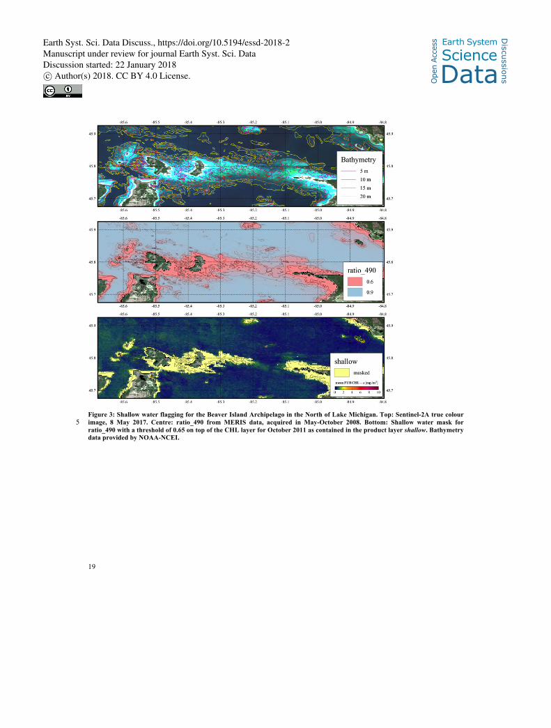
information. Considerable shallow water areas in about 30 oligo- to mesotrophic lakes were masked using a threshold of 5

0.65, which, in the case of the Beaver Island Archipelago in Lake Michigan, masks areas that are between 5-10 m deep

(Figure 3). Pixels removed in such manner are indicated in a separate product layer (shallow, Figure 3 bottom). In the Lake

Michigan example, there are some patterns in the chl_fub product that still resemble bathymetry features, but their

concentration levels are within variations for deep water areas apart from a few individual pixels. Especially in more turbid

lakes, lower thresholds are applied to prevent false positives according to the corresponding column in the lakes list 10

(https://doi.pangaea.de/10.1594/PANGAEA.871462?format=html#download).

4.2. Water quality retrieval

CHL-a retrieval in optically complex waters is straightforward when using the secondary reflectance peak at red and near-

infrared (NIR) wavelengths (e.g. Gitelson, 1992; Gons, 1999; Gower et al., 1999). However, using MERIS observations this

peak is only accessible in moderately productive or turbid waters, while clear and humic waters call for different approaches 15

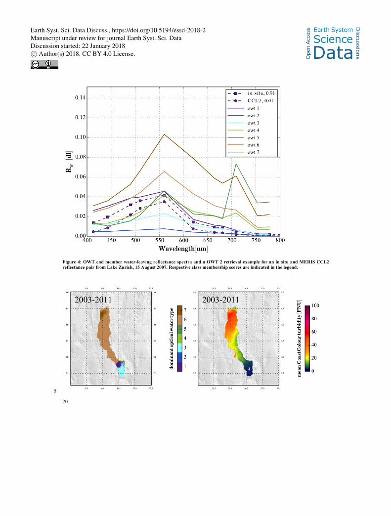
(Odermatt et al., 2012). Moore et al. (2014) developed an Optical Water Type classification (OWT) framework, which

supports the distinction of these different water types, and which is available as SNAP plugin (Peters, 2016). It assigns

water-leaving reflectance spectra to seven end members, which were identified through cluster analysis of in situ

measurements. Classes 1-3 represent clear or absorbing waters, classes 4-5 represent high phytoplankton and classes 6-7

represent high suspended mineral contents (Figure 4). The OWT algorithm depends on the accurate correction of 20

atmospheric effects (Eleveld et al., 2017), which was assessed by classifying 42 matchup pairs of in situ reflectance

measurements in 10 diverse lakes and MERIS water-leaving reflectance from various atmospheric corrections. Water-

leaving reflectance obtained with the CoastColour NN algorithm (description below) achieved the best agreement, in which

half the matchup pairs were assigned to the same OWT, and adjacent classes were assigned in 14 cases (Odermatt et al.,

2015a). In 5 out of the remaining 7 cases, the optically quite similar classes 1 and 3 are confused. This mismatch due to 25

differences between in situ measured and satellite observed reflectance is quite significant. However, when considering only

the separation between classes 1-3 and 4-7, and thus the feasibility of CHL-a retrieval based on the secondary reflectance

peak, the approach becomes very robust, with only 2 out of the 42 pairs being confused. The OWT maps therefore provide a

rough but robust indicator for CHL-a algorithm selection. Most lakes are relatively clearly dominated by either OWT 1-3 or

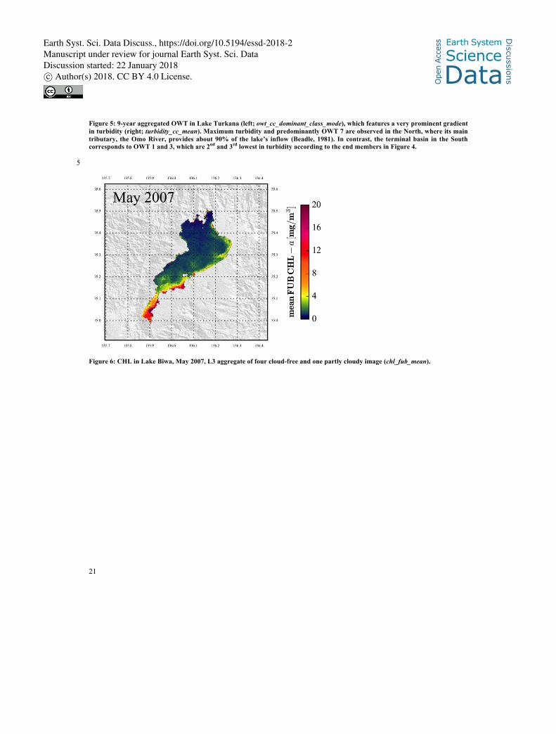
4-7, which makes the CHL-a product selection straightforward. In rare cases like Lake Turkana (Figure 5), such a selection 30

can only be made if either the lower or the upper end of the dynamic range is considered more relevant. Otherwise, it is

recommended to either split the lake perimeter or merge the CHL-a products e.g. by weighting them with turbidity levels.


Ope

n A

cces

s Earth System

Science

DataD

iscussio

ns


7

For the Diversity II production the Maximum Peak Height algorithm (MPH; Matthews et al., 2012) was developed further

and implemented in a SNAP operator (Block, 2016) because it outperformed other red-NIR reflectance peak algorithm in the

algorithm intercomparison study (Matthews and Odermatt, 2015; Odermatt et al., 2015a). It uses BRR in MERIS bands 6-10

and 14 for the retrieval of the red-NIR reflectance peak height and position, which allow for the identification of

cyanobacteria and eukaryote dominated pixels, water surface covering by cyanobacteria scum or floating vegetation, and 5

CHL-a quantification. Dedicated empirically calibrated equations are used for the retrieval of CHL-a concentrations in

eukaryote and cyanobacteria dominated waters. Technically, the algorithm is designed to cover the range of 0-1000 mg/m3

CHL-a. However, retrieval accuracy is significantly better for lakes that are predominantly OWT 4-7, namely eutrophic to

hypertrophic waters.

The FUB algorithm (Schroeder et al., 2007), named after the Free University of Berlin, is a bundle of dedicated NN 10

algorithms for CHL-a, Total Suspended Matter (TSM) and Coloured Dissolved Organic Matter (CDOM) retrieval from

MERIS L1B data, and a fourth NN that computes AOT at four wavelengths (440, 550, 670, 870 nm) and water-leaving

reflectance in all bands up to 708 nm, except at 680 nm. The algorithms are trained with radiative transfer simulations using

the Matrix Operator Model (MOMO; Fell and Fischer, 2001) covering CHL-a, TSM and CDOM concentration ranges of

0.05-50 mg/m3, 0.05-50 g/m3 and 0.005-1 m-1, respectively, and using MERIS bands 1-7, 9, 10 and 12-14 as input. The 15

training ranges are a severe limitation for global usage, but specific retrieval quality flags indicate for each of the four NN

algorithms if the input or output exceeds the training range. However for oligo- to eutrophic and in particular humic lakes,

which are commonly identified as OWT 1-3, the FUB algorithm’s CHL-a output outperformed all other candidates in the

intercomparison study (Odermatt et al., 2015a). Note that FUB uses shorter wavelengths that reach deeper into the water

column than MPH, which means that the two CHL-a products represent different depths and may not converge at 20

intermediate concentrations (ca. 10-30 mg/m3), where both algorithms produce valid results.

For the retrieval of TSM via particulate backscattering at 443 nm (bb_spm_443 in Figure 2) and turbidity, as well as water-

leaving reflectance input for the OWT classification, we used the CoastColour NN algorithm. Its architecture is based on the

approach described in Doerffer & Schiller (2007), with two dedicated NN systems performing atmospheric correction and

inherent optical properties retrieval (Doerffer, 2011; Ruescas et al., 2014). In contrast to earlier NN algorithms, the 25

CoastColour NN was trained with significantly larger concentration ranges, namely 0.03-1000 g/m3 TSM and 0.03-500

mg/m3 CHL. It was extensively validated with the CoastColour Round Robin data set (Nechad et al., 2015; available in

Pangaea) and lake in situ measurements (Odermatt et al., 2015a).

4.3. Post-processing and auxiliary data

The aggregation of L2 to L3 products (Figure 2) facilitates temporal binning and collocation in a common coordinate grid 30

with WGS 84 (EPSG 7030) coordinate system. Monthly aggregates are created using the input, output and aggregation

methods listed in Table 1, and the same aggregation methods are used to create yearly and 9-year aggregates from monthly

and yearly aggregates, respectively, which ensures that all months input aggregate periods are weighted equally even if the


Ope

n A

cces

s Earth System

Science

DataD

iscussio

ns


8

numbers of L2 available in these periods may differ strongly. Aggregation of biophysical parameters is done using the mean

of all valid nearest-neighbour input pixels for each output pixel, while the OWT L3 output layer consists of the most

frequently observed class value across all available input layers, using the lower class in the rare case of a draw.

Monthly, yearly and 9-year aggregates for each lake are saved in individual GeoTIFF files, and compressed in 13 ZIP files

representing 11 annual archives for the monthly aggregates, one archive for the yearly aggregate, and the 9-year aggregate. 5

These 13 ZIP archives are zipped again to make each lake available for download in a single file of up to 18.9 Gigabyte size

(Caspian Sea).

For extracting product statistics and for visualization of the products, a Python package is available at

https://github.com/odermatt/diversity. The scripts included in the package allow for creating spatial and temporal plots such

as shown in Section 5 (Figure 5 to Figure 12). They also feature the use of blacklists, e.g. to exclude all products with scarce 10

lake extent coverage from further analyses.

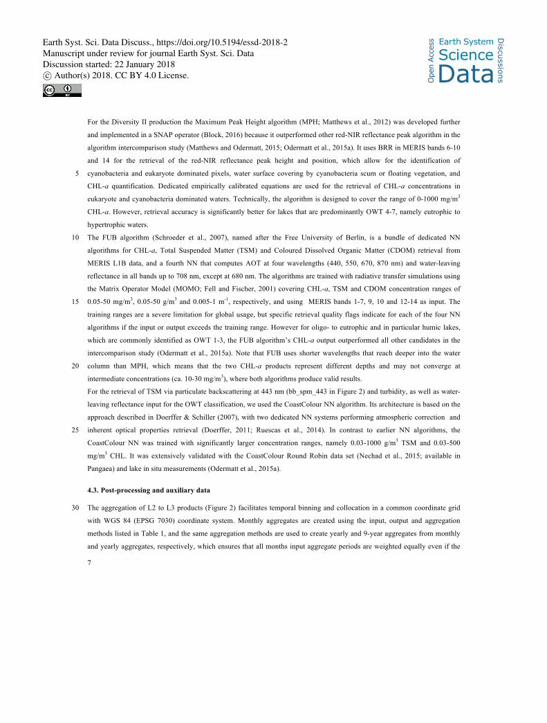
Table 1: Input, output and aggregation specifications for the monthly products.

Algorithm L2 input layer(s) Aggr. L3 output layer(s)

MPH chl: float [mg/m3] mean chl_mph: float [mg/m3]

FUB algal-2: float [mg/m3] mean chl_fub: float [mg/m3]

FUB yellow_subs: float [m-1] mean cdom_fub: float [m-1]

CoastColour bb_spm_443 mean tsm_cc: float [g/m3]

CoastColour turbidity: floating numbers [FTU] mean turbidity_cc: float [FTU]

MPH if CYANO_FLAG not FLOAT_FLAG: binary mean immersed_cyanobacteria: float [0-1, dl]

MPH if CYANO_FLAG and FLOAT_FLAG: binary mean floating_cyanobacteria: float [0-1, dl]

MPH if FLOAT_FLAG not CYANO_FLAG: binary mean floating_vegetation: float [0-1, dl]

OWT dominant_class: integer [1-7, dl] mode owt_cc_dominant_class: integer [1-7, dl]

ratio_490 See Section 4.1 mean shallow: binary

lswt_d See Section 3.3 none lswt_d_mean: float [deg. K]

lswt_n See Section 3.3 none lswt_d_mean: float [deg. K]

5. Results

The Diversity II water quality datasets were used for several lake-specific assessments, most prominently for indicating fish 15

assemblages and status assessments in Lake Vänern (Sweden; Sandström et al., 2016). Other use cases are described as

biodiversity stories and made available from www.diversity2.info. A summary of three selected examples verifies how the

remotely sensed parameters respond to spatio-temporally evident or relatively well-documented biophysical events.


Ope

n A

cces

s Earth System

Science

DataD

iscussio

ns


9

5.1. Lake Biwa

Lake Biwa is a monomictic lake northeast of Kyoto (Japan), up to 104 m deep and with a surface area of 658 km2 among the

smaller lakes in the dataset. The primary productivity of the lake is relatively low, but subject to strong spatial gradients that

are related to the distribution of residential and industrial areas, which are concentrated on the south-eastern shore and

responsible for increased riverine Nitrogen input (Ohte et al., 2010) that increase near-shore phytoplankton growth (Figure 5

6). In December 2007 investigations with an AUV (Autonomous Underwater Vehicle) revealed more than 2000 dead

organisms on the lake’s bottom, mostly endemic Isaza gobi fish and lake prawns. Low dissolved oxygen concentrations of

less than 1.0 mg/l near the lake bottom in November were identified as the main cause for an increased exposure of aquatic

organisms to heavy metals and the die-off (Itai et al., 2012; Kawanabe et al., 2012). Oxygen supply depends on wintertime

vertical mixing, which, aside from wind stress, depends on the vertical density gradients and thus thermal stratification. In 10

situ temperature profiles from the Lake Biwa Environmental Research Institute’s regular limnological survey program

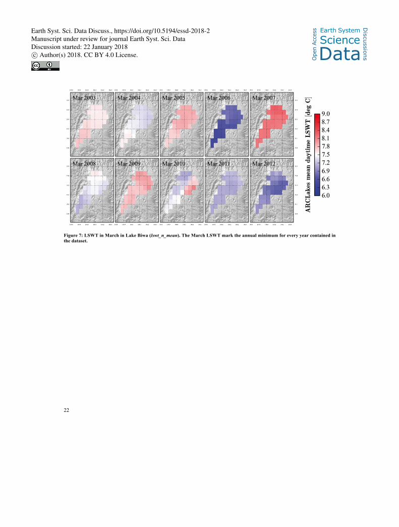
suggest that vertical mixing remained very weak in the winter of 2006/2007 (Kawanabe et al., 2012). Even though relating

surface to bottom temperatures is not without caveats, significantly higher LSWT with spatially averaged 8.2°C is observed

in March 2007 than in the other years (Figure 7), suggesting that minimal annual LSWT could be a valuable proxy for

vertical mixing in temperate lakes. 15

5.2. Lake Nicaragua

Lake Nicaragua/Cocibolca is the largest lake in Central America with a surface area of 7851 km2. It is polymictic with a

maximum and average depth of only 26 and 15 m, respectively. It is subject to prevalent ecological issues such as untreated

urban wastewater discharge and immissions from agriculture (soil erosion, fertilizer and pesticide immissions) and

aquacultures that introduce non-resident Tilapia species and possibly novel diseases. Moreover, the planned construction of 20

the Nicaragua Canal connecting the Caribbean Sea to the Pacific Ocean would bring about a significant shift in the lakes

ecological status, most directly through the excavation of a 27.6 m deep, 520 m wide and 286 km long waterway across the

centre of the shallow lake, which will strongly affect light availability within the water (Meyer and Huete-Pérez, 2014). In

spite of the limited availability of MERIS FR data over Latin America (Figure 1), it can contribute to estimating baseline

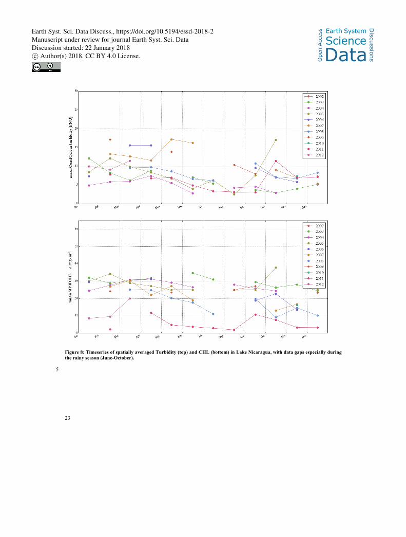
conditions prior to the intervention. Generally maximum and minimum turbidity occur around August and February, 25

respectively (Figure 8, top), within a range between 2-20 FNU. Outliers such as in October 2005 and May 2007 can occur

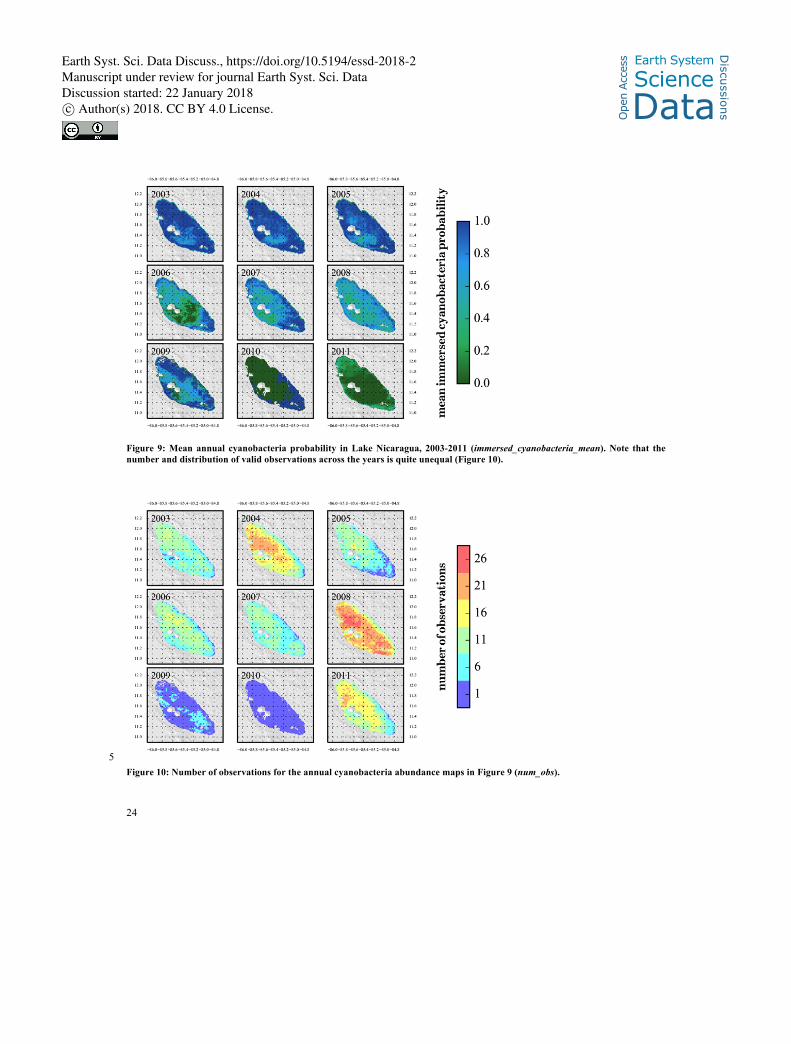
when only a small area of the lake is sampled. However, the 2011 turbidity peak in October is related to an extraordinary

shift from cyanobacteria to eucaryotic algae (Figure 9), which comes with significantly lower CHL concentrations

throughout the year from both the MPH (Figure 8, top) and the FUB algorithm (not shown), but also a second productivity

peak. Even though data continuity and in situ measurements are required for further interpretation, the available data 30

suggests that the lake was in a relatively unstable state at the end of the observation period.


Ope

n A

cces

s Earth System

Science

DataD

iscussio

ns


10

5.3. Lake Victoria

Lake Victoria is the second largest fresh water lake in the world and is situated in a shallow depression between the Great

Rift Valley and the western Albertine Rift, with a shoreline shared by Kenya, Uganda and Tanzania. It is up to 83 m deep,

eutrophic and light-limited (Hecky et al., 2010), and it’s thermocline is usually at around 30-40 m with complete mixing

occurring once a year (MacIntyre et al., 2014; Payne, 1986). About 80% of the water input to Lake Victoria are from direct 5

rainfall (Swenson and Wahr, 2009), and atmospheric deposition is the most important Phosphorous source in pelagic areas of

the main basin (Tamatamah et al., 2005). In contrast, the Nyanza Gulf (also known as Winam or Kavirondo Gulf), the lake’s

most distinctive morphological feature in the north-east, receives about 10% of the lake’s terrestrial inflow, and it was

concluded from ground measurements between March 2005 and March 2006 that the Nyanza Gulf even received

Phosphorous input from the main basin, in contrast to the paradigm that the gulf is a major contributor to the lake’s 10

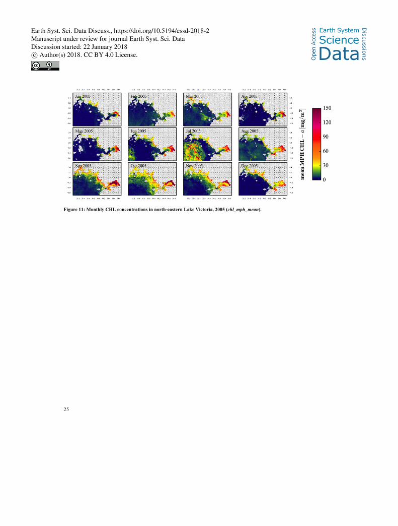
increasing nutrient enrichment (Gikuma-Njuru et al., 2013). As a matter of fact, MERIS observations confirm that the most

productive areas are located in the very east of the Gulf throughout 2005 (Figure 11) and for the first half of 2006 (not

shown). During this period, the CHL levels in the lake’s centre in July 2005 appear extraordinarily high. This observation

can be verified through a comparison with the number of available observations (2-7) and the abundance of immersed

cyanobacteria (0.4-1) in this area and month. This means that most parts of this cyanobacteria bloom were identified in 15

several observations.

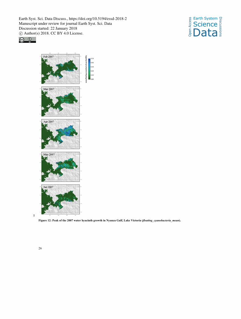
The Nyanza Gulf was also subject to intensive growth of water hyacinths (Eichhorna crassipes) in response to El Niño

precipitation anomalies in 1998 (Albright et al., 2004) and 2007 (Fusilli et al., 2013). Figure 12 displays the 2007

proliferation event according to Diversity II data. The hyacinths appear in floating_cyanobacteria_mean rather than the

expected floating_vegetation_mean, assumingly due to persistent cyanobacteria dominance in the Gulf. Given that Idepix is 20

likely to mask completely overgrown pixels as land (see Section 4.1), the remaining water pixels counted for the abundance

consist partly of immersed cyanobacteria, partly of floating eucaryotes. Despite these limitations and the fact that monthly

aggregates lack the spatial details of individual observations, the extent and course of the proliferation matches well with the

MODIS observations presented by Fusilli et al. (2013).

6. Discussion 25

6.1. Conclusions

The Diversity II dataset is the first globally representative, temporally resolved and methodologically consistent information

source for inland water quality dynamics from satellite Earth observations. It includes monthly, yearly and 9-year temporally

aggregated geophysical maps of various water quality parameters, which provide unprecedented possibilities for exploitation

at global and local scale. Global analyses are yet to be carried out, with caution to the limitations mentioned hereafter. At 30

local scale, several case studies demonstrated how the data could effectively contribute to traditional investigations of lake


Ope

n A

cces

s Earth System

Science

DataD

iscussio

ns


11

specific processes and events. The Diversity II product user handbook (Odermatt et al., 2015b) helps to improve such

interpretation of remotely sensed data by providing background knowledge of acquisition and retrieval methods, and Python

scripts are available that facilitate standard information extraction and visualization from the individual GeoTIFF files.

The methods used for producing the Diversity II dataset represent the state-of-the art at the end of the ENVISAT era. It is a

major asset of Earth observation that productions from L1 observations can be repeated as improved methods become 5

available, so there is no doubt that the methods in use for Diversity II will be improved and overhauled in the future. Several

lessons were learned for such repeated productions, some of them involving challenges for future research. For example, the

binary identification of optically shallow waters and floating lake ice have received relatively little attention in recent years,

but under certain circumstances they have much larger effects on the final product accuracy than retrieval algorithms. Our

method for the identification of clouds, land and mixed pixels is more advanced, but it remains critical for all partly cloudy 10

situations. Therefore, the development of such methods should receive much more attention, relative to the number of

retrieval algorithms that were developed in recent years. The latest generation of retrieval algorithms will be based on further

advanced water types (Spyrakos et al., n.d.) and ensemble approaches that account for the selection of multiple algorithms’

estimates (as e.g. left to the user with chl_mph_mean/chl_fub_mean). Finally, new approaches are needed for the

consolidation of such increasingly large geospatial datasets, and for the extraction of relevant information, which is still 15

mostly based on lake-specific knowledge.

6.2. Limitations

Areas of melting lake ice are optically very similar to water, and the false retention of a lake ice covered pixel by the Idepix

algorithm can lead to highly irregular constituent estimates. Indicators for such cases are the seasonal timing, sharp linear

features in water constituent products, indicating lake ice borders or cracks, and very low values in mean LSWT. Auxiliary 20

data from the NOAA/NSDIC Global Lake and River Ice Phenology Database could also help with the identification. A

procedure to fix monthly products that are affected by melting lake ice artefacts using the BEAM L3 binner is described in

Odermatt et al. (2015b).

Ephemeral (also intermittent or seasonal) lakes as well as other lakes and reservoirs that significantly change their extent

over time are usually not well represented because the lakes’ areas are clipped to the extent of the SWBD in February 2000. 25

Their change in extent also complicates the identification of shallow water areas in a way that makes our approach based on

temporally consistent spectroradiometric properties inapplicable. Therefore ratio_490 thresholds for such lakes were set to

0.0 to disable shallow water identification. Furthermore, many of these lakes are subject to very high salinity levels and other

typical habitat properties that favour extraordinary types of water constituents and accordingly bio-optical properties, which

can significantly affect the validity of the water quality products. Particular care is thus needed when a lakes’ product layer 30

extent is significantly smaller than expected.


Ope

n A

cces

s Earth System

Science

DataD

iscussio

ns


12

The relative abundances in the floating_vegetation and floating_cyanobacteria layers include only pixels that passed the

foregoing Idepix masking. This means that especially very densely covered water pixels are previously identified as land

pixels and not counted, resulting in an overall underestimation of abundances.

7. References

Albright, T., Moorhouse, T. G. and McNabb, T. J.: The Rise and Fall of Water Hyacinth in Lake Victoria and the Kagera 5

River Basin, 1989-2001, Journal of Aquatic Plant Management, 42, 73–84, 2004.

Alvera-Azcárate, A., Barth, A., Rixen, M. and Beckers, J. M.: Reconstruction of incomplete oceanographic data sets using

empirical orthogonal functions: application to the Adriatic Sea surface temperature, Ocean Modelling, 9(4), 325–346,

doi:10.1016/j.ocemod.2004.08.001, 2005.

Beadle, L. C.: The inland waters of tropical Africa. An introduction to tropical limnology., Longman Group Limited, 10

London, England., 1981.

Block, T.: diversity-mph-chl Operator, Brockmann Consult, Geesthacht, Germany. [online] Available from:

https://github.com/bcdev/beam-diversity-auxdata/tree/master/diversity-mph-chl, 2016.

Bourg, L. and Etanchaud, F.: The AMORGOS MERIS CFI (Accurate MERIS Ortho-Rectified Geolocation Operational

Software), Software User Manual and Interface Control Document, ACRI-ST, Sophia-Antipolis, France. [online] Available 15

from: earth.esa.int/services/amorgos/download/Amorgos_ICD-SUM_3.0a.pdf, 2007.

Cannizzaro, J. P. and Carder, K.: Estimating chlorophyll a concentrations from remote-sensing reflectance in optically

shallow waters, Remote Sensing of Environment, 101(1), 13, 2006.

Crétaux, J.-F., Jelinski, W., Calmant, S., Kouraev, A., Vuglinski, V., Bergé-Nguyen, M., Gennero, M.-C., Nino, F., Rio, R.

A. D., Cazenave, A. and Maisongrande, P.: SOLS: A lake database to monitor in the Near Real Time water level and storage 20

variations from remote sensing data, Advances in Space Research, 47(9), 1497–1507,

doi:http://dx.doi.org/10.1016/j.asr.2011.01.004, 2011.

Danne, O.: beam-idepix Operator, Brockmann Consult, Geesthacht, Germany. [online] Available from:

https://github.com/bcdev/beam-idepix, 2016.

Doerffer, R.: Alternative Atmospheric Correction Procedure for Case 2 Water Remote Sensing using MERIS, MERIS 25

ATBD, Helmholtz Zentrum Geesthacht, Geesthacht, Germany. [online] Available from:

https://earth.esa.int/documents/700255/2042855/MERIS_ATBD_2.25_v1.0+-+2011.pdf, 2011.

Doerffer, R. and Schiller, H.: The MERIS Case 2 water algorithm, International Journal of Remote Sensing, 28(3–4), 517–

535, doi:10.1080/01431160600821127, 2007.

Eleveld, M. A., Ruescas, A. B., Hommersom, A., Moore, T. S., Peters, S. W. M. and Brockmann, C.: An Optical 30

Classification Tool for Global Lake Waters, Remote Sensing, 9(5), doi:10.3390/rs9050420, 2017.


Ope

n A

cces

s Earth System

Science

DataD

iscussio

ns


13

Fell, F. and Fischer, J.: Numerical simulation of the light field in the atmosphere–ocean system using the matrix-operator

method, Journal of Quantitative Spectroscopy and Radiative Transfer, 69(3), 351–388, doi:10.1016/S0022-4073(00)00089-3,

2001.

Fomferra, N. and Brockmann, C.: BEAM - The ENVISAT MERIS and AATSR Toolbox, in MERIS (A)ATSR Workshop

2005, vol. 597, p. 13.1., 2005. 5

Fomferra, N., Böttcher, M., Zühlke, M., Brockmann, C. and Kwiatkowska, E.: Calvalus: Full-mission EO cal/val, processing

and exploitation services, in 2012 IEEE International Geoscience and Remote Sensing Symposium, pp. 5278–5281., 2012.

Fusilli, L., Collins, M. O., Laneve, G., Palombo, A., Pignatti, S. and Santini, F.: Assessment of the abnormal growth of

floating macrophytes in Winam Gulf (Kenya) by using MODIS imagery time series, International Journal of Applied Earth

Observation and Geoinformation, 20(0), 33–41, doi:10.1016/j.jag.2011.09.002, 2013. 10

Gikuma-Njuru, P., Hecky, R. E., Guildford, S. J. and MacIntyre, S.: Spatial variability of nutrient concentrations, fluxes, and

ecosystem metabolism in Nyanza Gulf and Rusinga Channel, Lake Victoria (East Africa), Limnology and Oceanography,

58(3), 774–789, doi:10.4319/lo.2013.58.3.0774, 2013.

Gitelson, A.: The peak near 700 nm on radiance spectra of algae and water: relationships of its magnitude and position with

chlorophyll concentration, International Journal of Remote Sensing, 13(17), 3367 – 3373, 1992. 15

Gleick, P. H.: Water Resources, in Encyclopaedia of Climate and Weather, vol. 2, edited by S. H. Schneider, pp. 817–823,

Oxford University Press, New York, United States. [online] Available from:

http://www.oxfordreference.com/view/10.1093/acref/9780199765324.001.0001/acref-9780199765324, 1996.

Gons, H. J.: Optical Teledetection of Chlorophyll a in Turbid Inland Waters, Environmental Science & Technology, 33(7),

1127–1132, doi:10.1021/es9809657, 1999. 20

Gower, J. F. R., Doerffer, R. and Borstad, G. A.: Interpretation of the 685nm peak in water-leaving radiance spectra in terms

of fluorescence, absorption and scattering, and its observation by MERIS, International Journal of Remote Sensing, 20(9),

1771–1786, 1999.

Hecky, R. E., Mugidde, R., Ramlal, P. S., Talbot, M. R. and Kling, G. W.: Multiple stressors cause rapid ecosystem change

in Lake Victoria, Freshwater Biology, 55, 19–42, doi:10.1111/j.1365-2427.2009.02374.x, 2010. 25

Itai, T., Hayase, D., Hyobu, Y., Hirata, S. H., Kumagai, M. and Tanabe, S.: Hypoxia-Induced Exposure of Isaza Fish to

Manganese and Arsenic at the Bottom of Lake Biwa, Japan: Experimental and Geochemical Verification, Environ. Sci.

Technol., 46(11), 5789–5797, doi:10.1021/es300376y, 2012.

Kawanabe, H., Nishino, M. and Maehata, M.: Lake Biwa: Interactions between Nature and People, Springer, Dordrecht,

Netherlands., 2012. 30

Kiefer, I., Odermatt, D., Anneville, O., Wüest, A. and Bouffard, D.: Application of remote sensing for the optimization of in-

situ sampling for monitoring of phytoplankton abundance in a large lake, Science of The Total Environment, 527–528(0),

493–506, doi:10.1016/j.scitotenv.2015.05.011, 2015.


Ope

n A

cces

s Earth System

Science

DataD

iscussio

ns


14

Kirches, G., Krueger, O., Boettcher, M., Bontemps, S., Lamarche, C., Verheggen, A., Lembrée, C., Radoux, J. and

Defourny, P.: Algorithm Theoretical Basis Document v2.3, ESA CCI Project LandCover. [online] Available from:

http://www.esa-landcover-cci.org/?q=documents#, 2013.

Lehner, B. and Döll, P.: Development and validation of a global database of lakes, reservoirs and wetlands, Journal of

Hydrology, 296(1–4), 1–22, 2004. 5

M. Santoro and U. Wegmüller: Multi-temporal Synthetic Aperture Radar Metrics Applied to Map Open Water Bodies, IEEE

Journal of Selected Topics in Applied Earth Observations and Remote Sensing, 7(8), 3225–3238,

doi:10.1109/JSTARS.2013.2289301, 2014.

MacCallum, S. and Merchant, C.: ATSR Reprocessing for Climate Lake Surface Temperature: ARC-Lake Algorithm

Theoretical Basis Document, Univ. of Edinburgh, Edinburgh, Scotland. [online] Available from: 10

http://www.geos.ed.ac.uk/arclake/ARC-Lake-ATBD-v1.4.pdf, 2013.

MacCallum, S. and Merchant, C.: ARC-Lake Data Product Description, Univ. of Edinburgh, Edinburgh, Scotland. [online]

Available from: www.laketemp.net/home/ARCLake_DPD_v3.pdf, 2014.

MacCallum, S. N. and Merchant, C. J.: Surface water temperature observations of large lakes by optimal estimation,

Canadian Journal of Remote Sensing, 38(01), 25–45, doi:10.5589/m12-010, 2012. 15

MacIntyre, S., Romero, J. R., Silsbe, G. M. and Emery, B. M.: Stratification and horizontal exchange in Lake Victoria, East

Africa, Limnology and Oceanography, 59(6), 1805–1838, doi:10.4319/lo.2014.59.6.1805, 2014.

Matthews, M. W.: A current review of empirical procedures of remote sensing in inland and near-coastal transitional waters,

International Journal of Remote Sensing, 32(21), 6855–6899, doi:10.1080/01431161.2010.512947, 2011.

Matthews, M. W. and Odermatt, D.: Improved algorithm for routine monitoring of cyanobacteria and eutrophication in 20

inland and near-coastal waters, Remote Sensing of Environment, 156, 374–382, doi:10.1016/j.rse.2014.10.010, 2015.

Matthews, M. W., Bernard, S. and Robertson, L.: An algorithm for detecting trophic status (chlorophyll-a), cyanobacterial-

dominance, surface scums and floating vegetation in inland and coastal waters, Remote Sensing of Environment, 124(0),

637–652, doi:10.1016/j.rse.2012.05.032, 2012.

Meyer, A. and Huete-Pérez, J. A.: Nicaragua Canal could wreak environmental ruin, Nature, 506(7488), 287–289, 2014. 25

Mironov, D.: Parameterization of lakes in numerical weather prediction. Description of a lake model, COSMO Technical

Report, No. 11, Deutscher Wetterdienst, Offenbach am Main, Germany. [online] Available from: http://www.cosmo-

model.org/content/model/documentation/techReports/docs/techReport11.pdf, 2008.

Mobley, C. D., Stramski, D., Bisset, W. P. and Boss, E.: Optical modeling of ocean water: Is the case 1 - case 2 classification

still useful?, Oceanography, 17(2), 60–67, 2004. 30

Moore, T. S., Dowell, M. D., Bradt, S. and Ruiz Verdu, A.: An optical water type framework for selecting and blending

retrievals from bio-optical algorithms in lakes and coastal waters, Remote Sensing of Environment, 143(0), 97–111,

doi:10.1016/j.rse.2013.11.021, 2014.

Morel, A. and Prieur, L.: Analysis of Variations in Ocean Color, Limnology and Oceanography, 22(4), 709–722, 1977.


Ope

n A

cces

s Earth System

Science

DataD

iscussio

ns


15

Nechad, B., Ruddick, K., Schroeder, T., Oubelkheir, K., Blondeau-Patissier, D., Cherukuru, N., Brando, V., Dekker, A.,

Clementson, L., Banks, A. C., Maritorena, S., Werdell, P. J., Sá, C., Brotas, V., Caballero de Frutos, I., Ahn, Y.-H., Salama,

S., Tilstone, G., Martinez-Vicente, V., Foley, D., McKibben, M., Nahorniak, J., Peterson, T., Siliò-Calzada, A., Röttgers, R.,

Lee, Z., Peters, M. and Brockmann, C.: CoastColour Round Robin data sets: a database to evaluate the performance of

algorithms for the retrieval of water quality parameters in coastal waters, Earth System Science Data, 7(2), 319–348, 5

doi:10.5194/essd-7-319-2015, 2015.

Odermatt, D., Gitelson, A., Brando, V. E. and Schaepman, M. E.: Review of constituent retrieval in optically deep and

complex waters from satellite imagery, Remote Sensing of Environment, 118, 116–126, doi:10.1016/j.rse.2011.11.013,

2012.

Odermatt, D., Gangkofner, U., Ratzmann, G., Ruescas, A. B., Stelzer, K., Philipson, P. and Brockmann, C.: Algorithm 10

Theoretic Baseline Document v2.4, ESA DUE Project Diversity II. [online] Available from:

www.diversity2.info/products/documents/, 2015a.

Odermatt, D., Brito, J., Philipson, P., Hahn, N. and Brockmann, C.: Products User Handbook Inland Waters v2.1, ESA DUE

Project Diversity II. [online] Available from: http://www.diversity2.info/products/documents/, 2015b.

Ohte, N., Tayasu, I., Kohzu, A., Yoshimizu, C., Osaka, K., Makabe, A., Koba, K., Yoshida, N. and Nagata, T.: Spatial 15

distribution of nitrate sources of rivers in the Lake Biwa watershed, Japan: Controlling factors revealed by nitrogen and

oxygen isotope values, Water Resources Research, 46(7), W07505, doi:10.1029/2009WR007871, 2010.

Palmer, S. C. J., Odermatt, D., Hunter, P. D., Brockmann, C., Présing, M., Balzter, H. and Tóth, V. R.: Satellite remote

sensing of phytoplankton phenology in Lake Balaton using 10 years of MERIS observations, Remote Sensing of

Environment, 158(0), 441–452, doi:10.1016/j.rse.2014.11.021, 2015. 20

Payne, A. I.: The Ecology of Tropical Lakes and Rivers, John Wiley & Sons Ltd., New York, United States., 1986.

Peters, M.: beam-owt-classification Operator, Brockmann Consult, Geesthacht, Germany. [online] Available from:

https://github.com/bcdev/coastcolour/tree/master/beam-owt-classification, 2016.

Politi, E., MacCallum, S., Cutler, M. E. J., Merchant, C. J., Rowan, J. S. and Dawson, T. P.: Selection of a network of large

lakes and reservoirs suitable for global environmental change analysis using Earth Observation, International Journal of 25

Remote Sensing, 37(13), 3042–3060, doi:10.1080/01431161.2016.1192702, 2016.

Rast, M., Bezy, J. L. and Bruzzi, S.: The ESA Medium Resolution Imaging Spectrometer MERIS a review of the instrument

and its mission, International Journal of Remote Sensing, 20(9), 1681–1702, doi:10.1080/014311699212416, 1999.

Ruescas, A. B., Brockmann, C., Stelzer, K., Tilstone, G. H. and Beltran, J.: DUE CoastColour Validation Report,

Brockmann Consult, Geesthacht, Germany. [online] Available from: http://www.coastcolour.org/documents/DEL-30

27%20Validation%20Report_v1.pdf, 2014.

Sandström, A., Philipson, P., Asp, A., Axenrot, T., Kinnerbäck, A., Ragnarsson-Stabo, H. and Holmgren, K.: Assessing the

potential of remote sensing-derived water quality data to explain variations in fish assemblages and to support fish status

assessments in large lakes, Hydrobiologia, 780(1), 71–84, doi:10.1007/s10750-016-2784-9, 2016.


Ope

n A

cces

s Earth System

Science

DataD

iscussio

ns


16

Santer, R., Carrere, V., Dubuisson, P. and Roger, J. C.: Atmospheric correction over land for MERIS, International Journal

of Remote Sensing, 20(9), 1819–1840, doi:10.1080/014311699212506, 1999.

Sayers, M. J., Grimm, A. G., Shuchman, R. A., Deines, A. M., Bunnell, D. B., Raymer, Z. B., Rogers, M. W., Woelmer, W.,

Bennion, D. H., Brooks, C. N., Whitley, M. A., Warner, D. M. and Mychek-Londer, J.: A new method to generate a high-

resolution global distribution map of lake chlorophyll, International Journal of Remote Sensing, 36(7), 1942–1964, 5

doi:10.1080/01431161.2015.1029099, 2015.

Schroeder, T., Schaale, M. and Fischer, J.: Retrieval of atmospheric and oceanic properties from MERIS measurements: A

new Case-2 water processor for BEAM, International Journal of Remote Sensing, 28(24), 5627 – 5632, 2007.

Sectretariat of the Convention on Biological Diversity: Global Biodiversity Outlook 3, Montréal, Canada. [online] Available

from: www.cbd.int/gbo3/, 2010. 10

Slater, J. A., Garvey, G., Johnston, C., Haase, J., Heady, B., Kroenung, G. and Little, J.: The SRTM Data “Finishing”

Process and Products, Photogrammetric Engineering & Remote Sensing, 72(3), 237–247, doi:10.14358/PERS.72.3.237,

2006.

Spyrakos, E., O’Donnell, R., Hunter, P. D., Miller, C., Scott, M., Simis, S. G. H., Neil, C., Barbosa, C. C. F., Binding, C. E.,

Bradt, S., Bresciani, M., Dall’Olmo, G., Giardino, C., Gitelson, A. A., Kutser, T., Li, L., Matsushita, B., Martinez-Vicente, 15

V., Matthews, M. W., Ogashawara, I., Ruiz-Verdú, A., Schalles, J. F., Tebbs, E., Zhang, Y. and Tyler, A. N.: Optical types

of inland and coastal waters, Limnology and Oceanography, n/a-n/a, doi:10.1002/lno.10674, n.d.

Swenson, S. and Wahr, J.: Monitoring the water balance of Lake Victoria, East Africa, from space, Journal of Hydrology,

370(1), 163–176, doi:10.1016/j.jhydrol.2009.03.008, 2009.

Tamatamah, R. A., Hecky, R. E. and Duthie, H.: The atmospheric deposition of phosphorus in Lake Victoria (East Africa), 20

Biogeochemistry, 73(2), 325–344, doi:10.1007/s10533-004-0196-9, 2005.

Verpoorter, C., Kutser, T., Seekell, D. A. and Tranvik, L. J.: A global inventory of lakes based on high-resolution satellite

imagery, Geophysical Research Letters, 41(18), 6396–6402, doi:10.1002/2014GL060641, 2014.


Ope

n A

cces

s Earth System

Science

DataD

iscussio

ns


17

Figure 1: Global density maps for the bulk reprocessed MERIS FR dataset in the years 2002-2012, and distribution of the 340 lakes available in the Diversity II water quality dataset (bottom right).


Ope

n A

cces

s Earth System

Science

DataD

iscussio

ns


18

Figure 2: The CaLimnos v1 processing chain for inland waters. Coloration indicates algorithms and downstream processes (white), input and auxiliary data (dark grey), intermediate products (light grey) and output products (blue).

chl_mphchl_fub

cdom_fubtsm_cc

turbidity_ccimmersed_cyanobacteria

floating_cyanobacteriafloating_vegetation

owt_cc_dominant_classshallow

Leve

l 1A

uxili

ary

data

Leve

l 2Le

vel 3

Aux

iliar

y da

ta

MERIS FSGL1B

chlCYANO_FLAGFLOAT_FLAG

ADJ_FLAG

FUBMPH CoastColour

algal-2 yellow_subsCHL_OUTYEL_OUT

bb_spm_443turbidityINVALID

LAND MIXEDPIXEL

CLOUD CLOUD_BUFFER CLOUD_SHADOW

aggregate

AATSRARC-Lake monthly

lswt_dlswt_n

collocate

rectangular filter

ASARLC SAR-WB

maximum_extent

vectorize

D2-Sites inland watercoord, names, shallow_thres

intersectD2-Polygons300 polygons

maximum_extent

SRTMSWBD

timed_extent

D2-Shallowstatic map

shallow

ratio490OWT

Idepix

dominant_class

D2-Waterqualitymonthly/yearly/9-year

chl_mphchl_fub

cdom_fubtsm_cc



owt_cc_dominant_classshallowlswt_dlswt_n

D2-Timeserieslake averages

chl_mphchl_fub

cdom_fubtsm_cc



owt_cc_dominant_classshallowlswt_dlswt_n

water_level

aggregate

brr_1-10 brr_12-14


Ope

n A

cces

s Earth System

Science

DataD

iscussio

ns


19

Figure 3: Shallow water flagging for the Beaver Island Archipelago in the North of Lake Michigan. Top: Sentinel-2A true colour image, 8 May 2017. Centre: ratio_490 from MERIS data, acquired in May-October 2008. Bottom: Shallow water mask for 5 ratio_490 with a threshold of 0.65 on top of the CHL layer for October 2011 as contained in the product layer shallow. Bathymetry data provided by NOAA-NCEI.


Ope

n A

cces

s Earth System

Science

DataD

iscussio

ns


20

Figure 4: OWT end member water-leaving reflectance spectra and a OWT 2 retrieval example for an in situ and MERIS CCL2 reflectance pair from Lake Zurich, 15 August 2007. Respective class membership scores are indicated in the legend.

5


Ope

n A

cces

s Earth System

Science

DataD

iscussio

ns


21

Figure 5: 9-year aggregated OWT in Lake Turkana (left; owt_cc_dominant_class_mode), which features a very prominent gradient in turbidity (right; turbidity_cc_mean). Maximum turbidity and predominantly OWT 7 are observed in the North, where its main tributary, the Omo River, provides about 90% of the lake’s inflow (Beadle, 1981). In contrast, the terminal basin in the South corresponds to OWT 1 and 3, which are 2nd and 3rd lowest in turbidity according to the end members in Figure 4.

5

Figure 6: CHL in Lake Biwa, May 2007, L3 aggregate of four cloud-free and one partly cloudy image (chl_fub_mean).


Ope

n A

cces

s Earth System

Science

DataD

iscussio

ns


22

Figure 7: LSWT in March in Lake Biwa (lswt_n_mean). The March LSWT mark the annual minimum for every year contained in the dataset.


Ope

n A

cces

s Earth System

Science

DataD

iscussio

ns


23

Figure 8: Timeseries of spatially averaged Turbidity (top) and CHL (bottom) in Lake Nicaragua, with data gaps especially during the rainy season (June-October).

5


Ope

n A

cces

s Earth System

Science

DataD

iscussio

ns


24

Figure 9: Mean annual cyanobacteria probability in Lake Nicaragua, 2003-2011 (immersed_cyanobacteria_mean). Note that the number and distribution of valid observations across the years is quite unequal (Figure 10).

5 Figure 10: Number of observations for the annual cyanobacteria abundance maps in Figure 9 (num_obs).


Ope

n A

cces

s Earth System

Science

DataD

iscussio

ns


25

Figure 11: Monthly CHL concentrations in north-eastern Lake Victoria, 2005 (chl_mph_mean).


Ope

n A

cces

s Earth System

Science

DataD

iscussio

ns


26

5 Figure 12: Peak of the 2007 water hyacinth growth in Nyanza Gulf, Lake Victoria (floating_cyanobacteria_mean).


Ope

n A

cces

s Earth System

Science

DataD

iscussio

ns


Documents

1,2 Discussion started: 22 January 2018 c Author(s) … · Manuscript under review for journal Earth Syst. Sci. Data Discussion started: 22 January 2018 c. 4