Embed Size (px)
DESCRIPTION
b
Citation preview

CALCULUS II:
Multi-variable Calculus
Lecture notes and Workbook for 4CCM112A
Dr Sakura Schafer-Nameki
King’s College London
Based on lecture notes by
G.M.T. Watts, F.A. Rogers and S.G. Scott
January 6, 2015
2
CONTENTS 3
Contents
1 Introduction 7
1.1 Course outline . . . . . . . . . . . . . . . . . . . . . . . . . . . . . . . . . . . . . . 7
2 Functions R → Rn 10
2.1 Curves, paths and parametrisations . . . . . . . . . . . . . . . . . . . . . . . . . . . 10
2.1.1 Paths and Vector-valued Functions . . . . . . . . . . . . . . . . . . . . . . . 12
2.1.2 Parameterisations of curves . . . . . . . . . . . . . . . . . . . . . . . . . . . 15
2.2 Differentiation of paths . . . . . . . . . . . . . . . . . . . . . . . . . . . . . . . . . . 19
2.3 Tangent Lines . . . . . . . . . . . . . . . . . . . . . . . . . . . . . . . . . . . . . . . 21
2.4 Taylor’s Theorem for Vector-valued Functions . . . . . . . . . . . . . . . . . . . . . 24
2.5 Product rules for differentiation of paths . . . . . . . . . . . . . . . . . . . . . . . . 26
3 Functions Rm → R 31
3.1 Graphs of scalar functions . . . . . . . . . . . . . . . . . . . . . . . . . . . . . . . . 31
3.2 Directional derivatives . . . . . . . . . . . . . . . . . . . . . . . . . . . . . . . . . . 38
3.3 Partial derivatives . . . . . . . . . . . . . . . . . . . . . . . . . . . . . . . . . . . . 42
3.4 A formula for the tangent plane to a surface . . . . . . . . . . . . . . . . . . . . . . 45
3.5 The gradient of a scalar function . . . . . . . . . . . . . . . . . . . . . . . . . . . . 46
3.5.1 Alternative formula for the tangent plane to a surface . . . . . . . . . . . . 50
3.6 The rate of change of a function f : Rm −→ R1 . . . . . . . . . . . . . . . . . . . . 51
3.7 Taylor’s Theorem in Two Variables . . . . . . . . . . . . . . . . . . . . . . . . . . . 53
3.8 Maxima and minima of a function . . . . . . . . . . . . . . . . . . . . . . . . . . . 57
4 Functions Rm → Rn:
chain rule, grad, div and curl 63
4.1 The chain rule for derivatives . . . . . . . . . . . . . . . . . . . . . . . . . . . . . . 63
4.1.1 The Chain rule for functions R2 → R2 in matrix form . . . . . . . . . . . . 66
4.1.2 The chain rule and paths . . . . . . . . . . . . . . . . . . . . . . . . . . . . 68
4.2 Surfaces as level sets, the chain rule and tangent planes . . . . . . . . . . . . . . . 69
4.2.1 Level surfaces . . . . . . . . . . . . . . . . . . . . . . . . . . . . . . . . . . . 69
4.2.2 Level Curves . . . . . . . . . . . . . . . . . . . . . . . . . . . . . . . . . . . 76
4.3 Vector Fields . . . . . . . . . . . . . . . . . . . . . . . . . . . . . . . . . . . . . . . 77
4.4 Derivatives of vector fields: Div and Curl . . . . . . . . . . . . . . . . . . . . . . . 78
4 CONTENTS
4.5 Identities for ∇ . . . . . . . . . . . . . . . . . . . . . . . . . . . . . . . . . . . . . . 80
4.6 Formulae for the tangent plane to a surface . . . . . . . . . . . . . . . . . . . . . . 82
4.7 Tests for integrability of vector fields . . . . . . . . . . . . . . . . . . . . . . . . . . 83
4.7.1 Can v be written as the gradient of a scalar function? . . . . . . . . . . . . 83
4.7.2 Can v be written as the curl of a vector field? . . . . . . . . . . . . . . . . . 83
4.8 Miscellaneous exercises . . . . . . . . . . . . . . . . . . . . . . . . . . . . . . . . . . 84
4.9 Cross-products and the ǫ-tensor . . . . . . . . . . . . . . . . . . . . . . . . . . . . . 86
5 Application: Extremising with extra conditions 90
5.1 Extrema with extra conditions . . . . . . . . . . . . . . . . . . . . . . . . . . . . . 90
5.2 The Lagrange Multiplier Theorem . . . . . . . . . . . . . . . . . . . . . . . . . . . 94
6 FTC for Curves: Dimension One 97
6.1 Integrals of Scalar Functions over Curves . . . . . . . . . . . . . . . . . . . . . . . 97
6.2 Arc length . . . . . . . . . . . . . . . . . . . . . . . . . . . . . . . . . . . . . . . . . 100
6.3 Line integrals . . . . . . . . . . . . . . . . . . . . . . . . . . . . . . . . . . . . . . . 103
6.4 FTC I . . . . . . . . . . . . . . . . . . . . . . . . . . . . . . . . . . . . . . . . . . . 107
7 FTC for Surfaces: Flat Space 110
7.1 Integrals over Surfaces: Case (I) flat space . . . . . . . . . . . . . . . . . . . . . . . 110
7.2 More general regions . . . . . . . . . . . . . . . . . . . . . . . . . . . . . . . . . . . 115
7.2.1 Areas of regions from double integrals . . . . . . . . . . . . . . . . . . . . . 118
7.3 Changing variables . . . . . . . . . . . . . . . . . . . . . . . . . . . . . . . . . . . . 118
7.4 Polar coordinates . . . . . . . . . . . . . . . . . . . . . . . . . . . . . . . . . . . . . 123
7.5 FTC II: Green’s theorem . . . . . . . . . . . . . . . . . . . . . . . . . . . . . . . . . 127
8 FTC for Surfaces: Curved Space 131
8.1 Integrals over Surfaces: Case (II) curved space . . . . . . . . . . . . . . . . . . . . 131
8.2 Parameterisations of Surfaces: Coordinates . . . . . . . . . . . . . . . . . . . . . . 132
8.2.1 Parametrising graph-surfaces . . . . . . . . . . . . . . . . . . . . . . . . . . 137
8.3 The fundamental vector product of a surface . . . . . . . . . . . . . . . . . . . . . 139
8.4 Evaluating Surface Integrals and Surface area . . . . . . . . . . . . . . . . . . . . . 143
8.5 Surface Integrals of Vector Fields . . . . . . . . . . . . . . . . . . . . . . . . . . . . 146
8.6 Stokes’ theorem . . . . . . . . . . . . . . . . . . . . . . . . . . . . . . . . . . . . . . 150
8.7 Miscellaneous Exercises . . . . . . . . . . . . . . . . . . . . . . . . . . . . . . . . . 155
9 FTC in Dimension Three: the Divergence Theorem 156
9.1 Triple Integrals: integrals over regions of flat 3-space . . . . . . . . . . . . . . . . . 156
9.2 Special Coordinate Systems in R3. . . . . . . . . . . . . . . . . . . . . . . . . . . . 162
9.2.1 Cylindrical Polar Coordinates: (r, θ, z) . . . . . . . . . . . . . . . . . . . . . 162
9.2.2 Spherical Polar Coordinates: (ρ, θ, φ) . . . . . . . . . . . . . . . . . . . . . . 162
9.3 Changing variables . . . . . . . . . . . . . . . . . . . . . . . . . . . . . . . . . . . . 163
9.4 FTC III: The Divergence Theorem . . . . . . . . . . . . . . . . . . . . . . . . . . . 169
CONTENTS 5
A Revision notes on vectors 174
A.1 Vectors in R2 . . . . . . . . . . . . . . . . . . . . . . . . . . . . . . . . . . . . . . . 174
A.1.1 Definitions . . . . . . . . . . . . . . . . . . . . . . . . . . . . . . . . . . . . 174
A.1.2 Unit vectors . . . . . . . . . . . . . . . . . . . . . . . . . . . . . . . . . . . . 174
A.1.3 The length of a vector . . . . . . . . . . . . . . . . . . . . . . . . . . . . . . 174
A.1.4 The scalar or dot product . . . . . . . . . . . . . . . . . . . . . . . . . . . . 175
A.2 Vectors in R3 . . . . . . . . . . . . . . . . . . . . . . . . . . . . . . . . . . . . . . . 175
A.2.1 Definition . . . . . . . . . . . . . . . . . . . . . . . . . . . . . . . . . . . . . 175
A.2.2 Unit vectors . . . . . . . . . . . . . . . . . . . . . . . . . . . . . . . . . . . . 175
A.2.3 The length of a vector . . . . . . . . . . . . . . . . . . . . . . . . . . . . . . 176
A.2.4 The scalar or dot product . . . . . . . . . . . . . . . . . . . . . . . . . . . . 176
A.2.5 The vector or cross product . . . . . . . . . . . . . . . . . . . . . . . . . . . 176
A.2.6 Identities . . . . . . . . . . . . . . . . . . . . . . . . . . . . . . . . . . . . . 177
A.3 Exercises . . . . . . . . . . . . . . . . . . . . . . . . . . . . . . . . . . . . . . . . . 178
B The Greek Alphabet 179
C Quadric Surfaces 180
D Proofs of theorems 184
D.1 Proof of Stokes’ Theorem, theorem 8.6.1 . . . . . . . . . . . . . . . . . . . . . . . . 184
D.2 Proof of theorem 9.3.1 . . . . . . . . . . . . . . . . . . . . . . . . . . . . . . . . . . 185
D.3 Proof of the Divergence Theorem, theorem 9.4.1 . . . . . . . . . . . . . . . . . . . 187
6 CONTENTS
How to make best use of these Notes
These notes accompany the course ”Calculus II” in semester 2 of your first year at King’s. In
addition to these notes, I will post the full set of scanned-in written notes for each lecture on the
course page. As you will see, these printed notes serve two purposes:
• Lecture notes:
First of all the notes provide you will all the necessary material that is covered in the course.
This includes the main Definitions, Theorems, Examples and explanations of the mathematics
that I will cover during the lectures.
• Workbook:
As the saying goes “Mathematics is not a spectator sport”, and the second component of
these notes serve the purpose of a workbook, which means, it gives you the opportunity to get
hands-on experience with the new material, by taking notes, drawing graphs, and working
through examples as you follow the lecture course. In particular, there are sections denoted
by ”Examples” will usually be discussed in full detail in the lectures, and you can access
the solutions every week.
Finally, you will find sections denoted by Exercises which will be covered in the tutorials and
will give you the opportunity to practice on your own the new material. In addition, each week
you will receive an Assignment sheet, which puts together the Exercises. Printed solutions will be
available on the course page after they have been discussed in the tutorials.
If you spot typos, please report them to me by email. I hope these notes will be a useful component
to the course.
S. Schafer-Nameki, January 2015
7
Chapter 1
Introduction
1.1 Course outline
Our project in this course is to
a) Extend the study of functions f : R1 → R1 seen in Calculus I
to functions f : Rm → Rn .
b) Formulate, understand and prove the
Fundamental Theorem of Calculus (FTC) in dimensions one two and three, generalising
the usual FTC for scalar functions.
First, we recall what the usual FTC for scalar functions f : R1 → R1 says, and what tools are
needed in order to understand it.
Theorem 1.1.1 FTC: f is a continuous function on [a, b] and F is a primitive for f , i.e. dFdx = f
on [a, b], then∫ b
a
f(x)dx = F (b)− F (a)
This is how we actually analytically evaluate integrals by “reverse differentiation”. (Integration is
not very useful otherwise!)
8 INTRODUCTION
The ingredients in the FTC are
(i) Functions f : R1 → R1. The graph of f is a useful way to visualise the function.
(ii) Derivativesdf
dx= f ′(x),
dkf
dxk= f (k)(x) etc These allow us to define tangent lines and to
find maxima and minima using f ′(x) = 0.
(iii) Integration:∫ b
af(x)dx = the (signed) area A between the graph of f and the x–axis
between x = a and x = b.
We will need analogous ideas and objects for the higher-dimensional versions of the FTC.
(i) Consider Functions f : Rm → Rn. In this course we will restrict most or our attention to
the cases
m, n = 1, 2, 3 .
The case for general m,n is much the same, but just with more variables. Here are some
examples of such functions:
f : R1 → R1, x 7→ x2, f(x) = x2
g : R2 → R1, (x, y) 7→ x2 + y2, g(x, y) = x2 + y2
r : R1 → R2, t 7→ (t, t2), r(t) = (t, t2)
c : R1 → R3, t 7→ (cos t, sin t, t), c(t) = (cos t, sin t, t)
v : R2 → R2, (x, y) 7→ (−y, x), v(x, y) = (−y, x)w : R3 → R3, (x, y, z) 7→ (−x,−y, z), w(x, y, z) = (−x,−y, z)
We will discuss these generalizations of functions in due course. In the meantime it may be
useful to think of a function as a processor with input and output: the output of the function
is entirely determined by the input.
f : Rm → Rn
x = (x1, x2, · · · , xm) −→ function −→ f(x) = (f1(x), f2(x), · · · , fn(x))vector in Rm vector in Rn
Exercise 1.1.2 Give examples of functions (different from those above) of functions f, g, r,v, h,
and u with
f : R1 → R1, g : R2 → R
1, r : R1 → R2, v : R3 → R
3, h : R3 → R1, u : R2 → R
5 .
1.1. COURSE OUTLINE 9
(ii) Derivatives: Next we will need to define derivatives of such functions, in particular we will
need “partial derivatives”:
If ψ : R3 → R is a function ψ(x, y, z) then we can define so-called “partial derivatives”
∂ψ
∂x,∂ψ
∂y,∂ψ
∂z,∂2ψ
∂x2,∂2ψ
∂x∂y=
∂
∂x
(∂ψ
∂y
)
, etc
nb ∂ is not the same as d and marks will be deducted in the exam if you confuse the two.
(iii) Integration: Finally we will need “multiple integrals” eg∫ ∫
A
f(x, y) dxdy
A “double integral over a region A ⊂ R2, geometrically the volume between the surface
z = f(x, y) and the region A ⊂ the xy plane
∫ ∫ ∫
v
g(x, y, z) dxdydz
A “triple integral over a region V ⊂ R3 and so on.
In this course we will prove generalizations of the FTC to higher dimensions (specifically dimensions
1,2,3) of the following form:
• Let ψ be a function, ψ : Rm → Rn
• Let V ⊂ Rm be a region in V with boundary (or edge) ∂V , for example, V =unit disk in R2
and ∂V = the unit circle.
• Then we will be able to prove results of the form∫
· · ·∫
V
Derivative(ψ) =
∫
· · ·∫
∂V
ψ
where there are m integrals on the left hand side but only (m− 1) on the right.
The FTC for a real function of a single variable f : R1 → R1 is of this form∫
V =[a,b]⊂R1
dψ
dxdx = “
∫
a∪b=∂V
ψ” = ψ(b)− ψ(a)
where the “integral” on the right hand side is so simple it is just a difference of two numbers
The generalisations for higher dimensional space sketched out above will be built up in the following
sections and chapters. With these at hand we will see how to understand and formulate the above
theorem rigorously in the cases: The generalisations we shall see are the great theorems of vector
calculus:
For flat surfaces, Green’s Theorem, Theorem (7.5.1), Chapter 7.
For curved surfaces, Stokes’ Theorem, Theorem (8.6.1), Chapter 8.
For solid regions in R3, Gauss’ Theorem or the Divergence Theorem, Theorem (9.4.1), Chapter 9
10 FUNCTIONS R → RN
Chapter 2
Functions R → Rn
In this chapter we will work out how to differentiate functions f : R1 → Rn , with n = 2, 3, ....
The simplest way to visualise these functions is as geometric objects, curves in Rn, and so we start
with a discussion of curves and their representation in terms of functions.
2.1 Curves, paths and parametrisations
By a curve in Rn we mean a 1-dimensional subset of Rn which nearly everywhere looks like a,
perhaps twisted, piece of R1. A portion of a curve is called an arc of a curve.
For example, the circle in R2 of radius r > 0 is the set of points which have Euclidean distance r
from the origin. We can define this circle as the set of points in R2 satisfying
x2 + y2 = r2 .
Curves are not usually simple like circles, though. They can be extremely complicated, and the
study of curves in three dimensions is a subject in its own right. Even simple equations can give
interesting curves, for example, consider the solutions in R2 of these equations
x2
a2+y2
b2= 1 , y2 = x2 − 1 , y2 = x2 ,
y2 = x3 + x2 + 1 , y2 = x3 + x2 , y2 = x3 , x4 + y4 = 1 , (x4 + y4)2 = x2y2
Actually ‘simple’ has a precise meaning when applied to curves: a curve in Rn is said to be simple
if it does not intersect itself. So there are no self-crossings; thus x2 = y2 in R2 is not simple, for
example. We will work only with simple curves — this will be implicit in what follows.
2.1. CURVES, PATHS AND PARAMETRISATIONS 11
Notes
12 FUNCTIONS R → RN
2.1.1 Paths and Vector-valued Functions
A curve is a geometric object, a particular subset of Rn. A path is a choice of a specific function
which describes the curve and is defined as follows:
Definition 2.1.1 A path (or a vector-valued function) is a smooth function r : [a, b] → Rn or
r : R → Rn.
We can think of a path as a map from a one-dimensional space (or an interval) to a vector-space
Rn and will refer to them therefore sometimes also as vector-valued functions.
Notice that the curve exists in an absolute sense, while a path is a choice of a specific function
which describes the curve. The same curve can be described by two different functions, for example
if C is the curve in R3 which is a circle of radius 1 lying in the xy-plane, then r and c both describe
C:r : [0, 2π] → R3, t 7→ (cos(t), sin(t), 0)
c : [3, 5] → R3, t 7→ (sin(2πt), cos(2πt), 0)
Note that r goes around the circle once, but c goes around the circle twice and in the opposite
direction.
In fact, there are infinitely many different paths which describe the same curve. For a simple
illustration, consider the paths ra(t) = (0, at) which (for a 6= 0) each describe the y-axis in the
xy-plane.
We need to be more restrictive in our choice of paths if we want to describe curves in a useful way.
That leads us to the idea of parametrisations.
Notes
2.1. CURVES, PATHS AND PARAMETRISATIONS 13
Examples
Example 2.1.2 Sketch the curve defined by the path r : R1 → R2 with
r(t) = (t, t2). (2.1)
Example 2.1.3 Sketch the curve defined by the path r : [0, 2π] → R2 with
r(t) = (2 cos t, sin t). (2.2)
Find a different path which defines the same curve.
14 FUNCTIONS R → RN
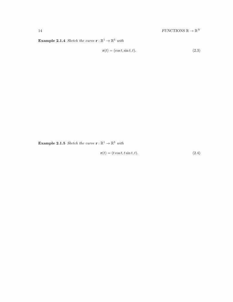
Example 2.1.4 Sketch the curve r : R1 → R3 with
r(t) = (cos t, sin t, t). (2.3)
Example 2.1.5 Sketch the curve r : R1 → R3 with
r(t) = (t cos t, t sin t, t). (2.4)
2.1. CURVES, PATHS AND PARAMETRISATIONS 15
2.1.2 Parameterisations of curves
A parametrisation of a simple curve is defined as follows:
Definition 2.1.6
A parametrisation of a simple curve C of finite length is a path r : [a, b] → C defined on an interval
[a, b] which is one-to-one and onto. If C has infinite length, we can replace the interval [a, b] by
the infinite intervals [a,∞), (∞, b] or (∞,∞) as appropriate. If C is a simple closed curve, we
require r to be one-to-one except at the end points when r(a) = r(b).
Thus a parametrisation of a curve C gives it a coordinate — that is a real number t ∈ R1 which
specifies a unique point on C, and every point of C can be thus specified.
As with paths, it is important to understand that giving a parametrisation of a curve involves
making a choice: There are infinitely different parametrisations for any given curve C — or,
equivalently, infinitely many different ways of giving a coordinate to the curve.
Notes
So why do we need paths and parametrisations?
We need parametrisations to be able to compute derivatives, integrals, lengths, and any other
numerical quantities. The results, such as lengths, will be independent of the particular parametri-
sation used, but we need a parametrisation to be able to compute these.
For example, as we will see, the integral of a function along any curve can be defined as an
abstract mathematical object, but it is impossible to compute in general. To compute it we choose
a parametrisation, and use the Fundamental Theorem of Calculus. Changing the parametrisation
will change the computation, but the answer will always be the same.
16 FUNCTIONS R → RN
Example 2.1.7 Which of the paths in the previous section are parametrisations?
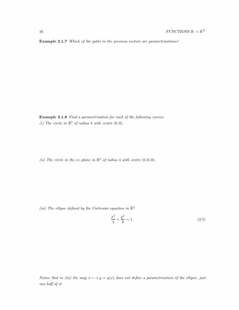
Example 2.1.8 Find a parametrisation for each of the following curves:
(i) The circle in R2 of radius 4 with centre (0, 0).
(ii) The circle in the xz-plane in R3 of radius 4 with centre (0, 0, 0).
(iii) The ellipse defined by the Cartesian equation in R2
x2
4+y2
9= 1 . (2.5)
Notice that in (iii) the map x 7−→ y = y(x) does not define a parametrisation of the ellipse, just
one half of it.
2.1. CURVES, PATHS AND PARAMETRISATIONS 17
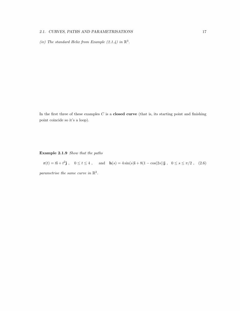
(iv) The standard Helix from Example (2.1.4) in R3.
In the first three of these examples C is a closed curve (that is, its starting point and finishing
point coincide so it’s a loop).
Example 2.1.9 Show that the paths
r(t) = ti+ t2j , 0 ≤ t ≤ 4 , and h(s) = 4 sin(s)i+ 8(1− cos(2s))j , 0 ≤ s ≤ π/2 , (2.6)
parametrise the same curve in R2.
18 FUNCTIONS R → RN
Exercises
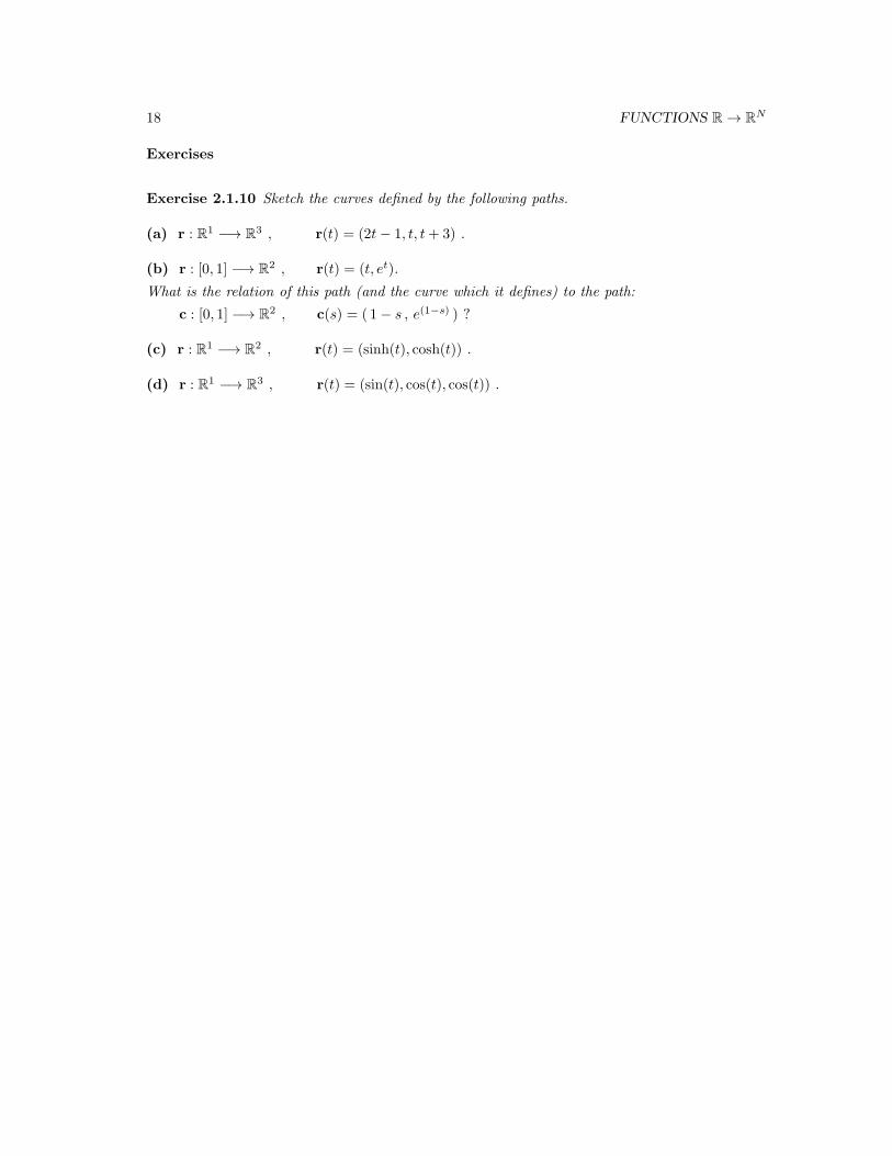
Exercise 2.1.10 Sketch the curves defined by the following paths.
(a) r : R1 −→ R3 , r(t) = (2t− 1, t, t+ 3) .
(b) r : [0, 1] −→ R2 , r(t) = (t, et).
What is the relation of this path (and the curve which it defines) to the path:
c : [0, 1] −→ R2 , c(s) = ( 1− s , e(1−s) ) ?
(c) r : R1 −→ R2 , r(t) = (sinh(t), cosh(t)) .
(d) r : R1 −→ R3 , r(t) = (sin(t), cos(t), cos(t)) .

2.2. DIFFERENTIATION OF PATHS 19
2.2 Differentiation of paths
Before we discuss the generalization, it is worth taking a moment to recall what is meant by the
derivative of a (differentiable) function f : R1 → R1 .
Definition 2.2.1
The derivative f ′(x) exists and is given by the following limit if and only if the limit exists
f ′(x) = limh→0
f(x+ h)− f(x)
h(2.7)
We can rewrite this in a way that will be useful later by introducing the notation o(h) which means
o(h) : a function F of h which satisfies limh→0
F (h)
h= 0 (2.8)
As an example, we can write h sin(h) = o(h) which means
h sin(h) is a function which satisfies limh→0
(h sin(h))/h = 0”. (2.9)
Likewise h2 = o(h), h3 = o(h) but h 6= o(h), sin(h) 6= o(h). Using this notation we have an
equivalent definition of the derivative:
Definition 2.2.2
The derivative f ′(x) exists if and only if the following is true:
f(x+ h) = f(x) + hf ′(x) + o(h) (2.10)
We will use generalisations of this in section 2.4 to write Taylor’s theorem and in section 3.5 to
define the gradient of a function. For the moment we can just use definition 2.2.1 to define the
derivative of a path.
Definition 2.2.3 Given a path (or vector-valued function) r(t) : R → Rn, the derivative of r with
respect to t is defined to be
r′(t) = limh→0
r(t+ h)− r(t)
h. (2.11)
This corresponds to differentiating each vector components of r. For example,
if r(t) =
(
x(t)
y(t)
)
then r′(t) =
(
x′(t)
y′(t)
)
(2.12)
Notice that this coincides with usual derivative of a scalar function when n = 1.
We can also write this out in components using basis vectors i, j, k etc. For a path in R2, if
r(t) = r1(t)i+ r2(t)j then r′(t) = r′1(t)i + r′2(t)j . (2.13)
Similarly, in R3 if
r(t) = r1(t)i+ r2(t)j+ r3(t)k then r′(t) = r′1(t)i + r′2(t)j + r′3(t)k . (2.14)
20 FUNCTIONS R → RN
Examples
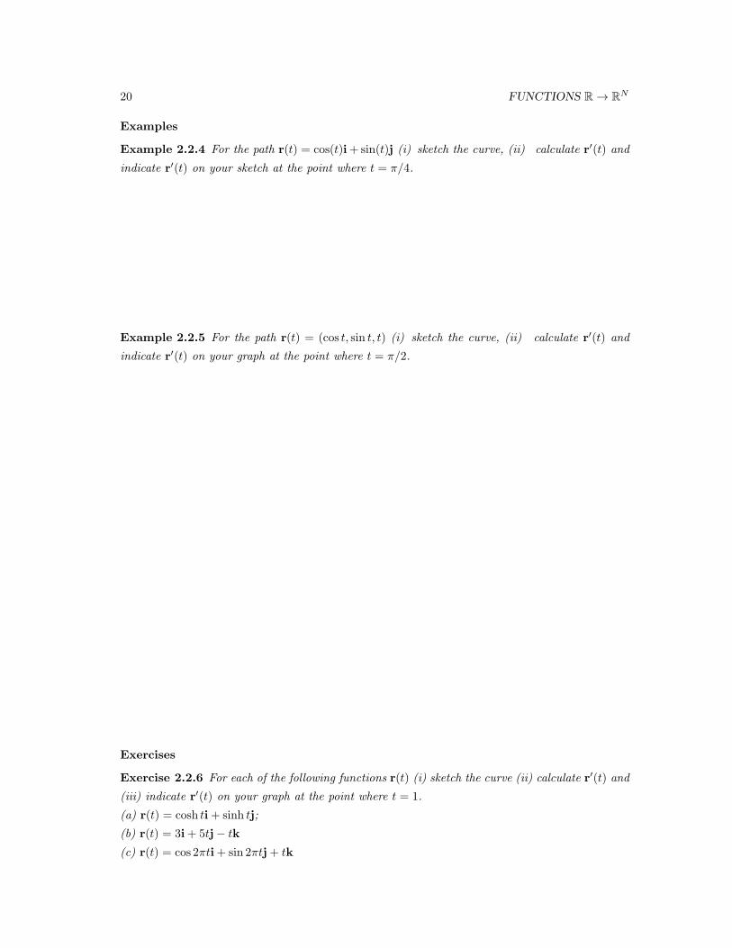
Example 2.2.4 For the path r(t) = cos(t)i+ sin(t)j (i) sketch the curve, (ii) calculate r′(t) and
indicate r′(t) on your sketch at the point where t = π/4.
Example 2.2.5 For the path r(t) = (cos t, sin t, t) (i) sketch the curve, (ii) calculate r′(t) and
indicate r′(t) on your graph at the point where t = π/2.
Exercises
Exercise 2.2.6 For each of the following functions r(t) (i) sketch the curve (ii) calculate r′(t) and
(iii) indicate r′(t) on your graph at the point where t = 1.
(a) r(t) = cosh ti+ sinh tj;
(b) r(t) = 3i+ 5tj− tk
(c) r(t) = cos 2πti+ sin 2πtj+ tk
2.3. TANGENT LINES 21
2.3 Tangent Lines
In some cases, the derivative of a vector function has physical significance; for instance if r(t) is
the position vector of a moving point (with t measuring time) then r′(t) is the velocity of the point
at time t, notice that this is a vector.
This must not be confused with the speed of the particle as it moves along C which is the scalar
function v(t) given by the length of the derivative r′(t), v : R1 −→ R1, t 7−→ ‖r′(t)‖ .
In components, if r(t) = x(t)i + y(t)j+ z(t)k then
r′(t) = x′(t)i+ y′(t)j+ z′(t)k and ||r′(t)|| =√
x′(t)2 + y′(t)2 + z′(t)2 (2.15)
The derivative of a path also has a geometrical meaning. Let C be a simple curve traced out by
the path r(t) as t varies and let p ∈ C be a point on the curve. Then, since C is ‘simple’, there is
a unique t0 ∈ R1 such that p = r(t0). Geometrically r′(t0) := r′(t)|t=t0 is a tangent vector to C
at the point p = r(t0).
But notice, if we change the parametrisation of C, that is, if we choose a different function c(t)
which also traces out the curve C,then just as before, there is unique t1 ∈ R1 such that p = c(t1),
and c′(t1) is a tangent vector to C at the point p = r(t0). But this need not be the same tangent
vector as r′(t0) – the two paths need not have the same velocity.
What will be true is that all the tangent vectors to a curve at a particular point lie on the same
line: there is whole line of tangents; a copy of R1 which touches C ’tangentially’ only at p. If C
is smooth at p, then the tangent line TpC to C is, by definition, the space of all tangent
vectors to the curve at p. This coincides with the geometric idea of a tangent line.
If C is smooth at p ∈ C, and we choose a parametrisation r : R1 −→ C ⊂ Rn of C, we can use r′(t)
to write down an explicit equation for the tangent line to the curve at the point p: The tangent
line can be parametrised as
l(µ) = r(t0) + µr′(t0) (2.16)
Note that changing the parametrisation may change the equation of the tangent line but it always
defines the same line of course.
Recall, that the ‘length’, or ‘norm’, ‖a‖ of a vector a = (a, b, c) ∈ R3 is defined by
‖a‖ =√a2 + b2 + c2 .
Important Task: Revise the ideas of the scalar (or dot) product for vectors in R2 or R3, and
how one uses this to compute length of vectors, the angle between two vectors in appendix A.
Revise also the vector product of two vectors, and how this is used to compute the area of the
parallelogram defined by two vectors.
22 FUNCTIONS R → RN
Examples
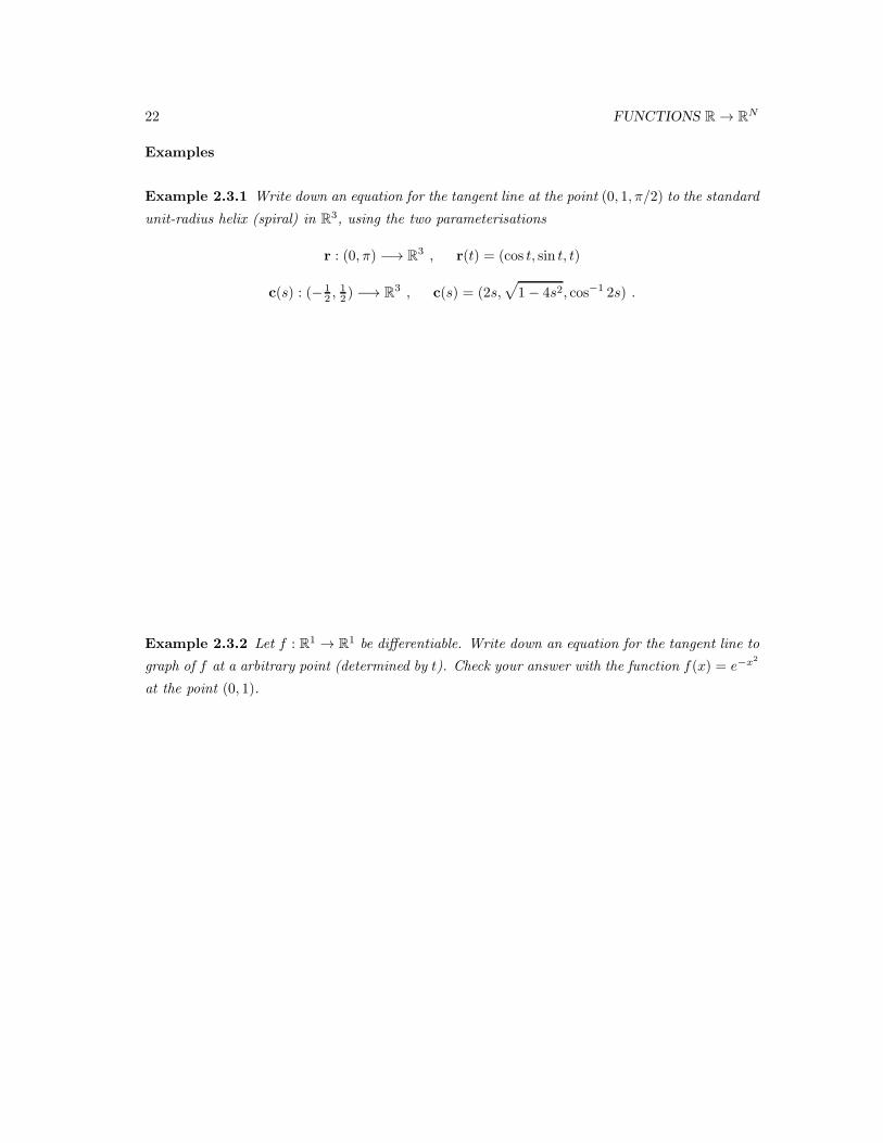
Example 2.3.1 Write down an equation for the tangent line at the point (0, 1, π/2) to the standard
unit-radius helix (spiral) in R3, using the two parameterisations
r : (0, π) −→ R3 , r(t) = (cos t, sin t, t)
c(s) : (− 12 ,
12 ) −→ R
3 , c(s) = (2s,√
1− 4s2, cos−1 2s) .
Example 2.3.2 Let f : R1 → R1 be differentiable. Write down an equation for the tangent line to
graph of f at a arbitrary point (determined by t). Check your answer with the function f(x) = e−x2
at the point (0, 1).
2.3. TANGENT LINES 23
Exercises
Exercise 2.3.3 Sketch the curves defined by the following paths.
(a) r : [−π4 ,
π4 ] −→ R2 , r(t) = (t, tan(t)).
How does this path (and the curve which it defines) compare to the path:
c : [0, π2 ] −→ R2 , c(s) = (π/4− s , tan(π/4− s) ) ?
(b) r : R1 −→ R3 , r(t) = ( sin(t) , 5 cos(t) , cos(2t) ) .
Exercise 2.3.4 Compute r′(0) for each of the paths in exercise 2.3.3. Hence compute, in each
case, a parametric equation of the tangent line to the curve at r(0).
Exercise 2.3.5 Suppose that a = a1i+ a2j+ a3k is a constant vector. Show that ddta = 0.
24 FUNCTIONS R → RN
2.4 Taylor’s Theorem for Vector-valued Functions
We can understand the derivative r′(t0) as the first term in the Taylor expansion of r(t) around
t = t0. Taylor’s Theorem tells us that provided the derivatives
r(k)(t) =dk
dtkr(t)
in R3
= (x(k)(t), y(k)(t), z(k)(t))
all exist, then we can approximate the, possibly very complicated, curve C traced out by r(t) using
simple polynomials; straight lines, parabolae, cubics, quartics, . . . .
The Taylor expansion to first order (2.10) generalized to paths, i.e. vector-valued functions is:
r(t+ h) = r(t) + h r′(t) + o(h) , (2.17)
where o(h) is a vector such that o(h)/h→ 0 as h→ 0.
The first two terms in (2.17), precisely gives the equation of the tangent line at r(t):
l(h) = r(t) + h r′(t)
The tangent line corresponds to the linear approximation to the value of r(t + h) that we can
compute by knowing r(t) and its derivative.
We can generalize this, and obtain the Taylor expansion to second order
r(t+ h) = r(t) + h r′(t) +h2
2r′′(t) + o(h2) . (2.18)
Here, o(h2) is a vector such that o(h2)/h2 → 0 as h→ 0, while
r′′(t) :=d2
dt2r(t) =
x′′(t)
y′′(t)
z′′(t)
,
where x : R1 → R1, y : R1 → R1, z : R1 → R1 are the scalar-functions which are the components
of r(t).
This gives us a quadratic approximation (in h) around r(t) ∈ C to the actual curve C, which will
be a better approximation than the linear approximation (2.17) obtained from computing just the
first-derivative.
2.4. TAYLOR’S THEOREM FOR VECTOR-VALUED FUNCTIONS 25
Examples
Example 2.4.1 Compute the first-order and second-order Taylor expansions around the point
(0, 1) to the path
r : R −→ R2 , r(t) = (t, e−t2)
interpreting the result geometrically.
Example 2.4.2 Prove Equation (2.17) using the result Equation (2.10) for scalar functions in the
case of R2
26 FUNCTIONS R → RN
2.5 Product rules for differentiation of paths
There are product rules and chain rules for vector functions. (Chain rules are considered later,
in section 4.1.) Since there are three kinds of products (product of a vector by a scalar, scalar
product of two vectors, vector product of two vectors) there are three product rules – but they are
all very similar.
Theorem 2.5.1 Suppose that r(t) is a vector-valued function and λ(t) : R → R is a scalar func-
tion. Thend (λ(t)r(t))
dt= λ′(t)r(t) + λ(t)r′(t) (2.19)
Proof: we can write the path out in components and use the product rule to differentiate each
component separately
Examples
Example 2.5.2 Differentiate the function r(t) = t2(5ti+ sin tj)
Example 2.5.3 Suppose that a and b are constant vectors. Differentiate the function r(t) =
et(a+ 3b).
In both examples we could, of course, have obtained the same result by expanding out the product
and then differentiating.
Exercises
Exercise 2.5.4 (a) Differentiate r(t) = (cos t)(ti+ 5j) with respect to t.
(b) Differentiate r(t) = 3t2a+ cos tb with respect to t, given that a and b are constant vectors.
2.5. PRODUCT RULES FOR DIFFERENTIATION OF PATHS 27
Theorem 2.5.5 Suppose that g(t) and r(t) are vector-valued functions. Then
d (r(t) · g(t))dt
= r′(t) · g(t) + r(t) · g′(t) (2.20)
Proof:
we can use Taylor’s theorem Equation (2.17) and substitute this into the definition of the derivative,
Equation (2.7):
The following result, relating the derivative of a vector and the derivative of its length, is often
useful.
Proposition 2.5.6 Suppose that r(t) is a vector function and n(t) = |r(t)| the scalar function
defined by the norm of r(t). Then
n(t)n′(t) = r(t) · r′(t). (2.21)
Proof: we can differentiate both sides of the equality r · r = n2.
28 FUNCTIONS R → RN
Corollary 2.5.7 Suppose that r(t) is a vector of constant (non-zero) length. Then r′(t) is per-
pendicular to r(t). In other words, if n = const then r ·r′ = 0. Provided r(t) 6= 0 then the converse
holds
Proof:
Proof of the converse: If r is perpendicular to r′ then r · r′ = 0 ⇒ nn′ = 0 and so either n = 0 (a
constant) or n′ = 0 in which case n is a constant. In either case, n is a constant.
Examples
Example 2.5.8 Show that the vector r(t) = 3 cos ti+ 3 sin tj has constant length.
Exercises
Exercise 2.5.9 Find r′(t) for each of the following functions:
(a) r(t) = (i + tj) · (3ti+ 4j);
(b) r(t) = (a+ tb) · (c + tb);
Exercise 2.5.10 Suppose that a and b are perpendicular and of equal length. Show that
d ((a + tb) · (ta+ tb))
dt= 0 when t = − 1
2 . (2.22)
If a is a vector then a or |a| is used to denote the length of a. It is important to remember that
a = |a| = √a · a.
Exercise 2.5.11 Find the time t (with 0 < t < π/2) at which the length of the vector r(t) =√2 sin ti+ cos 2tj is a minimum.
2.5. PRODUCT RULES FOR DIFFERENTIATION OF PATHS 29
The third product theorem concerns vector products. Because the vector product is not commu-
tative it is essential to write the factors in the correct order.
Theorem 2.5.12 Suppose that r(t) and g(t) are vector-valued functions. Then
d (r(t)× g(t))
dt= r′(t)× g(t) + r(t)× g′(t) (2.23)
Proof: Exercise below
Examples
Example 2.5.13 Find the derivative of r(t) = (a + tb) × (b + ta), where a and b are constant
vectors.
SUMMARY
Let r,g : R1 → Rn be vector valued functions, and λ : R1 → R1 a scalar function.
d (r(t) + g(t))
dt= r′(t) + g′(t) (2.24)
d (λ(t)r(t))
dt= λ′(t)r(t) + λ(t)r′(t) (2.25)
d (r(t) · g(t))dt
= r′(t) · g(t) + r(t) · g′(t) (2.26)
d (r(t)× g(t))
dt= r′(t)× g(t) + r(t)× g′(t) (2.27)
30 FUNCTIONS R → RN
Exercises
Exercise 2.5.14 Prove Theorem (2.5.12)
Exercise 2.5.15 Find r′(t) for each of the following functions:
(a) r(t) = (3ti+ 2t2j+ k) × (4t3i+ j+ tk);
(b) r(t) = eta× (a+ tb);
Exercise 2.5.16 Show thatd (r(t)× r′(t))
dt= r(t) × r′′(t).
Exercise 2.5.17 Suppose that r(t), g(t) and h(t) are vector functions. Find an expression for the
derivative (with respect to t) of the scalar triple product (r(t)×g(t))·h(t) in terms of r(t),g(t),h(t), r′(t),g′(t)
and h′(t).
31
Chapter 3
Functions Rm → R
In this chapter we will study derivatives of scalar functions of several variables, that is functions
f : Rm → R .
We start with functions of two variables and for these we can gain many insights by considering the
functions as defining a surface in R3. This surface can be thought of as the graph of the function
in a way we make clear in the next section.
3.1 Graphs of scalar functions
Definition 3.1.1 The graph of f : Rm → R1 is the m-dimensional subset of Rm+1 defined by
Graph(f) = (x , f(x) ) ∈ Rm+1 | x ∈ R
m . (3.1)
In components, we can write
(x , f(x) ) = (x1, x2, . . . , xm, f(x1, x2, . . . , xm))
For example, if f : R2 → R, f(x, y) = x2 − y2 then
Graph(f) = (x, y, x2 − y2) | (x, y) ∈ R2 ⊂ R
3 (3.2)
Thus, the case of f : R1 → R1 this coincides with our usual idea of the graph: If f : R → R, then
Graph(f) = (x, f(x)|x ∈ R = set of points with y = f(x).
32 FUNCTIONS RM → R
It is important for us to be able to get a good geometric understanding of the graph of scalar
functions and to be able to sketch them. For f : R2 → R the graph is a two-dimensional subset of
R3, for f : R3 → R the graph is three-dimensional subset of R4! A useful too for scalar functions
in higher dimensions is to look at ”snapshots” or slices of the graph.
Horizontal Slices
One of the means which may be used to deduce the shape of the graph of a function of one variable
is to look at a horizontal slice, or level set at height c: this just means the subset of R1
Sy=c = x ∈ R1 | f(x) = c (3.3)
Equivalently Sy=c is the intersection of the graph of f and the horizontal line y = c, that is the
points of Graph(f) at height c above the x–axis.
For example, for f = x2, the slice Sy=2 = x|x2 = 2 = −√2,√2 consists of two points.
We can try applying the same idea in the next dimension up when looking how to sketch the graph
of a function f : R2 → R1.
For such a function three axes, labelled x, y and z, are needed. The graph z = f(x, y) then
represents the function and looks like a curved 2-dimensional subset (a surface) of 3-space
Graph(f) = (x, y, f(x, y)) ∈ R3 | (x, y) ∈ R
2 ⊂ R3 .
Notice that the z-coordinate z = f(x, y) tells us the height of the surface above the xy–plane.
3.1. GRAPHS OF SCALAR FUNCTIONS 33
This is useful when we come to sketch the graph. Indeed, we can again look at a horizontal slice,
or level ‘curve’ at height c: this just means the 1-dimensional subset of R2
Sz=c = (x, y) ∈ R2 | f(x, y) = c (3.4)
Equivalently,
Sz=c = Graph(f) ∩ (the plane z = c)
is the curve obtained by intersecting the graph of f with the horizontal plane z = c.
In fact, one way think of a surface (arising here as a graph) is as a union of curves: a sphere is a
collection of circles and a the hyperbolic paraboloid z = x2−y2 is a collection of hyperbolae stacked
vertically
Vertial slices
We can also take vertical slices: this means the intersection of the graph of f with a vertical
plane: for example x = c a constant:
Svertx=c = (y, z) ∈ R
2 | f(c, y) = z (3.5)
or for y = c a constant
Sverty=c = (x, z) ∈ R
2 | f(x, c) = z (3.6)
In this way we build up a picture of what the graph of f looks like ‘frame by frame’. In this case
the hyperbolic paraboloid z = x2 − y2 is a collection of parabolae when sliced vertically:
34 FUNCTIONS RM → R
Examples
Example 3.1.2 Sketch the graph z = f(x, y) for the functions f : R2 → R1 with
(a) f(x, y) = x2 − y2 .
(b) f(x, y) = x2 + y2 .
Note that apparently similar functions can, in fact, lead to dramatically different surfaces
Notice that the use of polar coordinates made sketching the surfaces easier here: we will be often
use different coordinate systems as we go along.
3.1. GRAPHS OF SCALAR FUNCTIONS 35
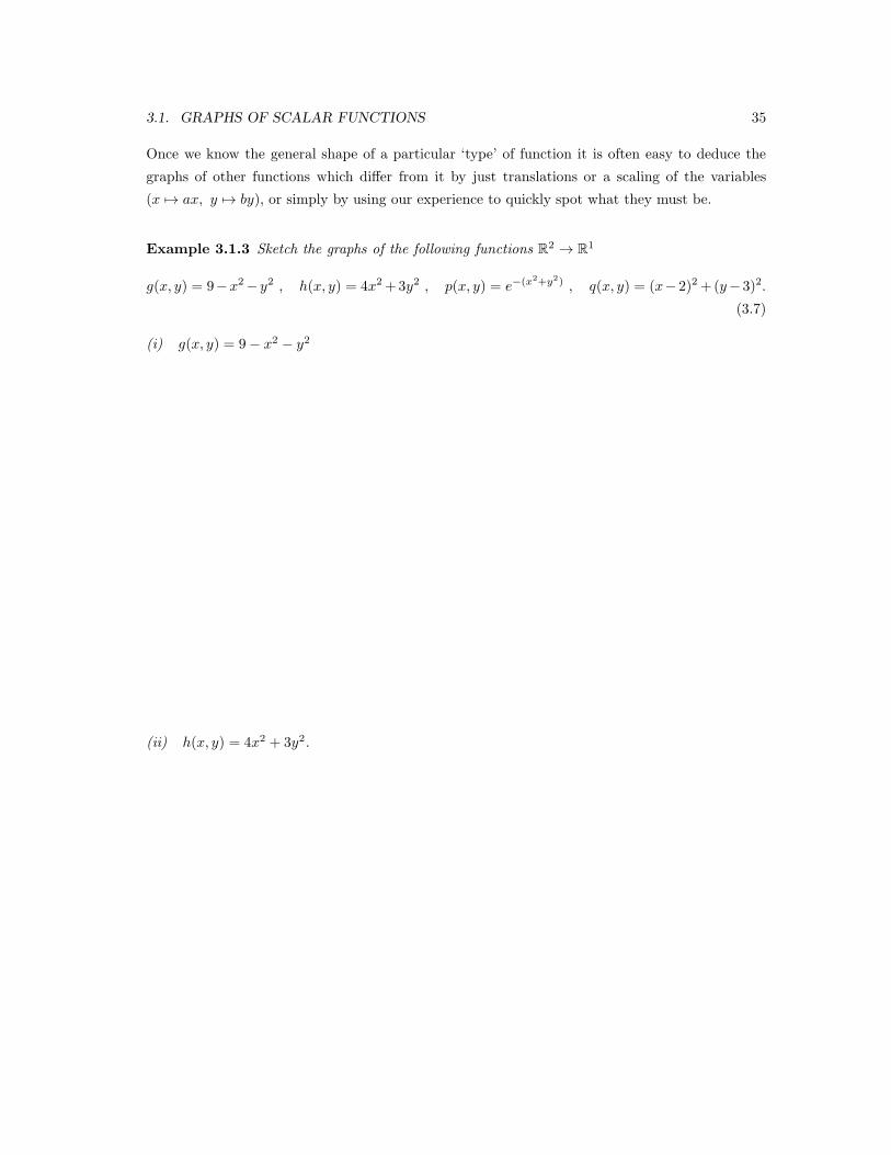
Once we know the general shape of a particular ‘type’ of function it is often easy to deduce the
graphs of other functions which differ from it by just translations or a scaling of the variables
(x 7→ ax, y 7→ by), or simply by using our experience to quickly spot what they must be.
Example 3.1.3 Sketch the graphs of the following functions R2 → R1
g(x, y) = 9−x2− y2 , h(x, y) = 4x2+3y2 , p(x, y) = e−(x2+y2) , q(x, y) = (x− 2)2+(y− 3)2.
(3.7)
(i) g(x, y) = 9− x2 − y2
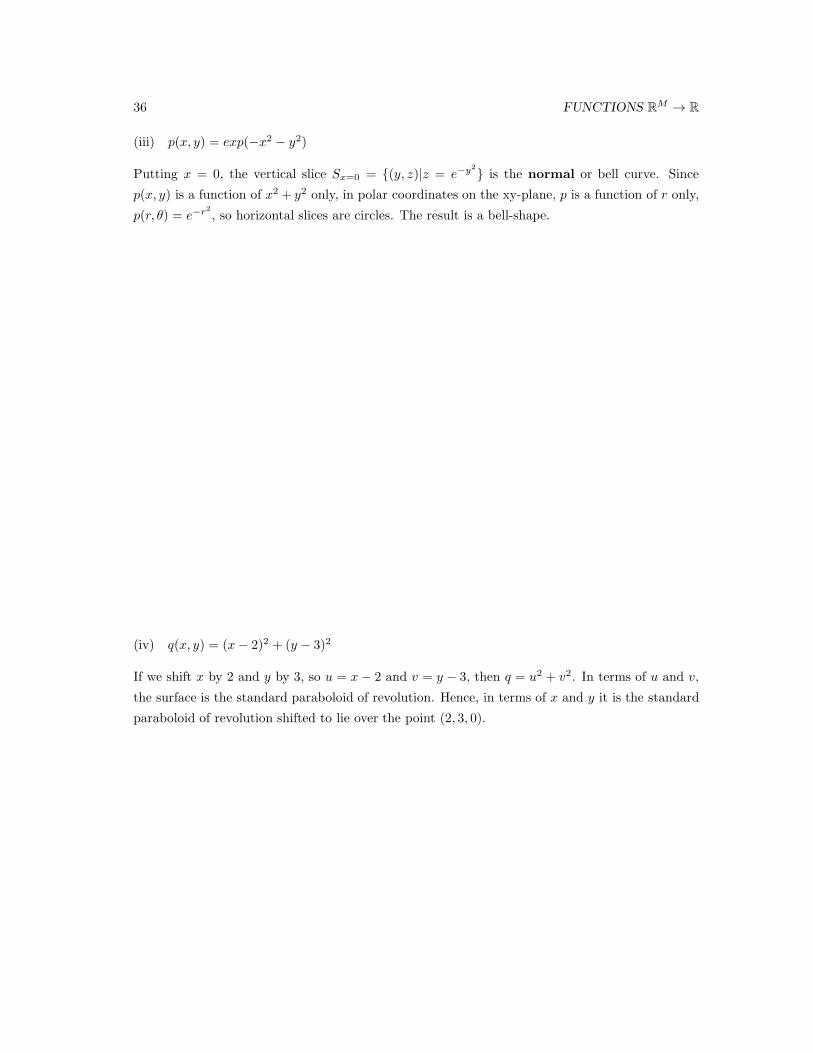
(ii) h(x, y) = 4x2 + 3y2.
36 FUNCTIONS RM → R
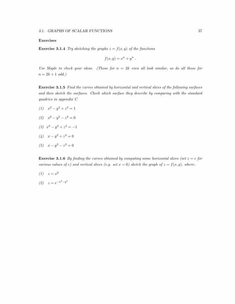
(iii) p(x, y) = exp(−x2 − y2)
Putting x = 0, the vertical slice Sx=0 = (y, z)|z = e−y2 is the normal or bell curve. Since
p(x, y) is a function of x2 + y2 only, in polar coordinates on the xy-plane, p is a function of r only,
p(r, θ) = e−r2, so horizontal slices are circles. The result is a bell-shape.
(iv) q(x, y) = (x− 2)2 + (y − 3)2
If we shift x by 2 and y by 3, so u = x− 2 and v = y − 3, then q = u2 + v2. In terms of u and v,
the surface is the standard paraboloid of revolution. Hence, in terms of x and y it is the standard
paraboloid of revolution shifted to lie over the point (2, 3, 0).
3.1. GRAPHS OF SCALAR FUNCTIONS 37
Exercises
Exercise 3.1.4 Try sketching the graphs z = f(x, y) of the functions
f(x, y) = xn + yn .
Use Maple to check your ideas. (Those for n = 2k even all look similar, as do all those for
n = 2k + 1 odd.)
Exercise 3.1.5 Find the curves obtained by horizontal and vertical slices of the following surfaces
and then sketch the surfaces. Check which surface they describe by comparing with the standard
quadrics in appendix C
(1) x2 − y2 + z2 = 1
(2) x2 − y2 − z2 = 0
(3) x2 − y2 + z2 = −1
(4) x− y2 + z2 = 0
(5) x− y2 − z2 = 0
Exercise 3.1.6 By finding the curves obtained by computing some horizontal slices (set z = c for
various values of c) and vertical slices (e.g. set x = 0) sketch the graph of z = f(x, y), where:
(1) z = x2
(2) z = e−x2−y2
38 FUNCTIONS RM → R
3.2 Directional derivatives
Using our knowledge of how to differentiate paths, we now study derivatives of scalar-valued
functions in two and three dimensions. We do this by constructing curves in the graph of the
function. A curve in R2 gives a curve in the surface in R3 which is the graph of f . The simplest
curves in R2 are straight lines and these lead to the idea of directional derivatives.
Suppose we have a scalar function
f : Rm −→ R1
(m = 1, 2, 3). Suppose we choose a fixed unit vector u ∈ Rm. This defines a direction, and one
can look at the rate of change of a function f(x) corresponding to changes in x in the direction of
u. This leads to the definition of the directional derivative:
Definition 3.2.1 If u is a fixed unit vector, the directional derivative f ′u(x) of the function f(x)
in the direction u is defined to be
f ′u(x) = lim
h→0
f(x+ hu)− f(x)
h. (3.8)
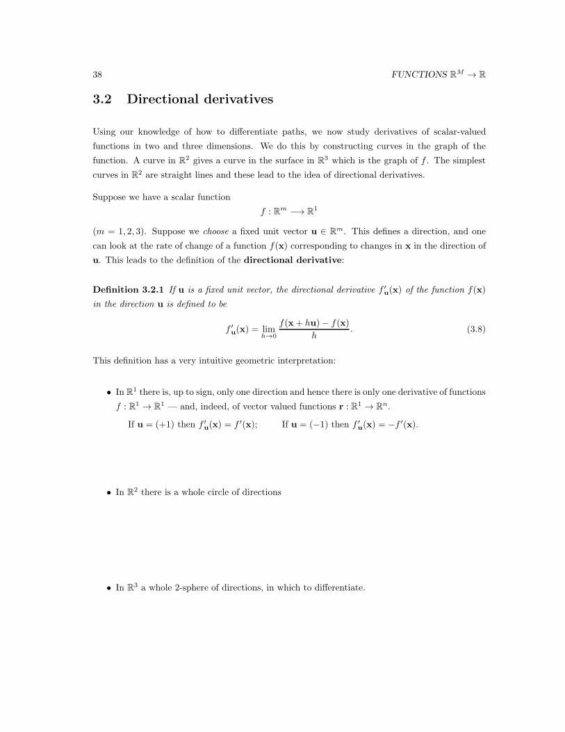
This definition has a very intuitive geometric interpretation:
• In R1 there is, up to sign, only one direction and hence there is only one derivative of functions
f : R1 → R1 — and, indeed, of vector valued functions r : R1 → Rn.
If u = (+1) then f ′u(x) = f ′(x); If u = (−1) then f ′
u(x) = −f ′(x).
• In R2 there is a whole circle of directions
• In R3 a whole 2-sphere of directions, in which to differentiate.
3.2. DIRECTIONAL DERIVATIVES 39
Hence in two and three dimensions we have to say in which direction we are going to differentiate.
Once we have chosen a direction u ∈ Rm, this defines the path r(t) = x+tu in Rm passing through
x = r(0) in the direction u.
This in turn defines a path in the surface Graph(f),
r(t) = (r(t), f(r(t))) = (x + tu, f(x+ tu))
The last component of r(t), f(r(t)) = f r(t), is clearly a scalar function R → R which can be
differentiated in the usual sense of a 1-variable scalar function (‘Calculus I’). We have the important
identity
Lemma 3.2.2 The directional derivative of a scalar function f : Rm → R in the direction u is
f ′u(x) =
d
dt
∣∣∣∣t=0
f(x+ tu) (3.9)
Proof:d
dt
∣∣∣∣t=0
f(x+ tu) = limh→0
f(x+ (t+ h)u)− f(x+ tu)
h
∣∣∣∣t=0
= limh→0
f(x+ hu)− f(x)
h= f ′
u(x)
from Definition (3.2.1).
Note: the directional derivative of f : Rm → R1 is always a scalar function f ′u: Rm → R1, that is,
at each point of x ∈ Rm it defines a number, not a vector.
Geometrically, the derivative of the path r(t) gives us a tangent vector to the surface Graph(f).
The derivative r′(0) is a tangent vector at the point r(0). We can find this tangent vector explicitly:
r : R → Graph(f) , t 7→ (r(t), f(r(t))) = (x + tu, f(x+ tu))
so the vector
r′(0) = (u,d
dtf(x+ tu)
∣∣∣∣t=0
) = (u , f ′u(x) ) (3.10)
is tangent to the curve C in the graph of F and hence is tangent to the whole surface.
40 FUNCTIONS RM → R
Examples
Example 3.2.3 Calculate f ′u(x) if u = 1
3 (i+2j+2k) and f(x) = x2 + yz by direct application of
Definition (3.2.1) and using Equation (3.9)
First, we note that |u|2 = 19 (1 + 4 + 4) = 1 and so u is a unit vector.
Now to use Definition (3.2.1):
f ′u(x) = lim
h→0
f(x+ hu)− f(x)
h= lim
h→0
((x+ h/3)2 + (y + 2h/3)(z + 2h/3)− x2 − yz
h
)
= limh→0
(2x
3+
2y
3+
2z
3+
5
9h
)
=2
3(x+ y + z) (3.11)
Now using Equation (3.9):
f ′u(x) =
d
dtf(x+ tu)
∣∣∣∣t=0
=d
dt
((x+ t/3)2 + (y + 2/3t)(z + 2/3t)
)∣∣∣∣t=0
=2
3(x+ y + z) (3.12)
Example 3.2.4 Compute all tangent vectors to the standard elliptic paraboloid (i.e. the graph of
z = x2 + y2) at the point (1, 1, 2).
Firstly, (1, 1, 2) is the point (1, 1, f(1, 1)) so we need to consider directions u = (cos(θ), sin(θ)) and
paths x+ tu = (1 + t cos(θ), 1 + t sin(θ)).
f(x+ tu) = 1 + 2t(cos(θ) + sin(θ)) + t2 ⇒ d
dtf(x+ tu)
∣∣∣∣t=0
= 2(cos(θ) + sin(θ))
So, the tangent vectors we obtain are
(u, f ′u(x)) =
cos(θ)
sin(θ)
2 cos(θ) + 2 sin(θ)
= cos(θ)
1
0
2
+ sin(θ)
0
1
2
. (3.13)
3.2. DIRECTIONAL DERIVATIVES 41
Definition 3.2.5 Let S be a surface in R3, and suppose that S is smooth enough near p ∈ S. A
tangent vector to S at p is the derivative (vector) evaluated at p ∈ S of a path which lies in S
and passes through p.
In example Example (3.2.4) the tangent vectors all lie in the plane spanned by (1, 0, 2) and (0, 1, 2).
This is true more generally, the tangent vectors to a surface at point (usually) span a plane called
the Tangent Plane which is defined as follows.
Definition 3.2.6 Let S be a surface in R3, and suppose that S is smooth enough near p ∈ S. The
tangent plane (or just tangent space) to S at p is the 2-dimensional plane in R3 which is spanned
by all tangent vectors to S at p.
NB: “Smooth enough near p ∈ S” just means that all such derivatives exist.
We can find the equation of this tangent plane as follows:
• Recall the plane through a with normal n is the set of points x satisfying (x−a) · n = 0.
• Secondly, if v and w are two non-zero non-parallel vectors in a plane then n = v ×w is a
non-zero normal to that plane
• We can find two non-zero non-parallel vector in the tangent plane TpS using Equation (3.10)
with the two choices u1 =
(
1
0
)
and u2 =
(
0
1
)
. These define two paths in Graph(f)
c1(t) = (x0 + tu1, f(x0 + tu1)) (3.14)
c2(t) = (x0 + tu2, f(x0 + tu2)) (3.15)
• These in turn give two tangent vectors in TpS
c′1(0) = (u1, f′u1(x0)) =
1
0
f ′u1(x)
c′2(0) = (u2, f′u2(x0)) =
0
1
f ′u2(x)
(3.16)
• These allow us to find a normal n to TpS as
n = c′1(0)× c′2(0) =
−f ′u1(x0)
−f ′u2(x0)
1
(3.17)
• Hence, the equation of the tangent plane TpS at x0 is
(x− x0) · n = 0 or f ′u1(x0)(x− x0) + f ′
u2(x0)(y − y0) = (z − z0) (3.18)
42 FUNCTIONS RM → R
Exercises
Exercise 3.2.7 Use first principles, as in Example (3.2.3), to calculate g′u(x) if
g(x) = x2yz and u = 113 (3i+ 4j+ 12k).
3.3 Partial derivatives
When evaluating directional derivatives it is easier to use a rule than first principles. To write that
down we first need to introduce some other special cases of directional derivatives.
Although we can differentiate in any one of infinitely many different directions in Rm (m = 2, 3),
there are nevertheless the special directions defined by the coordinate axes given by taking u =
ei, i = 1, . . . , n; thus, in
R2 : e1 =
(
1
0
)
= i e2 =
(
0
1
)
= j ,
R3 : e1 =
1
0
0
= i e2 =
0
1
0
= j , e2 =
0
0
1
= k .
These preferred choices of directions give natural generalisations of the derivative in one dimension
and define the so-called partial derivatives of a function f : Rm → R1.
Definition 3.3.1 When it exists, the ith partial derivative ∂f∂xi
of a scalar-valued function
f : Rm → R1 at x ∈ Rm, is defined by
∂f
∂xi
∣∣∣∣x
:= f ′ei(x) (3.19)
(When all the partial derivatives exist and are continuous we say that f is differentiable at x).
Equivalently:∂f
∂xi=
d
dtf(x0 + tei)
∣∣∣∣t=0
. (3.20)
• In R2 we have 2 partial derivatives:
3.3. PARTIAL DERIVATIVES 43
• In R3 we have 3 partial derivatives:
Let g : R3 → R , (x, y, z) 7→ g(x, y, z). Then
∂g
∂x1=
∂g
∂x=
d
dtg(x+ t, y, z)
∣∣∣∣t=0
(diffn w.r.t x while y and z are kept fixed)
∂g
∂x2=
∂g
∂y=
d
dtg(x, y + t, z)
∣∣∣∣t=0
(diffn w.r.t y while x and z are kept fixed)
∂g
∂x3=
∂g
∂z=
d
dtg(x, y, z + t)
∣∣∣∣t=0
(diffn w.r.t z while x and y are kept fixed)
Thus the partial derivative ∂f∂x with respect to x is obtained by differentiating with respect to
the x-variable on its own, treating the y and z variables as constants; likewise, ∂f∂y is obtained by
differentiating with respect to the y-variable on its own, treating the x and z variables as constants
— and so forth.
Examples
Example 3.3.2 Compute the partial derivatives of the functions R2 → R1 defined by
(i) f(x, y) = x2y + cosx
(ii) f(x, y) = ex log y +√xy, (for x, y > 0)
(iii) f(x, y) = e−(x2+y2) .
44 FUNCTIONS RM → R
Example 3.3.3 Compute the partial derivatives of the functions R3 → R1 defined by
(i) g(x, y, z) = x2y2z2 + z cosx
(ii) g(x, y, z) = log(1 + x2y2 + z2) .
3.4. A FORMULA FOR THE TANGENT PLANE TO A SURFACE 45
3.4 A formula for the tangent plane to a surface
Proposition 3.4.1 Let f : R2 −→ R1 be differentiable at (x, y) ∈ R2. The tangent plane to the
graph-surface of f at the point (x0, y0, f(x0, y0)) is given by
z = z0 + (x− x0)
(∂f
∂x
)∣∣∣∣x0
+ (y − y0)
(∂f
∂y
)∣∣∣∣x0
. (3.21)
where the partial derivatives are evaluated at x0 = (x0, y0).
Proof:
Example 3.4.2 Compute the equations of the tangent planes to
(i) the surface z = x2y2 at the point (1, 1, 1),
(ii) the surface z = e−(x2+y2) at the point (0, 0, 1).
46 FUNCTIONS RM → R
3.5 The gradient of a scalar function
We have defined directional derivatives and partial derivatives but it would still be good to define
the derivative of a function of several variables. When we try to adapt the first definition of the
derivative of a scalar function to functions f : Rm −→ R1 with m > 1 we find a problem: We
cannot define “ limh→0
f(x+ h)− f(x)
h” since we cannot divide by a vector.
Instead, we can adapt the second definition to define a gradient vector field which plays the role for
scalar functions of several variables that the usual derivative plays for scalar functions of a single
variable.
Definition 3.5.1 (1) A scalar function f(x) ∈ R1 of a vector variable x ∈ Rm is differentiable
if there exists a vector function ∇f(x) such that
f(x+ h)− f(x) = h · ∇f(x) + (h) , (3.22)
where “(h)” means that the term is so small that even when divided through by |h| the result
still tends to zero as |h| tends to zero.
(2) The vector ∇f(x) is called the gradient of f at x. The map
Rm −→ R
m , x 7−→ ∇f(x)
is called the gradient vector field associated to f .
In particular:
• If f is a scalar function on R2, x 7−→ f(x) = f(x, y) then ∇f is a vector field on R2,
∇f : R2 → R
2 (3.23)
• If g is a scalar function on R3, x 7−→ g(x) = g(x, y, z) , then ∇g is a vector field on R3,
∇g : R3 → R
3 . (3.24)
As with ordinary differentiation, one usually uses rules rather than ‘first principles’ to evaluate a
gradient. The key result is that ∇f can be written very simply in terms of the partial deriviatives
of f :

3.5. THE GRADIENT OF A SCALAR FUNCTION 47
Theorem 3.5.2
If f : R2 −→ R1 has partial derivatives ∂f∂x ,
∂f∂y then in Cartesian (rectangular) coordinates
∇f =∂f
∂xi+
∂f
∂yj =
(∂f∂x∂f∂y
)
(3.25)
Similarly, if f : R3 −→ R1 has partial derivatives ∂f∂x ,
∂f∂y ,
∂f∂z then in Cartesian coordinates
∇f =∂f
∂xi+
∂f
∂yj+
∂f
∂zk =
∂f∂x∂f∂y∂f∂z
(3.26)
Outline proof for the case of R2:
48 FUNCTIONS RM → R
Examples
Example 3.5.3 Calculate ∇f for f : R2 −→ R1 with f(x) = x2 − y2, and, sketch the gradient
vector field and also the contours of constant f .
The following example is important in theoretical physics for describing electric or gravitational
fields:
Example 3.5.4 If r = xi + yj + zk and n = |r| : R3 −→ R1, so n(x) =√
x2 + y2 + z2 , the
length of the vector r, show that
∇(n) =r
n(3.27)
∇(1
n
)
= − r
n3. (3.28)
These examples suggest the result
∇(nk) = knk−2r. (3.29)
3.5. THE GRADIENT OF A SCALAR FUNCTION 49
Exercises
Exercise 3.5.5 Use the definition to evaluate ∇f if f(x) = xy + zx.
[Solution: ∇f = (y + z)i+ xj+ xk]
Exercise 3.5.6 Compute ∇f where f(x, y, z) = x2 + y2 + z2. Use this to show that the formula
(3.29) is true for n = 2.
Exercise 3.5.7 Prove the formula (3.29).
Exercise 3.5.8 Calculate the gradient of each of the following functions: (a) f(x) = (xy)/z, (b)
f(x) = sin(x + y + z), (c) f(x) = xyez.
50 FUNCTIONS RM → R
3.5.1 Alternative formula for the tangent plane to a surface
Let f : R2 −→ R1 be differentiable at (x, y) ∈ R2. Then the equation for the tangent plane (3.21)
at the point (x0, y0, z0 = f(x0, y0)) can be rewritten using the gradient of f as follows:
z = z0 + (x− x0) · ∇f(x0) (3.30)
3.6. THE RATE OF CHANGE OF A FUNCTION F : RM −→ R1 51
3.6 The rate of change of a function f : Rm −→ R1
We can also use the gradient vector field to deduce a simple formula for calculating any directional
derivative:
Theorem 3.6.1 Suppose that f : Rm −→ R1 is differentiable and suppose that u ∈ Rm is a unit
vector. Then
f ′u(x) = u · ∇f(x) (3.31)
NB Notation for f ′u varies. You may find Duf(x), Luf(x) or simply u · ∇f used as alternatives.
By definition, the directional derivative of a function f : Rm → R1 in the direction u ∈ R3 tells us
The rate of change of the value of the function f in the direction u.
In particular – using directional derivatives it is easy to see in which direction a function is changing
most, or least. First note that f ′u(x) is the component of ∇f(x) in the direction of u.
Thus at a point x ∈ Rm the value f(x) ∈ R of the function f : Rm −→ R increases most
rapidly in the direction of ∇f(x) ∈ Rm and decreases most rapidly in the direction of
−∇f(x) ∈ Rm.
52 FUNCTIONS RM → R
Examples
Example 3.6.2 Show that the derivative of f(x) = x3 + sin(y + z) in the direction of i+ j+ k is1√3 (3x
2 + 2 cos(y + z)).
Example 3.6.3 Find the direction in which the function f(x) =√
1− (x2 + y2) is increasing
most rapidly. Sketch the vector field ∇f and the contours of constant f . (A two dimensional
example is used, because it can be visualised.)
In two examples, Example (3.5.3) and Example (3.6.3) we have seen here that the gradient vector
field is orthogonal to the level sets of a function f : Rn −→ R1,. This is a general results and the
next two sections will enable us to explain why.
Exercises
Exercise 3.6.4 Use the result Equation (3.31) to check your answer to Exercise (3.2.7).
Exercise 3.6.5 Calculate f ′u(x) when u = (i + j)/
√2 and f(x) = 3x/(x− y).
Exercise 3.6.6 Find the derivative of f(x) = x/y at the point P = (1, 3, 5) in the direction of
~PQ if Q is the point (2, 4, 8). [Answer 2/(9√11)]
Exercise 3.6.7 If a is a constant vector, show that the directional derivative of f(x) = a · x in
the direction of a is equal to |a|.Exercise 3.6.8 Find the direction in which f(x) = x2 + y2− 4z2 is increasing most rapidly at the
point (1, 1, 1). Also find this rate of increase. [Answer 6√2]
Exercise 3.6.9 Find the direction in which f(x) = xz2y3 is increasing most rapidly at the point
(1, 2,−1). Also find this rate of increase. [Answer 4√29]
3.7. TAYLOR’S THEOREM IN TWO VARIABLES 53
3.7 Taylor’s Theorem in Two Variables
Let S ⊂ R3 be a surface which is the graph of a differentiable function f : R2 −→ R1, and let
p ∈ S. The tangent plane TpS to S at p gives the best linear approximation to S at p – just as
the tangent line does to the graph of a function of one variable.
The mathematical version of this statement is equation (3.22) which is Taylor’s theorem to first-
order:
f(x+ h) = f(x) + h · ∇f(x) + (h) , (3.32)
the first two terms — the terms which are ‘linear’ in h = (h, k) — of which determine the tangent
plane, as stated in Proposition (3.4.1):
We can rewrite Equation (3.32) as
f(x) = f(x0) + (x− x0) · ∇f(x0)︸ ︷︷ ︸
This is the equation for the tangent plane
+ o(x− x0) (3.33)
However, just as for functions of 1-variable, we can do better if we compute more derivatives. By
knowing f(x) = f(x, y) and some higher-order partial derivatives to f at x = (x, y) we can get a
polynomial approximation (in the variables h, k) to the value f(x+ h) = f(x+ h, y+ k), which is
more accurate, this is Taylor’s Theorem to second-order. We restrict most of our attention here
to the case of 2-variables.
By higher-order partial derivative we just mean a “partial derivative of a partial derivative” pro-
vided they exist. That is, we can compute ∂/∂x of ∂f/∂z and so on:
∂2f
∂xj∂xi:=
∂
∂xj
(∂f
∂xi
)
. (3.34)
Specifically, in R2 we have four second-order partial derivatives:
∂2f
∂x2=
∂
∂x
(∂f
∂x
)
,∂2f
∂x∂y=
∂
∂x
(∂f
∂y
)
,∂2f
∂y∂x=
∂
∂y
(∂f
∂x
)
,∂2f
∂y2=
∂
∂y
(∂f
∂y
)
. (3.35)
While in R3 we have nine second-order partial derivatives:
∂2f
∂x2,
∂2f
∂x∂y,
∂2f
∂x∂z,
∂2f
∂y∂x,
∂2f
∂y2,
∂2f
∂y∂z,
∂2f
∂z∂x,
∂2f
∂z∂y,
∂2f
∂z2.
(3.36)
For brevity we often use the following alternative notation for partial derivatives using just a
subscript to f :
∂f
∂x= fx ,
∂f
∂y= fy ,
∂f
∂xi= fxi , etc
∂2f
∂x2= fxx ,
∂2f
∂x∂y= fxy , etc
(3.37)
54 FUNCTIONS RM → R
Examples
Example 3.7.1 Compute the second partial derivatives of the functions R2 → R1 defined by
(i) f(x, y) = x2y + cosx, (ii) f(x, y) = e−(x2+y2) .
Example 3.7.2 Compute the second partial derivatives of the function R3 → R1 defined by
g(x, y, z) = x2y2z2 + z cosx.
In fact, as can be seen in the above examples, we only have to compute some of these derivatives
because of the following important property:
”Partial derivatives commute” :∂2f
∂x∂y=
∂2f
∂y∂x, or fxy = fyx (3.38)
This is not true for all functions, but is true for sufficiently smooth functions, in particular for
all the functions that will occur in this course.
Outline Proof: We use the definition of the partial derivative and assume that we can interchange
the order of the limits that arise.
∂2f
∂x∂y= lim
h→0
1
h
(∂f
∂y(x0 + h, y0)−
∂f
∂y(x0, y0)
)
= limh→0
limk→0
1
hk(f(x0 + h, y0 + k)− f(x0 + h, y0)− f(x0, y0 + k) + f(x0, y0))
Assuming we can change the order of limits, this is
= limk→0
limh→0
1
hk(f(x0 + h, y0 + k)− f(x0, y0 + k)− f(x0 + h, y0) + f(x0, y0))
= limh→0
1
k
(∂f
∂x(x0, y0 + k)− ∂f
∂x(x0, y0)
)
=∂2f
∂y∂x(3.39)
This is not always possible, but is the case for all smooth functions.
3.7. TAYLOR’S THEOREM IN TWO VARIABLES 55
Theorem 3.7.3 (Taylor’s Theorem to 2nd order) Let f : R2 −→ R1 have continuous first and
second order partial derivatives. Then there is the following expansion in h, k around x0 = (x0, y0)
f(x0 + h, y0 + k) = f(x0, y0) + h∂f
∂x(x0, y0) + k
∂f
∂y(x0, y0)
+h2
2
∂2f
∂x2(x0, y0) + hk
∂2f
∂y∂x(x0, y0) +
k2
2
∂2f
∂y2(x0, y0)
+o(‖h‖2)) , (3.40)
where the partial derivatives are all evaluated at x0, and the remainder o(‖h‖2)) is a function such
that o(‖h‖2))/(h2 + k2) −→ 0 as h, k −→ 0.
If we collect the four second-order partial derivatives into the matrixm, which is sometimes called
the Hessian matrix,
Df(x0, y0) :=
(
fxx(x0, y0) fxy(x0, y0)
fyx(x0, y0) fyy(x0, y0)
)
we can rewrite (3.40) in more compact way which naturally extends (3.32):
Taylor expansion to 2nd order: compact formulation
f(x+ h) = f(x) + h · ∇f(x) + 12h ·Df(x0, y0).h+ o(‖h‖2) (3.41)
The Taylor expansion to first-order is precisely the equation for tangent plane we had earlier. The
second order expansion gives us a better approximation to the graph of the function using quadrics
(paraboloids, hyperboloids, . . . ). We can see this very explicitly by looking at one of the above
examples.
Proof:
56 FUNCTIONS RM → R
Example 3.7.4 Compute the Taylor expansion to second-order of the functions R2 → R1
(i) f(x, y) = x2y + cosx around (π, 1),
(ii) f(x, y) = e−(x2+y2) at (0, 0) .
3.8. MAXIMA AND MINIMA OF A FUNCTION 57
3.8 Maxima and minima of a function
In this section it is shown how maxima and minima of a function of two variables may be identified
by investigating the first and second partial derivatives of the function. The main idea is much
as with functions of a single variable - you may expect a maximum or minimum when the first
derivatives are zero, and the second derivatives may be used to determine whether there is a
maximum or minimum or (a new possibility, for which there is no analogue for a function of a
single variable) a saddle point. The first step is a careful definition of the notion of local maximum
and minimum.
Definition 3.8.1 (a) A function f(x, y) is said to have a local maximum at the point (a, b)
in R2 if f(a, b) ≥ f(x, y) for all points (x, y) in a neighbourhood of (a, b).
(b) A function f(x, y) is said to have a local minimum at the point (a, b) in R2 if f(a, b) ≤f(x, y) for all points (x, y) in a neighbourhood of (a, b).
A local extreme value is either a maximum or a minimum.
(c) A point (a, b) of a function f(x, y) such that
∇f(a, b) = (0, 0) , or equivalently fx = fy = 0 (3.42)
is called a critical point.
58 FUNCTIONS RM → R
Theorem 3.8.2 If f is differentiable and has a local extreme value at the point (a, b) then
∂ f
∂ x(a, b) =
∂ f
∂ y(a, b) = 0. (3.43)
I.e. a local extreme value is a critical point.
The converse to this theorem is not true. It is possible for both partial derivatives to be zero at
points where f has neither a local minimum nor a local maximum. Proof:
3.8. MAXIMA AND MINIMA OF A FUNCTION 59
Example 3.8.3 Show that the function f(x, y) = 2x2 +2xy+ y2 − 4x+9 has a local minimum at
(2,−2).
Example 3.8.4 Consider f(x, y) = x2 − 4y2. Show that the point (0, 0) is a critical point of f ,
but is neither a local maximum nor a local minimum of the function.
Near the critical point the graph of f has the shape of a saddle; such a critical point (which is
neither a maximum or a minimum) is called a saddle point.
60 FUNCTIONS RM → R
In order to see how second partial derivatives may be used to determine whether a critical point is
a maximum, a minimum or a saddle point, it is easiest to start by considering quadratic functions
with critical points at the origin; such a function will take the form
f(x, y) = 12Ax
2 +Bxy + 12Cy
2 +M, (3.44)
with A,B,C and M all constants.
Using Taylor’s theorem a similar analysis can be given for a general function of two variables.
Theorem 3.8.5 Suppose that the function f(x, y) has a critical point at (a, b) and that
∂2 f
∂x2(a, b) = A,
∂2 f
∂x∂y(a, b) = B and
∂2 f
∂y2(a, b) = C. (3.45)
Also let the discriminant D be defined by
D = AC −B2. (3.46)
Then,
if D > 0 and A > 0, then (a, b) is a local minimum;
if D > 0 and A < 0, then (a, b) is a local maximum;
if D < 0 then (a, b) is a saddle point.
N.B. If D = 0 then the second partial derivatives are not sufficient to determine the nature of the
saddle point.
Proof:
3.8. MAXIMA AND MINIMA OF A FUNCTION 61
Example 3.8.6 Find the critical points of the function f(x, y) = x4 + y4− 4xy+4 and determine
their nature.
Exercise 3.8.7 Find any critical points of the function f(x, y) = x2+ y2+4x− 6y and determine
their nature.
Exercise 3.8.8 Find any critical points of f(x, y) = x3 − 3xy + y3 and determine their nature.
Exercise 3.8.9 Show that f(x, y) = x4 + y4 has a minimum at the origin.
62 FUNCTIONS RM → R
The definition of a local extremum of a function of three variables is analogous to that for the
two variable case:
Definition 3.8.10 (a) A function f(x, y, z) is said to have a local maximum at the point (a, b, c)
if f(a, b, c) ≥ f(x, y, z) for all points (x, y, z) in a neighbourhood of (a, b, c).
(b) A function f(x, y, z) is said to have a local minimum at the point (a, b, c) if f(a, b, c) ≤f(x, y, z) for all points (x, y, z) in a neighbourhood of (a, b, c).
A local extreme value is either a maximum or a minimum.
In this case, a necessary condition for a local extrema to exist is that all three partial derivatives
of f should be zero, or, equivalently, ∇f must be zero at the point in question. Thus a theorem
corresponding to theorem 3.8.2 can be written in terms of ∇ in the following way:
Theorem 3.8.11 If f is differentiable and has a local extreme value at the point (a, b, c) then
∇f(a, b, c) = 0. (3.47)
The proof is the natural analogue of the proof of theorem 3.8.2.
Of course, as before, the converse to this theorem is not true. It is possible for ∇f to be zero at
points where f has neither a local minimum nor a local maximum.
63
Chapter 4
Functions Rm → Rn:
chain rule, grad, div and curl
4.1 The chain rule for derivatives
Chain rules are rules for calculating the derivatives of a function of a function. Here it is useful to
think of two machines:
(i): f : x −→ f −→ f(x) (ii): g : f −→ g −→ g(f)
Combined, these give
x −→ f −→ f(x) −→ g −→ g(f(x)) ≡ g f(x)
Clearly the output of the first machine must be a possible input for the second machine. Thus
referring to the list
f(x) = (x+ 2)2 (4.1)
g(x, y) = ex cos y (4.2)
r(t) = (t, t2) (4.3)
v(x, y, z) = (x+ y − z, x− y + z, x+ y + z) (4.4)
v(g(x, y)) is not defined but it is possible to evaluate g(r(t)).
g r(t) = g(r(t)) = g(t, t2) = et cos(t2) . (4.5)
When considering functions of functions of several variables it is vital to keep track of all the
variables in a systematic way. The chain rules then all follow the same pattern.
64 FUNCTIONS RM → RN : CHAIN RULE, GRAD, DIV AND CURL
Example 4.1.1 A case with several variables: calculate
∂u(x(s, t), y(s, t), z(s, t))
∂s
if u(x, y, z) = x2 + y/z, x(s, t) = s+ t, y(s, t) = s− t and z(s, t) = es+t.
∂u(x(s, t), y(s, t), z(s, t))
∂s=
∂u(x, y, z)
∂x
∂x(s, t)
∂s+∂u(x, y, z)
∂y
∂y(s, t)
∂s+∂u(x, y, z)
∂z
∂z(s, t)
∂s
and similarly (4.6)
∂u(x(s, t), y(s, t), z(s, t))
∂t=
∂u(x, y, z)
∂x
∂x(s, t)
∂t+∂u(x, y, z)
∂y
∂y(s, t)
∂t+∂u(x, y, z)
∂z
∂z(s, t)
∂t.
This result is often simply written as
∂u
∂s=
∂u
∂x
∂x
∂s+∂u
∂y
∂y
∂s+∂u
∂z
∂z
∂s
∂u
∂t=
∂u
∂x
∂x
∂t+∂u
∂y
∂y
∂t+∂u
∂z
∂z
∂t.
Notes
4.1. THE CHAIN RULE FOR DERIVATIVES 65
Exercises
Exercise 4.1.2 Evaluate r(f(2)).
Exercise 4.1.3 Referring to the above list, which of the following are defined?
(a) f(g(x, y)) (b) g(f(x)) (c) g(v(x, y, z))
(d) v(r(t))
Exercise 4.1.4 Calculate ∂u(x(s,t),y(s,t),z(s,t))∂t (in terms of s and t) given that u(x, y, z) = ex
2+y2−z2
,
x(s, t) = 3s, y(s, t) = 4t and z(s, t) = 5s+ 7t.
Exercise 4.1.5 Draw the appropriate tree diagram and calculate ∂f(u(x,y,z),v(x,y,z))∂x (in terms of
x, y and z) given f(u, v) = u2 + v3, u(x, y, z) = zy lnx and v(x, y, z) = xy ln z.
Exercise 4.1.6 If f(x, y) = (x2 + y2)−1
2 and x = r cos θ, y = r sin θ, show that ∂f∂θ = 0 and
∂f∂r = −1
r2 .
Exercise 4.1.7 Let g(x, y) = (x + y)2 and (x(t), y(t)) = (3t, 5t2). Evaluate dg(x(t),y(t))dt in terms
of t.
Exercise 4.1.8 * (This exercise asks you to prove the general chain rule, expressed in formal
function notation.) Suppose that f : Rm → R and x : Rn → Rm. Then the combined function
f x : Rn → R
is defined by
(f x)(s1, . . . , sn) = f(x1(s1, . . . , sn), . . . , xm(s1, . . . , sn)) (4.7)
Prove the following chain rule for derivatives of (f x):
∂(f x)∂sj
=
m∑
i=1
∂f
∂xi
∂xi∂sj
(4.8)
for j = 1, . . . , n.
66 FUNCTIONS RM → RN : CHAIN RULE, GRAD, DIV AND CURL
4.1.1 The Chain rule for functions R2 → R2 in matrix form
The Chain Rule tells us that the following useful result holds. (We will use this when evaluating
integrals over surfaces.)
Theorem 4.1.9 Suppose that u : R2 → R2 with u(x1, x2) = (u1(x1, x2), u2(x1, x2)) has inverse
x : R2 → R2 with
x(u1, u2) = (x1(u1, u2), x2(u1, u2)).
Then the matrix (∂ u1
∂ x1
∂ u2
∂ x1
∂ u1
∂ x2
∂ u2
∂ x2
)
is invertible and the inverse matrix is(
∂ x1
∂ u1
∂ x2
∂ u1
∂ x1
∂ u2
∂ x2
∂ u2
)
.
Proof:
4.1. THE CHAIN RULE FOR DERIVATIVES 67
Example 4.1.10 Show that the function
u(x1, x2) = (x1 + ex2 , x1 − ex2)
has inverse
x(u1, u2) =
(
12 (u1 + u2), ln
((u1 − u2)
2
))
when u1 > u2. Also verify that
(∂ x1
∂ u1
∂ x2
∂ u1
∂ x1
∂ u2
∂ x2
∂ u2
)
=
(∂ u1
∂ x1
∂ u2
∂ x1
∂ u1
∂ x2
∂ u2
∂ x2
)−1
. (4.9)
68 FUNCTIONS RM → RN : CHAIN RULE, GRAD, DIV AND CURL
4.1.2 The chain rule and paths
The chain rule for differentiating a function f : Rm → R along a path r : R1 → Rm, that is, for
differentiating f(r(t)), can be written in terms of the gradient. This turns out to be very useful.
We will be interested in the cases m = 2 and m = 3; the case m = 1 is just the usual Chain Rule
for functions of one-variable.
Example 4.1.11 Find the rate of change with t of f(x) = x2 + yz along the curve r(t) = 3ti +
t2j+ t3k.
Theorem 4.1.12 (Chain rule along a curve)
Let f, r be as above. The rate of change of the function f(r(t)) with respect to t along the curve
r(t) is
d f(r(t))
dt= ∇f(r(t)) · r′(t) . (4.10)
Proof:
Exercise 4.1.13 Find the rate of change of f with respect to t along the curve r(t) if f(x) =
xe(y+z) and r(t) = t2i+ 2tj+ 3tk.
Exercise 4.1.14 Find the rate of change of f with respect to t along the curve r(t) if f(x) = x+y
and r(t) = p cos ti+ q sin tj, where p and q are constants.
4.2. SURFACES AS LEVEL SETS, THE CHAIN RULE AND TANGENT PLANES 69
4.2 Surfaces as level sets, the chain rule and tangent planes
4.2.1 Level surfaces
One method of visually presenting information about a scalar function f : R3 −→ R1 of three
variables x = (x, y, z) 7→ f(x, y, z) is to draw the Level Surface defined as
Definition 4.2.1 The Level Surface of a function f : R3 → R is a set
Σ(f ; c) = (x, y, z) ∈ R3 | f(x, y, z) = c (4.11)
where c is a constant.
This surface is a ‘horizontal slice’ through the graph of f (since f is a function of three variables
the graph of f is a 3-dimensional curved subset of flat 4-dimensional space R4 which we cannot
visualise! The level sets are a much easier way to gain insight into the function)
Conversely, we can study a surface S ⊂ R3 by realizing it as the level surface of some function
f : R3 −→ R1.
We have been doing this for some time already, for example when we considered surfaces defined
as the solutions to equations in (x, y, z) Despite the differences between the surfaces which are the
graphs of the functions in Example (3.1.2) we can see them, along with all other ‘quadric’ surfaces
a x2 + b y2 + c z2 + d xy + e xz + f yz = k , (4.12)
as belonging to one continuous family of graphs which vary as the coefficients change, in much the
same way as any plane is of the form
ax+ by + cz = d , (4.13)
and one can move from one plane to another by varying the coefficients.
In fact every surface S ⊂ R3 that is the graph of f :R2 −→ R can also be defined as a level surface:
The surface z = f(x, y) is the level set g(x, y, z) = 0 for the function g(x, y, z) = z − f(x, y).
The general construction (4.11) is important because not all surfaces are graphs of functions f :
R2 −→ R1 — just as not all curves in the xy-plane are graphs of functions R1 −→ R1.
Likewise, it is often more convenient to study surfaces defined by implicit equations as the level
sets Σ(f, c) of scalar functions Given a function f(x, y, z), there is exactly one level surface of
that function through any given point x0 = (x0, y0, z0). It is the surface f(x, y, z) = c where
c = f(x0, y0, z0).
70 FUNCTIONS RM → RN : CHAIN RULE, GRAD, DIV AND CURL
Examples
Example 4.2.2 Find the equation of the level surface of the function f(x, y, z) ≡ xyz through the
point (2,−3, 5).
Example 4.2.3 Given that f(x, y, z) = z2+5y2− sin(3πx), sketch the level surface f(x, y, z) = 6.
4.2. SURFACES AS LEVEL SETS, THE CHAIN RULE AND TANGENT PLANES 71
Example 4.2.4 It can be quite interesting to see what happens to the level surface of a function
in R3 as a parameter is continuously varied.
(1) Investigate how the surface x2 + y2 + δz2 = 1 changes as the parameter δ reduces from +1
to -1.
(2) Then investigate how x2 + y2 − z2 = ε changes as the number ε reduces from +1 to -1.
72 FUNCTIONS RM → RN : CHAIN RULE, GRAD, DIV AND CURL
We shall prove below, the gradient vector ∇f(x0) is always normal to the level surface
through (x0, y0, z0). Before proving this we need to say what is meant by ‘normal’ to a surface.
Definition 4.2.5 (1) A vector a is normal to the surface f(x, y, z) = c at a point P in the
surface if a is normal to every curve through P which lies in the surface, that is, normal to
the tangent vector at P of each such curve.
(2) The tangent plane at a point P is defined to be the plane through P consisting of all vectors
which are derivatives at P to curves in the surface passing through P .
Theorem 4.2.6 (1) Let f : R3 −→ R1. At each point (x0, y0, z0) the gradient ∇f(x0) (if non-
zero) is normal to the level surface f(x, y, z) = c0, where c0 = f(x0, y0, z0).
(2) A point x lies on the tangent plane to the level surface f(x, y, z) = f(x0) through x0 if and
only if
(x− x0) · ∇f(x0) = 0 (4.14)
In components this reads
(x− x0)∂f
∂x
∣∣∣x0
+ (y − y0)∂f
∂y
∣∣∣x0
+ (z − z0)∂f
∂z
∣∣∣x0
= 0. (4.15)
4.2. SURFACES AS LEVEL SETS, THE CHAIN RULE AND TANGENT PLANES 73
Example 4.2.7 Sketch the level surfaces of f(x, y, z) = x2 + y2 + z2 for c = 1 and c = 9. Find
∇f at (1, 2, 2). Find the equation of the straight line in R3 which is normal to the level surface
f(x, y, z) = 9 at (1, 2, 2).
74 FUNCTIONS RM → RN : CHAIN RULE, GRAD, DIV AND CURL
Example 4.2.8 If f(x, y, z) = x2 + yz, find the equation of the tangent plane to the level set of f
through the point (1,−2, 3).
Example 4.2.9 Find the point on the surface xy + 3/y + 5/z + zx = 15 where the tangent plane
is horizontal.
4.2. SURFACES AS LEVEL SETS, THE CHAIN RULE AND TANGENT PLANES 75
Example 4.2.10 Deduce from Theorem 4.2.6 that if a surface S ⊂ R3 arises as the graph of a
function of two-variables
g : R2 −→ R1
then the tangent plane to S at the point (x, y, g(x, y)) ∈ S is given by equation 3.21:
z = z0 +∂g
∂x
∣∣∣∣x0
(x− x0) +∂g
∂y
∣∣∣∣x0
(y − y0) . (3.21)
76 FUNCTIONS RM → RN : CHAIN RULE, GRAD, DIV AND CURL
Exercises
Exercise 4.2.11 Let f(x, y, z) = x2 − y2 + z2. Find the equation of the level surface through
(1, 2,−1). Also find the equation of the straight line in R3 which is normal to this surface at
(1, 2,−1).
Exercise 4.2.12 Find the equation of the tangent plane to the surface yz2+2x2 = 12 at the point
(2, 1, 2).
Exercise 4.2.13 Show that the curve r(t) = 3t−1i−2t2j+2tk meets the ellipsoid x2+3y2+z2 = 25
at (3,−2, 2). Find the angle between the curve and the surface at this point.
4.2.2 Level Curves
So far we considered functions from R3 → R1. For completeness, we repeat the analysis for the
simpler case of functions of two variables g : R2 → R1. The graph of g is a curved subset of flat
3-dimensional space R3 — which we can visualise, it’s a surface. As you will recall, a horizontal
slice through its graph is a
Level Curve = (x, y) ∈ R2 | g(x, y) = c .
The level curve really is a curve, a 1-dimensional subset of R2. We can repeat in this case the
above analysis for functions of three variables to see:
Theorem 4.2.14 [1] Let g : R2 −→ R1. At each point x0 = (x0, y0) the gradient ∇g(x0) (if
non-zero) is normal to the level curve g(x, y) = c0, where c0 = g(x0, y0).
[2] A point x = (x, y) lies on the tangent line to the level curve g(x, y) = c0 through x0 if and
only if
(x − x0) · ∇g(x0) = 0 . (4.16)
In terms of the individual components (x, y) the equation of the tangent line is
(x− x0)∂g
∂x+ (y − y0)
∂g
∂y= 0. (4.17)
[3] If a curve C ⊂ R2 arises as the graph of a function of one-variable f : R1 −→ R1 then the
tangent line to C at the point (x, f(x) = y) ∈ C is given by the equation
y = y0 + (x− x0)f′(x0) .
Exercise 4.2.15 Prove this theorem. Test out part [2] on g(x, y) = x2 − y2, and explain how this
relates to the examples in the notes in this section where this function was used when studying
functions of three variables.
4.3. VECTOR FIELDS 77
4.3 Vector Fields
Definition 4.3.1 A function u : Rm → Rm is called a vector field. It assigns to each point in
Rm an m-vector.
• Thus a vector field on R2 is a function u : R2 → R2, assigning to each point a 2-vector:
u(x, y) = (f(x, y), g(x, y)) = f(x, y)i+ g(x, y)j ,
where f, g : R2 → R1.
• Likewise, a vector field on R3 is a function v : R3 → R3, assigning to each point of three-
dimensional space a 3-vector:
v(x, y, z) = ( f(x, y, z), g(x, y, z), h(x, y, z) ) = f(x, y, z)i+ g(x, y, z)j+ h(x, y, z)k ,
where f, g, h : R3 → R1.
These can be depicted by drawing arrows at each point in the plane R2 or each point of R3, which
may be thought of as flow lines, or lines of force.
Example 4.3.2 Let u(x, y) = (y4 ,−x4 ). Illustrate u by arrows at the points (2, 0), (
√2,√2), (0, 2),
(−√2,√2), (−2, 0), (−√
2,−√2), (0,−2) and (
√2,−√
2).
Example 4.3.3 Let v(x, y, z) =
(x
x2 + y2 + z2,
y
x2 + y2 + z2,
z
x2 + y2 + z2
)
. Illustrate v by ar-
rows at (1, 0, 0), (0, 1, 0), (0, 0,−5) and (−1, 2, 1).
78 FUNCTIONS RM → RN : CHAIN RULE, GRAD, DIV AND CURL
4.4 Derivatives of vector fields: Div and Curl
We already know how to evaluate ∇f when f(x, y, z) is a scalar function. There are two ways in
which ∇ can act on a vector field v(x, y, z). They correspond to the scalar and vector product if
one regards ∇ as a ‘vector differential operator’
∇ =∂
∂ xi+
∂
∂ yj+
∂
∂ zk. (4.18)
Definition 4.4.1 If v(x, y, z) = v1(x, y, z)i+ v2(x, y, z)j+ v3(x, y, z)k then
∇ · v = div v =∂ v1∂ x
+∂ v2∂ y
+∂ v3∂ z
(4.19)
∇ · v is called the divergence of v or simply div v.
Note: ∇ · v is a scalar function R3 → R.
Example 4.4.2 Evaluate ∇ · v if v(x, y, z) = xi + (y + z)j+ xyzk.
It is also possible to define the divergence of a vector field on R2; one simply has
∇ · v(x, y) = ∂ v1∂ x
+∂ v2∂ y
. (4.20)
The second way in which ∇ may act on v will now be defined.
Definition 4.4.3 The curl of a vector field v : R3 → R3 is the vector field defined by
∇× v = curlv =
(∂ v3∂ y
− ∂ v2∂ z
)
i+
(∂ v1∂ z
− ∂ v3∂ x
)
j+
(∂ v2∂ x
− ∂ v1∂ y
)
k (4.21)
Again as the notation would suggest, ∇×v is a vector quantity. It is called the curl of v or simply
curlv. As with any vector product, determinant notation can help with getting signs right.
4.4. DERIVATIVES OF VECTOR FIELDS: DIV AND CURL 79
Example 4.4.4 Show that, if
v(x, y, z) = P (x, y)i+Q(x, y)j
then
∇× v =
(∂ Q
∂ x− ∂ P
∂ y
)
k
Exercises
Exercise 4.4.5 Evaluate ∇ · (3xi+ yzj+ z2k).
Exercise 4.4.6 Prove that ∇× (yzi+ xk) = (y − 1)j− zk.
Exercise 4.4.7 Prove that ∇ · (∇× v) = 0.
Exercise 4.4.8 If f is a scalar function, prove that ∇×∇f is zero. Hence show that yzi+ xk is
not the gradient of any function.
Exercise 4.4.9 Either find a function f such that
∇f = (y + z)i+ xj+ zk
or show that no such function exists.
Exercise 4.4.10 Either find a function f such that
∇f = 3yi+ zj+ 2xk
or show that no such function exists.
80 FUNCTIONS RM → RN : CHAIN RULE, GRAD, DIV AND CURL
4.5 Identities for ∇
(I) Linearity
∇ · (v +w) = (∇ · v) + (∇ ·w) , ∇× (v +w) = (∇× v) + (∇×w)
(II) Leibniz Rule
∇ · (fv) = (∇f) · v + f(∇ · v)∇× (fv) = (∇f)× v + f(∇× v)
∇ · (v ×w) = (∇× v) ·w − v · (∇×w)
(III) Double or Second derivatives
∇ · (∇× v) = 0 for any vector field v
Converse: If ∇ · w = 0 then on any simply-connected region one can find a vector field v
such that w = ∇× v
∇× (∇f) = 0 for any function f
Converse: If ∇×w = 0 then on any simply-connected region one can find a function f such
that w = ∇f∇ · (∇f ×∇g) = 0 for any functions f and g
∇ · (∇f) = ∂2f
∂x2+∂2f
∂y2+∂2f
∂z2= fxx + fyy + fzz = ∇2f
For vector fields v we can define ∇2v through the equation
∇× (∇× v) = ∇(∇ · v) −∇2v
4.5. IDENTITIES FOR ∇ 81
Proofs:
82 FUNCTIONS RM → RN : CHAIN RULE, GRAD, DIV AND CURL
4.6 Formulae for the tangent plane to a surface
(I) If the surface is defined as the graph of a function, z = f(x, y) then the tangent plane at the
point x = x0 = (x0, y0) and z = z0 takes the equivalent forms
z = z0 + (x− x0)
(∂f
∂x
)∣∣∣∣x0
+ (y − y0)
(∂f
∂y
)∣∣∣∣x0
. (3.21)
z = z0 + (x− x0) · ∇f(x0) (3.30)
(II) If the surface is defined as the level set of a function, f(x, y, z) = c then the tangent plane
at the point x = x0 = (x0, y0, z0) takes the equivalent forms
(x− x0)∂f
∂x
∣∣∣x0
+ (y − y0)∂f
∂y
∣∣∣x0
+ (z − z0)∂f
∂z
∣∣∣x0
= 0. (4.15)
(x− x0) · ∇f(x0) = 0 (4.14)
Please remember that the formulae are different if the surface is defined as a graph of a function
of two variables or as the level set of a function of three variables.
4.7. TESTS FOR INTEGRABILITY OF VECTOR FIELDS 83
4.7 Tests for integrability of vector fields
It is often very important to know whether a vector field v can be written as the gradient of a
scalar field
v = ∇f (4.22)
or as the curl of a different vector field
v = ∇× u (4.23)
There are simple tests for each of these possibility
4.7.1 Can v be written as the gradient of a scalar function?
(a) If ∇× v 6= 0 then v cannot be written as the gradient of a scalar function.
Proof: ∇× (∇f) = 0 for all scalar functions f — see Exercise (4.4.8)
(b) If ∇×v = 0 then on any simply connected region, v can be written as the gradient of a scalar
function.
Reason: You do not know how to do this yet, but we can define the function f(x) in terms of a
line integral
f(x) =
∫x
x0
v · dr (4.24)
this will be defined in chapter 6. This is well defined on any simply connected region, independent
of the integration contour used and satisfies ∇f = v.
4.7.2 Can v be written as the curl of a vector field?
(a) If ∇ · v 6= 0 then v cannot be written as the curl of a vector field.
Proof: ∇ · (∇× u) = 0 for all vector fields u — see Exercise (4.4.7)
(b) If ∇ · v = 0 then on any simply connected region, v can be written as curl of a vector field.
Reason: again it is possible to construct, as an integral, a vector field u on any simply connected
region which satisfies ∇ × u = v provided ∇ · v = 0 on this region. The formula is outside the
scope of the course.
84 FUNCTIONS RM → RN : CHAIN RULE, GRAD, DIV AND CURL
4.8 Miscellaneous exercises
Exercise 4.8.1 For this question you may find it helpful to read sections 2.3 and 2.4.
Consider the curve C defined by the path
r : R1 −→ R3 , r(t) = ( 0, t, e−t2 ) .
(a) Sketch the curve C and mark on your sketch the point r(1) = (0, 1, e−1).
(b) Compute r′(1) and hence give a parametric equation (i.e. in the form b(µ) = u+ µv) for the
equation of tangent line to C at (0, 1, e−1). Draw this line on your sketch of C.
(c) Compute to 2nd order the Taylor expansion at the point (0, 1, e−1) of the path t 7→ r(t) (see
equation (2.5) of the course notes).
(d) If we ignore the error term in the 2nd order Taylor expansion at the point (0, 1, e−1) of the
path t 7→ r(t), we obtain (see equation (2.5) of the course notes) a curve which is quadratic in h:
c(h) = r(1) + h r′(1) +h2
2r′′(1) .
(Note the first two terms —the linear in h part—give the tangent line; hint for part (b)!). Sketch
the curve defined by h 7−→ c(h) near h = 0 —see if you can see how it gives a better approximation
the actual curve C near the point (0, 1, e−1) than that given by the tangent line at (0, 1, e−1) you
computed in part (c).
Exercise 4.8.2 Compute the directional derivative g′
u(x), where g(x) = x2y2z and u = 15 (3i+4k).
Evaluate this at x = (1, 1, 1).
Exercise 4.8.3 Let S be the surface in R3 which is the graph of the function f : R2 → R1 defined
by f(x, y) = e−x2−y2
.
(a) Sketch the surface S.
(b) Calculate the equation of the tangent plane TpS at the point p = (0, 1, e−1) on S. Show on
your sketch of S why this makes sense.
Exercise 4.8.4 Let S be the surface in R3 which is the graph of the function f : R2 → R1 defined
by f(x, y) = x2y2.
(a) Sketch the surface S.
(b) Calculate the equation of the tangent plane TpS at the point p = (1, 1, 1) on S. Show on your
sketch of S why this makes sense.
4.8. MISCELLANEOUS EXERCISES 85
Exercise 4.8.5 (a) Compute to 2nd order the Taylor expansion at the point (0, 1, e−1) of the
function f : R2 → R1 defined by f(x, y) = e−x2−y2
(see equation 3.40).
(b) This part is similar to Insertion (2.2.73) of the course notes.
If we ignore the error term in the 2nd order Taylor expansion at the point (0, 1, e−1) of the function
f : R2 → R1 , we obtain a quadric surface, i.e. one which is the graph of a quadratic function.
More precisely, the function is
c : R2 −→ R1
c(h, k) = f(0, 1) + h fx(0, 1) + k fy(0, 1) +h2
2fxx(0, 1) + hk fxy(0, 1) +
k2
2fyy(0, 1) .
(Note that this is quadratic in the variables h and k and that the first three terms —the linear in
h part—give the tangent plane TpS.)
Sketch the surface defined by (h, k) 7−→ c(h, k) near h = 0, k = 0 —see if you can see how it gives
a better approximation to the actual surface S near the point (0, 1, e−1) than that given by the
tangent plane at (0, 1, e−1) computed in exercise 4.8.3.
Exercise 4.8.6 For each of the following vector fields
(a) v =
x
y
0
, (b) v =
x
−y0
, (c) v =
−yx
0
, (d) v =
y − x
y − x
0
,
(i) Sketch the vector field
(ii) Calculate ∇ · v.(iii) Calculate ∇× v.
(iv) If ∇×v = 0, can you find a function f such that v = ∇f ?
If ∇ · v = 0, can you find a vector field w such that v = ∇×w ?
86 FUNCTIONS RM → RN : CHAIN RULE, GRAD, DIV AND CURL
4.9 Cross-products and the ǫ-tensor
The ǫ-tensor is very useful for computations with cross products. In particular, it will be very
important for proving identities for cross products of ∇ and vector fields.
Definition of the ǫ-tensor
A vector in R3 v can be thought of as an object carrying one index i, which takes the values
i = 1, 2, 3:
a vector v has components vi . (4.25)
For each choice of i = 1, 2, 3 the object vi ∈ R is a number.
Similarly, a matrixM , which represents a linear map from a vector to another vector, is a two index
object: each matrix entry is labeled byMij where now i and j can take values 1, 2, 3 independently:
a matrix M has components Mij . (4.26)
For each choice of i, j = 1, 2, 3 the object Mij ∈ R is a number.
This can be further generalized to objects, called tensors, which carry three indices: Tijk, where
now i, j, k can take values 1, 2, 3 independently:
a tensor T has components Tijk . (4.27)
For each choice of i, j, k in the set 1, 2, 3 the object Tijk ∈ R is a number.
The only tensor that we will need for now is the ǫ-tensor.
Definition 4.9.1 The ǫ-tensor is a three-index object ǫijk, where i, j, k take values in the set
1, 2, 3 with the following properties:
• Property 1: ǫ123 = 1
• Property 2: ǫ is antisymmetric: ǫijk = −ǫjik
• Property 3: Invariance under cyclic permutation: ǫijk = ǫkij = ǫjki
• Property 4: ǫijk = 0 whenever two or more indices agree, e.g. 0 = ǫ112 = ǫ333 = ǫ313...
Note that the last property follows directly from antisymmetry: consider the case with two indices
the same: ǫiik. Then by antisymmetry ǫiik = −ǫiik, which can only by true if ǫiik = 0. In
components, we can write out all the values of the ǫ-tensor:
ǫijk =
1 if (ijk) = (123), (312), (231)
−1 if (ijk) = (132), (213), (321)
0 else
(4.28)
4.9. CROSS-PRODUCTS AND THE ǫ-TENSOR 87
Theorem 4.9.2 The cross product of two vectors can be expressed using the ǫ-tensor as follows:
the ith component of the vector v ×w is
(v ×w)i =
3∑
j=1
3∑
k=1
ǫijkvjwk (4.29)
Proof:
Consider the first component:
RHS1 =
3∑
j=1
3∑
k=1
ǫ1jkvjwk
=
3∑
j=2
3∑
k=2
ǫ1jkvjwk using Property 4
=ǫ123v2w3 + ǫ132v3w2
=ǫ123(v2w3 − v3w2) using Property 2
=v2w3 − v3w2 using Property 1
=(v ×w)1
(4.30)
Similarly for the second component:
RHS2 =
3∑
j=1
3∑
k=1
ǫ2jkvjwk
=∑
j=1,3
∑
k=1,3
ǫ2jkvjwk using Property 4
=ǫ213v1w3 + ǫ231v3w1
=ǫ213(v1w3 − v3w1) using Property 2
=v3w1 − v1w3 using Property 1 and 2: ǫ213 = −1
=(v ×w)2
(4.31)
And finally the third component:
RHS3 =3∑
j=1
3∑
k=1
ǫ3jkvjwk
=∑
j=1,2
∑
k=1,2
ǫ3jkvjwk using Property 4
=ǫ312v1w2 + ǫ321v2w1
=ǫ312(v1w2 − v2w1) using Property 2
=v1w2 − v2w1 using Property 1 and 3 : ǫ312 = +1
=(v ×w)3
(4.32)
88 FUNCTIONS RM → RN : CHAIN RULE, GRAD, DIV AND CURL
Examples
(1) The antisymmetry of the cross product follows directly from Property 2:
v ×w = −w× v ⇔ Property 2: ǫijk = −ǫikj (4.33)
To see this, consider the ith component of the cross product:
(v ×w)i =
3∑
j,k=1
ǫijkvjwk =
3∑
j,k=1
−ǫikjwkvj = −(w× v)i (4.34)
(2) From the first example it follows directly that
v × v = 0 for any vector v (4.35)
which in terms of the ǫ-tensor can be rewritten as
3∑
j,k=1
ǫijkvjvk = 0 for any vector v . (4.36)
(3) Leibniz rule: Let f be a scalar function and v a vector field, then
∇× (fv) = (∇f)× v + f(∇× v) (4.37)
Again, we consider the ith component of the LHS:
(∇× (fv))i =
3∑
j,k=1
ǫijk∂
∂xj(fvk) using the definition of the cross product
=
3∑
j,k=1
ǫijk
((∂
∂xjf
)
vk + f∂
∂xjvk
)
=
3∑
j,k=1
ǫijk
(∂
∂xjf
)
vk + f
3∑
j,k=1
ǫijk∂
∂xjvk
= ((∇f)× v)i + f(∇× v)i(4.38)
(4) Div (curl) =0
∇ · (∇× v) = 0 for any vector field v . (4.39)
Consider the LHS:
∇ · (∇× v) =3∑
i=1
∂
∂xi(∇× v)i
=3∑
i=1
∂
∂xi
3∑
j,k=1
ǫijk∂
∂xjvk
=
3∑
i,j,k=1
ǫijk∂
∂xi
∂
∂xjvk
= 0 because of Example (2), or alternatively Property 2
(4.40)
4.9. CROSS-PRODUCTS AND THE ǫ-TENSOR 89
(5) Curl (grad) =0
∇× (∇f) = 0 for any scalar function f (4.41)
Consider
(∇× (∇f))i =3∑
j,k=1
ǫijk∂
∂xj
∂
∂xkf
=0 because of Example (2), or alternatively Property 2
(4.42)
This example in particular shows that this is a much more efficient way of computation, than
writing out the cross product.
90 APPLICATION: EXTREMISING WITH EXTRA CONDITIONS
Chapter 5
Application: Extremising with
extra conditions
5.1 Extrema with extra conditions
This chapter is devoted to the method of ‘Lagrange multipliers’, which allows one to find extrema
of a function f(x, y, z) when the variables x, y and z are required to obey some extra condition
g(x, y, z) = 0, and similarly for functions of two variables (or of more than three variables). When
g(x, y, z) is a simple function, direct methods can be used. For more complicated situations the
multiplier condition is much simpler to use. The main idea, as we shall see, is that ∇f will (instead
of being zero) be parallel to the normal to the line or surface on which the variables are constrained
to lie.
We begin with some examples of functions of two variables. The first example is very simple.
Example 5.1.1 Find the maximum value taken by f(x, y) = x2 − 4y2 given that x = 0.
The next example is slightly more complicated, but direct methods can still be used.
Example 5.1.2 Find the minimum value of f(x, y) = x2 − 4y2 given that x+ 3y = 0.
5.1. EXTREMA WITH EXTRA CONDITIONS 91
The need for Lagrange multiplier arises when the ‘side condition’ g(x, y) is more complicated, so
that it can’t be rearranged to give y as a simple function of x (or vice versa). The next example
is an intermediate step.
Example 5.1.3 Find the maximum and minimum values of f(x, y) = x2 − 4y2 on the circle
(x− 12 )
2 + y2 = 125 .
92 APPLICATION: EXTREMISING WITH EXTRA CONDITIONS
The use of parameterised equations to find extrema can be summarised in this theorem, which
establishes the first part of the Lagrange multiplier idea. It takes the same form for two and three
variables.
Theorem 5.1.4 Suppose that a function f(x, y, z) has a local extremum on the curve r(t) at the
point r(t0). Then
∇f(r(t0)) · r′(t0) = 0. (5.1)
Before a final example, which introduces the other part of the Lagrange multiplier idea, we need
to recall theorem 4.2.6, and derive the equivalent version of this theorem for functions of two
variables.
Theorem 5.1.5 At each point x0 = (x0, y0) the gradient ∇f(x0) (if non-zero) is normal to the
level curve f(x, y) = f(x0, y0).
5.1. EXTREMA WITH EXTRA CONDITIONS 93
Example 5.1.6 Find the extrema of f(x, y) = x2 − 4y2 subject to g(x, y) = x2 + 4xy + 6y2 = 20
Exercises
Exercise 5.1.7 Prove theorem 5.1.5.
Exercise 5.1.8 Complete Example (5.1.6) to show that f has local minima at (2√
53 ,−2
√53 ) and
(−2√
53 , 2√
53 ), and local maxima at (4
√103 ,−
√10√3 ) and (−4
√103 ,
√10√3 ).
Exercise 5.1.9 Show that the function f(x, y) = ex2−2y2
has a critical point at (0, 0) and deter-
mine whether it is a local maximum, a local minimum, a saddle point, or none of these.
Exercise 5.1.10 Find all the critical points of the function f(x, y) = x2 + 2xy − y2 + 3y and for
each of these determine whether it is a local maximum, a local minimum, a saddle point, or none
of these.
94 APPLICATION: EXTREMISING WITH EXTRA CONDITIONS
5.2 The Lagrange Multiplier Theorem
The idea we have been using in the preceding section can be generalised, as in the following
theorem:
Theorem 5.2.1 (Lagrange multiplier theorem)
If the function f(x) has an extremum (subject to g(x) = c) at the point x0, then the vectors ∇f(x0)
and ∇g(x0) are parallel. Thus, if ∇g(x0) is non-zero, there exists a unique constant λ (known as
a Lagrange multiplier) such that
∇f(x0) = λ∇g(x0). (5.2)
The proof of this theorem will be given first for the case of functions of two variables and then for
the case of functions of three variables.
5.2. THE LAGRANGE MULTIPLIER THEOREM 95
Example 5.2.2 Show that the maximum value of the function f(x, y, z) = xyz subject to the side
condition x3 + y3 + z3 = 1 in the region where x ≥ 0, y ≥ 0 and z ≥ 0 is 13 .
96 APPLICATION: EXTREMISING WITH EXTRA CONDITIONS
Example 5.2.3 Find the distance from the point (6, 0) to the curve y2 − 4x = 0.
Exercises
Exercise 5.2.4 Use the Lagrange multiplier method to maximise f(x, y) = xy given that x+y = 6.
[Solution: 9].
Exercise 5.2.5 Maximise the function 2x+ 4y + 4z on the sphere x2 + y2 + z2 = 36
Exercise 5.2.6 A factory can produce three products in quantities q1, q2, q3 respectively, making a
profit P (q1, q2, q3) = 2q1+8q2 +24q3. Find the values of q1, q2 and q3 which maximise profit given
that production is constrained by q21 + 2q22 + 4q23 = 9× 10³.
The distance of a point P to a line or curve or plane or surface is defined to be the distance from
P to the nearest point (or points) on the line, curve etc.
Exercise 5.2.7 Use the method of Lagrange multipliers to find the distance of the origin from the
plane 2x− 2y + z = 5.
97
Chapter 6
FTC for Curves: Dimension One
Having completed the background work needed to extend the idea of ‘graph’ and ‘derivative’ to
functions of many variables, we can now prove the first of the generalised ‘Fundamental theorems of
Calculus’ we have been aiming at. In this Chapter we prove the Fundamental Theorem of Calculus
(FTC) for curves. The usual FTC you are already familiar with from Calculus I for functions of
a single variable is a special case of the Theorem we prove here. However, we are going to work
with integrals over general curves in R3.
6.1 Integrals of Scalar Functions over Curves
The integral of a function f : Rm → R1 along a curve (or ‘arc’) C ⊂ Rm is defined to be the
number∫
C
fds = limN→∞
N∑
i=0
f(ri) δsi . (6.1)
This can thought of as the surface area of the two-dimensional strip between the curve C and the
graph of f over C:
98 FTC FOR CURVES: DIMENSION ONE
The integral (6.1) is an abstract mathematical quantity. An amazing fact, however, is that if we
choose a parametrisation of C – that is, we choose a coordinate for C – then we can give the
integral a simple formula.
Recall that a parametrisation of a differentiable curve C ⊂ R3 means a path
r : (a, b) or [a, b] −→ Rm
(or sometimes r : R1 −→ Rm) which is differentiable, and also ‘one-to-one’ and ‘onto’ (i.e. ‘bi-
jective’). In particular, ‘onto’ ensures that r maps its domain precisely to C—what are the other
conditions there for?
When C is a closed curve (that is, its starting point and finishing point coincide so it’s a loop) we
then often write the integral over C as ∮
C
fds (6.2)
to emphasise this special feature of the curve C.
It is important to notice that parametrizing a curve involves making a choice, in fact there are
infinitely different parametrisations for any given curve C ∈ Rn — or, equivalently, infinitely many
different ways of giving a coordinate to the curve. But, as far as the integral (6.1) is concerned,
this does not matter:
Theorem 6.1.1 Suppose that r : [a, b] −→ C ⊂ Rm is any parametrisation of a curve C in Rm.
Then the integral of a function f : Rm −→ R1 over C is given by the formula
∫
C
fds =
∫ b
a
f(r(t)) ‖r′(t)‖ dt . (6.3)
Notice that the integrand and the limits of integration on the right-side of (6.3) will be different
for different parametrisations of C — the important point is that the number which results from
evaluating that integral will be the same whatever parametrisation we choose to employ.
Proof:
6.1. INTEGRALS OF SCALAR FUNCTIONS OVER CURVES 99
Examples
Example 6.1.2 Calculate the integral∫
C x1/3y1/3ds where C is the arc in R2 which is the portion
of the graph of y = x2 with 0 ≤ x ≤ 4– for each of the parametrisations
r(t) = ti+ t2j , 0 ≤ t ≤ 4 , and h(s) = 4 sin(s)i+ 8(1− cos(2s))j , 0 ≤ s ≤ π/2 .
Example 6.1.3 Calculate the integral∫
Cfds where C is the arc of the standard Helix in in R3
which lies between the planes z = 0 and z = 2π, and where f : R3 −→ R1 is the function
f(x, y, z) = zex2+y2+z2
.
100 FTC FOR CURVES: DIMENSION ONE
6.2 Arc length
We pointed out earlier that the integral∫
Cfds can thought of as the surface area of the two-
dimensional strip between the curve C and the graph of f over C. In particular, if we take f to
be the constant function f(x) = 1 we obtain the length of the curve C:
This is one way of making sense of the following definition.
Definition 6.2.1 Let C be an arc of a curve (of finite extent). Then the arc-length of C is defined
to be the integral
l =
∫
C
ds .
As with the general definition of integrals over curves, although this is an abstract definition once
we make a choice of parametrisation of C then we can give a concrete formula for the arc-length:
Theorem 6.2.2 Suppose that r(t) : [a, b] −→ Rm is any parametrisation of a curve C in Rm.
Then the length l of the arc is
l =
∫ b
a
|r′(t)| dt . (6.4)
If r(t) = (x1(t), x2(t), . . . , xm(t)), then
l =
∫ b
a
√
x′1(t)2 + x′2(t)
2 + . . .+ x′m(t)2 dt . (6.5)
Proof:
6.2. ARC LENGTH 101
Example 6.2.3 Calculate the length of the arc of the curve r(t) = cos(t)i+ sin(t)j, t ∈ [0, π].
Example 6.2.4 (Final Exam 2000) Show that the length of the arc of the curve
r(t) = sin(3t)i+ cos(3t)j+ 2t3/2k, between the points r(0) and r(1) is equal to 2(2√2− 1)
Notice that the right-side of the formula (6.4) (or (6.5)) will change if we change the parametrisa-
tion. The arc-length, the number l, will not, as in this example:
Example 6.2.5 Show that the arcs r(t) = ti + t2j, 0 ≤ t ≤ 4 and h(s) = 4 sin(s)i + 8(1 −cos(2s))j, 0 ≤ s ≤ π/2 have the same length.
These are the same arcs as in Example (6.1.3), so we already know that
|r| =√
1 + 4t2 ⇒ l =
∫ 4
0
√
1 + 4t2 dt
|h′| = 4 cos(s)
√
1 + 64 sin2(s) ⇒ l =
∫ π/2
s=0
4 cos(s)
√
1 + 64 sin2(s) ds
These integrals are equal by the substitution t = 4 sin(s).
The answer is l = 2√65 + 1
4arsinh(8).
102 FTC FOR CURVES: DIMENSION ONE
Exercise 6.2.6 Find the length of each of the following arcs:
(a) r(t) = sin(2πt)i+ cos(2πt)j+ tk, 0 ≤ t ≤ 1. [Answer√4π2 + 1]
(b) r(t) = 3ti+ 4tj, 0 ≤ t ≤ 10. [Answer 50]
(c) r(t) = et(i + j) 0 ≤ t ≤ 1. [Answer√2(e− 1)]
6.3. LINE INTEGRALS 103
6.3 Line integrals
We start in two dimensions. Suppose that v(x, y) is a vector field (that is, v : R2 → R2) and that
C is an arc of a curve in the (x, y)-plane R2.
The line integral of v along C is defined to be∫
C
v · dr = limN→∞
∑
v(r) · δr. (6.6)
To actually calculate a line integral the formula in the following proposition is useful.
Proposition 6.3.1 Suppose that C is the arc of the curve r(t) corresponding to a ≤ t ≤ b. Then
∫
C
v · dr =
∫ b
a
v(r(t)) · r′(t) dt. (6.7)
Proof:
104 FTC FOR CURVES: DIMENSION ONE
The definition given of line integral along a curve may seem rather arbitrary; there are several
good reasons however for making this definition, among them:
(a) The line integral corresponds to useful quantities in many applications; suppose for instance
that v is the strength of an electric field and that a particle of unit charge moves along the
curve r. Then the (signed) energy gained by the particle is∫
C v · dr.
(b) The integral is ‘intrinsically’ defined; it depends on the curve and the function v, but not on
the particular parametrisation of the curve.
(c) The line integral relates to higher dimensional integrals in a natural way, and provides three
of a family of integral theorems.
Example 6.3.2 Evaluate∫
C v ·dr if C is the arc of the curve r(t) = ti+ t2j joining (0, 0) to (3, 9)
and v is the vector field
v(x, y) = (x2 + y)i+ 2xj.
Exercise 6.3.3 Evaluate∫
C v · dr when C is the arc eti+ e−tj, 0 ≤ t ≤ 1 and v is the vector field
v(x, y) = yi+ xj.
Exercise 6.3.4 * The arcs r(t) = ti+t2j, 0 ≤ t ≤ 4 and h(s) = 4 sin si+8(1−cos2s)j, 0 ≤ s ≤ π/2
were considered in example 6.2.5. They define the same arc in the (x, y)-plane. Show that the
integral of the function xi + xyj is the same along each arc.
6.3. LINE INTEGRALS 105
In three dimensions the definition of an integral along a curve is very similar. Suppose that
v(x, y, z) is a vector field (that is, v : R3 → R3) and that C is an arc of a curve in three-dimensional
space R3. The integral of v along C is defined (as before) to be∫
C
v · dr = limN→∞
∑
v(r) · δr. (6.8)
Again, to actually calculate a line integral the formula in the following proposition is useful.
Proposition 6.3.5 Suppose that C is the arc of the curve r(t) in R3 corresponding to t1 ≤ t ≤ t2.
Then ∫
C
v · dr =
∫ t2
t1
v(r(t)) · r′(t) dt. (6.9)
The proof of this proposition exactly corresponds to that for Proposition (6.3.1).
Example 6.3.6 Evaluate∫
Cv · dr where v(x, y, z) = i+ j+ zk and C is the arc r(t) = ti+ 3tj+
5tk, 0 ≤ t ≤ 10.
ALTERNATIVE NOTATION: if v(x, y, z) = P (x, y, z)i+Q(x, y, z)j+R(x, y, z)k, then, expanding
dr = dxi+ dyj+ dzk,∫
Cv · dr may also be expanded as∫
C
P (x, y, z)dx+Q(x, y, z)dy +R(x, y, z)dz.
Also, if C is parametrised as r(t) = x(t)i + y(t)j+ z(t)k, t1 ≤ t ≤ t2,
dx = x′(t) dt, dy = y′(t) dt and dz = z′(t) dt (6.10)
and thus
∫
C
v · dr =
∫
C
P (x, y, z)dx+Q(x, y, z)dy +R(x, y, z)dz
=
∫ t2
t1
(
P (x(t), y(t), z(t))x′(t) +Q(x(t), y(t), z(t))y′(t) +R(x(t), y(t), z(t))z′(t))
dt.
106 FTC FOR CURVES: DIMENSION ONE
Example 6.3.7 If C is the circle in the (x, y)-plane with radius 2 and centre the origin, evaluate∫
C
(x+ y) dx− (x+ y) dy + 2z dz. (6.11)
Example 6.3.8 If C is the arc of the parabola y = x2 where −1 ≤ x ≤ 2, evaluate∫
C
(3x− y) dx+ (y + x2) dy. (6.12)
Exercise 6.3.9 Evaluate∫
C(xi + yj+ zk) · dr if C is the arc r(t) = i+ tj+ t2k,−1 ≤ t ≤ 4.
Exercise 6.3.10 Integrate xi + yj + zk around the circle centre (0, 0, 1) which passes through
(0, 0, 2) and (0, 1, 1).
Exercise 6.3.11 Evaluate
∫
C
dx+dy+z dz if C is the arc x(t) = t, y(t) = 3t, z(t) = 5t, 0 ≤ t ≤ 10.
We have done this before, in the first notation. Which example is being repeated here?
6.4. FTC I 107
Exercise 6.3.12 Evaluate
∫
C
(x+ y) dx− (x+ y) dy + 2z dz along the arc of the spiral
x = 2 cos t, y = 2 sin t, z = t, 0 ≤ t ≤ 2π.
6.4 FTC I
The first fundamental theorem of Calculus II concerns the integral of ∇f :
Theorem 6.4.1 (FTC I) Suppose that f : Rm → R is a function and that C is the arc of a curve
which starts at p ∈ Rm and ends at q ∈ Rm. Then∫
C
∇f · dr = f(q)− f(p). (6.13)
Proof:
Example 6.4.2 Evaluate∫
Cv · dr where C is the arc r(t) = ti + tj + sin tk, 0 ≤ t ≤ π
2 and
v(x, y, z) = i+zj+yk. Also show that v = ∇f where f(x, y, z) = (x+yz) and verify Theorem 6.4.1
in this case.
108 FTC FOR CURVES: DIMENSION ONE
There are two simple corollaries of Theorem 6.4.1 which are useful. The first of these is closely
related to Green’s theorem, which is the subject of the next section.
Corollary 6.4.3 If C is a closed arc (that is, its starting point and finishing point coincide) and
v = ∇f for some function f , then ∮
C
v · dr = 0. (6.14)
Proof:
Corollary 6.4.4 If v = ∇f for some function f and C1 and C2 are two arcs which begin at the
same point and end at the same point, then∫
C1
v · dr =∫
C2
v · dr. (6.15)
Proof:
6.4. FTC I 109
Exercises
Exercise 6.4.5 Use the fundamental theorem of calculus for line integrals to find a function f
such that ∇f(x, y, z) = 2xyi+ x2j+ k.
Exercise 6.4.6 Use Theorem 6.4.1 to evaluate∫
C(2xyi + x2j+ k) · dr where C is the arc r(t) =
t2i+ tj+ tk, 0 ≤ t ≤ 2.
Exercise 6.4.7 Evaluate∫
C(2xyi+x2j+k) ·dr where C is the arc r(t) = sin ti+cos tj, 0 ≤ t ≤ 2π.
Exercise 6.4.8 Evaluate∫
C(yi− xj) · dr with C as in exercise 6.4.7. Hence (or otherwise) show
there does not exist a function f such that ∇f = yi− xj.
Exercise 6.4.9 * Show that if C is a closed curve then∮
C
f∇g · dr = −∮
C
g∇f · dr.
Exercise 6.4.10
(a) Show that ∇× v = 0 for the vector field v = xi+ yj+ zk.
(b) Find a parametrisation r(t) of the straight line C from 0 to x with r(0)=0 and r(1)=1.
(c) Show that the function f(x) =∫
Cv · dr satisfies ∇f = v
Each of the following vector fields satisfies ∇ × v = 0. Use the fundamental theorem of calculus
for line integrals to find a function f such that v = ∇f and check that this is indeed true for the
functions f you define.
(a) v =
x
0
−z
, (b) v =
y
x
0
, (c) v =
x(x2+y2)3/2
y(x2+y2)3/2
0
(d) v =
yx2+y2
− xx2+y2
0
.
Note: in some cases you may not be able to start the line integral at the origin, in which case
you will have to choose a different starting point. In one of these examples, the result of the line
integral will not be a function defined uniquely everywhere - which case is it?
110 FTC FOR SURFACES: FLAT SPACE
Chapter 7
FTC for Surfaces: Flat Space
In this Chapter we move up a dimension and study a Fundamental Theorem of Calculus (FTC)
for surfaces. The order of events will be the same as in Chapter 6 (FTC for curves): integration of
a scalar-valued function (but now over a surface rather than a curve), computation of the surface
area of a surface (rather than length of a curve), integration of a vector field (over a surface). We
then prove a FTC for flat 2-dimensional space (such as a disc) called Green’s Theorem – this is
the 2-dimensional analogue of the usual FTC for one-variables functions over an interval [a,b] (flat
1-dimensional space) which you know from A-Level and Calculus I. . Finally we prove a FTC for
curved 2-dimensional space (general surfaces) called Stokes’ Theorem, which is the 2-dimensional
analogy of the FTC for general curves in R3 we proved in Chapter 6. (see Theorem 6.4.1).
7.1 Integrals over Surfaces: Case (I) flat space
The aim of this section is to show what a double integral such as
∫ ∫
U
f(x, y) dx dy
means, how it may be evaluated and what use it might be. Here U is a region of the (x, y) plane
and f(x, y) is a function of two real variables x and y.
Reminder about single integrals
Before proceeding to double integrals it is worth remembering how single integrals are defined.
Phrased rather informally, the definition is that∫ b
af(x) dx is equal to the sum
∑f(x)δx, in the
limit where the number of strips becomes infinite, which geometrically can be viewed as the area
under the curve between x = a and x = b.

7.1. INTEGRALS OVER SURFACES: CASE (I) FLAT SPACE 111
Now the basic idea is that∫ ∫
U f(x, y) dxdy is the volume under the graph of f(x, y) and over the
region U , which for now we assume to be a rectangular region. The formal definition is then
Definition 7.1.1 Suppose that U is the region U =(x, y)|a ≤ x ≤ b, p ≤ y ≤ q
then
∫ ∫
U
f(x, y) dxdy = limδx→0,δy→0
∑∑
f(x, y)δxδy (7.1)
112 FTC FOR SURFACES: FLAT SPACE
However, when it comes to actually evaluating such an integral, a different method is used.
Example 7.1.2 Evaluate∫ ∫
Ux(5− y2) dx dy if U =
(x, y)|3 ≤ x ≤ 5, 1 ≤ y ≤ 2
.
∫ ∫
U
x(5 − y2) dxdy =
∫ 5
3
(∫ 2
1
x(5 − y2)dy
)
dx
=
∫ 5
3
([
x(5y − y3
3)]y=2
y=1
)
dx
=
∫ 5
3
8
3xdx
=64
3
We can also perform the integrations in the opposite order, that is to find the area of a slice at
fixed y (do the x integration first) and then do the y integration second – see exercise 7.1.5
Example 7.1.3 Let U be the region(x, y)| − 1 ≤ x ≤ 1, 0 ≤ y ≤ 1
⊂ R2.
We can also write this as [−1, 1]× [0, 1].
Let f(x, y) = x2 + y2.
Then
∫ ∫
U
f(x, y) dxdy can be evaluated in two ways. We can start by:
(i) Find the area of slices at fixed y first = do x integral first, then do y integral second
or
(ii) Find the area of slices at fixed x first = do y integral first, then do x integral second
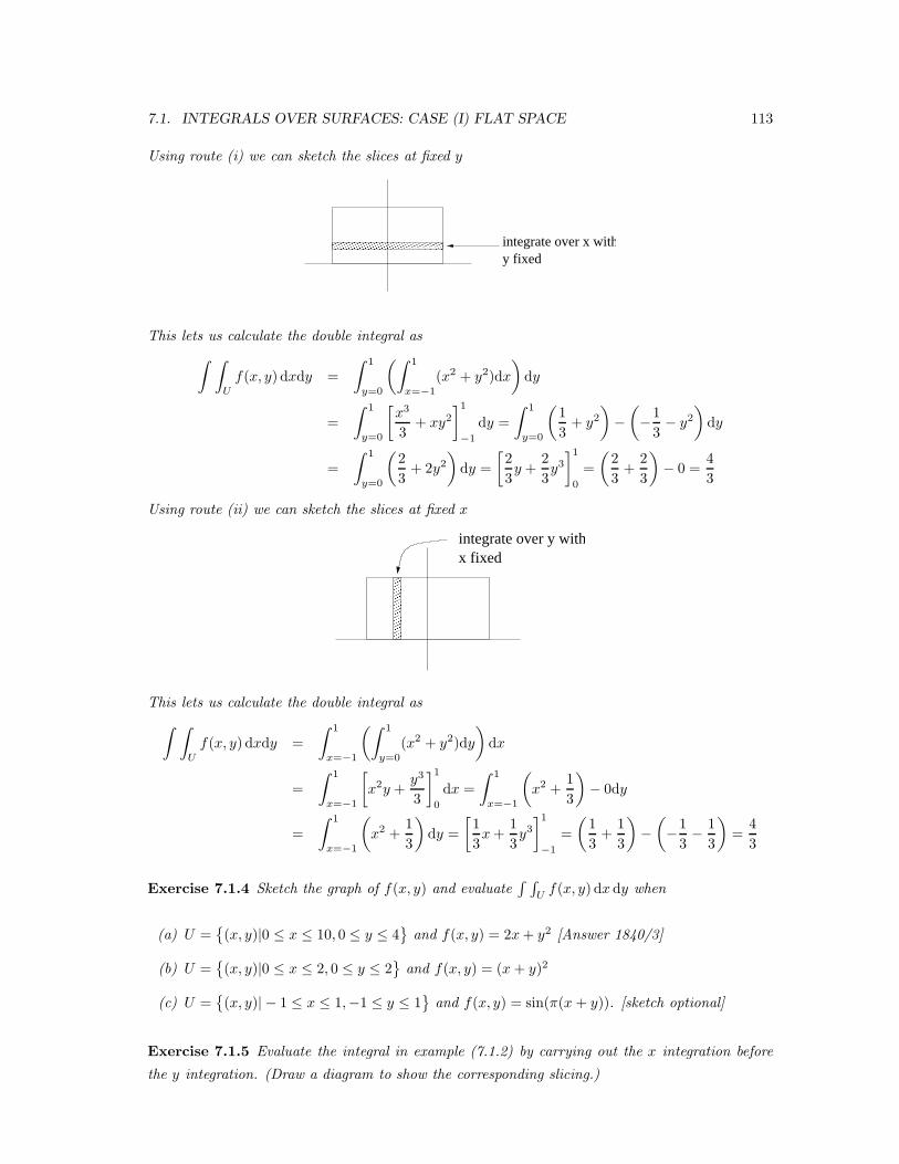
7.1. INTEGRALS OVER SURFACES: CASE (I) FLAT SPACE 113
Using route (i) we can sketch the slices at fixed y
y fixedintegrate over x with
This lets us calculate the double integral as
∫ ∫
U
f(x, y) dxdy =
∫ 1
y=0
(∫ 1
x=−1
(x2 + y2)dx
)
dy
=
∫ 1
y=0
[x3
3+ xy2
]1
−1
dy =
∫ 1
y=0
(1
3+ y2
)
−(
−1
3− y2
)
dy
=
∫ 1
y=0
(2
3+ 2y2
)
dy =
[2
3y +
2
3y3]1
0
=
(2
3+
2
3
)
− 0 =4
3
Using route (ii) we can sketch the slices at fixed x
x fixedintegrate over y with
This lets us calculate the double integral as
∫ ∫
U
f(x, y) dxdy =
∫ 1
x=−1
(∫ 1
y=0
(x2 + y2)dy
)
dx
=
∫ 1
x=−1
[
x2y +y3
3
]1
0
dx =
∫ 1
x=−1
(
x2 +1
3
)
− 0dy
=
∫ 1
x=−1
(
x2 +1
3
)
dy =
[1
3x+
1
3y3]1
−1
=
(1
3+
1
3
)
−(
−1
3− 1
3
)
=4
3
Exercise 7.1.4 Sketch the graph of f(x, y) and evaluate∫ ∫
Uf(x, y) dx dy when
(a) U =(x, y)|0 ≤ x ≤ 10, 0 ≤ y ≤ 4
and f(x, y) = 2x+ y2 [Answer 1840/3]
(b) U =(x, y)|0 ≤ x ≤ 2, 0 ≤ y ≤ 2
and f(x, y) = (x + y)2
(c) U =(x, y)| − 1 ≤ x ≤ 1,−1 ≤ y ≤ 1
and f(x, y) = sin(π(x + y)). [sketch optional]
Exercise 7.1.5 Evaluate the integral in example (7.1.2) by carrying out the x integration before
the y integration. (Draw a diagram to show the corresponding slicing.)
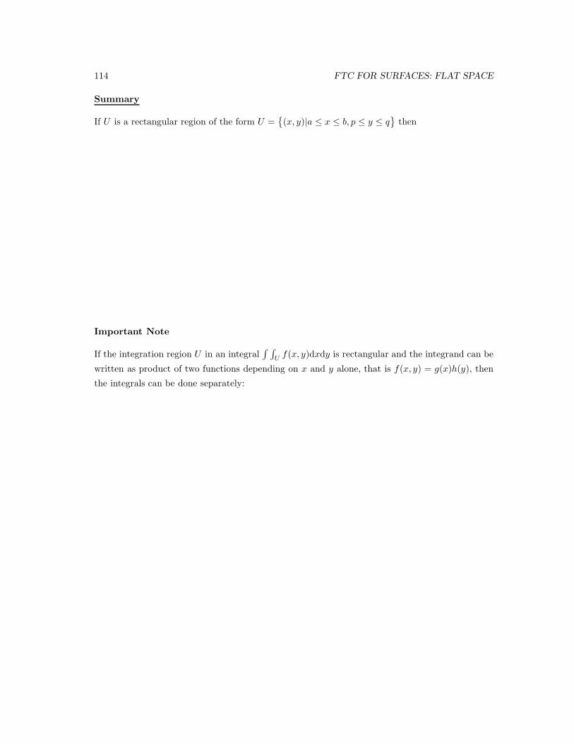
114 FTC FOR SURFACES: FLAT SPACE
Summary
If U is a rectangular region of the form U =(x, y)|a ≤ x ≤ b, p ≤ y ≤ q
then
Important Note
If the integration region U in an integral∫ ∫
Uf(x, y)dxdy is rectangular and the integrand can be
written as product of two functions depending on x and y alone, that is f(x, y) = g(x)h(y), then
the integrals can be done separately:
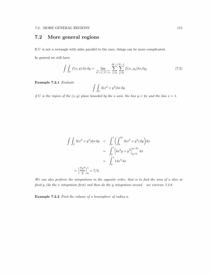
7.2. MORE GENERAL REGIONS 115
7.2 More general regions
If U is not a rectangle with sides parallel to the axes, things can be more complicated.
In general we still have
∫ ∫
U
f(x, y) dxdy = limδx→0,δy→0
M→∞,N→∞
M−1∑
i=0
N−1∑
j=0
f(xi, yj)δxiδyj (7.2)
Example 7.2.1 Evaluate ∫ ∫
U
3(x2 + y2)dxdy
if U is the region of the (x, y) plane bounded by the x-axis, the line y = 2x and the line x = 1.
∫ ∫
U
3(x2 + y2)dx dy =
∫ 1
0
(∫ 2x
0
3(x2 + y2) dy
)
dx
=
∫ 1
0
[
3x2y + y3]y=2x
y=0dx
=
∫ 1
0
14x3 dx
=[7x4
2
]1
0= 7/2.
We can also perform the integrations in the opposite order, that is to find the area of a slice at
fixed y (do the x integration first) and then do the y integration second – see exercise 7.2.6
Example 7.2.2 Find the volume of a hemisphere of radius a.
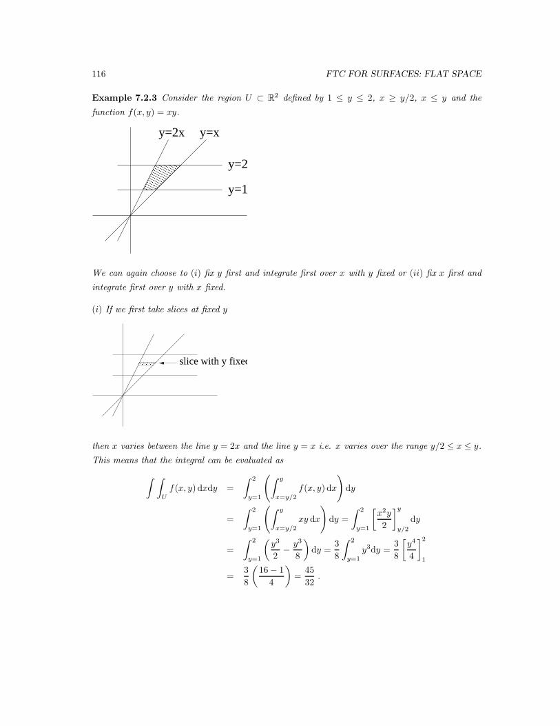
116 FTC FOR SURFACES: FLAT SPACE
Example 7.2.3 Consider the region U ⊂ R2 defined by 1 ≤ y ≤ 2, x ≥ y/2, x ≤ y and the
function f(x, y) = xy.
y=1
y=2x y=x
y=2
We can again choose to (i) fix y first and integrate first over x with y fixed or (ii) fix x first and
integrate first over y with x fixed.
(i) If we first take slices at fixed y
slice with y fixed
then x varies between the line y = 2x and the line y = x i.e. x varies over the range y/2 ≤ x ≤ y.
This means that the integral can be evaluated as
∫ ∫
U
f(x, y) dxdy =
∫ 2
y=1
(∫ y
x=y/2
f(x, y) dx
)
dy
=
∫ 2
y=1
(∫ y
x=y/2
xy dx
)
dy =
∫ 2
y=1
[x2y
2
]y
y/2
dy
=
∫ 2
y=1
(y3
2− y3
8
)
dy =3
8
∫ 2
y=1
y3dy =3
8
[y4
4
]2
1
=3
8
(16− 1
4
)
=45
32.
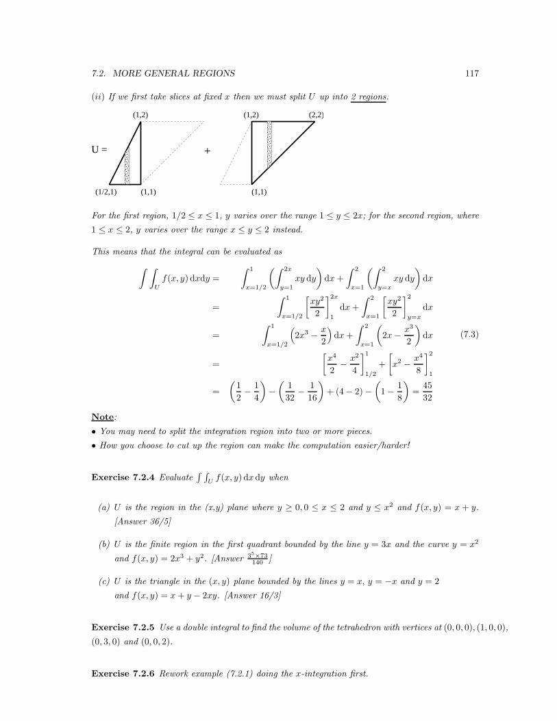
7.2. MORE GENERAL REGIONS 117
(ii) If we first take slices at fixed x then we must split U up into 2 regions.
+
U =
(1/2,1) (1,1) (1,1)
(1,2)(1,2) (2,2)
For the first region, 1/2 ≤ x ≤ 1, y varies over the range 1 ≤ y ≤ 2x; for the second region, where
1 ≤ x ≤ 2, y varies over the range x ≤ y ≤ 2 instead.
This means that the integral can be evaluated as
∫ ∫
U
f(x, y) dxdy =
∫ 1
x=1/2
(∫ 2x
y=1
xy dy
)
dx+
∫ 2
x=1
(∫ 2
y=x
xy dy
)
dx
=
∫ 1
x=1/2
[xy2
2
]2x
1
dx+
∫ 2
x=1
[xy2
2
]2
y=x
dx
=
∫ 1
x=1/2
(
2x3 − x
2
)
dx+
∫ 2
x=1
(
2x− x3
2
)
dx
=
[x4
2− x2
4
]1
1/2
+
[
x2 − x4
8
]2
1
=
(1
2− 1
4
)
−(
1
32− 1
16
)
+ (4− 2)−(
1− 1
8
)
=45
32
(7.3)
Note:
• You may need to split the integration region into two or more pieces.
• How you choose to cut up the region can make the computation easier/harder!
Exercise 7.2.4 Evaluate∫ ∫
Uf(x, y) dxdy when
(a) U is the region in the (x,y) plane where y ≥ 0, 0 ≤ x ≤ 2 and y ≤ x2 and f(x, y) = x + y.
[Answer 36/5]
(b) U is the finite region in the first quadrant bounded by the line y = 3x and the curve y = x2
and f(x, y) = 2x3 + y2. [Answer 35×73140 ]
(c) U is the triangle in the (x, y) plane bounded by the lines y = x, y = −x and y = 2
and f(x, y) = x+ y − 2xy. [Answer 16/3]
Exercise 7.2.5 Use a double integral to find the volume of the tetrahedron with vertices at (0, 0, 0), (1, 0, 0),
(0, 3, 0) and (0, 0, 2).
Exercise 7.2.6 Rework example (7.2.1) doing the x-integration first.
118 FTC FOR SURFACES: FLAT SPACE
7.2.1 Areas of regions from double integrals
Double integrals may also be used to calculate areas of regions in the (x, y) plane. The key formula
is:
Area of U =
∫ ∫
U
1 dxdy (7.4)
Example 7.2.7 Use double integration to calculate the area of U where U is the region bounded
by the axes and the line y + 2x = 6
Exercise 7.2.8 Use double integration to calculate the area of U where U is the disc x2 + y2 ≤ 9
Example 7.2.9 Find the area of the ellipse x2/a2 + y2/b2 = 1 in R2.
7.3 Changing variables
As is often the case, a difficult problem may be made simpler if the coordinates are well chosen.
This is equally so for double integrals, the choice of coordinate system may have a radical effect
on how difficult or easy the integrals is to evaluate. For example, the double integral we have just
looked at to compute the area of a disc is much simpler in polar coordinates. One of the skills to
develop is how to choose a ‘good’ coordinate system – this will depend on the function you are
integrating and the shape of the region over which you are integrating.
We begin with a reminder about the change of variable rule for single integrals. Suppose that
u = u(x) and that as x increases from a to b then u(x) increases from p to q. Then
∫ b
a
f(x)dx =
∫ q
p
f(x(u))dx
dudu. (7.5)
When proving this result the key point is that δx ≈ dx
duδu so that We are going to derive the
7.3. CHANGING VARIABLES 119
analogous rule for double integrals. To illustrate the ideas involved we will consider the following
problem:
Example 7.3.1 Evaluate∫ ∫
U (x+ y)2 dxdy where U is the region bounded by the lines x+ y = 0,
x+ y = 2, 2y − x = 0 and 2y − x = −4.
It would be possible (but unnecessarily laborious) to evaluate this integral by direct means. Change
of variable makes it much simpler.
120 FTC FOR SURFACES: FLAT SPACE
The method for changing variables in a double integral is summarised in the following theorem:
Theorem 7.3.2 Suppose that the pair of functions u = u(x, y) and v = v(x, y) are invertible so
that x = x(u, v) and y = y(u, v). Also suppose that the region U in the (x, y)-plane corresponds to
the region U ′ in the (u, v)-plane. Then∫ ∫
U
f(x, y) dxdy =
∫ ∫
U ′
f(x(u, v), y(u, v))∣∣∣∂(x, y)
∂(u, v)
∣∣∣ dudv (7.6)
where∂(x, y)
∂(u, v)= det
(∂ x∂ u
∂ y∂ u
∂ x∂ v
∂ y∂ v
)
. (7.7)
Note that in the integrand it is the modulus of the Jacobian ∂(x,y)∂(u,v) .
The next example uses this theorem.
Example 7.3.3 Evaluate∫ ∫
Uxy dxdy where U is the region in the first quadrant bounded by
x2 + y2 = 9, x2 + y2 = 25, x2 − y2 = 1, x2 − y2 = 9.
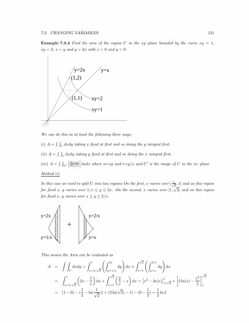
7.3. CHANGING VARIABLES 121
Example 7.3.4 Find the area of the region U in the xy–plane bounded by the curve xy = 1,
xy = 2, x = y and y = 2x with x > 0 and y > 0.
(1,2)
xy=2
xy=1
y=2x y=x
(1,1)
We can do this in at least the following three ways:
(i) A =∫ ∫
U dxdy taking x fixed at first and so doing the y integral first.
(ii) A =∫ ∫
Udxdy taking y fixed at first and so doing the x integral first.
(iii) A =∫ ∫
U ′
∣∣∣∂(x,y)∂(u,v)
∣∣∣ dudv where u=xy and v=y/x and U ′ is the image of U in the uv–plane
Method (i)
In this case we need to split U into two regions On the first, x varies over [ 1√2, 1] and on this region
for fixed x, y varies over 1/x ≤ y ≤ 2x. On the second, x varies over [1,√2] and on this region
for fixed x, y varies over x ≤ y ≤ 2/x.
y=2/x
y=x
+
y=1/x
y=2x
This means the Area can be evaluated as
A =
∫ ∫
U
dxdy =
∫ 1
x=1/√2
(∫ 2x
y=1/x
dy
)
dx+
∫√2
x=1
(∫ 2/x
y=x
dy
)
dx
=
∫ 1
x=1/√2
(
2x− 1
x
)
dx+
∫√2
x=1
(2
x− x
)
dx =[x2 − ln(x)
]1
1/√2+
[
2 ln(x)− x2
2
]√2
1
= (1− 0)− (1
2− ln(
1√2)) + (2 ln(
√2)− 1)− (0− 1
2) =
1
2ln 2
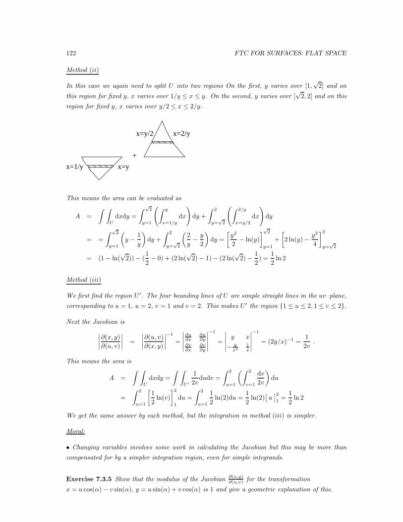
122 FTC FOR SURFACES: FLAT SPACE
Method (ii)
In this case we again need to split U into two regions On the first, y varies over [1,√2] and on
this region for fixed y, x varies over 1/y ≤ x ≤ y. On the second, y varies over [√2, 2] and on this
region for fixed y, x varies over y/2 ≤ x ≤ 2/y.
+
x=y/2 x=2/y
x=1/y x=y
This means the area can be evaluated as
A =
∫ ∫
U
dxdy =
∫√2
y=1
(∫ y
x=1/y
dx
)
dy +
∫ 2
y=√2
(∫ 2/y
x=y/2
dx
)
dy
= =
∫√2
y=1
(
y − 1
y
)
dy +
∫ 2
y=√2
(2
y− y
2
)
dy =
[y2
2− ln(y)
]√2
y=1
+
[
2 ln(y)− y2
4
]2
y=√2
= (1 − ln(√2))− (
1
2− 0) + (2 ln(
√2)− 1)− (2 ln(
√2)− 1
2) =
1
2ln 2
Method (iii)
We first find the region U ′. The four bounding lines of U are simple straight lines in the uv–plane,
corresponding to u = 1, u = 2, v = 1 and v = 2. This makes U ′ the region 1 ≤ u ≤ 2, 1 ≤ v ≤ 2.
Next the Jacobian is
∣∣∣∣
∂(x, y)
∂(u, v)
∣∣∣∣
=
∣∣∣∣
∂(u, v)
∂(x, y)
∣∣∣∣
−1
=
∣∣∣∣∣
∂u∂x
∂u∂y
∂v∂x
∂v∂y
∣∣∣∣∣
−1
=
∣∣∣∣∣
y x
− yx2
1x
∣∣∣∣∣
−1
= (2y/x)−1 =1
2v.
This means the area is
A =
∫ ∫
U
dxdy =
∫ ∫
U ′
1
2vdudv =
∫ 2
u=1
(∫ 2
v=1
dv
2v
)
du
=
∫ 2
u=1
[1
2ln(v)
]2
1
du =
∫ 2
u=1
1
2ln(2)du =
1
2ln(2)
[u]2
1=
1
2ln 2
We get the same answer by each method, but the integration in method (iii) is simpler.
Moral:
• Changing variables involves some work in calculating the Jacobian but this may be more than
compensated for by a simpler integration region, even for simple integrands.
Exercise 7.3.5 Show that the modulus of the Jacobian ∂(x,y)∂(u,v) for the transformation
x = u cos(α)− v sin(α), y = u sin(α) + v cos(α) is 1 and give a geometric explanation of this.
7.4. POLAR COORDINATES 123
Exercise 7.3.6 By using an appropriate change of variables, evaluate∫ ∫
U sin(x + 2y) cos(x −y) dxdy where U is the region bounded by x+ 2y = 0, x+ 2y = π, x− y = 0 and x− y = π
2 .
7.4 Polar coordinates
One of the most frequent change of variables used is from Cartesian to polar coordinates, possibly
slightly adapted to a specific situation. In two dimensions polar coordinates are useful if the region
has some circular properties, such as a disc, or the integrand has a simple expression in terms of
r2 = x2 + y2 and θ.
To use polar coordinates for integration, we need to compute the Jacobian:
We can now use them to calculate, for example, the area of a disk of radius R, centered at the
origin:
124 FTC FOR SURFACES: FLAT SPACE
Sometimes one has to move the origin as well.
Example 7.4.1 Evaluate∫ ∫
U xy dxdy where U is the region where x2 + 2x+ y2 − 6y ≤ 6.
With double integration some integrals lend themselves to the use of polar coordinates, or to
slightly modified versions for elliptical regions.
Example 7.4.2 Evaluate using a double integral the area of the region U enclosed by the ellipse
x2
α2+y2
β2= 1 ,
where α > 0, β > 0 are positive constants.
Notice that in this example if we set α = β = 1 then we get back to first computation we did of
the area of a disc and the case of standard polar coordinates.
7.4. POLAR COORDINATES 125
Example 7.4.3 Evaluate∫ +∞−∞ e−x2
dx.
(The solution to this example is a key result which you will find coming up in other contexts. It
cannot be evaluated analytically as an integral of 1-variable, but can nevertheless be computed
through an elegant artifice using polar coordinates and double integrals. It can also be evaluated
by ‘contour integration’.)
126 FTC FOR SURFACES: FLAT SPACE
Example 7.4.4 Evaluate ∫ ∫
U
x√
x2 + y2dx dy
where U is the region bounded by x = 0, y = 2 and y = x.
Exercise 7.4.5 Sketch the graph of r = 2 + cos θ + sin θ and calculate the area it encloses.
Exercise 7.4.6 Suppose U is the region in the (x, y)-plane where x ≥ 0, y ≥ 0 and x2 + y2 ≤ 5.
Sketch U and use polar coordinates to evaluate∫ ∫
U
√
x2 + y2 dxdy. [Answer 5√5π6 ]
Exercise 7.4.7 Use polar coordinates to evaluate the integral in example 7.2.1.
[Hint: to do the θ integration make the substitution u = tan θ.]
Exercise 7.4.8 Sketch the cardioid r = 1 + cosθ, 0 ≤ θ ≤ 2π and calculate its area.
Exercise 7.4.9 Find the area of one petal of the curve r = sin 3θ. [Answer π/12]
7.5. FTC II: GREEN’S THEOREM 127
7.5 FTC II: Green’s theorem
We have seen that when the integrand is the gradient of a function, a line integral around a closed
curve in R3 is zero, see Corollary 6.4.3. In general of course the integrand will not be a gradient.
Green’s theorem relates the integral around a closed curve C which lies in a flat plane R2 to a
double integral over the 2-dimensional region Ω bounded by C. It is a nice theorem, of great use;
its discoverer, Green, was a miller from Nottingham who also discovered ‘Green’s functions’ which
are of great use in solving partial differential equations, quantum field theory etc etc.
Theorem 7.5.1 (FTC II) Let C be a simple closed curve in R2 and Ω be the interior of C. Also
let v : R2 −→ R2 be a vector field on R2, given in components by v(x, y) = P (x, y)i + Q(x, y)j.
Then, if C is parametrised in an anti-clockwise direction,
∫ ∫
Ω
(∂ Q
∂ x− ∂ P
∂ y
)
dxdy =
∮
C
P dx+Q dy =
∮
v · dr (7.8)
Proof:
128 FTC FOR SURFACES: FLAT SPACE
Example 7.5.2 Verify Green’s theorem when C is the circle r(t) = cos ti+ sin tj, 0 ≤ t ≤ 2π and
v(x, y) = yi+ 2xj.
Two of the uses of Green’s theorem are to simplify integrals and to establish relationships between
(for example, physical) quantities.
Example 7.5.3 Evaluate∮
C(xi − yj) · dr where C is the circle (x− 3)2 + (y − 7)2 = 49.
Here is a cautionary example
Exercise 7.5.4 Show that Green’s theorem is apparently violated when C is the circle x2 + y2 = 1
and v is the vector field
v(x, y) =−y
x2 + y2i+
x
x2 + y2j.
Explain why in fact there is no contradiction.
7.5. FTC II: GREEN’S THEOREM 129
Green’s Theorem can be given the following ‘invariant’ form (meaning we do not have to mention
the components P,Q).
Corollary 7.5.5 (FTC II) With the assumptions of Theorem 7.5.1, the equality (7.8) can be
restated as ∫ ∫
Ω
(∇× v) · k dxdy =
∮
C
v · dr . (7.9)
In particular, this provides a second proof of Corollary 6.4.3 for the case where C is a simple closed
curve in R2. That is, for any scalar function f : R2 → R1
∮
C
∇f · dr = 0
Conversely, if there is a simple closed curve C such that∮
C
v · dr 6= 0 , (7.10)
then v is not a gradient vector field – that is, in this case, v 6= ∇f for any scalar function
f : R2 −→ R1.
130 FTC FOR SURFACES: FLAT SPACE
. Proof:
Example 7.5.6 Use both Green’s Theorem and also a direct method to show that the vector field
v(v, y) = −yi+ xj on R2 is not a gradient vector field.
A beautiful theorem about integration on surfaces tells that in fact the formula (7.9) generalises
to curved 2-dimensional spaces, such as a hemisphere. That theorem is Stokes’ Theorem, and to
formulate it we need to generalise our ideas about integration from flat 2-dimensional regions to
curved 2-dimensional spaces. This is what we do next.
131
Chapter 8
FTC for Surfaces: Curved Space
8.1 Integrals over Surfaces: Case (II) curved space
The aim of this section is to show what a double integral over a curved surface S embedded in R3
such as ∫ ∫
S
g dσ (8.1)
means, how it may be evaluated and what use it might be.
The definition of (8.1) generalises the ideas of Section 7.1 in the same way that in Chapter 6 the
definition of an integral over any curve sitting in R3 generalised ideas about integration over the
flat curve [a, b].
The basic idea is that (8.1) can be thought of as the volume of the 3-dimensional strip between S
and the graph of g restricted to S:
132 FTC FOR SURFACES: CURVED SPACE
The formal definition is then
Definition 8.1.1 Let S be a surface in R3 of finite extent and g : R3 −→ R1 a scalar function.
Then∫ ∫
S
g dσ = limN,M−→∞
N−1∑
i=0
M=1∑
j=0
g(ri,j) δσi,j . (8.2)
When it comes to actually evaluating such an integral, a different method is used.
8.2 Parameterisations of Surfaces: Coordinates
What you need in order to evaluate a surface integral
To evaluate an integral over a path we had to choose a parametrisation for the path. Likewise with
surfaces, to compute the abstract quantity (8.2) we have to choose a parametrisation — in other
words, we choose “coordinates” for S. For example, lines of latitude and longitude can be used to
specify a position on the surface of the Earth, these are just spherical polar coordinates (ρ, θ, φ)
with ρ constant, equal to ‘the’ radius of the Earth.
This is the subject of this section.
Defining coordinates on a surface is very important: this enables us to actually carry out com-
putations, such as double-integrals to compute surface area. An example of coordinates for a
2-dimensional space are the lines of latitude and longitude used to specify a position on the sur-
face of the Earth. (This is a particular coordinate system for the 2-sphere called ‘spherical polar
coordinates with constant radius’ — more on that shortly).
If you look back at section 2.1.2 where we defined a coordinate on a (1-dimensional) curve, you
will see that that meant giving a bijective (1-1 and onto) function from a subset R1 to the curve.
8.2. PARAMETERISATIONS OF SURFACES: COORDINATES 133
Similarly, to parametrise a surface (which is a 2-dimensional object) we need such a map from a
subset of R2:
Definition 8.2.1 A parametrisation of a surface S ⊂ R3 means a differentiable map from a region
U ⊂ R2 to S
r : U ⊂ R2 −→ S ⊂ R
3 , (u, v) 7−→ r(u, v) ,
which is onto and one-to-one except possible on a ‘line of points’.
The simplest case of a surface is a plane, even the xy-plane which we can think of as R2. When
we refer to R2 we already have the basic Cartesian, or ‘rectangular’, coordinates.
But these are not always a good choice of coordinate to perform computations – such as 2-
dimensional integrals (these will be defined in a later Chapter)– or for writing down equations,
such as the equations of a surface.
One well-known system of coordinates in R2 are polar coordinates, or ‘circular’ coordinates.
134 FTC FOR SURFACES: CURVED SPACE
Example 8.2.2 Polar coordinates
However, there are an infinite variety of different coordinate systems in R2 (a coordinate system
for R2 is a way of assigning uniquely two numbers (a, b) to each point of R2).
Example 8.2.3 Sketch the coordinate system u = x+ y, v = 2y − x.
8.2. PARAMETERISATIONS OF SURFACES: COORDINATES 135
Example 8.2.4
Sketch the alternative coordinate system (r, θ) for plane R2, where r ≥ 0, 0 ≤ θ ≤ 2π ,
x = 2r cos θ + 1, y = 3r sin θ − 2
Example 8.2.5 It is not hard to find parameterisations of any plane in R3
136 FTC FOR SURFACES: CURVED SPACE
Now think about curved surfaces: the surface S defined by x2 + y2 + z2 = 1 can be parameterised
by
r : [0, π]× [0, 2π] −→ S ⊂ R3 (θ, φ) 7−→ r(θ, φ) ,
using two parameters θ and φ
r(θ, φ) = sin θ cosφi + sin θ sinφj+ cos θk . (8.3)
This is easily modified to parameterise a sphere of radius ρ > 0 with centre at (x0, y0, z0).
Notice there is a line of points where r is not bijective.
8.2. PARAMETERISATIONS OF SURFACES: COORDINATES 137
8.2.1 Parametrising graph-surfaces
An important way in which surfaces enter into our studies here are as graphs of scalar valued
functions f : R2 −→ R1. That is, such a surface S is the subset of R3
Graph(f) = (x, y, z)|z = f(x, y)
In this case, one method for parametrising the surface is to use x and y as parameters and
r(x, y) = xi + yj+ f(x, y)k. (8.4)
Example 8.2.6 Show that the portion of the sphere of radius 3, centre the origin which lies in the
region z ≥ 0 may be parametrised as
r(x, y) = xi+ yj+√
9− x2 − y2k, x2 + y2 ≤ 9. (8.5)
(Note that usually the values of the parameters have to be restricted to some subset Ω of R2. In
this example Ω is the disc x2 + y2 ≤ 9.)
138 FTC FOR SURFACES: CURVED SPACE
Example 8.2.7 Show that the portion of the sphere of radius 3, centre the origin which lies in the
region z ≥ 0 may be parametrised as
r(x, y) = xi+ yj+√
9− x2 − y2k, x2 + y2 ≤ 9. (8.6)
Exercises
Exercise 8.2.8 Show that the plane x+ 2y − 3z = 5 may be parametrised by
x = 6t− 10s+ 5, y = 5s, z = 2t.
Find a different parametrisation of this plane.
Exercise 8.2.9 Describe the surface parametrised by
x = cos t, y = sin t, z = s, 0 ≤ s ≤ 1, 0 ≤ t ≤ 2π.
8.3. THE FUNDAMENTAL VECTOR PRODUCT OF A SURFACE 139
8.3 The fundamental vector product of a surface
Once we have a parametrisation of S we can calculate the ‘fundamental vector product’ N(u, v) ∈R3 at each point p = r(u, v) ∈ S. This vector product defines a vector field which is normal to the
surface S at each point and where ‖N(u, v)‖ is the area of an infinitesimal parallelogram in the
tangent space TpS to S at p.
140 FTC FOR SURFACES: CURVED SPACE
Definition 8.3.1 Let
r(u, v) = x(u, v)i + y(u, v)j+ z(u, v)k
be a parametrised surface, and
r′u(u, v) =∂ x
∂ u(u, v)i+
∂ y
∂ u(u, v)j+
∂ z
∂ u(u, v)k
and
r′v(u, v) =∂ x
∂ v(u, v)i+
∂ y
∂ v(u, v)j+
∂ z
∂ v(u, v)k
be partial derivatives of r with respect to u and v respectively. Then the vector
N(u, v) = r′u(u, v)× r′v(u, v)
is known as the ‘fundamental vector product’ of the surface at the point r(u, v).
Theorem 8.3.2 The fundamental vector product N(u, v) is perpendicular to the surface at r(u, v).
8.3. THE FUNDAMENTAL VECTOR PRODUCT OF A SURFACE 141
Corollary 8.3.3 If the surface S is described by the equation z = f(x, y), then it can be parametrised
as
r(x, y) = xi+ yj+ f(x, y)k (8.7)
as we have seen before. In this case
N(x, y) = −∂ f∂ x
i− ∂ f
∂ yj+ k. (8.8)
142 FTC FOR SURFACES: CURVED SPACE
Example 8.3.4 Find the fundamental vector product of the plane
r(u, v) = (u + v)i+ (3u− 2v)j+ (v − u)k.
Example 8.3.5 Compute the fundamental vector product to the sphere of radius 2 centred at the
origin .
8.4. EVALUATING SURFACE INTEGRALS AND SURFACE AREA 143
8.4 Evaluating Surface Integrals and Surface area
With a parametrisation of the surface S at hand, we obtain the following formula for a surface
integral:
Proposition 8.4.1 For a scalar function g : R3 −→ R1 and a surface parametrised by u and v,∫ ∫
S
g dσ =
∫ ∫
Ω
g(r(u, v)) ‖N(u, v)‖ dudv.
Corollary 8.4.2 If S is parametrised as the graph of a function f : U ⊂ R2 −→ R1, we then have
∫ ∫
S
f dσ =
∫ ∫
Ω
f(x, y)
√
1 +
(∂f
∂x
)2
+
(∂f
∂y
)2
dx dy .
144 FTC FOR SURFACES: CURVED SPACE
One of the uses of a surface integral is to calculate the area of a surface.
Theorem 8.4.3 Suppose that S = r(u, v), (u, v) ∈ Ω is a parametrised surface. Then
Area of S =
∫ ∫
Ω
|N(u, v)| du dv. (8.9)
Corollary 8.4.4 If the surface S is described by the equation z = f(x, y), (x, y) ∈ Ω, then
Area of S =
∫ ∫
Ω
√(
(∂ f
∂ x(x, y))2 + (
∂ f
∂ y(x, y))2 + 1
)
dx dy. (8.10)
Notation: the infinitesimal area |N(u, v)| du dv is often written dσ. It is the analogue for surfaces
of the infinitesimal arc length ds = |r′(t)| dt for a curve.
8.4. EVALUATING SURFACE INTEGRALS AND SURFACE AREA 145
Example 8.4.5 Find the area of the part of the surface z2 = x2 + y2 enclosed between the planes
z = 0 and z = 4.
Exercise 8.4.6 Use the preceding theorem to show that the area of a sphere of radius 3 is 36π.
Exercise 8.4.7 Prove this corollary, using equation (8.8).
Exercise 8.4.8 Find the area of the portion of the plane x+y+z = 4 that lies within the cylinder
x2 + y2 = 4.
Exercise 8.4.9 Find the area of the portion of the sphere z =√
1− x2 − y2 which lies between
the planes z = 0 and z = 1.
146 FTC FOR SURFACES: CURVED SPACE
8.5 Surface Integrals of Vector Fields
Just as we extended in Chapter 6 the definition of integrals of functions over paths to integrals of
vector fields over paths, we can also easily extend our definition here to integrals of vector fields
over surfaces.
Definition 8.5.1 Let S be a surface in R3 of finite extent and let v : R3 −→ R3 be a vector field
on R3. Also suppose that at each point of S n is a unit vector normal to S. Then the integral of
v over S — or, the flux of v across S in the direction of n — is defined by
∫ ∫
S
v · n dσ = limN,M−→∞
N∑
i=0
M∑
j=0
v(ui, vi) · n(ui, vi)δσi,j . (8.11)
Thus the flux is the integral over the surface of the component of the vector field normal to the
surface at each point. (You may have come across the idea of the flux of a field in electromagnetism.)
This kind of surface integral appears in the two further integral theorems (Stokes’ theorem and
the divergence theorem) which form the final part of this course.
8.5. SURFACE INTEGRALS OF VECTOR FIELDS 147
When actually calculating a flux we use a parametrisation of the surface S. We then obtain the
following formula for the vector ndσ:
Proposition 8.5.2 For a surface parametrised by u and v,
ndσ := N(u, v)dudv.
Hence ∫ ∫
S
v · ndσ =
∫ ∫
Ω
v ·N(u, v)dudv.
Example 8.5.3 Evaluate the flux of v(x, y, z) = xi+ yj out of the surface S which is the sphere
x2 + y2 + z2 = 1.
First parametrise the surface. (This is simpler in this case than solving for z.)
Next find N(u, v).
148 FTC FOR SURFACES: CURVED SPACE
Finally evaluate the flux
In order to calculate the flux of a vector field over a surface given by an equation z = f(x, y), the
following proposition is useful:
Proposition 8.5.4 If v is a vector field on R3 and S is the surface determined by the equation
z = f(x, y), (x, y) ∈ Ω,
then the flux of v = v1i+ v2j+ v3k across S in the direction of the upwards normal is
∫ ∫
S
v.n dσ =
∫ ∫
Ω
(
−v1∂ f
∂ x− v2
∂ f
∂ y+ v3
)
dxdy. (8.12)
8.5. SURFACE INTEGRALS OF VECTOR FIELDS 149
Example 8.5.5 Calculate the flux of v = xi+ yj+ zk out of the surface S where S is the portion
of the elliptic paraboloid z = 9− (x2 + y2) for which z ≥ 0.
Exercise 8.5.6 Calculate the flux of v = yi+ xj upwards across the hemisphere
z =√
1− x2 − y2 z ≥ 0.
SOME NOTATIONAL VARIATIONS: In some texts you will find
dA used to denote dx dy, the infinitesimal area element in the (x, y)-plane
dv used to denote dx dy dz, the infinitesimal volume element in (x, y, z)-space and
dS to denote ndσ.
150 FTC FOR SURFACES: CURVED SPACE
8.6 Stokes’ theorem
Stokes’ theorem is an integral theorem which is a generalisation of Green’s theorem.
Theorem 8.6.1 Suppose that S is a curved region in R3 bounded by the closed curve C. Then∫ ∫
S
(∇× v) · n dσ =
∮
C
v · dr (8.13)
where C is taken anti-clockwise about n.
Notice, then, the Theorem says that for any vector field v on R3 we can compute∮
Cv · dr by
evaluating∫ ∫
S(∇× v) · n dσ for any such surface S ! Proof:
8.6. STOKES’ THEOREM 151
Example 8.6.2 Verify Stokes’ theorem if S is the portion of the elliptic paraboloid z = 9−(x2+y2)
for which z ≥ 0 and v is the vector field yi− xj.
Example 8.6.3 Calculate ∫ ∫
S
(∇× v) · n dσ
(a) directly and (b) using Stokes’ theorem when
S is the upper half of the unit sphere centre the origin and v = z2i+ 2xj+ y3k.
Example 8.6.4 Calculate ∫ ∫
S
(∇× v) · n dσ
(a) directly and (b) using Stokes’ theorem when
S is the region of the surface z = (z2 + y2 − 1)2 contained inside the cylinder x2 + y2 = 1 and
v = (z + 1)(−yi+ xj).
152 FTC FOR SURFACES: CURVED SPACE
We can conclude with the following interesting properties — compare these with those at the end
of the previous Chapter.
Corollary 8.6.5 Suppose that the surface S is closed; that is, it is contained in a finite region of
space and has no boundary (such as a sphere). Then
∫ ∫
S
(∇× v) · n dσ = 0 . (8.14)
Conversely, if F is a vector field and there exists a closed surface S such that∫ ∫
S
F · n dσ 6= 0 , (8.15)
then F is not the curl of any vector field in R3, i.e. F 6= ∇× u any vector field u.
8.6. STOKES’ THEOREM 153
The next one is similar but more demanding:
Corollary 8.6.6 Suppose that the surface S has two closed boundary curves C1 and C2 (for ex-
ample, when S is a cylinder with two circles as boundary). Then
∫ ∫
S
(∇× v) · n dσ =
∮
C1
v · dr−∮
C2
v · dr (8.16)
where C1 is taken anti-clockwise about n and C2 is taken clockwise about n.
On the other hand, we can evaluate∮
C1
v · dr −∮
C2
v · dr by computing∫ ∫
S(∇ × v) · n dσ over
any such surface S.
154 FTC FOR SURFACES: CURVED SPACE
To finish off, here’s a past Final Exam question:
Let P be the surface in R3 which is the graph of the function f(x, y) = 1 − x2 − y2 and let S be
the portion of P for which z ≥ 0. Let C be the curve which is the intersection of P with the plane
z = 0.
(a) Sketch S and C on one diagram.
(b) Show that S has areaπ
6(5√5− 1) .
(c) Let v : R3 −→ R3 be the vector field
v = (x − y3) i+ (x3 + y) j+ z3xy k .
(i) Calculate ∇× v.
(ii) Let D denote the region in the (x, y)-plane for which x2 + y2 ≤ 1. Use Stokes’ Theorem
to show that ∫ ∫
S
∇× v · n dσ =
∫ ∫
D
∇× v · k dxdy ,
where n is the outward unit normal vector field to the surface S and dσ is the area
element of S.
(iii) Show that∫ ∫
S
∇× v · n dσ =3π
2.
(iv) Hence, or otherwise, prove that there does not exist any function f : R3 −→ R1 for
which ∇f = v.
8.7. MISCELLANEOUS EXERCISES 155
8.7 Miscellaneous Exercises
Exercise 8.7.1 From Final Exam 2003
Suppose that in the positive quadrant x > 0, y > 0 of R2 ,
u(x, y) =y2
xand v(x, y) = xy .
(i) Calculate the Jacobian∣∣∣∣
∂(x, y)
∂(u, v)
∣∣∣∣.
(ii) Hence evaluate the integral
∫ ∫
U
y2
xlog
(y2
x
)
dxdy ,
where U is the region of R2 bounded by the curves y2 = x, y2 = 2x, xy = 1 and xy = 2.
Exercise 8.7.2 From Final Exam 2003:
Let C be the circle x2 + y2 = 4. Using Green’s Theorem, or otherwise, show that∮
C
(sinx− y3)dx+ (cos y + x3)dy = 24π ,
where the integration is carried out in the anticlockwise direction.
Exercise 8.7.3 Compute the surface integral
∫∫
S
v.n dσ, where n is the upward unit normal to
the surface S defined by z = 10 , x2 + y2 ≤ 9 , and v = xi+ yj+ zk.
Exercise 8.7.4 From Final Exam 2000:
Let P be the plane 2x + 2y + z = 6 and let S be the portion of P which lies inside the cylinder
x2 + y2 = 4. Let C be the curve which is the intersection of P with the cylinder x2 + y2 = 4
[a] Sketch S, C and the cylinder in one diagram.
[b] Show that S has area 12π.
[c] Let v be the vector field
v(x, y, z) = −2x2y i+ 2xy2 j− z3 k .
(ii) By evaluating the integral directly, show that
∫∫
S
(∇×v ) .n dσ = 16π , where n is the upward
unit normal to S and dσ the area element. (iii) Use Stokes’ Theorem and your answer to (ii) to
evaluate the line integral ∮
C
(−2x2y dx+ 2xy2 dy − z3 dz ) .
(iv) Deduce that there does not exist a function f : R3 −→ R1 such that ∇f = v.
156 FTC IN DIMENSION THREE: THE DIVERGENCE THEOREM
Chapter 9
FTC in Dimension Three: the
Divergence Theorem
In this final Chapter we study the Fundamental Theorem of Calculus (FTC) for regions in flat
3-dimensional space. In this course we do not deal with curved 3-dimensional spaces, which live
in 4-dimensional space — though the theory extends naturally to that category of spaces. The
situation we consider here is the 3-dimensional analogue of the situation studied in Section 7.1 for
‘flat’ surfaces (regions of a plane), and from previous courses for ‘flat’ 1-dimensional space [a,b]
(regions of a straight line).
9.1 Triple Integrals: integrals over regions of flat 3-space
Recall that, informally, single and double integrals are defined by
∫ b
a
f(x) dx = limδx→0
∑
f(x) δx
∫ ∫
U
f(x, y) dx dy = limδx→0,δy→0
∑∑
f(x, y) δx δy.
where U is a subset of R2 (the ‘(x, y)-plane’).
9.1. TRIPLE INTEGRALS: INTEGRALS OVER REGIONS OF FLAT 3-SPACE 157
Guided by this we are led to define a triple integral, for a function of three variables x, y and z
over a region V ⊂ R3, by∫ ∫ ∫
V
f(x, y, z) dxdy dz = limδx→0,δy→0,δz→0
∑∑∑
f(x, y, z) δx δy δz. (9.1)
158 FTC IN DIMENSION THREE: THE DIVERGENCE THEOREM
For functions of three variables the geometric meaning of the integral (9.1) is the 4-dimensional
volume between the 3-dimensional region V and the 3-dimensional graph of f : V ⊂ R3 −→ R1
which sits over V — this is not possible to visualise, so when we work with triple integrals we have
to content ourselves for the most part just with analytic methods, aided by experience of integrals
of functions of one and two variables.
In practice, the portion V of three-dimensional space which the integral is over is specified by
finding appropriate limits for x, y and z. The simplest case is when the volume of integration is a
cuboid, as in the following example.
Example 9.1.1 Evaluate ∫ ∫ ∫
V
(x+ yz) dxdydz
where V is the cuboid(x, y, z)|0 ≤ x ≤ 1, 0 ≤ y ≤ 3, 0 ≤ z ≤ 5
.
If we choose to do the z integration first, then the y integration and finally the x integration, we
must evaluate ∫ 1
0
(
∫ 3
0
(
∫ 5
0
(x+ yz) dz)dy)dx (9.2)
First, we determine the smallest and largest values of the x variable in the cuboid. Then, for a
given x in that range, the y and z variables determine a 2-dimensional slice inside of which we next
determine the smallest and largest values of the y variable (set z = 0). Finally, for a given x and
y, we look for the smallest and largest values of the z variable.
9.1. TRIPLE INTEGRALS: INTEGRALS OVER REGIONS OF FLAT 3-SPACE 159
In fact, it is easy to see that the order of integration is unimportant: for any function
f : V =(x, y, z)|0 ≤ x ≤ a, 0 ≤ y ≤ b, 0 ≤ z ≤ c
−→ R
1
we have∫ ∫ ∫
V
f(x, y, z) dxdy dz =
∫ a
0
∫ b
0
∫ c
0
f(x, y, z) dxdy dz =
∫ c
0
∫ b
0
∫ a
0
f(x, y, z) dz dy dx = . . . .
(There are six possibilities.)
NB As above, repeated integrals are usually written without brackets, the convention being that
one works from the inside outwards. Thus∫ b
a
∫ q
p
∫ s
r
f(x, y, z) dydzdx =
∫ b
a
(
∫ q
p
(
∫ s
r
f(x, y, z) dy)dz)dx (9.3)
Example 9.1.2 Evaluate∫ ∫ ∫
V1 dxdydz if V is the volume
(x, y, z)|0 ≤ x ≤ a, 0 ≤ y ≤ b, 0 ≤
z ≤ c.
Exercise 9.1.3 Evaluate∫ ∫ ∫
V xyz dxdydz if V is the volume(x, y, z)|1 ≤ x ≤ 2, 0 ≤ y ≤ 4, 0 ≤
z ≤ 10.
When V is a more complicated shape than a cuboid it is still true that the order of integration
does not matter, provided the function being integrated is continuous, but now great care must be
taken that the correct limits are inserted — the limits will change when the order of integration
is changed. A three-dimensional sketch of V is usually essential. In this situation the limits on
the inner-integrals will, in general, not be constants but will depend on the variables (there are six
possibilities):
∫ ∫ ∫
V
f(x, y, z) dx dy dz =
∫ b
x=a
∫ h2(x)
y=h1(x)
∫ g2(x,y)
z=g1(x,y)
f(x, y, z) dz dy dx
=
∫ d
z=c
∫ r2(z)
y=r1(z)
∫ q2(y,z)
x=q1(y,z)
f(x, y, z) dx dy dz
= . . . .
160 FTC IN DIMENSION THREE: THE DIVERGENCE THEOREM
Example 9.1.4 Evaluate∫ ∫ ∫
V xdxdydz if V is the finite volume bounded by the planes z = 0,
y = 0, x = 0 and x+ 2y + 3z = 6 — first, as∫ ∫ ∫
Vxdzdydx, then as
∫ ∫ ∫
Vxdydxdz.
Exercise 9.1.5 Evaluate ∫ ∫ ∫
V
1 dxdydz (9.4)
where V is the same volume as in example 9.1.4.
Exercise 9.1.6 Evaluate ∫ ∫ ∫
V
(x+ y) dxdydz (9.5)
where V is the volume bounded by the planes x = 0, y = 0, z = 0 and x + y + z = 1. (You are
advised to carry out the z integration first.)
Exercise 9.1.7 * Repeat example 9.1.4, but doing first the x integration, then the y integration
and finally the z integration.
9.1. TRIPLE INTEGRALS: INTEGRALS OVER REGIONS OF FLAT 3-SPACE 161
Triple integrals can be used to find volumes of 3-dimensional regions (just as double integrals can
be used to find areas of 2-dimensional regions), by computing the integral of the constant function
1 over the region:∫ ∫ ∫
V
1 dxdydz = lim∑∑∑
δxδyδz = volume of V. (9.6)
Example 9.1.8 Express as a repeated integral the volume of the cone bounded above by the plane
z = 2 and below by the surface z =√
x2 + y2.
Using the first formulation, we find an expression which can be evaluated by standard methods:
Vol(V ) =
∫ 2
z=0
(∫ z
y=−z
(∫√
z2−y2
x=−√
z2−y2
dx
)
dy
)
dz (9.7)
=
∫ 2
z=0
(∫ z
y=−z
[
x]√
z2−y2
−√
z2−y2
dy
)
dz
=
∫ 2
z=0
(∫ z
y=−z
2√
z2 − y2 dy
)
dz
=
∫ 2
z=0
(∫ π/2
θ=−π/2
2z2 cos2(θ) dθ
)
dz [Using the substitution y = z sin(θ)]
=
∫ 2
z=0
2z2
(∫ π/2
θ=−π/2
1
2(cos(2θ) + 1) dθ
)
dz
=
∫ 2
z=0
2z2[1
4sin(2θ) +
θ
2
]π/2
−π/2
dz
=
∫ 2
z=0
πz2 dz =8π
3
We will find that changing to cylindrical polar coordinates which make this much easier to evaluate
Using the second formulation, we get
Vol(V ) =
∫ 2
x=−2
(∫ √
2−x2
y=−√2−x2
(∫ 2
z=√
x2+y2
dz
)
dy
)
dx (9.8)
Exercise 9.1.9 Check that the integral for Vol(V ) in 9.8 evaluates to 8π/3
Triple integrals can also be used to calculate the mass of objects with varying density. If the
density of an object occupying the region V is ρ(x, y, z) then its mass is
M =
∫ ∫ ∫
V
ρ(x, y, z) dxdydz (9.9)
Exercise 9.1.10 Express the mass of the cone in the previous example as a repeated integral, given
that the density at any point is equal to its distance from the origin.
162 FTC IN DIMENSION THREE: THE DIVERGENCE THEOREM
9.2 Special Coordinate Systems in R3.
As with double integrals, sometimes it is very helpful to change to a special coordinate system
which makes the integration regions simpler.
In three dimensions R3 there are two standard systems of coordinates that are often useful.
9.2.1 Cylindrical Polar Coordinates: (r, θ, z)
9.2.2 Spherical Polar Coordinates: (ρ, θ, φ)
9.3. CHANGING VARIABLES 163
Example 9.2.1 Specify in spherical coordinates the volume V bounded below by the cone z =√
x2 + y2 and above by the sphere x2 + y2 + z2 = 1.
Exercise 9.2.2 Find the spherical polar coordinates of the point with Cartesian coordinates (2, 2, 2).
Exercise 9.2.3 Sketch the following regions in R3 and find the ranges of spherical polar coordi-
nates to which they correspond
(i) 1 < x2+y2+z2 < 4, (ii) x2+y2+z2 < 1, y > 0,(iii) x2+y2+z2>2 , z>
√
3(x2+y2) (iv) x > 0, y < 0, z < 0, (v) x+ y > 0, x− y > 0.
9.3 Changing variables
With triple integrals, just as with double integrals, it can often be much easier to evaluate a par-
ticular triple integral if we utilise a different coordinate system to standard Cartesian coordinates
(x, y, z). In three dimensions there are two systems of coordinates that are particularly useful:
cylindrical polar coordinates (r, θ, z), and spherical polar coordinates (ρ, θ, φ).
However, in order to use different coordinate systems we need the change of variable formula for
triple integrals. Recall that for a double integral this says that:
∫ ∫
U
f(x, y) dxdy =
∫ ∫
U ′
f(x(u, v), y(u, v))∣∣∣∂(x, y)
∂(u, v)
∣∣∣ dudv (9.10)
where∂(x, y)
∂(u, v)= det
(∂ x∂ u
∂ y∂ u
∂ x∂ v
∂ y∂ v
)
.
In 3-dimensions there is a similar formula:
164 FTC IN DIMENSION THREE: THE DIVERGENCE THEOREM
Theorem 9.3.1 Suppose that the triple of functions u = u(x, y, z), v = v(x, y, z) and w =
w(x, y, z) are invertible so that x = x(u, v, w), y = y(u, v, y) and z = z(u, v, w). Also suppose
that the volume V in (x, y, z)-space corresponds to the volume V ′ in (u, v, w)-space. Then
∫ ∫ ∫
V
f(x, y, z) dxdydz =
∫ ∫ ∫
V ′
f(x(u, v, w), y(u, v, w), z(u, v, w))∣∣∣∂(x, y, z)
∂(u, v, w)
∣∣∣ dudvdw
(9.11)
where
∂(x, y, z)
∂(u, v, w)= det
∂ x∂ u
∂ y∂ u
∂ z∂ u
∂ x∂ v
∂ y∂ v
∂ z∂ v
∂ x∂ w
∂ y∂ w
∂ z∂ w
.
Note that in the integrand it is the modulus of the Jacobian∣∣∣∂(x,y,z)∂(u,v,w)
∣∣∣.
Proof:
Example 9.3.2 Show that the Jacobian for transforming from Cartesian coordinates (x, y, z) to
cylindrical polar coordinates (r, θ, z) is
∂(x, y, z)
∂(r, θ, z)= r. (9.12)
9.3. CHANGING VARIABLES 165
Example 9.3.3 Using cylindrical polars we can now evaluate the integral in example 9.1.8 easily:
Evaluate the volume of the cone bounded above by the plane z = 2 and below by the surface
z =√
x2 + y2.
Exercise 9.3.4 Find the volume of the solid bounded above by the elliptic paraboloid z = 1− (x2+
y2)and below by the (x, y)-plane.
166 FTC IN DIMENSION THREE: THE DIVERGENCE THEOREM
The other standard of coordinates in three dimensions are spherical polar coordinates.
Example 9.3.5 Show that the Jacobian for changing from Cartesian coordinates to spherical polar
coordinates is ρ2 sin θ.
9.3. CHANGING VARIABLES 167
Example 9.3.6 Find the volume of the solid contained within both the sphere ρ = a and the cone
θ = α (where 0 ≤ α ≤ π/2).
168 FTC IN DIMENSION THREE: THE DIVERGENCE THEOREM
Example 9.3.7 By changing to spherical polar coordinates evaluate the triple integral∫ ∫ ∫
V
1
(x2 + y2 + z2)3/2dxdydz ,
where V is the volume in R3 which is situated in the region y ≥ 0 and bounded between the surfaces
x2 + y2 + z2 = 1 and x2 + y2 + z2 = 9.
Exercise 9.3.8 Find the mass of a ball of radius 2 given that its density at each point is equal to
four times the distance of the point from the centre.
Exercise 9.3.9 Let V be the volume bounded below by the cone z =√
x2 + y2 and above by the
sphere x2 + y2 + z2 = 1. Evaluate∫ ∫ ∫
V e(x2+y2+z2)
3
2 dxdydz.
9.4. FTC III: THE DIVERGENCE THEOREM 169
9.4 FTC III: The Divergence Theorem
The divergence theorem is a 3-dimensional FTC, and an analogue of the flat-space 2-dimensional
FTC Green’s theorem. The proof is quite similar.
Theorem 9.4.1 Suppose that V is a solid in R3 which is bounded by the closed surface S, and
that v is a vector field on R3. Then∫ ∫ ∫
V
∇ · v dxdy dz =
∫ ∫
S
v · n dσ. (9.13)
where n is the outward normal.
Proof:
170 FTC IN DIMENSION THREE: THE DIVERGENCE THEOREM
Example 9.4.2 Verify the divergence theorem when S is the sphere x2+y2+z2 = 1 and v = xi+yj.
Example 9.4.3 Use the divergence theorem to calculate the flux of v =√
x2 + y2 + z2(xi + yj+ zk)
out of a sphere of radius R with centre the origin.
If the sphere is region V ⊂ R3 and its surface is S with outward unit normals n then the flux out
of S is
Flux =
∫ ∫
S
v · n dσ
By the divergence theorem, this is equal to
Flux =
∫ ∫ ∫
V
(∇ · v) dx dy dz
We can calculate that
∇ · v =∂
∂ x(x√
x2 + y2 + z2) +∂
∂ y(y√
x2 + y2 + z2) +∂
∂ z(z√
x2 + y2 + z2)
= 3√
x2+y2+z2 +x2+y2+z2√
x2+y2+z2
= 4√
x2+y2+z2
It is now a good idea to change to spherical polar coordinates (ρ, θ, φ) with
dx dy dz = ρ2 sinφdρ dθ dφ. In these variables ∇ · v = 4ρ and so
Flux =
∫ R
r=0
∫ 2π
θ=0
∫ π
φ=0
4ρ · ρ2 sinφdρ dθ dφ
=[
4ρ4/4]R
0
[
θ]2π
0
[
− cos(φ)]π
0
= R4 · 2π · 2 = 4πR4 .
9.4. FTC III: THE DIVERGENCE THEOREM 171
Example 9.4.4 Let v(x, y, z) = 5x i− y j+ exy k in R3, and let S be the unit sphere with outward
unit normal vector n(x, y, z) at each point (x, y, z) ∈ S.
(a) Calculate ∇.v and v.n .
(b) Use the Divergence Theorem to show that
∫ ∫
S
(5x2 − y2 + zexy) dσ =16π
3,
where dσ is the area element of S.
172 FTC IN DIMENSION THREE: THE DIVERGENCE THEOREM
Exercises
Exercise 9.4.5 Use the divergence theorem to evaluate the flux of v = xyi + yzj out of the unit
cube 0 ≤ x ≤ 1, 0 ≤ y ≤ 1, 0 ≤ z ≤ 1.
Exercise 9.4.6 Show that, if S is a closed surface and v is a vector field, then the flux of ∇× v
out of S is zero.
Exercise 9.4.7 .
Let a, b be non-zero numbers, and let V be the volume enclosed between the surface
x2
a2+y2
b2− z2 = 0
and the planes z = 1 and z = 2. By making the change of coordinates
x = ar cos(θ), y = br sin(θ), z = z
evaluate the triple integral ∫∫∫
V
ze(x2
a2+ y2
b2+z2) dxdy dz.
Exercise 9.4.8 From Final Exam 2003:
Let v(x, y, z) = (3x+ eyz)i− yj− 2zk in R3, and let S be the unit sphere with outward unit normal
vector n(x, y, z) at each point (x, y, z) ∈ S.
(a) Calculate ∇ · v and v · n .
(b) Use the Divergence Theorem to show that
∫∫
S
(3x2 − y2 − 2z2 + xeyz) dσ = 0 ,
where dσ is the area element of S.
Exercise 9.4.9 From Final Exam 2000:
Let f : R3 → R1 with f(x, y, z) = x2 + y2 + z2.
(a) Calculate ∇ · ∇f
(b) Let V be the solid volume in R3 enclosed by the unit sphere S. Use the divergence theorem to
show that (with n the unit outward normal to S and dσ the area element)
∫∫
S
∇f · n dσ = 8π.
9.4. FTC III: THE DIVERGENCE THEOREM 173
Exercise 9.4.10 From Final Exam 2003:
(b) By changing to spherical polar coordinates (or by any other method) evaluate the triple integral
∫∫∫
V
yz(x2 + y2 + z2) dxdydz ,
where V is the volume in R3 defined by the inequalities
x2 + y2 + z2 ≤ 1, x2 + y2 − z2 ≤ 0, y ≥ 0, z ≥ 0 .
174 REVISION NOTES ON VECTORS
Appendix A
Revision notes on vectors
A.1 Vectors in R2
A.1.1 Definitions
A vector in R2can be thought of an arrow or directed line segment and is defined by its components
along the x and y axes. We can write the vector from the point P to the point Q as ~PQ. If P has
Cartesian coordinates (a, b) and Q has coordinates (d, e) then ~PQ has components
(
d−ae−b
)
You will see vectors written as u (printed), ∼u (on the board) or ~u (US notation).
A.1.2 Unit vectors
The vectors from the origin to the points (1, 0) and (0, 1) have special names(
1
0
)
= i ,
(
0
1
)
= j
We also sometimes use the names e1 = i and e2 = j.
Any vector in R2can be written as a linear combination of i and j in a unique way(
a
b
)
= ai+ bj
A.1.3 The length of a vector
If u = ai+ bj then the length of u is√a2 + b2.
We can write this as ||u|| or |u| or u.
A.2. VECTORS IN R3 175
A.1.4 The scalar or dot product
Given two vectors u and v then their scalar or dot product is a number. It is equal to the product
of their lengths times the cosine of the angle θ between them. It is written u · v. We have
u · v = ||u|| ||v|| cos(θ)
If u =
(
a
b
)
and v =
(
c
d
)
then u · v = ac+ bd
1. u · u = ||u||2
2. u · v = v · u for all vectors u and v.
3. If u · v = 0 then u and v are orthogonal.
4. If u · v = ||u|| ||v|| then u and v are parallel
5. The unit vectors in R2 satisfy i · i = j · j = 1 , i · j = 0 .
They are orthonormal. This means they are orthogonal and have unit length.
A.2 Vectors in R3
A.2.1 Definition
A vector in is defined by its components along the x, y and z axes.
We can write the vector from the point P to the point Q as ~PQ. If P has coordinates (a, b, c) and
Q has coordinates (d, e, f) then ~PQ has components
d−ae−bf−c
A.2.2 Unit vectors
The vectors from the origin to the points (1, 0, 0), (0, 1, 0) and (0, 0, 1) have special names.
1
0
0
= i ,
0
1
0
= j ,
0
0
1
= k
We also sometimes use the names e1 = i, e2 = j and ee = k.
176 REVISION NOTES ON VECTORS
Any vector in R3can be written as a linear combination of i, j and k in a unique way
a
b
c
= ai+ bj+ ck
A.2.3 The length of a vector
If u = ai+ bj+ ck then the length of u is√a2 + b2 + c2.
We can write this as ||u|| or |u| or u.
A.2.4 The scalar or dot product
Given two vectors u and v then their scalar or dot product is a scalar, that is, a number.
It is equal to the product of their lengths times the cosine of the angle θ between them. It is
written u · v. We have
u · v = ||u|| ||v|| cos(θ)
If u =
a
b
c
and v =
d
e
f
then u · v = ad+ be+ cf
1. u · u = ||u||2
2. u · v = v · u for all vectors u and v.
3. If u · v = 0 then u and v are orthogonal.
4. If u · v = ||u|| ||v|| then u and v are parallel
5. The unit vectors in R2 satisfy i · i = j · j = k · k = 1 , i · j = i · k = j · k = 0 .
They are orthonormal. This means they are orthogonal and have unit length.
A.2.5 The vector or cross product
The vector or cross product is only defined for vectors in R3.
Given two vectors u and v in R3 then their vector or cross product is a vector.
We write the cross product of two vectors u and v as u× v or u ∧ v .
This product is antisymmetric so that for any two vectors u and v, u× v = −v× u.
In other words, the order of the two vectors in the cross product is important.
A.2. VECTORS IN R3 177
This means that u× u = 0 for all vectors u.
If u =
a
b
c
and v =
d
e
f
then u× v =
a
b
c
×
d
e
f
=
bf − ce
cd− af
ae− bd
.
We can also write this as a determinant:
u× v =
∣∣∣∣∣∣∣∣
i j k
a b c
d e f
∣∣∣∣∣∣∣∣
= (bf − ce)i+ (cd− af)j+ (ae− bd)k
Geometrically, u×v is a vector of length ||u|| ||v|| sin(θ) which is orthogonal to both u and v, i.e.
it is orthogonal to the plane containing u and v.
You can remember which direction u× v points along by the right-handed rule. If u and v point
along the thumb and first fingers of the right hand respectively then u×v points along the direction
of the second finger of the right hand.
The length of u×v is also equal to the area of the parallelogram which has u and v for two sides.
The unit vectors in R3 satisfy
i× i = 0 i× j = k i× k = −j
j× i = −k j× j = 0 j× k = i
k× i = j k× j = −i k× k = 0
A.2.6 Identities
For all vectors u,v and w:
1. u× (v ×w) = (u ·w)v − (u · v)w
2. u·(v×w) = v·(w×u) = w·(u×v) = (u×v)·w = (v×w)·u = (w×u)·v|u · (v ×w)| is equal to the volume of the parallelepiped with edges u,v and w
3. If u·(v×w) = 0 then the three vectors lie in a plane
4. u · (u× v) = 0 and v · (u× v) = 0.
This is because u× v is orthogonal to both u and v.
178 REVISION NOTES ON VECTORS
A.3 Exercises
Exercise A.3.1 Consider the following vectors in R3:
u = i+ 2j , v = i+ 3j− k , w = j+ k .
1. Calculate ||u||, ||v|| and ||w||.
2. Calculate u · v and v ·w
3. Calculate u× v, u×w and v ×w
4. Using the answers from the previous part, calculate u · (v ×w) and w · (u×w)
Exercise A.3.2 Show that for any two vectors a and b in R3, the following identity holds:
||a× b||2 = ||a||2||b||2 − (a · b)2
You may use any of the results given in the Revision Notes on Vectors.
Using the vectors u and v and answers from A.3.1, Calculate ||u× v||2 and verify this identity.
Exercise A.3.3 Let w = j+ k
1. Find all the solutions r to the equation r ·w = 2.
What geometric object do these solutions form?
2. Find all the solutions r to the vector equation r×w = i.
What geometric object do these solutions form?
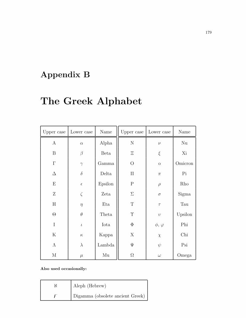
179
Appendix B
The Greek Alphabet
Upper case Lower case Name
A α Alpha
B β Beta
Γ γ Gamma
∆ δ Delta
E ǫ Epsilon
Z ζ Zeta
H η Eta
Θ θ Theta
I ι Iota
K κ Kappa
Λ λ Lambda
M µ Mu
Upper case Lower case Name
N ν Nu
Ξ ξ Xi
O o Omicron
Π π Pi
P ρ Rho
Σ σ Sigma
T τ Tau
Υ υ Upsilon
Φ φ, ϕ Phi
X χ Chi
Ψ ψ Psi
Ω ω Omega
Also used occasionally:
ℵ Aleph (Hebrew)
Digamma (obsolete ancient Greek)
180 QUADRIC SURFACES
Appendix C
Quadric Surfaces
A quadric surface is one defined by a quadratic equation of the variables (x, y, z), i.e an equation
of the form
ax2 + bxy + cxz + dy2 + eyz + fz2 + gx+ hy + jz + k = 0
The classification of the different forms of equation is beyond this course. Suffice to say that by
changing variables one can put the equation into one of 17 different standard forms, some of which
have no real solutions.
Six of standard forms occur very frequently in the notes as examples:
• The ellipsoid, ax2 + by2 + cz2 = 1
This includes the sphere and spheroids as special cases. If a = b = c then the surface is a
sphere. If a = b 6= c then it is a spheroid. If the spheroid is flattened (c > a) it is called
oblate, and if it is stretched (c < a) it is called prolate.
• The elliptic paraboloid, z = ax2 + by2
This includes the paraboloid of revolution as a special case
• The hyperbolic paraboloid or saddle, z = ax2 − by2
• The hyperboloid of one sheet, z2 = ax2 + by2 − c
• The hyperboloid of two sheets, z2 = ax2 − by2 + c
• The elliptic cone, z2 = ax2 + by2. This is a cone where the cross sections are ellipses.
This includes the standard circular cone as a special case.
• The elliptic cylinder, ax2 + by2 = 1. This is a cylinder where the cross section is an ellipse.
This includes the circular cylinder.
One can also obtain parabolic and hyperbolic cylinders, intersecting and parallel planes as well as
various degenerate solutions.
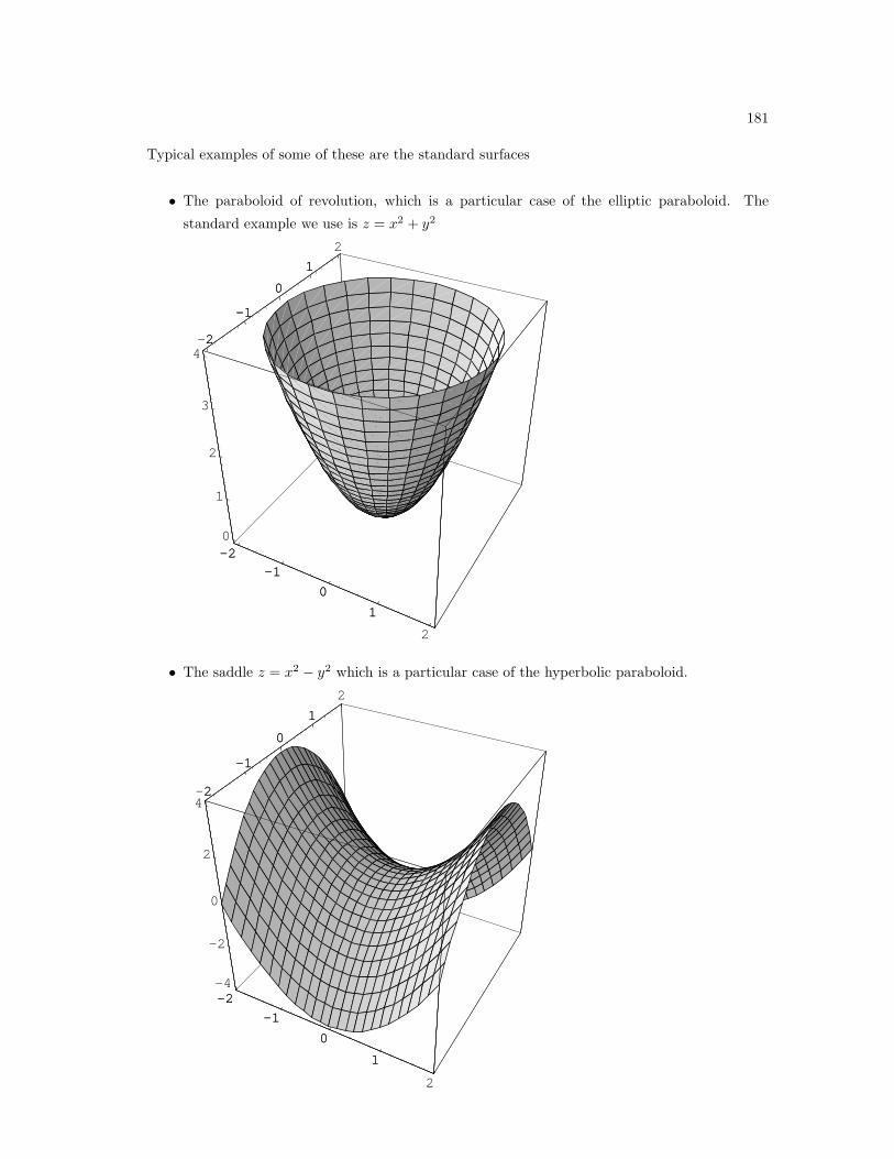
181
Typical examples of some of these are the standard surfaces
• The paraboloid of revolution, which is a particular case of the elliptic paraboloid. The
standard example we use is z = x2 + y2
-2
-1
0
1
2
-2
-1
0
1
2
0
1
2
3
4
-2
-1
0
1
2
-2
-1
0
1
2
• The saddle z = x2 − y2 which is a particular case of the hyperbolic paraboloid.
-2
-1
0
1
2
-2
-1
0
1
2
-4
-2
0
2
4
-2
-1
0
1
-2
-1
0
1
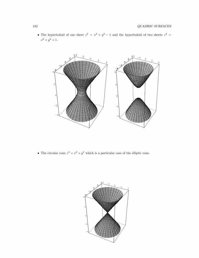
182 QUADRIC SURFACES
• The hyperboloid of one sheet z2 = x2 + y2 − 1 and the hyperboloid of two sheets z2 =
x2 + y2 + 1.
-4-2
02
4
-4
-2
0
24
-4
-2
0
2
4-4
-2
0
24 -4
-20
24
-4-2
02
4
-4
-2
0
2
4
-4-2
02
4
• The circular cone z2 = x2 + y2 which is a particular case of the elliptic cone.
-4-2
02
4
-4
-2
0
24
-4
-2
0
2
4-4
-2
0
24
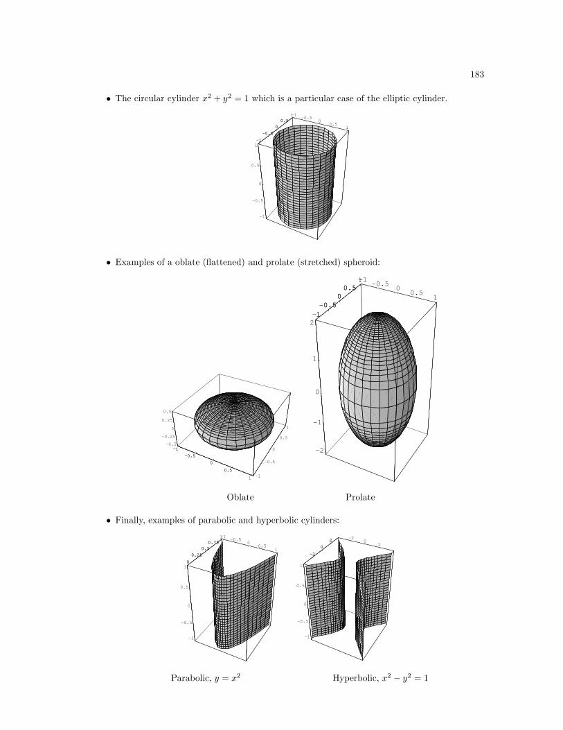
183
• The circular cylinder x2 + y2 = 1 which is a particular case of the elliptic cylinder.
-1-0.5
00.5
1
-1
-0.5
00.5
1
-1
-0.5
0
0.5
1-1
-0.5
00.5
1
• Examples of a oblate (flattened) and prolate (stretched) spheroid:
-1
-0.5
0
0.5
1 -1
-0.5
0
0.5
1
-0.5
-0.25
0
0.25
0.5
-1
-0.5
0
0.5
1
-1-0.5
00.5
1
-1-0.5
00.5
1
-2
-1
0
1
2-1-0.5
00.5
1
Oblate Prolate
• Finally, examples of parabolic and hyperbolic cylinders:
-1-0.5
00.5
1
0
0.25
0.50.75
1
-1
-0.5
0
0.5
10
0.25
0.50.75
1 -20
2
-2
0
2
-1
-0.5
0
0.5
1
-2
0
2
Parabolic, y = x2 Hyperbolic, x2 − y2 = 1
184 PROOFS OF THEOREMS
Appendix D
Proofs of theorems
D.1 Proof of Stokes’ Theorem, theorem 8.6.1
We need to prove∫ ∫
S
(∇× v) · n dσ =
∮
C
v · dr (8.13)
We can simplify the proof by considering each component of v separately. If we write
v(x, y, z) = v1(z, y, z)i+ v2(z, y, z)j+ v3(z, y, z)k
then we can consider three new vector fields
u1(x, y, z) = v1(x, y, z)i =
v1
0
0
, u2 = v2j =
0
v2
0
, u3 = v3k =
0
0
v3
,
and clearly v = u1 + u2 + u3, so that to prove Stokes’ theorem, all we need to do is prove it for
each of the vector fields ui, that is
∫ ∫
S
(∇× ui) · n dσ =
∮
C
ui · dr for i = 1, 2, 3
We will do the case i = 1, the others will clearly be true using the same method.
We will next assume that S is the graph of a function f(x, y) lying over the region Ω in the )x, y)-
plane. If S is not the graph of a function, we can split it into pieces which are graphs and combine
the result for each piece to arrive at the theorem.
Now we consider u1 = v1(x, y, z)i
∇× u1 =∂ v1∂ z
j− ∂ v1∂ y
k
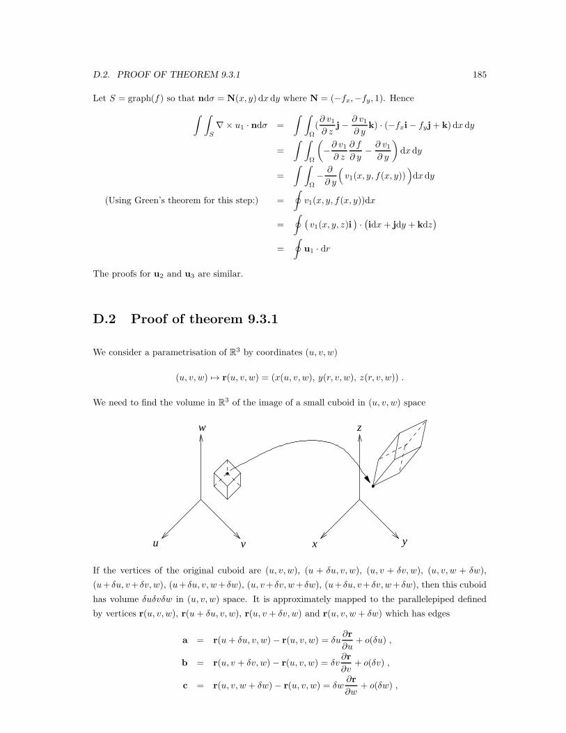
D.2. PROOF OF THEOREM 9.3.1 185
Let S = graph(f) so that ndσ = N(x, y) dx dy where N = (−fx,−fy, 1). Hence∫ ∫
S
∇× u1 · ndσ =
∫ ∫
Ω
(∂ v1∂ z
j− ∂ v1∂ y
k) · (−fxi− fyj+ k) dx dy
=
∫ ∫
Ω
(
−∂ v1∂ z
∂ f
∂ y− ∂ v1
∂ y
)
dxdy
=
∫ ∫
Ω
− ∂
∂ y
(
v1(x, y, f(x, y)))
dxdy
(Using Green’s theorem for this step:) =
∮
v1(x, y, f(x, y))dx
=
∮(v1(x, y, z)i
)·(idx+ jdy + kdz
)
=
∮
u1 · dr
The proofs for u2 and u3 are similar.
D.2 Proof of theorem 9.3.1
We consider a parametrisation of R3 by coordinates (u, v, w)
(u, v, w) 7→ r(u, v, w) = (x(u, v, w), y(r, v, w), z(r, v, w)) .
We need to find the volume in R3 of the image of a small cuboid in (u, v, w) space
w
vu x y
z
If the vertices of the original cuboid are (u, v, w), (u + δu, v, w), (u, v + δv, w), (u, v, w + δw),
(u+ δu, v+ δv, w), (u+ δu, v, w+ δw), (u, v+ δv, w+ δw), (u+ δu, v+ δv, w+ δw), then this cuboid
has volume δuδvδw in (u, v, w) space. It is approximately mapped to the parallelepiped defined
by vertices r(u, v, w), r(u+ δu, v, w), r(u, v + δv, w) and r(u, v, w + δw) which has edges
a = r(u+ δu, v, w)− r(u, v, w) = δu∂r
∂u+ o(δu) ,
b = r(u, v + δv, w)− r(u, v, w) = δv∂r
∂v+ o(δv) ,
c = r(u, v, w + δw) − r(u, v, w) = δw∂r
∂w+ o(δw) ,
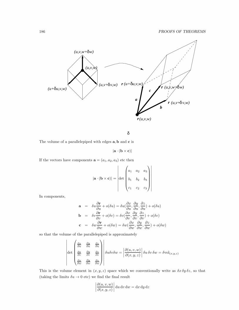
186 PROOFS OF THEOREMS
(u,v,w)
a
b
c
δ
δ
δδ r
rδ
δ
r δ
(u,v,w)r
(u,v,w+ w)
(u+ u,v,w)(u,v+ v,w) (u+ u,v,w)
(u,v,w+ w)
(u,v+ v,w)
The volume of a parallelepiped with edges a,b and c is
|a · (b× c)|
If the vectors have components a = (a1, a2, a3) etc then
|a · (b× c)| =
∣∣∣∣∣∣∣∣∣∣∣
det
a1 a2 a3
b1 b2 b3
c1 c2 c3
∣∣∣∣∣∣∣∣∣∣∣
In components,
a = δu∂r
∂u+ o(δu) = δu(
∂x
∂u,∂y
∂u,∂z
∂u) + o(δu)
b = δv∂r
∂v+ o(δv) = δv(
∂x
∂v,∂y
∂v,∂z
∂v) + o(δv)
c = δw∂r
∂w+ o(δw) = δw(
∂x
∂w,∂y
∂w,∂z
∂w) + o(δw)
so that the volume of the parallelepiped is approximately∣∣∣∣∣∣∣∣∣∣∣
det
∂x∂u
∂y∂u
∂z∂u
∂x∂v
∂y∂v
∂z∂v
∂x∂w
∂y∂w
∂z∂w
∣∣∣∣∣∣∣∣∣∣∣
δuδvδw =
∣∣∣∣
∂(u, v, w)
∂(x, y, z)
∣∣∣∣δu δv δw = δvol(x,y,z)
This is the volume element in (x, y, z) space which we conventionally write as δx δy δz, so that
(taking the limits δu→ 0 etc) we find the final result∣∣∣∣
∂(u, v, w)
∂(x, y, z)
∣∣∣∣du dv dw = dxdy dz
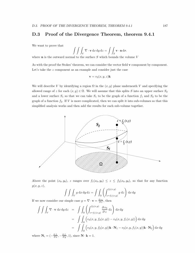
D.3. PROOF OF THE DIVERGENCE THEOREM, THEOREM 9.4.1 187
D.3 Proof of the Divergence Theorem, theorem 9.4.1
We want to prove that ∫ ∫ ∫
V
∇ · v dxdy dz =
∫ ∫
S
v · n dσ.
where n is the outward normal to the surface S which bounds the volume V
As with the proof the Stokes’ theorem, we can consider the vector field v component by component.
Let’s take the z component as an example and consider just the case
v = v3(x, y, z)k
We will describe V by identifying a region Ω in the (x, y) plane underneath V and specifying the
allowed range of z for each (x, y) ∈ Ω. We will assume that this splits S into an upper surface S2
and a lower surface S1 so that we can take S1 to be the graph of a function f1 and S2 to be the
graph of a function f2. If V is more complicated, then we can split it into sub-volumes so that this
simplified analysis works and then add the results for each sub-volume together.
S2
S1
Ω
z = f (x,y)
z = f (x,y)
2
1
Above the point (x0, y0), z ranges over f1(x0, y0) ≤ z ≤ f2(x0, y0), so that for any function
g(x, y, z),∫ ∫ ∫
V
g dx dy dz =
∫ ∫
Ω
(∫ f2(x,y)
z=f1(x,y)
g dz
)
dxdy
If we now consider our simple case g = ∇ · v = ∂ v3∂ z , then
∫ ∫ ∫
V
∇ · v dxdy dz =
∫ ∫
Ω
(∫ f2(x,y)
z=f1(x,y)
∂ v3∂ z
dz
)
dxdy
=
∫ ∫
Ω
(
v3(x, y, f2(x, y)) − v3(x, y, f1(x, y)))
dxdy
=
∫ ∫
Ω
(
v3(x, y, f2(x, y))k ·N1 − v3(x, y, f1(x, y))k ·N2
)
dx dy
where Ni = (−∂ fi∂ x ,−
∂ fi∂ y , 1), since N · k = 1.
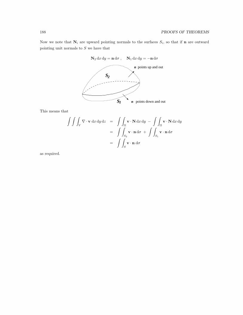
188 PROOFS OF THEOREMS
Now we note that Ni are upward pointing normals to the surfaces Si, so that if n are outward
pointing unit normals to S we have that
N2 dx dy = n dσ , N1 dx dy = −n dσ
S2
S1
n
n points down and out
points up and out
This means that∫ ∫ ∫
V
∇ · v dxdy dz =
∫ ∫
Ω
v ·N dxdy −∫ ∫
Ω
v ·N dxdy
=
∫ ∫
S2
v · n dσ +
∫ ∫
S1
v · n dσ
=
∫ ∫
S
v · n dσ
as required.