1

1.1 THE CONTROL SYSTEM

The control system is that means by which any quantity of interest in a machine, mechanismor other equipment is maintained or altered in accordance with a desired manner. Consider,for example, the driving system of an automobile. Speed of the automobile is a function of theposition of its accelerator. The desired speed can be maintained (or a desired change in speedcan be achieved) by controlling pressure on the accelerator pedal. This automobile drivingsystem (accelerator, carburettor and engine-vehicle) constitutes a control system. Figure 1.1shows the general diagrammatic representation of a typical control system. For the automobiledriving system the input (command) signal is the force on the accelerator pedal which throughlinkages causes the carburettor valve to open (close) so as to increase or decrease fuel (liquid form)flow to the engine bringing the engine-vehicle speed (controlled variable) to the desired value.

Accelerator pedal,linkages andcarburetter

Input (command)signal

ForceEngine-vehicle

Output (controlled)variable

Speed

Rate offuel flow

Fig. 1.1. The basic control system.

The diagrammatic representation of Fig. 1.1 is known as block diagram representationwherein each block represents an element, a plant, mechanism, device etc., whose inner detailsare not indicated. Each block has an input and output signal which are linked by a relationshipcharacterizing the block. It may be noted that the signal flow through the block is unidirectional.

�

�����������

2 A TEXTBOOK OF CONTROL SYSTEMS ENGINEERING

Closed-Loop Control

Let us reconsider the automobile driving system. The route, speed and acceleration of theautomobile are determined and controlled by the driver by observing traffic and road conditionsand by properly manipulating the accelerator, clutch, gear-lever, brakes and steering wheel,etc. Suppose the driver wants to maintain a speed of 50 km per hour (desired output). Heaccelerates the automobile to this speed with the help of the accelerator and then maintains itby holding the accelerator steady. No error in the speed of the automobile occurs so long asthere are no gradients or other disturbances along the road. The actual speed of the automobileis measured by the speedometer and indicated on its dial. The driver reads the speed dialvisually and compares the actual speed with the desired one mentally. If there is a deviation ofspeed from the desired speed, accordingly he takes the decision to increase or decrease thespeed. The decision is executed by change in pressure of his foot (through muscular power) onthe accelerator pedal.

These operations can be represented in a diagrammatic form as shown in Fig. 1.2. Incontrast to the sequence of events in Fig. 1.1, the events in the control sequence of Fig. 1.2follow a closed-loop, i.e., the information about the instantaneous state of the output is feedbackto the input and is used to modify it in such a manner as to achieve the desired output. It is onaccount of this basic difference that the system of Fig. 1.1 is called an open-loop system, whilethe system of Fig. 1.2 is called a closed-loop system.

Driver’s eyesand brain

Desiredspeed Leg

muscles

Accelerator pedal,linkages andcarburetter

Engine-vehicle

Visual link from speedometerSpeedometer

Outputspeed

Force

Rate offuel flow

Fig. 1.2. Schematic diagram of a manually controlled closed-loop system.

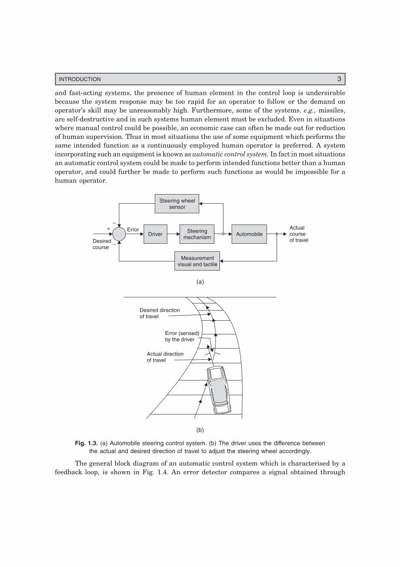
Let us investigate another control aspect of the above example of an automobile (enginevehicle) say its steering mechanism. A simple block diagram of an automobile steeringmechanism is shown in Fig. 1.3(a). The driver senses visually and by tactile means (bodymovement) the error between the actual and desired directions of the automobile as in Fig. 1.3(b).Additional information is available to the driver from the feel (sensing) of the steering wheelthrough his hand(s), these informations constitute the feedback signal(s) which are interpretedby driver’s brain, who then signals his hand to adjust the steering wheel accordingly. Thisagain is an example of a closed-loop system where human visual and tactile measurementsconstitute the feedback loop.

In fact unless human being(s) are not left out of in a control system study practically allcontrol systems are a sort of closed-loop system (with intelligent measurement and sensingloop or there may indeed by several such loops).

Systems of the type represented in Figs. 1.2 and 1.3 involve continuous manual controlby a human operator. These are classified as manually controlled systems. In many complex

INTRODUCTION 3

and fast-acting systems, the presence of human element in the control loop is undersirablebecause the system response may be too rapid for an operator to follow or the demand onoperator’s skill may be unreasonably high. Furthermore, some of the systems. e.g., missiles,are self-destructive and in such systems human element must be excluded. Even in situationswhere manual control could be possible, an economic case can often be made out for reductionof human supervision. Thus in most situations the use of some equipment which performs thesame intended function as a continuously employed human operator is preferred. A systemincorporating such an equipment is known as automatic control system. In fact in most situationsan automatic control system could be made to perform intended functions better than a humanoperator, and could further be made to perform such functions as would be impossible for ahuman operator.

Steeringmechanism

Driver Automobile

Steering wheelsensor

Measurementvisual and tactile

Error–

–

+

Desiredcourse

Actualcourseof travel

(a)

Error (sensed)by the driver

Desired directionof travel

Actual directionof travel

(b)

Fig. 1.3. (a) Automobile steering control system. (b) The driver uses the difference betweenthe actual and desired direction of travel to adjust the steering wheel accordingly.

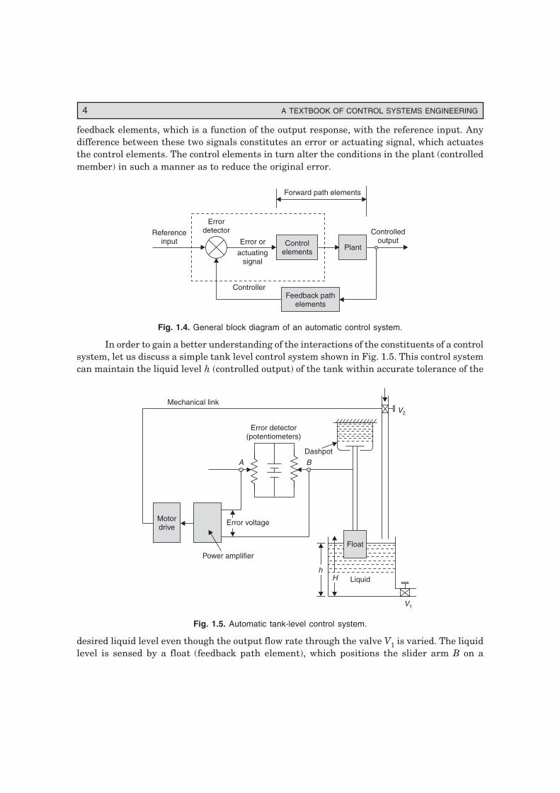
The general block diagram of an automatic control system which is characterised by afeedback loop, is shown in Fig. 1.4. An error detector compares a signal obtained through

4 A TEXTBOOK OF CONTROL SYSTEMS ENGINEERING

feedback elements, which is a function of the output response, with the reference input. Anydifference between these two signals constitutes an error or actuating signal, which actuatesthe control elements. The control elements in turn alter the conditions in the plant (controlledmember) in such a manner as to reduce the original error.

Controlelements

Error or

actuatingsignal

ErrordetectorReference

inputPlant

Feedback pathelements

Controlledoutput

Forward path elements

Controller

Fig. 1.4. General block diagram of an automatic control system.

In order to gain a better understanding of the interactions of the constituents of a controlsystem, let us discuss a simple tank level control system shown in Fig. 1.5. This control systemcan maintain the liquid level h (controlled output) of the tank within accurate tolerance of the

H Liquidh

V1

Error voltage

Power amplifier

Motordrive

A B

Error detector(potentiometers)

Dashpot

Mechanical linkV2

Float

Fig. 1.5. Automatic tank-level control system.

desired liquid level even though the output flow rate through the valve V1 is varied. The liquidlevel is sensed by a float (feedback path element), which positions the slider arm B on a

INTRODUCTION 5

potentiometer. The slider arm A of another potentiometer is positioned corresponding to thedesired liquid level H (the reference input). When the liquid level rises or falls, thepotentiometers (error detector) give an error voltage (error or actuating signal) proportional tothe change in liquid level. The error voltage actuates the motor through a power amplifier(control elements) which in turn conditions the plant (i.e., decreases or increases the openingof the valve V2) in order to restore the desired liquid level. Thus the control system automaticallyattempts to correct any deviation between the actual and desired liquid levels in the tank.

Open-Loop Control

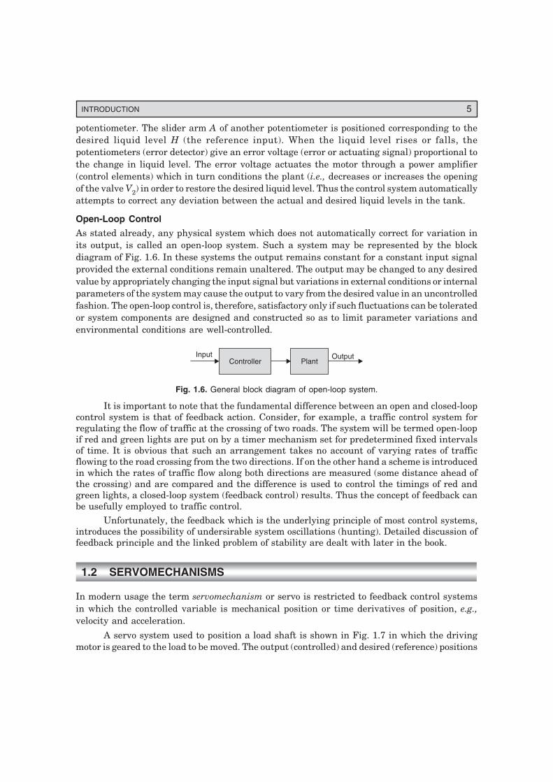
As stated already, any physical system which does not automatically correct for variation inits output, is called an open-loop system. Such a system may be represented by the blockdiagram of Fig. 1.6. In these systems the output remains constant for a constant input signalprovided the external conditions remain unaltered. The output may be changed to any desiredvalue by appropriately changing the input signal but variations in external conditions or internalparameters of the system may cause the output to vary from the desired value in an uncontrolledfashion. The open-loop control is, therefore, satisfactory only if such fluctuations can be toleratedor system components are designed and constructed so as to limit parameter variations andenvironmental conditions are well-controlled.

Controller PlantOutputInput

Fig. 1.6. General block diagram of open-loop system.

It is important to note that the fundamental difference between an open and closed-loopcontrol system is that of feedback action. Consider, for example, a traffic control system forregulating the flow of traffic at the crossing of two roads. The system will be termed open-loopif red and green lights are put on by a timer mechanism set for predetermined fixed intervalsof time. It is obvious that such an arrangement takes no account of varying rates of trafficflowing to the road crossing from the two directions. If on the other hand a scheme is introducedin which the rates of traffic flow along both directions are measured (some distance ahead ofthe crossing) and are compared and the difference is used to control the timings of red andgreen lights, a closed-loop system (feedback control) results. Thus the concept of feedback canbe usefully employed to traffic control.

Unfortunately, the feedback which is the underlying principle of most control systems,introduces the possibility of undersirable system oscillations (hunting). Detailed discussion offeedback principle and the linked problem of stability are dealt with later in the book.

1.2 SERVOMECHANISMS

In modern usage the term servomechanism or servo is restricted to feedback control systemsin which the controlled variable is mechanical position or time derivatives of position, e.g.,velocity and acceleration.

A servo system used to position a load shaft is shown in Fig. 1.7 in which the drivingmotor is geared to the load to be moved. The output (controlled) and desired (reference) positions

6 A TEXTBOOK OF CONTROL SYSTEMS ENGINEERING

qC and qR respectively are measured and compared by a potentiometer pair whose outputvoltage vE is proportional to the error in angular position qE = qR – qC. The voltage vE = KPqE isamplified and is used to control the field current (excitation) of a dc generator which suppliesthe armature voltage to the drive motor.

To understand the operation of the system assume KP = 100 volts/rad and let the outputshaft position be 0.5 rad. Corresponding to this condition, the slider arm B has a voltage of +50volts. Let the slider arm A be also set at +50 volts. This gives zero actuating signal (vE = 0).Thus the motor has zero output torque so that the load stays stationary at 0.5 rad.

Assume now that the new desired load position is 0.6 rad. To achieve this, the arm A isplaced at +60 volts position, while the arm B remains instantaneously at +50 volts position.This creates an actuating signal of +10 volts, which is a measure of lack of correspondencebetween the actual load position and the commanded position. The actuating signal is amplifiedand fed to the servo motor which in turn generates an output torque which repositions theload. The system comes to a standstill only when the actuating signal becomes zero, i.e., thearm B and the load reach the position corresponding to 0.6 rad (+60 volts position).

Consider now that a load torque TL is applied at the output as indicated in Fig. 1.7. Thiswill require a steady value of error voltage vE which acting through the amplifier, generator,motor and gears will counterbalance the load torque. This would mean that a steady error willexist between the input and output angles. This is unlike the case when there is no load torqueand consequently the angle error is zero. In control terminology, such loads are known as loaddisturbances and system has to be designed to keep the error to these disturbances withinspecified limits.

AB

vEAmplifier

Constant

MotorGenerator

Load

TL

Gears

100volts

Feedbackpotentiometer

Inputpotentiometer

�C�R

Current

Fig. 1.7. A position control system.

By opening the feedback loop i.e., disconnecting the potentiometer B, the reader caneasily verify that any operator acting as part of feedback loop will find it very difficult to adjustqC to a desired value and to be able to maintain it. This further demonstrates the power of anegative feedback (hardware) loop.

INTRODUCTION 7

The position control systems have innumerable applications, namely, machine toolposition control, constant-tension control of sheet rolls in paper mills, control of sheet metalthickness in hot rolling mills, radar tracking systems, missile guidance systems, inertialguidance, roll stabilization of ships, etc. Some of these applications will be discussed in thisbook.

1.3 HISTORY AND DEVELOPMENT OF AUTOMATIC CONTROL

It is instructive to trace brief historical development of automatic control. Automatic controlsystems did not appear until the middle of eighteenth century. The first automatic controlsystem, the fly-ball governor, to control the speed of steam engines, was invented by JamesWatt in 1770. This device was usually prone to hunting. It was about hundred years later thatMaxwell analyzed the dynamics of the fly-ball governor.

The schematic diagram of a speed control system using a fly-ball governor is shown inFig. 1.8. The governor is directly geared to the output shaft so that the speed of the fly-balls isproportional to the output speed of the engine. The position of the throttle lever sets the desiredspeed. The lever pivoted as shown in Fig. 1.8 transmits the centrifugal force from the fly-ballsto the bottom of the lower seat of the spring. Under steady conditions, the centrifugal force ofthe fly-balls balances the spring force* and the opening of flow control valve is just sufficient tomaintain the engine speed at the desired value.

x

Desired speed

Throttlelever

Fly-ball

LeverPivot

Flow control valve

Fuel flow toengine

Fig. 1.8. Speed control system.

* The gravitational forces are normally negligible compared to the centrifugal force.

8 A TEXTBOOK OF CONTROL SYSTEMS ENGINEERING

If the engine speed drops below the desired value, the centrifugal force of the fly-ballsdecreases, thus decreasing the force exerted on the bottom of the spring, causing x to movedownward. By lever action, this results in wider opening of the control valve and hence morefuel supply which increases the speed of the engine until equilibrium is restored. If the speedincreases, the reverse action takes place.

The change in desired engine speed can be achieved by adjusting the setting of throttlelever. For a higher speed setting, the throttle lever is moved up which in turn causes x to movedownward resulting in wider opening of the fuel control valve with consequent increase ofspeed. The lower speed setting is achieved by reverse action.

The importance of positioning heavy masses like ships and guns quickly and preciselywas realized during the World War I. In early 1920, Minorsky performed the classic work onthe automatic steering of ships and positioning of guns on the shipboards.

A date of significance in automatic control systems in that of Hazen’s work in 1934. Hiswork may possibly be considered as a first struggling attempt to develop some general theoryfor servomechanisms. The word ‘servo’ has originated with him.

Prior to 1940 automatic control theory was not much developed and for most cases thedesign of control systems was indeed an art. During the decade of 1940’s, mathematical andanalytical methods were developed and practised and control engineering was established asan engineering discipline in its own rights. During the World War II it became necessary todesign and construct automatic aeroplane pilots, gun positioning systems, radar trackingsystems and other military equipments based on feedback control principle. This gave a greatimpetus to the automatic control theory.

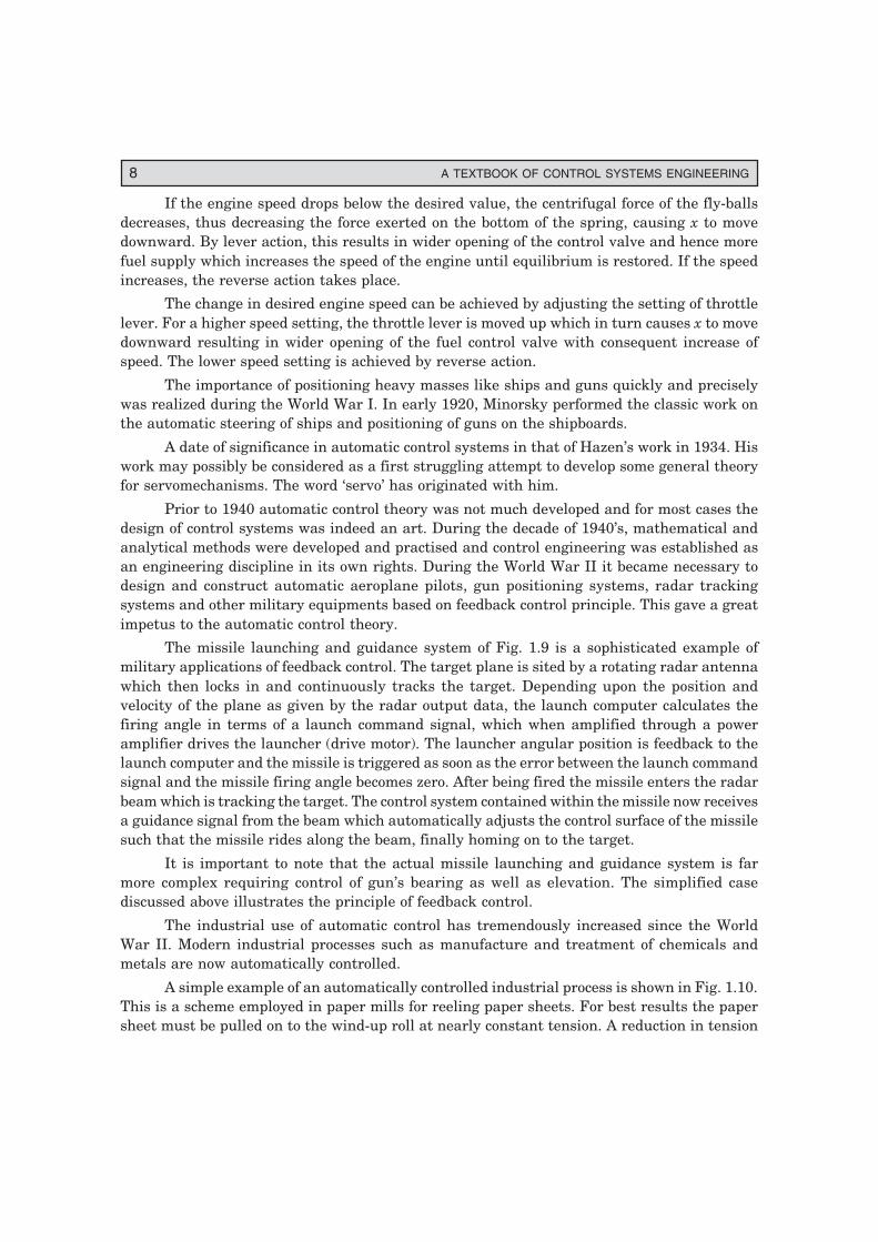
The missile launching and guidance system of Fig. 1.9 is a sophisticated example ofmilitary applications of feedback control. The target plane is sited by a rotating radar antennawhich then locks in and continuously tracks the target. Depending upon the position andvelocity of the plane as given by the radar output data, the launch computer calculates thefiring angle in terms of a launch command signal, which when amplified through a poweramplifier drives the launcher (drive motor). The launcher angular position is feedback to thelaunch computer and the missile is triggered as soon as the error between the launch commandsignal and the missile firing angle becomes zero. After being fired the missile enters the radarbeam which is tracking the target. The control system contained within the missile now receivesa guidance signal from the beam which automatically adjusts the control surface of the missilesuch that the missile rides along the beam, finally homing on to the target.

It is important to note that the actual missile launching and guidance system is farmore complex requiring control of gun’s bearing as well as elevation. The simplified casediscussed above illustrates the principle of feedback control.

The industrial use of automatic control has tremendously increased since the WorldWar II. Modern industrial processes such as manufacture and treatment of chemicals andmetals are now automatically controlled.

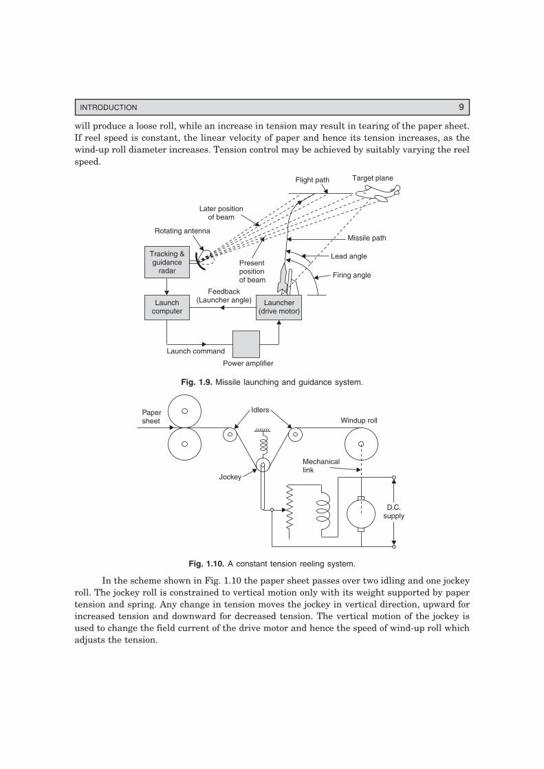
A simple example of an automatically controlled industrial process is shown in Fig. 1.10.This is a scheme employed in paper mills for reeling paper sheets. For best results the papersheet must be pulled on to the wind-up roll at nearly constant tension. A reduction in tension

INTRODUCTION 9

will produce a loose roll, while an increase in tension may result in tearing of the paper sheet.If reel speed is constant, the linear velocity of paper and hence its tension increases, as thewind-up roll diameter increases. Tension control may be achieved by suitably varying the reelspeed.

Tracking &guidance

radar

Launchcomputer

Launcher(drive motor)

Feedback(Launcher angle)

Launch command

Power amplifier

Presentpositionof beam

Later positionof beam

Rotating antenna

Flight path Target plane

Missile path

Lead angle

Firing angle

Fig. 1.9. Missile launching and guidance system.

Mechanicallink

D.C.supply

IdlersPapersheet

Jockey

Windup roll

Fig. 1.10. A constant tension reeling system.

In the scheme shown in Fig. 1.10 the paper sheet passes over two idling and one jockeyroll. The jockey roll is constrained to vertical motion only with its weight supported by papertension and spring. Any change in tension moves the jockey in vertical direction, upward forincreased tension and downward for decreased tension. The vertical motion of the jockey isused to change the field current of the drive motor and hence the speed of wind-up roll whichadjusts the tension.

10 A TEXTBOOK OF CONTROL SYSTEMS ENGINEERING

Control engineering has enjoyed tremendous growth during the years since 1955.Particularly with the advent of analog and digital computers and with the perfection achievedin computer field, highly sophisticated control schemes have been devised and implemented.Furthermore, computers have opened up vast vistas for applying control concepts to non-engineering fields like business and management. On the technological front fully automatedcomputer control schemes have been introduced for electric utilities and many complexindustrial processes with several interacting variables particularly in the chemical andmetallurgical processes.

A glorious future lies ahead for automation wherein computer control can run ourindustries and produce our consumer goods provided we can tackle with equal vigour andsuccess the socio-economic and resource depletion problems associated with such sophisticateddegree of automation.

1.4 DIGITAL COMPUTER CONTROL

In some of the examples of control systems of high level of complexity (robot manipulator ofFig. 1.8 and missile launching and guidance system of Fig. 1.9) it is seen that such controlsystems need a digital computer as a control element to digitally process a number of inputsignals to generate a number of control signals so as to manipulate several plant variables. Inthese control systems signals in certain parts of the plant are in analog form i.e., continuousfunctions of the time variable, while the control computer handles data only in digital (ordiscrete) form. This requires signal discretization and analog-to-digital interfacing in form ofA/D and D/A converters.

To begin with we will consider a simple form the digital control system knows as sampled-data control system. The block diagram of such a system with single feedback loop is illustratedin Fig. 1.11 wherein the sampler samples the error signal e(t) every T seconds. The sampler isan electronic switch whose output is the discritized version of the analog error signal and is atrain of pulses of the sampling frequency with the strength of each pulse being that the errorsignal at the beginning of the sampling period. The sampled signal is passed through a datahold and is then filtered by a digital filter in accordance with the control algorithm. The smoothedout control signal u(t) is then used to manipulate the plant.

Data holddigital filter

e ts( )Plant

T

u t( ) c t( )

Output+

–

e t( )r t( )

CommandPulse train

Fig. 1.11. Block diagram of a sampled-data control system.

It is seen above that computer control is needed in large and complex control schemesdealing with a number of input, output variables and feedback channels. This is borne out bythe example of Fig. 1.9. Such systems are referred to as multivariable control systems whosegeneral block diagram is shown in Fig. 1.12.

INTRODUCTION 11

ControllerInput

variablesOutput

variables

Feedbackelements

Plant

Fig. 1.12. General block diagram of a multivariable control system.

Where a few variable are to be controlled with a limited number of commands and thecontrol algorithm is of moderate complexity and the plant process to be controlled is at a givenphysical location, a general purpose computer chip, the microprocessor (mP) is commonlyemployed. Such systems are known as mP-based control systems. Of course at the input/outputinterfacing A/D and D/A converter chips would be needed.

For large systems a central computer is employed for simultaneous control of severalsubsystems wherein certain hierarchies are maintained keeping in view the overall systemobjectives. Additional functions like supervisory control, fault recording, data logging etc, alsobecome possible. We shall advance two examples of central computer control.

Automatic Aircraft Landing System

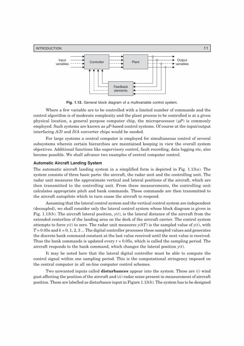
The automatic aircraft landing system in a simplified form is depicted in Fig. 1.13(a). Thesystem consists of three basic parts: the aircraft, the radar unit and the controlling unit. Theradar unit measures the approximate vertical and lateral positions of the aircraft, which arethen transmitted to the controlling unit. From these measurements, the controlling unitcalculates appropriate pitch and bank commands. These commands are then transmitted tothe aircraft autopilots which in turn cause the aircraft to respond.

Assuming that the lateral control system and the vertical control system are independent(decoupled), we shall consider only the lateral control system whose block diagram is given inFig. 1.13(b). The aircraft lateral position, y(t), is the lateral distance of the aircraft from theextended centerline of the landing area on the deck of the aircraft carrier. The control systemattempts to force y(t) to zero. The radar unit measures y(kT) is the sampled value of y(t), withT = 0.05s and k = 0, 1, 2, 3 ... The digital controller processes these sampled values and generatesthe discrete bank command constant at the last value received until the next value is received.Thus the bank commands is updated every t = 0.05s, which is called the sampling period. Theaircraft responds to the bank command, which changes the lateral position y(t).

It may be noted here that the lateral digital controller must be able to compute thecontrol signal within one sampling period. This is the computational stringency imposed onthe central computer in all on-line computer control schemes.

Two unwanted inputs called disturbances appear into the system. These are (i) windgust affecting the position of the aircraft and (ii) radar noise present in measurement of aircraftposition. These are labelled as disturbance input in Figure 1.13(b). The system has to be designed

12 A TEXTBOOK OF CONTROL SYSTEMS ENGINEERING

Transmitter

Controllingunit

Bankcommand

Pitchcommand

Radarunit

Lateralposition

Verticalposition

Aircraft

(a) Schematic

Lateraldigital

controller

Desiredposition

Aircraftlateralsystem

Datahold

y t( )

Aircraftposition

�( )t

Bankcommand

Radarnoise

++

T

y kT( )

Radar

w t( ), noise

(b) Lateral landing system.

Fig. 1.13. Automatic aircraft landing system.

to mitigate the effects of disturbance input so that the aircraft lands within acceptable limitsof lateral accuracy.

INTRODUCTION 13

Rocket Autopilot System

As another illustration of computer control, let us discuss an autopilot system which steers arocket vehicle in response to radioed command. Figure 1.14 shows a simplified block diagramrepresentation of the system.

The state of motion of the vehicle (velocity, acceleration) is fed to the control computerby means of motion sensors (gyros, accelerometers). A position pick-off feeds the computerwith the information about rocket engine angle displacement and hence the direction in whichthe vehicle is heading. In response to heading-commands from the ground, the computergenerates a signal which controls the hydraulic actuator and in turn moves the engine.

Radioreceiver

Radio command signal(from ground station)

Digitalcoded input

Digitalcomputer

Digital toanalog

converter

Hydraulicactuator

Rocketengine

Vehicledynamics

Controlsignal

Engine angledisplacement

Vehiclemotions

Position pick-off

Gyros

Accelerometer

Analogto

digitalconverter

Fig. 1.14. A typical autopilot system.

1.5 APPLICATION OF CONTROL THEORY IN NON-ENGINEERING FIELDS

We have considered in previous sections a number of applications which highlight thepotentialities of automatic control to handle various engineering problems. Although controltheory originally evolved as an engineering discipline, due to universality of the principlesinvolved it is no longer restricted to engineering confines in the present state of art. In thefollowing paragraphs we shall discuss some examples of control theory as applied to fields likeeconomics, sociology and biology.

Consider an economic inflation problem which is evidenced by continually rising prices.A model of the vicious price-wage inflationary cycle, assuming simple relationship betweenwages, product costs and cost of living is shown in Fig 1.15. The economic system depicted inthis figure is found to be a positive feedback system.

14 A TEXTBOOK OF CONTROL SYSTEMS ENGINEERING

K1

Industry

Presentwages

K2

Productcost

Cost ofliving

+

Initialwages

Dissatisfactionfactor dWage increment

+

Fig. 1.15. Economic inflation dynamics.

To introduce yet another example of non-engineering application of control principles,let us discuss the dynamics of epidemics in human beings and animals. A normal healthycommunity has a certain rate of daily contracts C. When an epidemic disease affects thiscommunity the social pattern is altered as shown in Fig. 1.16. The factor K1 contains the

Infectiouscontacts

Diseaseproducing contacts

+–

Rate of dailycontacts C

K1

K2

Fig. 1.16. Block diagram representation of epidemic dynamics.

statistical fraction of infectious contacts that actually produce the disease, while the factor K2accounts for the isolation of the sick people and medical immunization. Since the isolation andimmunization reduce the infectious contacts, the system has a negative feedback loop.

In medical field, control theory has wide applications, such as temperature regulation,neurological, respiratory and cardiovascular controls. A simple example is the automaticanaesthetic control. The degree of anaesthesia of a patient undergoing operation can bemeasured from encephalograms. Using control principles anaesthetic control can be madecompletely automatic, thereby freeing the anaesthetist from observing constantly the generalcondition of the patient and making manual adjustments.

The examples cited above are somewhat over-simplified and are introduced merely toillustrate the universality of control principles. More complex and complete feedback modelsin various non-engineering fields are now available. This area of control is under rapiddevelopment and has a promising future.

1.6 THE CONTROL PROBLEM

In the above account the field of control systems has been surveyed with a wide variety ofillustrative examples including those of some nonphysical systems. The basic block diagram ofa control system given in Fig. 1.3 is reproduced in Fig. 1.17 wherein certain alternative blockand signal nomenclature are introduced.

INTRODUCTION 15

Controlelements

(controller)

Error( )e t Plant

(process)u t( )

Controlledoutput ( )c t

+–

Commandinput ( )r t

Feedbackelements

Comparator

Disturbanceinput

Noise

b t( )

Fig. 1.17. The basic control loop.

Further the figure also indicates the presence of the disturbance input (load disturbance)in the plant and noise input in feedback element (noise enters in the measurement process;see example of automatic aircraft landing system in Fig. 1.14). This basic control loop withnegative feedback responds to reduce the error between the command input (desired output)and the controlled output.

Further as we shall see in later chapters that negative feedback has several benefitslike reduction in effects of disturbances input, plant nonlinearities and changes in plantparameters. A multivariable control system with several feedback loops essentially follows thesame logic. In some mechanical systems and chemical processes a certain signal also is directlyinput to the controller elements particularly to counter the effect of load disturbance (notshown in the figure).

Generally, a controller (or a filter) is required to process the error signal such that theoverall system statisfies certain criteria specifications. Some of these criteria are:

1. Reduction in effect of disturbance signal.

2. Reduction in steady-state errors.

3. Transient response and frequency response performance.

4. Sensitivity to parameter changes.

Solving the control problem in the light of the above criteria will generally involvefollowing steps:

1. Choice of feedback sensor(s) to get a measure of the controlled output.

2. Choice of actuator to drive (manipulate) the plant like opening or closing a valve,adjusting the excitation or armature voltage of a motor.

3. Developing mathematical models of plant, sensor and actuator.

4. Controller design based on models developed in step 3 and the specified criteria.

5. Simulating system performance and fine tuning.

6. Iterate the above steps, if necessary.

7. Building the system or its prototype and testing.

The criteria and steps involved in system design and implementation and tools of analysisneeded of this, form the subject matter of the later chapters.