Author : Sh. Dharmender Kumar Vetter : Dr. Manoj Dhun

Lesson No. : 01 Lesson Name: Introduction

Objective : To understand networking concepts, connection oriented and

connection less communication, network topologies, concept of LAN, MAN, WAN ,lastly and Analysis & comparison of OSI and TCP/IP reference model for data communication.

1.1 Introduction 1.1.1 What is Network

1.1.2 Elementary Terminology 1.1.3 Applications and uses of Network

1.2 History (Development) Networking 1.3 Network Topology

1.3.1 Star Topology 1.3.2 Bus Topology 1.3.3 Ring Topology 1.3.4 Tree Topology 1.3.5 Hybrid Topology

1.4 Network Hardware 1.4.1 LAN 1.4.2 MAN 1.4.3 WAN 1.4.4 Wireless Network 1.4.5 Home Network 1.4.6 Internetwork

1.5 Network Software 1.5.1 Protocol Hierarchies 1.5.2 Connection Oriented and Connectionless services 1.5.3 Service Primitives

1.6 OSI Reference Model 1.7 TCP/IP Reference Model 1.8 Comparison of TCP/IP and OSI Reference Model 1.9 Critique of OSI Reference model and TCP/IP reference

model 1.10 Summary 1.11 Self Assessment Questions

1.1 INTRODUCTION

Earlier, computer networks consisted of mainframes in an enclosure. Input

was in the form of punch cards read by card readers and output was in the form of

printed results via local printers. Local terminals were mostly used for control and

programming input. All processing was on a batch basis, rather than being

interactive. In other words, the input was transmitted in a batch from a card reader

over a short circuit to the processor, the processor processed the program in a batch

and the output to the printer was in a batch. The first true mainframe was the IBM

360, introduced in 1964. Over time, input to the mainframe was extended to

multiple users at dumb terminals that connected to ports on the mainframe through

terminal controllers, or cluster controllers.

In parallel to the development of data networking, the computers began

to change. Computers became more powerful as processor speeds increased

with the development of faster microprocessors on silicon chips. Memory

became more available as chip technology and hard drive technology

improved. Additionally, computers became smaller and less expensive, to the

point that the typical desktop PC is equivalent to an early mainframe that

would have filled a moderate-size office building. As a result, all of this

computing power and storage capability on all of these desktops would lead to

a need to network those devices within the workplace. It has been estimated

that majority of data transfer is confined to the workplace, while only small

percentage travels to remote places. Therefore, it is clear that PC users need to

share access to hosts, databases, printers, etc. LANs provide a solution to that

requirement.

Robert M. Metcalfe and his associates at the Xerox Palo Alto Research

Center (Xerox PARC) first conceived LAN technology. Later on, Xerox

commercialized the technology and named it The Xerox Wire. When Digital

Equipment Corporation (DEC), Intel and Xerox corporate to standardize the

technology in 1979, they named it to Ethernet. Ethernet quickly became a de facto

standard. Ethernet and LANs were officially recognized when the IEEE established

Project 802 at the request of members. In the end of 1982, the first standard was

published and circulated. Ethernet, clearly, is still the most popular LAN standard.

1.1.1 What is Network ?

Tenenbaum defines a network as an interconnected collection of autonomous

computers. Two computers are said to be interconnected if they are capable of

exchanging information. Central to this definition is the fact that the computers are

autonomous. This means that no computer on the network can start, stop, or control

another.

Advantages

Many organizations. already have a substantial number of computers, often

located far apart. For example, a company .with many offices may have a computer

at each location to keep track of customer orders, monitor sales, and do the local

payroll. Previously, each of these computers may have worked in isolation from

others but at some point, management decided to connect them together information

about entire company. In general we can refer to it as.

(I) RESOURCE SHARING. The aim is to make all programs, data and peripherals

available to anyone on the network irrespective of the physical location of the

resources and the user.

(ii) RELIABILITY. A file can have copies on two or three different machines, so if

one of . them is unavailable (hardware crash), the other copies could be used. For

military, banking, air reservation and many other applications it is of great

importance.

(iii) COST FACTOR. Personal computers have better price/performance ratio than

micro computers. So it is better to have PC's, one per user, with data stored on one

shared file server machine.

(iv) COMMUNICATION MEDIUM. Using a network, it is possible for managers,

working far apart, to prepare financial report of the company. The changes at one

end can be immediately noticed at another and hence it speeds up co-operation

among them.

1.1.2 ELEMENTARY TERMINOLOGY OF NETWORKS

It is some time to learn about the components/terms mostly used in

networking. Whenever we talk about a network it includes. the hardware and the

software that make up the network. Now let us have a look at some typical hardware

components of network.

Nodes (Workstations)

The term nodes refers to the computers that are attached to a network and are

seeking to share the resources of the network. Of course, if there were no nodes

(also called workstations), there would be no network at all.

A computer becomes a workstation of a network as soon as it is attached to a

network.

Server

Def:. A computer that facilitates "the sharing of data" software" and hardware -

resources (e.g. "printers" modems etc,) on the network" is termed as a SERVER.

On small networks, sometimes, all the shareable stuff (like files, data,

software etc.) is stored on the server. A network can have more than one server also.

Each server has a unique name on the network and all users of network identify the

server by its unique name. Servers can be of two types: non-dedicated and dedicated

servers.

Non-dedicated Servers:. On small networks, a workstation that can double

up as a server, is known as non-dedicated server since it is not completely dedicated

to the cause of serving. Such servers can facilitate the resource-sharing among

workstations on a proportionately smaller scale. Since one computer works as a

workstation as well as a server, it is .slower and requires. more memory. The (small)

networks using such a server are known as peer-to-peer networks.

Dedicated Servers:. On bigger network installations, there is a computer

reserved for server's job and its only job is to help workstations access data,

software and hardware resources. It does not double-up as a workstation and such a

server is known as dedicated server. The networks using such a server are known as

master-slave networks.

On a network, there may be several servers that allow workstations to share

specific resources. For example, there may be a server exc1usivelyfor serving files-

related requests like storing files, deciding about their access privileges and

regulating the amount of space allowed for each user. This server is known as file

server. Similarly, there may be printer server and modem server. The printer server

takes care of the printing requirements of a number of workstations and the modem

server helps a group of network users use a modem to transmit long distance

messages.

Network Interface Unit (NIU)

Def: A NETWORK INTERFACE UNIT is an interpreter that helps to establish

communication between the server and workstations.

A standalone computer (a computer that is not attached to a network) lives in

its own world and carries out its tasks with its own inbuilt resources. But as soon as

it becomes a workstation, it needs an interface to help establish a connection with

the network because without this, the workstations will not be able to share network

resources.

The network-interface-unit is a device that is attached to each of the

workstations and the server, and helps the workstation to establish the all-important

connection with the network. Each network-interface-unit that is attached to a

workstation has a unique number identifying it which is known as the node address.

The NIU is also called Terminal Access Point (TAP). Different manufacturers have

different names for the interface.

Computer networks can be used for numerous services, both for companies

and for individuals. For companies, networks of personal computers using shared

servers often provide access to corporate information. Typically they follow the

client-server model, with client workstations on employee desktops accessing

powerful servers in the machine room. For individuals, networks offer access to a

variety of information and entertainment resources. Individuals often access the

Internet by calling up an ISP using a modem, although increasingly many people

have a fixed connection at home. An up-and-coming area is wireless networking

with new application such as mobile e-mail access and m-commerce.

1.1.3 Applications & Uses of Networks

In the short time they have been around, data communication networks have

become an indispensable part of business, industry, and entertainment. Some of the

network applications in different fields are the following:

• Marketing and sales. Computer networks are used extensively in both

marketing and sales organizations. Marketing professionals use them to collect,

exchange, and analyze data relating to customer needs and product development

cycles. Sales applications include teleshopping, which uses order-entry computers or

telephones connected to an order-processing network, and on-line reservation

services for hotels, airlines, and so on.

• Financial services. Today's financial services are totally dependent on

computer networks. Applications include credit history searches, foreign exchange

and investment services, and electronic funds transfer (EFT), which allows a user, to

transfer money without going into a bank (an automated teller machine is a kind of

electronic funds transfer; automatic paycheck deposit is another).

• Manufacturing. Computer networks are used today in, many aspects of

manufacturing, including the manufacturing process itself. Two applications that use

networks to provide essential services are computer-assisted design (CAD) and

computer-assisted manufacturing (CAM), both of which allow multiple users to

work on a project simultaneously.

• Electronic messaging: Probably the most widely used network application

is electronic mail (e-mail).

• Directory services: Directory services allow lists of files to be stored in a

central location to speed worldwide search operations.

• Information services: Network information services include bulletin boards

and data banks. A World Wide Web site offering the technical specifications for a

new product is an information service.

• Electronic data interchange (EDI): EDI allows business information

(including documents such as purchase orders and invoices) to be transferred

without using paper.

• Teleconferencing: Teleconferencing allows conferences to occur without the

participants being in the same place. Applications include simple text conferencing

(where participants communicate through their keyboards and computer monitors).

voice conferencing (where participants at a number of locations communicate

simultaneously over the phone) and video conferencing (where participants can see

as well as talk to one another).

• Cellular telephone: In the past two parties wishing to use the services of the

telephone company had to be linked by a fixed physical connection. Today's cellular

networks make it possible to maintain wireless phone connections even while trav-

eling over large distances.

• Cable television: Future services provided by cable television networks may

include video on request, as well as the same information, financial, and commu-

nications services currently provided by the telephone companies and computer

networks.

1.2 History (Development) of Computer Networks

Each of the past three centuries has been dominated by a single technology.

The 18th century was the era of the great mechanical systems accompanying the

Industrial Revolution. The 19th century was the age' of the steam engine. During the

20th century, the key technology was information gathering, processing, and

distribution. Among other developments, we saw the installation of worldwide

telephone networks, the invention of radio and television, the birth and unprece-

dented growth of the computer industry, and the launching of communication

satellites.

As a result of rapid technological progress, these areas are rapidly converging

and the differences between collecting, transporting, storing, and processing infor-

mation are quickly disappearing. Organizations with hundreds of offices spread over

a wide geographical area routinely expect to be able to examine the current status of

even their most remote output at the push of a button. As our ability together,

process and distribute information grows, the demand forever more sophisticated

information processing grows even faster.

Although the computer industry is still young compared to other industries

(e.g., automobiles and air transportation), computers have made spectacular progress

in a short time. During the first two decades of their existence, computer systems

were highly centralized, usually within a single large room. Not infrequently, this

room had glass walls, through which visitors could gawk at the great electronic

wonder inside. A medium-sized company or university might have had one or two

computers, while. large institutions had at most a few dozen. The idea that within

twenty years equally powerful computers smaller than postage stamps would be

mass produced by the millions was pure science fiction.

The merging of computers and communications has had a profound influence

on the way computer systems are organized. The concept of the "computer center"

as a room with a large computer to which users bring their work for processing is

now totally obsolete. The old model of a single computer serving all of the

organization's computational needs has been replaced by one. in which a large,

number of separate but interconnected computers do the job. These systems are

called computer networks. The design and organization of these networks are the

subjects of this book.

Throughout the book we will use the term "computer network" to mean a col-

lection of autonomous computers interconnected by a single technology. Two

computers are said to be interconnected if they are able to exchange information.

The connection need not be via a copper wire; fiber optics, microwaves, infrared,

and communication satellites can also be used. Networks come in many sizes,

shapes and forms, as we will see later. Although it may sound strange to some

people, neither the Internet nor the World Wide Web is a computer network. By the

end of this book, it should be clear why. The quick answer is- the Internet is not a

single network but a network of networks and the Web is a distributed system that

runs on top of the Internet.

There is considerable confusion in the literature, between a computer

network and a distributed system. The key distinction is that in a distributed system,

a collection of independent computers appears to its users as a single coherent sys-

tem. Usually, it has a single model or paradigm that it presents to the users. Often a

layer of software on top of the operating system, called middleware, is responsible

for implementing this model. A well-known example of a distributed system is the

World Wide Web, in which everything looks like a document (Web page).

In a computer network, this coherence, model, and software are absent. Users

are exposed to the actual machines, without any attempt by the system to make the

machines look and act in a coherent way. If the machines have different hardware

and different operating systems, that is fully visible to the users. If a user wants to

run a program on a remote machine, he t has to log onto that machine and run it

there.

In effect, a distributed system is a software system built on top of a network.

The software gives it a high degree of cohesiveness and transparency. Thus, the

distinction between a network and a distributed system lies with the software

(especially the operating system), rather than with the hardware.

1.3 Network Topologies

Def: The pattern of interconnection of nodes in a network is called the

TOPOLOGY.

The selection of a topology for a network cannot be done in isolation as it

affects the choice of media and the access method used. There are a number of

factors to consider in making this choice, the most important of which are setout

below:

1. Cost: For a network to be cost effective, one would try to minimize installation

cost. This may be achieved by using well understood media and also, to a lesser

extent, by minimizing the distances involved. .

2. Flexibility: Because the arrangement of furniture, internal walls etc. in offices is

often subject to change, the topology should allow for easy reconfiguration of the

network. This involves moving existing nodes and adding new ones.

3. Reliability: Failure in a network can take two forms. Firstly, an individual node

can malfunction. This is not nearly as serious as the second type default where the

network itself fails to operate. The topology chosen for the network can help by

allowing the location of the fault to be detected and to provide some means of

isolating it.

1.3.1 The Star Topology

This topology consists of a central node to which all other nodes are

connected by a single path. It is the topology used in most existing information

networks involving data processing or voice communications. The most common

example of this is IBM 370 installations. In this case multiple 3270 terminals are

connected to either a host system or a terminal controller.

Fig 1.1 Star Topology

Advantages of the Star Topology

1. Ease of service: The star topology has a number of concentration points (where

connections are joined). These provide easy access for service or reconfiguration of

the network.

2. One device per connection: Connection points in any network are inherently

prone to failure in the star topology, failure of a single connection typically involves

disconnecting one node from an otherwise fully functional network.

3. Centralized control/problem diagnosis: The fact that the 'central node is

connected directly to every other node in the network means that faults are easily

detected and isolated. It is a simple matter to disconnect failing nodes from the

system.

4. Simple access protocols: Any given connection in a star network involves only

the central node. In this situation, contention for who has control of the medium for

the transmission purposes is easily solved. Thus in a star network, access protocols

are very simple.

Disadvantages of the Star Topology.

1. Long cable length: Because each node is directly connected to the center, the star

topology necessitates a large quantity of cable as the cost of cable is often small,

congestion in cable ducts and maintenance and installation problems can increase

cost considerably.

2. Difficult to expand: The addition of a new node to a star network involves a

connection all the way to the central node.

3. Central node dependency: If the central node in a star network fails, the entire

network is rendered inoperable. This introduces heavy reliability and redundancy

constraints on this node.

The star topology has found extensive application in areas where intelligence in the

network is concentrated at the central node.

Examples of Star Topology

Asynchronous Transmission Mode (ATM)

Asynchronous Transfer Mode (ATM) is an International Telecommunication Union

- Telecommunication Standardization Sector (ITU- T) standard for cell relay

wherein information for multiple service types, such as voice, video, or data, is

conveyed in small, fixed-size cells. ATM networks are connection-oriented.

ATM is the emerging standard for communications. It can provide medium

to high bandwidth and a virtual dedicated link between ends for the delivery of real-

time voice, data and video. Today, in most instances, separate networks are used to

carry voice, data and video information mostly because these traffic types have

different characteristics. For instance, data traffic tends to be "bursty". Bursty means

that data traffic does not need to communicate for an extended period of time and

whenever it needs, it communicates large quantities of information as fast as

possible. Voice and video, on the other hand, tend to be more even in the amount of

information required but are very sensitive to when and in what order the

information arrives. With ATM, separate networks will not be required. ATM is the

only standards-based technology that has been designed from the beginning to

accommodate the simultaneous transmission of data, voice and video. Using ATM,

information to be sent is segmented into fixed length cells, transported to and re-

assembled at the destination. The ATM cell has a fixed length of 53 bytes. Being

fixed length allows the information to be transported in a predictable manner. This

predictability accommodates different traffic types on the same network. The cell is

broken into two main sections, the header and the payload. The payload (48 bytes)

is the portion which carries the actual information, i.e. voice, data, or video. The

header (5 bytes) is the addressing mechanism.

1.3.2 The Bus or Linear Topology

Another popular topology for data networks is the linear. This consists of a

single length of the transmission medium (normally coaxial cable) onto which the

various nodes are attached. The topology is used in traditional data communication

network where the host at one end of the bus communicates with several terminals

attached along its length.

The transmission from any station travels the length of the bus, in both

directions, and can be received by another stations. The bus has terminators at either

end which absorb the signal, removing it from the bus.

Fig. 1.2 Bus Topology

Data is transmitted in small blocks, known as packets. Each packet has some

data bits, plus a header containing its destination address. A station wanting to

transmit some data sends it in packets along the bus. The destination device, on

identifying the address on the packets, copies the data onto its disk.

Advantages of the Linear Topology

1. Short cable length and simple wiring layout: Because there is a single common

data path connecting all nodes, the linear topology allows a very short cable length

to be used. This decreases the installation cost, and also leads to a simple, easy to

maintain wiring layout.

2. Resilient Architecture: The LINEAR architecture has an inherent simplicity that

makes it very reliable from a hardware point of view. There is a single cable through

which all the data propogates and to which all nodes are connected.

3. Easy to extend: Additional nodes can be connected to an existing bus network at

any point along its length. More extensive additions can be achieved by adding extra

segments connected by a type of signal amplifier known as repeater.

Disadvantages of the Bus (Linear) Topology

1. Fault diagnosis is difficult: Although simplicity of the bus topology means that

there is very little to go wrong, fault detection is not a simple matter. Control of the

network is not centralized in any particular node. This means that detection of a

fault may have to .be performed from many points in the network.

2. Fault isolation is difficult: In the star topology, a defective node can easily be

isolated from the network by removing its connection at the center. If a node is

faulty on the bus, it must be rectified at the point where the node is connected to the

network.

3. Repeater configuration: When BUS type network has its backbone extended

using repeaters, reconfiguration may be necessary.

4. Nodes must be intelligent: Each node on the network is directly connected to the

central bus. This means that some way of deciding who can use the network at any

given time must be performed in each node.

Examples of Bus Topology

Ethernet: Ethernet is the least expensive high-speed LAN alternative. It transmits

and receives data at a speed of 10 million bits per second. Data is transferred

between wiring closets using either a heavy coaxial cable (thick net) or fiber optic

cable. Thick net coaxial is still used for medium-long distances where medium

levels of reliability are needed. Fiber goes farther and has greater reliability but a

higher cost. To connect a number of workstations within the same room, a light duty

Fig 1.3 Signal flow across an Ethernet

coaxial cable called thin net is commonly used. These other media reflect an older

view of workstation computers in a laboratory environment. Figure shows the

scheme of Ethernet where a sender transmits a modulated carrier wave that

propagates from the sender toward both ends of the cable.

Ethernet was first designed and installed by Xerox Corporation at its Palo

Atto Research Centers (PARC) in the mid-1970. In the year 1980, DEC Intel and

Xerox came out with a joint specification which has become the de facto standard.

Ethernet from this period is often called DIX after its corporate sponsors Digital,

Intel, and Xerox. Ethernet as the most popular protocol for LAN technology has

been further discussed in chapter on Network Protocols.

1.3.3 The Ring or Circular Topology

The third topology that we will consider is the ring or circular. In this case,

each node is connected to two and only two neighbouring nodes. Data is accepted

from one of the neighbouring nodes and is transmitted onwards to another. Thus

data travels in one direction only, from node to node around the ring. After passing

through each node, it returns to the sending node, which removes it.

Fig. 1.4 Ring Topology

It is important to note that data 'passed through' rather than 'travels past' each

node. This means that the signal may be amplified before being 'repeated' on the out

ward channel.

Advantages of the Ring Topology

1. Short cable length. The amount of cabling involved in a ring topology is

comparable to that of a bus and is small relative to that of a star. This means that

less connections will be needed, which will in turn increase network reliability.

2. No wiring closet space required. Since there is only one cable connecting each

node to its immediate neighbours, it is not necessary to allocate space in the building

for wiring closets.

3. Suitable for optical fibers. Using optical fibers offers the possibility of very high

speed transmission. Because traffic on a ring travels in one direction, it is easy to

use optical fibers as a medium of transmission.

Disadvantages of the Ring Topology

1. Node failure causes network failure. The transmission of data on a ring goes

through every connected node on the ring before returning to the sender. If one node

fails to pass data through itself, the entire network has failed and. no traffic can.

flow until the defective node has been removed from the ring.

2. Difficult to diagnose faults. The fact that failure of one node will affect all others

has serious implications for fault diagnosis. It may be necessary to examine a series

of adjacent nodes to determine the faulty one. This operation may also require

diagnostic facilities to be built into each node.

3. Network reconfiguration is difficult. It is not possible to shut down a small

section of the ring while keeping the majority of it working normally.

Examples of Token Ring Topology

IBM Token Ring: A local area network access mechanism and topology in

which all stations actively attached to the bus listen for a broadcast token or

supervisory frame. Stations wishing to transmit must receive the token before doing

so. After a station finishes transmission, it passes the token to the next node in the

ring. It operates at 16 Mbps and can be used with computers from IBM, computers

from other vendors and peripheral devices such as printers.

Figure 1.5 (a) FDDI network with counter ring

(b) the same network after a station has failed

The IEEE published its standard as IEEE 802.5 for token ring in 1984 after

IBM Token Ring specifications. Therefore, the IEEE 802.5 specification is almost

identical to, and completely compatible with, IBM Token Ring network. The

objective of Token Ring is to provide reliability at all functional levels of LAN. This

topology addresses issues like systematic wiring, ease in configuration and

maintenance, fault tolerance and redundancy. It is further discussed in chapter on

Network Protocols.

FDDI is a reliable, high-speed network for high traffic. It can transport data

at a rate of 100 Mbps and can support up to 500 stations on a single network. FDDI

was designed to run through fiber cables, transmitting light pulses to convey

information back and forth between stations, but it can also run on copper using

electrical signals. A related technology, Copper Distributed Data Interface (CDDI)

works FDDI using copper cables instead of fiber cables. FDDI maintains a high

reliability because FDDI networks consist of two counter-rotating rings as shown in

Figure 1.5(a). These rings work to back each other up, so should something go

wrong on the network, an alternate way to get the data can be found. Figure 1.5(b)

illustrates the data flow when one station is failed. After a station fails, adjacent

stations use the reverse path to form a closed ring. FDDI is also considered reliable

because it has mechanisms to fix its own problems.

1.3.4 Tree Topology

Tree topology can be derived from the star topology. Tree has a hierarchy of

various bubs, like you have branches in a tree; hence the name. Figure 1.6 in this

case every node is connected to some hub. However, only a few nodes are

connected directly to the central hub.

Fig. 1.6 Tree Topology

The central hub contains a repeater, which looks at the incoming bits and

regenerates them afresh as the full blown signals for 0 or 1 as required. This allows

the digital signals to traverse over longer distances. Therefore, the central hub is also

called active hubs. The tree topology also contains many secondary hubs, which

may be active hubs or passive hubs. The merits and demerits of tree topology are

almost similar to those of the star topology.

1.3.5 Hybrid Topology

Hybrid topology is one that uses two or more of the topologies mentioned

above together, Figure 1.7 depicts this. In this case, the bus, star and ring topologies

are used to create this hybrid topology. There are multiple ways in which this can be

created. In practice, many networks are quite complex but they can be reduced to

some form of hybrid topology.

Fig. 1.7 Hybrid Topology 1.4 NETWORK HARDWARE

It is now time to turn our attention from the applications and social aspects of

networking (the fun stuff) to the technical issues involved in network design (the pi

work stuff). There is no generally accepted taxonomy into which all computer

networks fit, but two dimensions stand out as important: transmission technology

and scale. We will now examine each of these in turn.

Broadly speaking, there are two types of transmission technology that are in

widespread use. They are as follows:

1. Broadcast links.

2. Point-to-point links.

Broadcast networks have a single communication channel that is shared by

all the machines on the network. Short messages, called packets in certain contexts,

sent by any machine are received by all the others. An address field within the

packet specifies the intended recipient. Upon receiving a packet, a machine checks

the address field. If the packet is intended for the receiving machine, that machine

processes the packet; if the packet is intended for some other machine, it is just

ignored.

As an analogy, consider someone standing at the end of a corridor with many

rooms off it and shouting "Watson, come here. I want you." Although the packet,

may actually be received (heard) by many people, only Watson responds. The others

just ignore it. Another analogy is an airport announcement asking all flight 644

passengers to report to gate 12 for immediate boarding.

Broadcast systems generally also allow the possibility of addressing a packet

to all destinations by using a special code in the address field.. When a packet with

this code is transmitted, it is received and processed by every machine on the

network. This mode of operation is called broadcasting. Some broadcast systems

also support transmission to a subset of the machines, something known as

multicasting. One possible scheme is to reserve one bit to indicate multicasting. The

remaining (n – 1) address bits can hold a group number. Each machine can

"subscribe" to any or all of the groups. When a packet is sent to a certain group, it is

delivered to all machines subscribing to that group.

In contrast, point-to-point networks consist of many connections between in-

dividual pairs of machines. To go from the source to the destination, a packet on this

type of network may have to, first visit one or more intermediate machines. Often

multiple routes, of different lengths, are possible, so finding good ones is important

in point-to-point networks. As a general rule (although there are many exceptions),

smaller, geographically localized networks tend to use broadcasting, whereas larger

networks usually are point-to-point. Point-to-point transmission with one sender and

one receiver is sometimes called unicasting.

An alternative criterion for classifying networks is their scale. In Fig. 1-6 we

classify multiple processor systems by their physical size. At the top are the per-

sonal area networks, networks that are meant for one person. For example, a

wireless network connecting a computer with its mouse, keyboard, and printer is a

personal area network. Also, a PDA that controls the user's hearing aid or

pacemaker fits in this category. Beyond the personal area networks come longer -

range networks. These can be divided into local, metropolitan, and wide area net-

works. Finally, the connection of two or more networks is called an internetwork.

1m Square meter Personal area network 10m Room 100 m Building Local area network 1 km Campus 10km City Metropolitan area

network 100 km Country 1000 km Continent wide area network 10,000 km Planet the internet

Fig.1.8 Classification of interconnected processors by scale.

The worldwide Internet is a well-known example of an internetwork. Distance is

important as a classification metric because different techniques are used at different

scales. In this chapter we will be concerned with networks at all these scales. Below

we give a brief introduction to network hardware.

1.4.1 Local Area Network (LAN)

In the mainframe and minicomputer environment each user is connected to

the main system through a dumb terminal that is unable to perform any of its own

processing tasks. In this computing environment, processing and memory are

centralized. However, this type of computerization has its merits but the major

disadvantage is that the system could get easily overloaded as the number of users

and consequently terminals increase. Second, most of the information is centralized

to one group of people, the systems professionals rather than the end users. This

type of centralized processing system differs from the distributed processing system

used by LANs. In distributed processing system, most of the processing is done in

the memory of the individual PCs or workstations besides sharing expensive

computer resources like software, disk files, printers and plotters, etc.

There may arise a question why PCs cannot be connected together in point-

to-point manner. The point-to-point scheme provides separate communication

channels for each pair of computers. When more than two computers need to

communicate with one another, the number of connections grows very quickly as

number of computers increases. Figure 1.9 illustrates that two computers need only

one connection, three computers need three connections and four computers need

six connections.

The Figure 1.9 illustrates that the total number of connections grows more

rapidly than the total number of computers. Mathematically, the number of

connections needed for N computers is proportional to the square of N:

Point-to-point connections required = (W-N)/2

Figure 1.9 (a), (b), (c) Number of connections for 2,3,4 computers, respectively

Adding the Nth computer requires N-l new connections, which becomes a

very expensive option. Moreover, many connections may follow the same physical

path. Figure 1.10 shows a point-to-point connection for five computers located at

two different locations, say, ground and first floor of a building.

Figure 1.10 Five PCs at two different locations

As there are five PCs, therefore, total ten connections will be required for

point-to-point connection. Out of these ten connections, six are passing through the

same location thereby making point-to-point connection an expensive one. By

increasing the PC by one in the above configuration at location 2 as shown in Figure

1.10 will increase the total number of connections to fifteen. Out of these

connections, eight connections will pass through the same area.

Definition:

Local Area Networks (LANs) are most often described as privately owned

networks that offer reliable high speed communication channels optimized for

connecting information processing equipment in a limited geographical area,

namely, an office building, complex of buildings, or campus.

A LAN is a form of local (limited-distance), shared packet network for

computer communications. LANs interconnect computers and peripherals over a

common medium in order that users might share access to host computers,

databases, files, applications, and peripherals.

LANs in addition to linking the computer equipment available in a particular

premises can also provide a connection to other networks either through a computer,

which is attached to both networks, or through a, dedicated device called a gateway.

The main users of LANs include business organizations, research and development

groups in science and engineering, industry, educational institution. The electronic

or paperless office concept is possible with LANs.

LANs offer raw bandwidth of 1 Mbps to 100 Mbps or more, although actual

throughput often is much less. LANs are limited to a maximum distance of only a

few miles or kilometers, although they may be extended through the use of bridges,

routers, and other devices. Data are transmitted in packet format, with packet sizes

ranging up to 1500 bytes and more. Mostly, IEEE develops LAN specifications,

although ANSI and other standards bodies are also involved.

LAN HARDWARE

In addition to the attached devices also referred to as nodes or stations, LANs

may make use of other devices to control physical access to the shared medium to

extend the maximum reach of the LAN, and to switch traffic. Such hardware is in

the form of NIC/NIU, transceivers, MAU, hubs, bridges, routers, and gateways.

Network Interface Card (NIC)

This is also known as Network Interface Unit (NIU). NIC is printed circuit

boards that provide physical access from the node to the LAN medium. The NIC

can be fitted into the expansion slot of a PC, or it can exist as a separate box. A

standalone, multiport NIC can serve a number of devices, thereby providing an

additional level of contention control. A standard IEEE NIC contains a unique hard-

coded logical address. Transceivers are embedded in NIC/NIU and MAD. MAU

(Media Access Unit, or Multistation Access Unit) are standalone devices that

contain NIC in support of one or more nodes.)

The other devices will be explained subsequently when their applications will

appear in the respective sections.

1.4.2 Metropolitan Area Network (MAN)

A metropolitan area network (MAN) is designed to extend over an entire

city. It may be a single network such as a cable television network, or it may be a

means of connecting a number of LANs into a larger network so that resources may

be shared LAN-to-LAN as well as device-to-device. For example, a company can

use a MAN to connect the LANs in all of its offices throughout a city.

A MAN may be wholly owned and operated by a private company, or it may

be a service provided by a public company, such as a local telephone company.

Many telephone companies vide a popular MAN service called Switched Multi-

megabit Data Services (SMDS).

1.4.3 Wide Area Network (WAN)

A wide area network (WAN) provides long-distance transmission of data,

voice, image, and video information over large geographical areas that may

comprise a country, a continent, or even the whole world (see Figure 2.18).

In contrast to LANs (which depend on their own hardware for transmission),

WANs may utilize public, leased, or private communication devices, usually in

combinations, and can therefore span an unlimited number of miles.

A WAN that is wholly owned and used by a single company is often referred

to as an enterprise network.

1.4.4 Wireless Networks

Digital wireless communication is not a new idea. As early as 1901, the Ital-

ian physicist Guglielmo Marconi demonstrated a ship-to-shore wireless telegraph,

using Morse Code (dots and dashes are binary, after all). Modem digital wireless

systems have better performance, but the basic idea is the same.

To a first approximation, wireless networks can be divided into three main

categories:

1. System interconnection.

2. Wireless LANs.

3. Wireless WANs.

System interconnection is all about interconnecting the components of a

computer using short-range radio. Almost every computer has a monitor, keyboard,

mouse, and printer connected to the main unit by cables. So many new users have a

hard time plugging all the cables into the right little holes (even though they are

usually color coded) that most computer vendors offer the option of sending a

technician to the user's home to do it. Consequently, some companies got together to

design a short-range wireless network called Bluetooth to connect these

components without wires. Bluetooth also allows digital cameras, headsets,

scanners, and other devices to connect to a computer by merely being brought

within range. No cables, no driver installation, just put them down, turn them on,

and they work. For many people, this ease of operation is a big plus.

1.4.5 Home Networks

Home networking is on the horizon. The fundamental idea is that in the fut-

ure most homes will be set up for networking. Every device in the home will be

capable of communicating with every other device, and all of them will be ac-

cessible over the Internet. This is one of those visionary concepts that nobody asked

for (like TV remote controls or mobile phones), but once they arrived nobody can

imagine how they lived without them.

Many devices are capable of being networked. Some. of the more obvious

categories (with examples) are as follows:

1. Computers (desktop PC, notebook PC, PDA, shared peripherals).

2. Entertainment (TV, DVD, VCR, camcorder,-camera, stereo, MP3).

3. Telecommunications (telephone, mobile telephone, intercom, fax).

4. Appliances (microwave, refrigerator, clock, furnace, airco, lights).

5. Telemetry (utility meter, smokelburglar alarm, thermostat, babycam).

Home computer networking is already here in a limited way. Many homes al-

ready have a device to connect multiple computers to a fast Internet connection.

Networked entertainment is not quite here, but as more and more music and movies

can be downloaded from the Internet, there will be a demand to connect stereos and

televisions to it. Also, people will want to share their own videos with friends and

family, so the connection will need to go both ways. Telecommunications gear is

already connected to the outside world, but soon it will be digital and go over the

Internet. The average home probably has a dozen clocks (e.g., in appliances), all of

which have to be reset twice a year when daylight saving time (summer time) comes

and goes. If all the clocks were on the Internet, that resetting could be done

automatically. Finally, remote monitoring of the home and its contents is a likely

winner. Probably many parents would be willing to spend some money to monitor

their sleeping babies on their PDAs when they are eating put, even with a rented

teenager in the house. While one can imagine a separate network for each

application area, integrating all of them into a single network is probably a better

idea.

1.4.6 Inter-networks

Many networks exist in the world, often with different hardware and

software. People connected to one network often want to communicate with people

attached to a different one. The fulfillment of this desire requires that different, and

frequently incompatible networks, be connected, sometimes by means of machines

called gateways to make the connection and provide the necessary translation, both

in terms of hardware and software. A collection of interconnected networks is called

an internetwork or internet. These terms will be used in a generic sense, in contrast

to the worldwide Internet (which is one specific internet), which we will always

capitalize.

An internetwork is formed when distinct networks are interconnected. In our

view, connecting a LAN and a WAN or connecting two LAN s forms an internet-

work, but there is little agreement in the industry over terminology in this area. One

rule of thumb is that if different organizations paid to construct different parts of the

network and each maintains its part, we have an internetwork rather than a single

network. Also, if the underlying technology is different in different parts (e.g.,

broadcast versus point-to-point), we probably have two networks.

1.5 Network Software

The first computer networks were designed with the hardware as the main

concern and the software as an after thought. This strategy no longer works.

Network software s now highly structured. In the following sections we examine the

software structuring technique in some details. The method described here forms the

keystone of the entire literature and will occur repeatedly later.

1.5.1 Protocol Hierarchies

To reduce their design complexity, most networks are organized as a stack of

layers or levels, each one built upon the one below it. The number of layers, the

name of each layer, the contents of each layer, and the function of each layer differ

from network to network. The purpose of each layer is to offer certain services to

the higher layers, shielding those layers from the details of how the offered services

Fig. 1.11 Layers, protocols, and interfaces.

are actually implemented. In a sense, each layer is a kind of virtual machine,

offering certain services to the layer above it.

This concept is actually a familiar one and used throughout computer

science, where it is variously known as information hiding, abstract data types, data

encapsulation, and object-oriented programming. The fundamental idea is that a

particular piece of software (or hardware) provides a service to its users but keeps

the details of its internal state and algorithms hidden from them.

Layer on one machine carries on a conversation with layer n on another ma-

chine. The rules and conventions used in this conversation are collectively known as

the layer n protocol. 'Basically, a protocol is an agreement between the com-

municating parties on how communication is to proceed. As an analogy, When a

woman is introduced to a man, she may choose to stick out her hand. He, in turn,

may decide either to shake it or kiss it, depending, for example, on whether she is an

American lawyer at a business meeting or a European princess at a formal ball.

Violating the protocol will make communication more difficult, if not completely

impossible. .

A five-layer network is illustrated in Fig. 1.11. The entities comprising the

corresponding layers on different machines are called peers. The peers may be

processes, hardware devices, or even human beings. In other words, it is the peers

that communicate by using the protocol.

In reality, no data are directly transferred from layer n on one machine to

layer n on another machine. Instead, each layer passes data and control information

to the layer immediately below it, until the lowest layer is reached. Below layer I is

the physical medium through which actual communication occurs. In Fig. 1-11,

virtual communication is shown by dotted lines and physical communication by

solid lines.

Between each pair of adjacent layers is an interface. The interface defines

which primitive operations and services the lower layer makes available to the upper

one. When network designers decide how many layers to include in a network and

what each one should do, one of the most important considerations is defining clean

interfaces between the layers. Doing so, in turn, requires that each layer perform a

specific collection of well-understood functions. In addition to minimizing the

amount of information that must be passed between layers, clear cut interfaces also

make it simpler to replace the implementation of one layer with a completely

different implementation (e.g., all the telephone lines are replaced by satellite

channels) because all that is required of the new implementation is that "it offer

exactly the same set of services to its upstairs neighbour as the old implementation

did. In fact, it is common that different hosts use different implementations.

A set of layers and protocols is called a network architecture. The specifi-

cation of architecture must contain enough information to allow an implementer to

write the program or build the hardware for each layer so that it will correctly obey

the appropriate protocol. Neither the details of the implementation nor the

specification of the interfaces is part of the architecture because these are hidden

away inside the machines and not visible from the outside. It is not even necessary

that' the interfaces on all machines in a network be the same, provided that each

machine can correctly use all the protocols. A list of protocols used by a certain

system, one protocol per layer, is called a protocol stack.

1.5.2 Connection-Oriented and Connectionless Services

Layers can offer two different types of service to the layers above them:

connection-oriented and connectionless. In this section we will look at these two

types and examine the differences between them.

Connection-oriented service is modeled after the telephone system. To talk

to someone, you pick up the phone, dial the number, talk, and then hang up. Simi-

larly, to use a connection-oriented network service, the service user first establishes

a connection, uses the connection, and then releases the connection. The essential

aspect of a connection is that it acts like a tube: the sender pushes objects (bits) in at

one end, and the receiver takes them out at the other end. In most cases the order is

preserved so that the bits arrive in the order they were sent.

In some cases when a connection is established, the sender, receiver, and sub-

net conduct a negotiation about parameters to be used, such as maximum message

size, quality of service required, and other issues. Typically, one side makes a

proposal and the other side can accept it, reject it, or make a counterproposal.

In contrast, connectionless service is modeled after the postal system. Each

message (letter) carries the full destination address, and each one is routed through

the system independent of all the others. Normally, when two messages are sent to

the same destination, the first one sent will be the first one to arrive. However, it is

possible that the first one sent can be delayed so that the second one arrives first.

Each service can be characterized by a quality of service. Some services are

reliable in the sense that they never lose data. Usually, a reliable service is imple-

mented by having the receiver acknowledge the receipt of each message so the

sender is sure that it arrived. The acknowledgement process introduces overhead

and delays, which are often worth it but are sometimes undesirable.

A typical situation in which a reliable connection-oriented service is

appropriate is file transfer. The owner of the file wants to be sure that all the bits

arrive, correctly and in the same order they were sent. Very few file transfer

customers would prefer a service that occasionally scrambles or loses a few bits,

even if it is much faster.

1.5.3 Service Primitives

A service is formally specified by a set of primitives (operations) available to

a user process to access the service. These primitives tell the service to perform

some action or report on an action taken by a peer entity. If the protocol stack is

located in the operating system, as it often is, the primitives are normally system

calls. These calls cause a trap to kernel mode, which then turns control of the

machine over to the operating system to send the necessary packets.

The set of primitives available depends on the nature of the service being

provided. The primitives for connection-oriented service are different from those of

connection less service. As a minimal example of the service primitives that might

be provided to implement a reliable byte stream in a client-server environment,

consider the primitives listed in Fig. 1-12.

Primitive Meaning LISTEN Block waiting for an incoming

connection CONNECT Establish a connection with a

waiting peer RECEIVE Block waiting for an incoming

message SEND Send a message to the peer DISCONNECT Terminate a connection

Figure 1-12. Five service primitives for implementing a simple connection

oriented service.

These primitives might be used as follows. First, the server executes LISTEN

to indicate that it is prepared to accept incoming connections. A common way to

implement LISTEN is to make it a blocking system call. After executing the primi-

tive. the server process is blocked until a request for connection appears.

Next, the client process executes CONNECT to establish a connection with

the server. The CONNECT call needs to specify who to connect to, so it might have

a parameter giving the server's address. The operating system then typically sends a

packet to the peer asking it to connect, as shown by (1) in Fig. 1-13. The client

process is suspended until there is a response. When the packet arrives at the server,

it is processed by the operating system there. When the system sees that the packet

is requesting a connection, it checks to see if there is a listener. If so, it does two

things: unblocks the listener and sends back an acknowledgement (2). The arrival of

this acknowledgement then releases the client. At this point the client and server are

both running and they have a connection established. It is important to note that the

acknowledgement (2) is generated by the protocol code itself, not in response to a

user-level primitive. If a connection request arrives and there is no listener, the

result is undefined. In some systems the packet may be queued for a short time in

anticipation of a LISTEN.

The obvious analogy between this protocol and real life is a customer (client)

calling a company's customer service manager, The service manager starts out by

being near the telephone in case it rings. Then the client places the call. When the

manager picks up the phone, the connection is established.

Figure 1-14. Packets sent in a simple client-server interaction on a connection

oriented network.

The next step is for the server to execute RECEIVE, to prepare to accept the first

request. Normally, the server does this immediately upon being released from the

LISTEN, before the acknowledgement can get back to the client. The RECEIVE

call blocks the server.

Then the client executes SEND to transmit its request (3) followed by the

execution of RECEIVE to get the reply.

The arrival of the request packet at the server machine unblocks the server

process so it can process the request. After it has done the work, it uses SEND to

return the answer to the client (4). The arrival of this packet unblocks the client,

which can now inspect the answer. If the client has additional requests, it can make

them now. If it is done, it can use DISCONNECT to terminate the connection.

Usually, an initial DISCONNECT is a blocking call, suspending the client and send-

ing a packet to the server saying that the connection is no longer needed (5). When

the server gets the packet, it also issues a DISCONNECT of its own, acknowledging

the client' and releasing the connection. When the server's packet (6) gets back to

the client machine, the client process is released and the connection is broken. In a

nutshell, this is how connection-oriented communication works.

Of course, life is not so simple. Many things can go wrong here. The timing

can be wrong (e.g., the CONNECT is done before the LISTEN), packets can get

lost, and much more. We will look at these issues in great detail later, but for the

moment, Fig. 1-14 briefly summarizes how client-server communication might

work over a connection-oriented network. .

Given that six packets are required to complete this protocol, one might

wonder why a connection less protocol is not used instead. The answer is that in a

perfect world it could be, in which case only two packets would be needed: one for

the request and one. for the reply. However, in the face of large messages in either

direction (e.g., a megabyte file), transmission errors, and lost packets, the situation

changes. If the reply consisted of hundreds of packets, some of which could be lost

during transmission, how would the client know if some pieces were missing? How

would the client know whether the last packet actually received was really the last

packet sent? Suppose that the client wanted a second file. How could it tell packet 1

from the second file from a lost packet I from the first file that suddenly found its

way to the client? In short, in the real world, a simple request-reply protocol over an

unreliable network is often inadequate.

The Relationship of Services to Protocols

Services and protocols are distinct concepts, although they are frequently

confused. This distinction is so important, however, that we emphasize it again here.

A service is a set of primitives (operations) that a layer provides to the layer above

it. The service defines what operations the layer is prepared to perform on behalf of

its users, but it says nothing at all about how these operations are implemented. A

service relates to an interface between two layers, with the lower layer being the

service provider and the upper layer being the service user.

A protocol in contrast, is a set of rules governing the format and meaning of

the packets, or messages that are exchanged by the peer entities within a layer.

Entities use protocols. to implement their service definitions. They are free to

change their protocols at will, provided they do not change the service visible to

their users. In this way, the service and the protocol are completely decoupled.

In other words, services relate to the interfaces between layers, as illustrated

in Fig. 1-15. In contrast, protocols relate to the packets sent between peer entities on

different machines. It is important not to confuse the two concepts.

An analogy with programming languages is worth making. A service is like

an abstract data type or an object in an object-oriented language. It defines opera-

tions that can be performed on an object but does not specify how these operations

are implemented. A protocol relates to the implementation of the service and as such

is not visible to the user of the service.

Many older protocols did not distinguish the service from the protocol. In

Figure 1-15. The relationship between a service and a protocol.

user providing a pointer to a fully assembled packet. This arrangement meant that.

all changes to the protocol were immediately visible to the users. Most network

designers now regard such a design as a serious blunder.

REFERENCE MODELS

Now that we have discussed layered networks in the abstract, it is time to

look at some examples. In the next two sections we will discuss two important net-

work architectures, the OSI reference model and the TCP/IP reference model.

Although the protocols associated with the OSI model are rarely used any more, the

model itself is actually quite general and still valid, and the features discussed at

each layer are still very important. The TCP/IP model has the opposite properties:

the model itself is not of much use but the protocols are widely used. For this reason

we will look at both of them in detail. Also, sometimes you can learn more from

failures than from successes.

1.6 The OSI Reference Model

The OSI model (minus the physical medium) is shown in Fig. 1-16. This mo-

del is based on a proposal developed by the International Standards Organization

(ISO) as a first step toward international standardization of the protocols used in the

various layers (Day and Zimmermann, 1983). It was revised in 1995. The model is

called the ISO OSI (Open Systems Interconnection) Reference Model because it

deals with connecting open systems-that is, systems that are open for

communication with other systems. We will just call it the OSI model for short.

The OSI model has seven layers. The principles that were applied to arrive at

the seven layers can be briefly summarized as follows:

1. A layer should be created where a different abstraction is needed.

2. Each layer should perform a well-defined function.

3. The function of each layer should be chosen with an eye toward defining

internationally standardized protocols.

4. The layer boundaries should be chosen to minimize the information flow

across the interfaces.

5. The number of layers should be large enough that distinct functions need not

be thrown together in the same layer out of necessity and small enough that

the architecture does not become unwieldy.

Below we will discuss each layer of the model in turn, starting at the bottom

layer. Note that the OSI model itself is not a network architecture because it does

not specify the exact services and protocols to be used in each layer. It just tells

what each layer should do. However, ISO has also produced" standards for all the

layers, although these are not part of the reference model itself. Each one has been

published as a separate international standard.

The Physical Layer

The physical layer is concerned with transmitting raw bits over a communi-

cation channel. The design issues have to do with making sure that when one side

sends a 1 bit, it is received by the other side as a 1 bit, not as a 0 bit. Typical

questions here are how many volts should be used to represent a 1 and how many

for a 0, how many nanoseconds a bit lasts, whether transmission may proceed

simultaneously in both directions, how the initial connection is established and how

it is tom down when both sides are finished, and how many pins the network

connector has and what each pin is used for. The design issues here largely deal

with mechanical, electrical, and timing interfaces, and the physical transmission

medium, which lies below the physical layer.

Fig 1.16 The OSI reference Model

To summarize, the physical layer has to take into account the following factors:

• Signal encoding : How are the bits 0 and 1 to be represented ?

• Medium: What is the medium used, and what are its properties ?

• Bit synchronization: Is the transmission asynchronous or

synchronous?

• Transmission type: Is the transmission serial or parallel ?

• Transmission mode : Is the transmission simplex, half-duplex or

full duplex ?

• Topology: What is the topology (mesh, star ring, bus or hybrid)

used?

• Multiplexing: Is multiplexing used, and if so, what is its type

(FDM, TDM)?

• Interface: How are the two closely linked devices connected ?

• Bandwidth: Which of the two baseband or broadband

communication is being used?

• Signal type: Are analog signals or digital ?

The Data Link Layer

The main task of the data link layer is to transform a raw transmission facility

into a line that appears free of undetected transmission errors to the network layer. It

accomplishes this task by having the sender break up the input data into data frames

(typically a few hundred or a few thousand bytes) and transmit the frames

sequentially. If the service is reliable, the receiver confirms correct receipt of each

frame by sending back an acknowledgement frame.

Another issue that arises in the data link layer (and most of the higher layers

as well) is how to keep a fast transmitter from drowning a slow receiver in data.

Some traffic regulation mechanism is often needed to let the transmitter know that

how much buffer space the receiver has at .the moment. Frequently, this flow

regulation and the error handling are integrated.

Broadcast networks have an additional issue in the data link layer: how to

control access to the shared channel. A special sublayer of the data link layer, the

medium access control sublayer, deals with this problem.

• Addressing: Headers and trailers are added, containing the physical

addresses of the adjacent nodes, and removed upon a successful delivery.

• Flow Control: This avoids overwriting on the receiver's buffer by

regulating the amount of data that can be sent.

• Media Access Control (MAC): In LANs it decides who can send data,

when and how much.

• Synchronization: Headers have bits, which tell the receiver when a

frame is arriving. It also contains bits to synchronize its timing to know

the bit interval to recognize the bit correctly. Trailers mark the end of a

frame, apart from containing the error control bits.

• Error control: It checks the CRC to ensure the correctness of the frame.

If incorrect, it asks for retransmission. Again, here there are multiple

schemes (positive acknowledgement, negative acknowledgement, go-

back-n, sliding window, etc.).

• Node-to-node delivery: Finally, it is responsible for error free delivery

of the entire frame/ packet to the next adjacent node (node to node

delivery).

The Network Layer

The network layer controls the operation of the subnet. A key design issue is

determining how packets are routed from source to destination. Routes can be based

on static tables that are "wired into" the network and rarely changed. They can also

be determined at the start of each conversation, for example, a terminal session (e.g.,

a login to a remote machine). Finally, they can be highly dynamic, being determined

a new for each packet, to reflect the current network load.

If too many packets are present in the subnet at the same time, they will get

in one another's way, forming bottlenecks. The control of such congestion also

belongs to the network layer. More generally, the quality of service provided (delay,

transit time, jitter, etc.) is also a network layer issue.

When a packet has to travel from one network to another to get to its destina-

tion, many problems can arise. The addressing used by the second network may be

different from the first one. The second one may not accept the packet at all because

it is too large. The protocols may differ, and so on. It is up to the network layer to

overcome all these problems to allow heterogeneous networks to be interconnected.

In broadcast networks, the routing problem is simple, so the network layer is

often thin or even nonexistent.

To summarize, the network layer performs the following functions :

• Routing As discussed earlier.

• Congestion Control As discussed before.

• Logical addressing Source and destination logical addresses (e.g. IP

addresses)

• Address transformations Interpreting logical addresses to get their

physical equivalent (e.g. ARP protocol.)

• Source to destination error – free delivery of a packet.

The Transport Layer

The basic 'function' of the transport layer is to accept data from above, split it

up into smaller units if need be, pass these to the network layer, and ensure that the

pieces all arrive correctly at the other end. Furthermore, all this must be done,

efficiently and in a way that isolates the upper layers from the inevitable changes in

the hardware technology.

The transport layer also determines what type of service to provide to the ses-

sion layer, and, ultimately, to the users of the network. The most popular type of

transport connection is an error-free point-to-point channel that delivers messages or

bytes in the order in which they were sent. However, other possible kinds of

transport service are the transporting of isolated messages, with no guarantee about

the order of delivery, and the broadcasting of messages to multiple destinations. The

type' of service is determined when the connection is established. (As an aside, an

error-free channel is impossible to achieve; what people really mean by this term is

that the error rate is low enough to ignore in practice.

The transport layer is a true end-to-end layer, all the way from the source to

the destination. In other words, a program on the source machine carries on a

conversation with a similar program on the destination machine, using the message

headers and control messages. In the lower layers, the protocols are between each

machine and its immediate neighbors, and not between the ultimate source and

destination machines, which may be separated by many routers. The difference

between layers 1 through 3, which are chained, and layers 4 through 7, which are

end-to-end, is illustrated in Fig. 1-16.

To summarize, the responsibilities of the transport layer are as follows :

• Host-to-host message delivery: Ensuring that all the packets of a

message sent by a source node arrive at the intended destination.

• Application to application communication: The transport layer enables

communication between two applications running on different computers.

• Segmentation and reassembly: The transport layer breaks a message

into packets, numbers them by adding sequence numbers at the

destination to reassemble the original message.

• Connection: The transport layer might create a logical connection

between the source and the destination for the duration of the complete

message transfer for better control over the message transfer.

The Session Layer

The session layer allows users on different machines to establish sessions

between them. Sessions offer various services, including dialog control (keeping

track of whose turn it is to transmit), token management (preventing two parties

from attempting the same critical. operation at the same time), and synchronization

(check pointing long transmissions to allow them to continue from where they were

after a crash).

• Session and sub sub-sessions: The layer divides a session into sub-

sessions for avoiding retransmission of entire messages by adding check

pointing feature.

• Synchronization : The session layer decides the order in which data need

to be passed to the transport layer.

• Dialog control: The session layer also decides which user/ application

send data, and at what point of time, and whether the communication is

simplex, half duplex or full duplex.

• Session closure: The session layer ensure that the session between the

hosts is closed grace fully.

The Presentation Layer

Unlike lower layers, which are mostly concerned with moving bits around,

the presentation layer is concerned with the syntax and semantics of the information

transmitted. In order to make it possible for computers with different data re-

presentations to communicate, the data structures to be exchanged can be defined in

an abstract way, along with a standard encoding to be used "on the wire." The

presentation layer manages these abstract data structures and allows higher-level

data structures (e.g., banking records); to be defined and exchanged.

To summarize, the responsibilities of the presentation layer are as follows :

• Translation: The translation between the sender's and the receiver's

massage formats is done by the presentation layer if the two formats are

different.

• Encryption: The presentation layer performs data encryption and

decryption for security.

• Compression: For the efficient transmission, the presentation layer

performs data compression before sending and decompression at the

destination.

The Application Layer

The application layer contains a variety of protocols that are commonly

needed by users. One widely used application protocol is HTTP (Hyper Text

Transfer Protocol), which is the basis for the World Wide Web. When a browser

wants a Web page, it sends the name of the page it wants to the server using HTTP.

The server then sends the page back other application protocols are used for file

transfer, electronic mail, and network news.

To summarize the responsibilities of the application layer are as follows :

• Network abstraction: The application layer provides an abstraction of

the underlaying network to an end user and an application.

• File access and transfer: It allows a use to access, download or upload

files from/to a remote host.

• Mail services: It allows the users to use the mail services.

• Remote login: It allows logging into a host which is remote

• World Wide Web (WWW): Accessing the Web pages is also a part of

this layer.

1.7 The TCP/IP Reference Model

Let us now turn from the OSI reference model to the reference model used in

the grandparent of all wide area computer networks, the ARPANET, and its suc-

cessor, the worldwide Internet. Although we will give a brief history of the

ARPANET later, it is useful to mention a few key aspects of it now. The ARPANET

was a research network sponsored by the DoD (U.S. Department of Defense). It

eventually connected hundreds of universities and government installations, using

leased telephone lines. When satellite and radio networks were added later, the

existing protocols had trouble inter-working with them, so a new reference

architecture was needed. Thus, the ability to connect multiple networks in a

seamless way was one of the major design goals from the very beginning. This

architecture later became known as the TCP/IP Reference Model, after its two

primary protocols. It was first defined in (Cerf and Kahn, 1974). A later perspective

is given in (Leiner et aI., 1985). The design philosophy behind the model is

discussed in (Clark, 1988).

Given the DoD's worry that some of its precious hosts, routers, and internet-

work gateways might get blown to pieces at a moment's notice, another major goal

was that the network be able to survive loss of subnet hardware, with existing

conversations not being broken off. . In other words, DoD wanted connections to

remain intact as long as the source and destination machines were functioning, even

if some of the machines or transmission lines in between were suddenly put out of

operation.. Furthermore, a flexible architecture was needed since applications with

divergent requirements were envisioned, ranging from transferring files to real-time

speech transmission.

The Internet Layer

All these requirements led to the choice of a packet-switching network based

on a connectionless internetwork layer. This layer, called the internet layer, is the

linchpin that holds the whole architecture together. Its job is to permit hosts to inject

packets into any network and have them travel independently to the destination

(potentially on a different network). They may even arrive in a different order than

they were sent, in which case it is the job of higher layers to rearrange them, if in-

order delivery is desired. Note that "internet" is used here in a generic sense, even

though this layer is present in the Internet.

The analogy here is with the (snail) mail system. A person can drop a

sequence of international letters into a mail box in one country, and with a little

luck, most of them will be delivered to the correct address in the destination coun-

try. Probably the letters will travel through one or more international mail gateways

along the way, but this is transparent to the users. Furthermore, that each country

(i.e., each network) has its own stamps, preferred envelope sizes, and delivery rules

is hidden from the users.

The internet layer defines an official packet format and protocol called IP

(Internet Protocol). The job of the internet layer is to deliver IP packets where they

are supposed to go. Packet routing is clearly the major issue here, as is avoiding

congestion. For these reasons, it is reasonable to, say that the TCP/IP internet layer

is similar in functionality to the OSI network layer.

The Transport Layer

The layer above the internet layer in the TCP/IP model is 'now usually called

the transport layer. It is designed to allow peer entities on the source and destination

hosts to carry on a conversation, just as in the OSI transport layer. Two end-to-end

transport protocols have been defined here. The first one, TCP (Transmission

Control Protocol), is a reliable connection-oriented protocol that allows a byte

stream originating on one machine to be delivered without error on any other

machine in the internet. It fragments the incoming byte stream into discrete

messages and passes each one on to the internet layer. At the destination, the

receiving TCP process reassembles the received messages into the output stream.

TCP also handles flow control to make sure a fast sender cannot swamp a slow

receiver with more messages than it can handle.

Not present

In the modal

OSI TCP/IP

7 Application Application

6 Presentation

5 Session

4 Transport Transport

3 Network Internet

2 Data link Host-to-network

1 Physical

Figure 1-17. The TCP/IP reference model.

The second protocol in this layer, UDP (User Datagram Protocol), is an un-

reliable, connectionless protocol for applications that do not want TCP's sequencing

or flow control and wish to provide their own. It is also widely used for one shot,

client-server-type request-reply queries and applications in which prompt delivery is

more important -than accurate delivery, such as transmitting speech or video. The

relation of IP, TCP, and UDP is shown in Fig. 1-18. Since the model was developed,

IP has been implemented on many other networks.

Figure 1-18. Protocols and networks in the TCP/IP model initially.

The Application Layer

The TCP/IP model does not have session or presentation layers. No need for

them was perceived, so they were not included. Experience with the OSI model has

proven this view correct: they are of little use to most applications.

On top of the transport layer is the application layer. It contains all the

higher-level protocols. The early ones included virtual terminal (TELNET), file

transfer (FTP), and electronic mail (SMTP), as shown in Fig. 1-18. The virtual

terminal protocol allows a user on one machine to log onto a distant machine and

work there. The file transfer protocol provides a way to move data efficiently from

one machine to another. Electronic mail was originally just a kind of file transfer,

but later a specialized protocol (SMTP) was developed for it. Many other protocols

have been added to these over the years: the Domain Name System (DNS) for

mapping host names onto their network addresses, NNTP, the protocol for moving

USENET news articles around, and HTTP, the protocol for fetching pages on the

World Wide Web, and many others.

Host-to-Network Layer

Below the Internet layer is a great void. The TCP/IP reference model does

not really say much about what happens here, except to point out that the host has to

connect to the network using some protocol so it can send IP packets to it. This

protocol is not defined and varies from host to host and network .to network. Books

and papers about the TCP/IP model rarely discuss it.

1.8 A Comparison of the OSI and TCPI / IP Reference Models

The OSI and TCP/IP reference models have much in common. Both are

based on the concept of a stack of independent protocols. Also, the functionality of

the layers is roughly similar. For example, in both models the layers up through and

including the transport layer are there to provide an end-to-end, network-

independent transport service to processes wishing to communicate. These layers

form the transport provider. Again in both models, the layers above transport are

application-oriented users of the transport service.

Despite these fundamental similarities, the two models also have many

differences. In this section we will focus on the key differences between the two

reference models. It is important to note that we are comparing the reference models

here, not the corresponding protocol stacks. The protocols themselves will be dis-

cussed later. Three concepts are central to the OSI model:

1. Services.

2. Interfaces.

3. Protocols.

Probably the biggest contribution of the OSI model is to make the distinction

between these three concepts explicit. Each layer performs some services for the

layer above it. The service definition tells what the layer does, not how entities

above it access it or how the layer works. It defines the layer's semantics.

A layer's interface tells the processes above it how to access it. It specifies

what the parameters are and what results to expect. It, too, says nothing about how

the layer works inside.

Finally, the peer protocols used in a layer are the layer's own business. It can

use any protocols it wants to, as long as it gets the job done (i.e., provides the

offered services). It can also change them at will without affecting software in.

higher layers.

These ideas fit very nicely with modern ideas about object-oriented

programming. An object, like a layer, has a set of methods (operations) that

processes out side the object can invoke. The semantics of these methods define the

set of services that the object offers. The methods parameters and results form the

object's interface. The code internal to the object is its protocol and is not visible or

of any concern outside the object.

The TCP/IP model did not originally clearly distinguish between service,

interface, and protocol, although people have tried to retrofit it after the fact to make

it more OSI-like. For example, the only real services offered by the internet layer

are As a consequence, the protocols in the OSI model are better hidden than in the

TCP/IP model and can be replaced relatively easily as the technology changes.

Being able to make such changes is one of the main purposes of having layered

protocols in the first place.

The OSI reference model was devised before the corresponding protocols

were invented. This ordering means that the model was not biased toward one

particular set of protocols, a fact that made it quite general. The downside of this

ordering is that the designers did not have much experience with the subject and did

not have a good idea of which functionality to put in which layer.

For example, the data link layer originally dealt only with point-to-point net-

works. When broadcast networks came around, a new sublayer had to be hacked

into the model. When people started to build real networks using the OSI model and

existing protocols, it was discovered that these networks did not match the required

service specifications (wonder of wonders), so convergence sublayers had to be

grafted onto the model to provide a place for papering over the differences. Finally,

the committee originally expected that each country would have one network, run.

by the government and using the OSI protocols, so no thought was given to

internetworking. To make a long story short, things did not turn out that way.

With TCP/IP the reverse was true: the protocols came first, and the model

was really just a description of the existing protocols. There was no problem with

the protocols fitting the model. They fit perfectly. The only trouble was that the

model did not fit any other protocol stacks. Consequently, it was not especially

useful for describing other, non- TCP/IP networks.

Turning from philosophical matters to more specific ones, an obvious differ-

ence between the two models is the number of layers: the OSI model has seven

layers and the TCP/IP has four layers. Both have (inter) network, transport, and

application layers, but the other layers are different.

Another difference is in the area of connectionless versus connection-

oriented communication. The OSI model supports both connectionless and

connection oriented communication in the network layer, but only connection-

oriented communication in the transport layer, where it counts (because-the

transport service is visible to the users). The TCP/IP model has only one mode in

the network layer (connection less) but supports both modes in the transport layer,

giving the users a choice. This choice is especially important for simple request-

response protocols)

1.9 A Critique of the OSI Model and Protocols

Neither the OSI model and its protocols nor the TCP/IP model and its proto-

cols are perfect. Quite a bit of criticism can be, and has been, directed at both of

them. In this section and the next one, we will look at some of these criticisms. We

will begin with OSI and examine TCP/IP afterward.

At the time when the concepts were revised by the other experts, it appeared

to many experts in the field that the OSI model and its protocols were going to take

over the world and push everything else out of their way. This did not happen.

Why? A look back at some of the concepts may be useful. These concepts can be

summarized as:

1. Bad timing.

2. Bad technology.

3. Bad implementations.

4. Bad politics.

Fig. 1.19 The apocalypse of the two elephants.

Bad Timing

First let us look at reason one: bad timing. The time at which a standard is

established is absolutely critical to its success. David Clark of M.I.T. has a theory of

standards that he calls the apocalypse of the two elephants, which is illustrated in

Fig. 1-19.

This figure shows the amount of activity surrounding a new subject. When

the subject is first discovered, there is a burst of research activity in the form of

discussions, papers, and meetings. After a while this activity subsides, corporations

discover the subject, and the billion-dollar wave of investment hits.

It is essential that the standards be written in the trough in between the two

"elephants." If the standards are written too early, before the research is finished, the

subject may still be poorly understood; the result is bad standards. If they are written

too late, so many companies may have already made major investments in different

ways of doing things that the standards are effectively ignored. If the interval

between the two elephants is very short (because everyone is in a hurry to get

started), the people developing the standards may get crushed.

It now appears that the standard OSI protocols got crushed. The competing

TCP/IP protocols were already in widespread use by research universities by the

time the OSI protocols appeared. While the billion-dollar wave of investment had

not yet hit, the academic market was large enough that many vendors had begun

cautiously offering TCP/IP products. When OSI came around, they did not want to

support a second protocol stack until they were forced to, so there were no initial

offerings. With every company waiting for every. other company to go first, no

company went first and OSI never happened.

Bad Technology

The second reason that OSI never caught on is that both the model and the

protocols are flawed. The choice of seven layers was more political than technical,

and two of the layers (session and presentation) are nearly empty, whereas two other

ones (data link and network) are overfull.

The OSI model, along with the associated service definitions and protocols,

is extraordinarily complex. When piled up, the printed standards occupy a signifi-

cant fraction of a meter of paper. They are also difficult to implement and inefficient

in operation.

In addition to being incomprehensible, another problem with OSI is that

some functions, such .as addressing, flow control, and error control, reappear again

and again in each layer. Saltzer et al. (1984), for example, have pointed out that to

be effective, error control must be done in the highest layer, so that repeating it over

and over in each of the lower layers is often unnecessary and inefficient.

Bad Implementations

Given the enormous complexity of the model and the protocols, it will come as no

surprise that the initial implementations were huge, unwieldy, and slow. Everyone

who tried them got burned. It did not take long for people to associate "OSI" with

"poor quality." Although the products improved in the course of time, the image

stuck.

In contrast, one of the first implementations of TCP/IP was part of Berkeley

UNIX and was quite good (not to mention, free). People began using it quickly,

which led to a large user community, which led to improvements, which led to an

even larger community. Here the spiral was upward instead of downward.

Bad Politics

On account of the initial implementation, many people, especially in acade-

mia, thought of TCP/IP as part of UNIX, and UNIX in the 1980s in academia was

not unlike parenthood (then incorrectly called motherhood) and apple pie.

OSI, on the other hand, was widely thought to be the creature of the

European telecommunication ministries, the European Community, and later the

U.S.

Government. This belief was only partly true, but the very idea of a bunch of

government bureaucrats trying to shove a technically inferior standard down the

throats of the poor researchers and programmers down in the trenches actually

developing computer networks did not help much. Some people viewed this

development in the same light as IBM announcing in the 1960s that PL/I was the

language of the future, or DoD correcting this layer by announcing that it was

actually Ada.

1.4.5 A Critique of the TCP/IP Reference Model

The TCPI/IP model and protocols have, their problems too. First, the model

does not clearly distinguish the concepts of service, interface, and protocol. Good

software engineering practice requires differentiating between the specification and

the implementation, something that OSI does very carefully, and TCPI/IP does not.

Consequently, the TCPI/IP model is not much of a guide for designing new

networks using new technologies.

Second, the TCPI/IP model is not at all general and is poorly suited to

describing any protocol stack other than TCPI/IP. Trying to use the TCPI/IP model

to describe Bluetooth, for example, is completely impossible.

Third, the, host-to-network layer is not really a layer at all in the normal

sense of the term as used in the context of layered protocols. It is an interface

(between the network and data link layers). The distinction between an interface and

a layer is crucial, and one should not be sloppy about it.

Fourth, the TCP/IP model does not distinguish (or even mention) the physical

and data link layers. These are completely different. The physical layer has to do

with the transmission characteristics of copper wire, fiber optics, and wireless

communication. The data link layer's job is to delimit the start and end of frames

and get them from one side to the other with the desired degree of reliability. A

proper model should include both as separate layers. The TCP/IP model does not do

this.

Finally, although the IP and TCP protocols were carefully thought out and

well implemented, many of the other protocols were ad hoc, generally produced by

a couple of graduate students hacking away until they got tired. The protocol

implementations were then distributed free, which resulted in their becoming widely

used, deeply entrenched, and thus hard to replace. Some of them are a bit of an

embarrassment now: The virtual terminal protocol, TELNET, for example, was

designed for a ten-character per second mechanical Teletype terminal. It knows

nothing of graphical user interfaces and mice. Nevertheless, 25 years later, it is still

in widespread use.

In summary, despite its problems, the OSI model (minus the session and

presentation layers) has proven to be exceptionally useful for discussing computer

networks. In contrast, the OSI protocols have not become popular. The reverse is

true of TCP/IP: the model is practically nonexistent, but the protocols are widely

used. Since computer scientists like to have their cake and eat it, too, in this book we

will use a modified OSI model but concentrate primarily on the TCP/IP and related

protocols, as well as newer ones such as 802, SONET, and Bluetooth. In effect, we

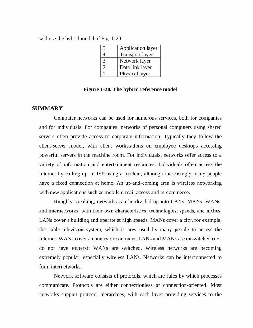
will use the hybrid model of Fig. 1-20.

5 Application layer 4 Transport layer 3 Network layer 2 Data link layer 1 Physical layer

Figure 1-20. The hybrid reference model

SUMMARY

Computer networks can be used for numerous services, both for companies

and for individuals. For companies, networks of personal computers using shared

servers often provide access to corporate information. Typically they follow the

client-server model, with client workstations on employee desktops accessing

powerful servers in the machine room. For individuals, networks offer access to a

variety of information and entertainment resources. Individuals often access the

Internet by calling up an ISP using a modem, although increasingly many people

have a fixed connection at home. An up-and-coming area is wireless networking

with new applications such as mobile e-mail access and m-commerce.

Roughly speaking, networks can be divided up into LANs, MANs, WANs,

and internetworks, with their own characteristics, technologies; speeds, and niches.

LANs cover a building and operate at high speeds. MANs cover a city, for example,

the cable television system, which is now used by many people to access the

Internet. WANs cover a country or continent. LANs and MANs are unswitched (i.e.,

do not have routers); WANs are switched. Wireless networks are becoming

extremely popular, especially wireless LANs. Networks can be interconnected to

form internetworks.

Network software consists of protocols, which are rules by which processes

communicate. Protocols are either connectionless or connection-oriented. Most

networks support protocol hierarchies, with each layer providing services to the

layers above it and insulating them from the details of the protocols used in the

lower layer. A model known as Open Systems Interconnect (OSI) was devised by

the International Standards organization (ISO). This model would allow the sending

and receiving of data between two computers.

It works on a layer approach, where each layer is responsible for performing

certain jobs and functions. The need of layered architecture arises because when

data is sent from one computer to another, there are many different things involved.

These are network adapters, voltages and signals on the cable, how the data is

packaged, error control in case something goes wrong, and many other issues. By

segmenting these issues into separate layers, it makes the task of designing network

much easier. The OSI model, which allows dissimilar computers to transfer data

between themselves, is divided into seven distinct layers.

These layers are application, presentation, session, transport, network, data

link and physical layer with their distinct functions. These functions are to provide

applications with access to network, determine the format used to exchange data

among computer over the network, allow connection disconnection to be established

between applications, allow error free delivery of data and send data at correct

destination.

TCP/IP is the protocol used by computers on the internet and may be

considered as two separate protocols such as TCP and IP.

Each computer has an IP address. A protocol is a set of rules that govern how

computers talk to each other. TCP/IP is a widely used and very popular protocol.

With TCP/IP, different computer systems can reliably exchange data on an

interconnected network. It also provides a consistent set of application programming

interfaces (APIs) to support application development. This means that software

programs can use TCP/IP to exchange data. An example of this is web servers and

web browsers, software applications that use TCP/IP to exchange data.

Protocol stacks are typically based either on the OSI model or on the TCP/IP

model. Both have network, transport, and application layers, but they differ on the

other layers. Design issues include multiplexing, flow control, error control, and

others.

Networks provide services to their users. These services can be connection

oriented or connectionless. In some networks, connectionless service is provided in

one layer and connection-oriented service is provided in the layer above it. Well-

known networks include the Internet, ATM networks, Ethernet, and the IEEE

802.11 wireless LAN. The Internet evolved from the ARPANET, to which other

networks were added to form an internetwork. The present Internet is actual ally a

collection of many thousands of networks, rather than a single network. What

characterizes it is the use of the TCP/IP protocol stack throughout. ATM is widely

used inside the telephone system for long-haul data traffic. Ethernet is the most

popular LAN and is present in most large companies and universities. Finally,

wireless LANs at surprisingly high speeds (up to 54 Mbps) are beginning to be

widely deployed.

1.11 Self Assessment Questions

1. Define the following

(a) Workstation

(b) Server

(c) Network interface Unit

2. What is network topology ? Explain the following with suitable example and

their relative advantages and disadvantages.

(a) Star topology

(b) Bus topology

(c) Ring topology

(d) Tree topology

(e) Hybrid topology

3. (a) Differentiate between LAN, MAN and WAN.

(b) Differentiate between connection oriented and connectionless services.

4. Describe the OSI reference model and explain the function of each layer.

5. Critically compare OSI reference model and TCP/IP model.

6. Explain the functions of different layers of TCP/IP reference model and

various protocols working in these layers.

Suggested Readings

1. Tannenbaum,”Computer Network”, Pearson Education

2. Godbole,”Data Communications and Networking”, Tata Mc Graw-Hill

3. Forouzan,” Communications and Networking”, Tata Mc Graw-Hill

Subject : Computer Network

Paper Code : 301 Author : Dharmender Kumar

Lesson No. : 02 Vetter : Dr. Yogesh Chaba

Chapter Title : Data Transmission

Topics

2.0 Objective 2.1 Theoretical Coverage of Basis of Data Communication

2.1.1 Introduction to Analogue and Digital Signal 2.1.2 Amplitude, Period, Frequency and phase 2.1.3 Fourier Analysis & Concept of Bandwidth of a Signal 2.1.4 Maximum Data rate of a channel

2.2. Transmission Media 2.2.1 Guided Media

Twisted Pair Cable Coaxial Cable Optical Fibre 2.2.2 Unguided Media Radio Communication Microwave Communication Satellite Communication Cellular (Mobile) Communication 2.3. Types of Transmission

2.3.1 Parallel Communication 2.3.2 Serial Communication 2.3.3 Asynchronous Communication 2.3.4 Synchronous Communication 2.3.5 Isochronous Communication 2.3.6 Simplex, Half Duplex, Full Duplex Communication

2.4 Summary 2.5 Self Assessment Questions

2.0 Objective : To Learn about the various concepts related to data communication, Transmission Media available and various types of data transmission. 2.1 Theoretical Coverage of Basis of Data Communication

At the core of all computer to computer data communications is the concept

of signal propagation. The simple idea in signal propagation is that when a signal

is applied in any form (such as heat, voltage or current) to one end of a conducting

material, after some time the signal reaches the other end of the material. Thus, a

wire can also be used for carrying data between the two points that it connects.

2.1.1 Introduction to Analog and Digital Signals

Any Signal can be classified into one of the two types : analog and digital.

An analog signal is a continuously varying signal, similar to a sinusoidal

waveform. For instance, if we measure the room temperature continuously and

plot its graph with the time on the x-axis and the temperature on the y axis, we

would get a continuous waveform, which is an analog signal. Analog is always

continuous.

In contrast, a digital signal takes the form of pulses, where we have

something or nothing, (i.e. 1 or o in digital terms). The absence or presence of

something (i.e. 0 or 1) can be used to plot a digital signal. A typical digital signal

is shown in Fig. (2.2)

Fig. 2.1 Fig. 2.2

Fig 2.3 Digital Signal

Thus, we can say that an analog signal is smooth and continuous in nature.

In contrast, a digital signal represents a sudden jump from one value to another. A

digital signal for bits 0110 10 is shown in Fig. 2.2 where 0 means no voltage and

1 means some +ve voltage.

Again, regardless of whether the signal is analog or digital, if we apply this

signal at one end of the wire, the signal form will travel at the other end (with

some distortions caused due to noise, which we shall study later). For instance let

us imagine that we have a wire A-X-B (like the one shown in (Fig. 2.3). Let us

imagine that we apply 0 voltage to point A for some time (representing 0), then 5

volts for a longer duration (representing 11), then again 0 voltage for some time

(representing 0) and so on. It will mean that we are applying a digital signal as

shown, in Fig. 2.2, at point A. Due to the principle of signal propagation, the same

signal (i.e. 011010 in this case) will traverse to point X and then to point B with

some distortion and after a finite propagation delay.

2.1.2 Amplitude, Period, Frequency and Phase

At any point, the strength of the signal or amplitude is given by the Y-axis.

Thus, the amplitude of a signal is equal to its vertical distance from the horizontal

X-axis. Fig 2.4. shows that the signal has maximum value, called amplitude (A)

shown as A at point K. Amplitude is measured in volts (representing voltage),

amperes (representing current) or watts (representing power), depending on the

type of the signal.

Fig. 2.4 Sinusoidal Signal

We see that the signal repeats itself; i.e. completes one cycle after time T.

That is, the signal reaches the peak and comes back to its original starting position

in time T. The time taken for the completion of one cycle is called period, which is

shown as 1/10th of a second in the figure. This is because the particle in our

example in Fig.2.4(a) was rotating at ten revolutions per second. This means that

the signal value will be same at times t and t + 1/10th of a second, for any value of

t. Period is expressed in seconds, or smaller units of a second, such as milliseconds

or ms (i.e. 10-3 seconds), microseconds or MS (i.e. 10-6 seconds), nanoseconds or

ns (i.e. 10-9 seconds), or pico-seconds or ps (i.e. 10-12 seconds). Another term

which is used very often is frequency. The frequency (f) is the number of cycles or

periods a signal completes in one second. We can notice that this would be same

as the number of revolutions that our particle would make in one second. Figure

2.4 shows that f = 10.

It can be easily shown that f = 1/T. For instance, in our example, T = 1/10th

of a second, i.e. the signal completes one cycle in 1/l0th of a second. Therefore, in

one second, it will complete 1/(1/10) = 10 cycles. Therefore the frequency of this

signal is 10, i.e. f = 10 cycles per second and f= l/T.

Frequency is measured in Hertz (Hz), named after a German mathematician. One

Hz is one cycle/ second Therefore, in the example above, the frequency is 10 Hz.

We use one Kilohertz or one kHz to mean 1000 Hz, and one Megahertz or one

MHz to mean 1000 kHz or 1000000 Hz..

2.1.3 Fourier analysis and the concept of bandwidth of a signal

Now we return to Fourier's theory. How can we decompose a random

signal, such as generated by a telephone conversation into various sinusoidal

signals of varying amplitudes. frequencies and phases? We do not want to give a

mathematical proof of this here. We will just take an example to illustrate this

concept.

Figure 2.5 (a), (b) and (c) show three sinusoidal signals with different

amplitudes and frequencies (e.g. 10Hz, 30Hz and 50Hz). In Fig.(a), the signal

completes one cycle in l/10th of a second, i.e. its frequency = 10 Hz (10

cycles/sec). Similarly. it is easy to see that the signals in Fig. 2.5(b) and (c) have

frequencies 30 and 50, respectively.

Fig. 2.5 Fourier Analysis Illustrated

For every value of time t on the X-axis, if we add the signal strength

(amplitude) of these three signals and plot the result as the signal strength of the

resultant signal on the Y-axis, we get the resultant analog signal as shown in Fig.

2.5(d). For instance, if we add Y I, Y2 and Y3, we will get Y 4, all at time = 10. If

we do that for all values of t, we will get the resultant signal shown in Fig. 2.5(d).

Conversely, we can show that the analog signal shown in Fig. 2.5(d) is derived out

of superimposing the three sinusoidal signals in Figs 2.5(a), (b) and (c). Similarly,

it can be shown that any signal can be decomposed into different sinusoidal

signals. This process is called Fourier analysis.

We can now understand that if we carry out a Fourier analysis on any

complex signal, we will get a set of sinusoidal signals of different frequencies.

Now, if we find out the difference between the highest and the lowest frequencies

from within the sinusoidal signals making up that complex signal, we get a very

useful concept. We call this difference bandwidth of the complex signal. For

instance, the bandwidth of the signal in Fig. 2.5(d) is 50 Hz-10Hz = 40 Hz. The

simplest way to describe bandwidth is the fastest continually oscillating signal that

can be sent across a wire.

Example

A periodic signal has been decomposed using Fourier analysis to yield four sine

waves of frequencies 100,400,600 and 800 Hz. What is the bandwidth of the

resulting periodic signal?

Solution

We know that the bandwidth of a signal is the difference between the highest and

the lowest frequencies. Therefore, the bandwidth of the periodic signal = 800-100

= 700 Hz.

Example

A signal has a bandwidth of 20 Hz and its highest frequency is 60 Hz. What is its

lowest frequency?

Solution

Since the bandwidth of a signal is the difference between its highest and lowest

frequencies, in this case, we have the following solution:

Lowest Frequency = Highest Frequency - Bandwidth = 60 - 20 = 40 Hz.

Similarly, we can find out the bandwidth of any signal of any shape and

size. It is clear that if the signal changes very rapidly (as in a video signal), the

higher frequency will be very high, i.e. when we decompose this signal into

various sinusoidal signals, there will be some with very high frequencies.

Therefore, the bandwidth of such signals will be very high. If the signal

changes very slowly, its bandwidth will be very small. At an extreme, a digital

signal has both horizontal and vertical lines, and therefore, signals with 0 and 00

frequencies. Therefore, the bandwidth of a digital signal is 00 - 0 = 00. We will

return to this theme shortly.

We must point out that similar to the bandwidth of a signal, there is a

bandwidth of a medium. What does this mean? Suppose that we have a thin water

pipe and a very forceful water flow. The thinness of the water pipe (i.e. the

medium) in such a case represents the fact that its bandwidth is quite small as

compared to the bandwidth of the water (i.e. the signal) that needs to be carried

through it. Thus, both. a signal and the medium that is to carry the signal have

their own bandwidths.

As we can imagine, even in the case of a medium, its bandwidth is the

difference between the maximum and the minimum frequencies that it can carry.

For many media (except the radio), the minimum frequency is 0. Therefore,

generally, the bandwidth of a medium is also the same as the maximum frequency

that it can carry. Why should there be a limit on this highest frequency? The

reason lies in the nature of the medium. Depending on the metal or the material

used for the medium (i.e. the free electrons, etc), changes in the signals at one end

are transmitted to the other end faithfully only up to a particular rate at which the

signal changes (i.e. frequency). If this rate increases more than a certain limit,

before the change in the signal is transmitted from points A to B, the signal at

point A would change, and therefore, faithful transmission would not be possible.

The signal would get distorted beyond repair. In simple terms, if the sender

attempts to transmit signals that are faster than the bandwidth, the underlying

hardware would not be able to keep up with the pace, because it would not have

sufficient time to complete one change before the sender attempts to send another.

This defines the maximum rate at which hardware can change a signal, i.e. the

bandwidth of a medium. As we shall see, the bandwidth of optical fiber is far more

than that of coaxial cable, which, in turn, is far higher than that of a twisted wire

pair.

2.1.4 The Maximum Data Rate of a Channel

As early as 1924, an AT&T engineer, Henry Nyquist, realized that even a

perfect channel has a finite transmission capacity. He derived an equation

expressing the maximum data rate for a finite bandwidth noiseless channel. In

1948, Claude Shannon carried Nyquist's work further and extended "it to the case

of a channel subject to random (that is, thermodynamic) noise (Shannon, 1948).

We will just briefly summarize their now classical results here.

Nyquist proved that if an arbitrary signal. has been run through a low-pass

filter of bandwidth H, the filtered signal can be completely reconstructed by mak-

ing only 2H (exact) samples per second. Sampling the line faster than 2H times

per second is pointless because the higher frequency components that such sam-

pling could recover have already been filtered out. If the signal consists of V dis-

crete levels, Nyquist's theorem states: .

maximum data rate = 2H log2 V bits/ sec

For example, a noiseless 3-kHz channel cannot transmit binary (i.e., ,two-level)

signals at a rate exceeding 6000 bps.

So far we have considered only noiseless channels. If random noise is pres-

ent, the situation deteriorates rapidly. And there is always random (thermal) noise

present due to the motion of the molecules in the system. The amount of thermal

noise present is measured by the ratio of the signal power to. the noise power,

called the signal-to-noise ratio. If we denote' the signal power by S and the noise

power by N, the signal-to-noise ratio is S/N. Usually, the ratio itself is not quoted;

instead, the quantity 10 log 10 S/N is given. These units are called decibels (dB).

An S/N ratio of 10 is 10 dB, a ratio of 100 is 20 dB, a ratio of 1000 is 30 dB, and

so on. The manufacturers of stereo amplifiers often characterize the bandwidth

(frequency range) over which their product is linear by giving the 3-dB frequency

on each end. These are the points at which the amplification factor has been ap-

proximately halved (because log l03 ≈0.5).

Shannon's major result is that the maximum data rate of a noisy channel

whose bandwidth is H Hz, and whose signal-to-noise ratio is SIN, is given by

maximum number of bits/ sec = H log2 (I + S/N)

For example, a channel of 3000-Hz bandwidth with a signal to thermal

noise ratio of 30 dB (typical parameters of the analog part of the telephone system)

can never transmit much more than 30,000 bps, no matter how many or how few

signal levels are used and no matter how often or how infrequently samples are

taken. Shannon's result was derived from information-.theory arguments and

applies to any channel subject to thermal noise. Counterexamples should be

treated in the same category as perpetual motion machines. It should be noted that

this is only an upper bound and real systems rarely achieve it.

2.2 Transmission media

Transmission media are the physical infrastructure components that carry

data from one computer to another. They are at the basis of data communications.

Examples of simple forms of transmission media are telephone wires that connect

telephones to the central offices (i.e. telephone exchanges), and coaxial cables that

carry the cable television transmission to homes. Transmission media need not

always be in the form of a physical wire-they can be invisible as well We shall

study these different types of transmission media in this chapter.

Broadly, all transmission media can be divided into two main categories:

Guided and Unguided, as shown in Fig. 2.6.

2.2.1 GUIDED MEDIA

Guided Media can be further subdivided into three main types as shown in

Fig.2.8 Guided media are typically based on some physical cable. Twisted pair

and coaxial cables carry signals in the form of electrical current, whereas optical

fiber carries signals in the form of light. We will now study these one by one.

1. Twisted Pair Cable

There are two classes of twisted pair cables as shown in fig. 2.8

a. Unshielded Twisted Pair (UTP)

This is the most commonly used medium today, because of its usage in the

Transmission Media

Guided Media Unguided Media

Fig2.6 Categories of Transmission Media

Guided Media

Twisted Pair Wires Coaxial Cables Optical Fiber

Fig 2.7 Types of Guided Media

Twisted pair Cable

Unshielded Twisted Pair

Shielded Twisted Pair (STP)

Fig 2.8 Categories of Twisted Pair Cable

telephone system. This cable can carry both voice as well as data. It consists of

two conductors (usually copper). In the beginning, the wires used to be kept

parallel. However, this results in far greater levels of noise. Hence, the wires are

normally twisted as shown Fig. 2.9. This results in the reduction of noise to a great

extent, although it is not eliminated completely. The copper conductors are

covered by Fig. 2.9 PVC. or other insulator.

Fig. 2.9 Unshielded Twisted Pair (UTP)

UTP is flexible, cheap and easy to install. The Electronic Industries Association

(EIA) has developed standards for UTP cables. They are given in Fig. 2.10. Each

one is manufactured differently for a specific purpose.

Category Usage

1. The basic cable used in the telephone system. This is fine for

voice communication, but is unsuitable for data

communication, except at very low speed.

2. Suitable for voice and data communication up to the speed of

4 Mbps.

3. Can carry voice and data up to 10 Mbps. It requires minimum

three twists per foot. Today, these are more regularly used in

telephone networks.

4. These are similar to the category 3, but can handle data up to

16 Mbps.

5. Can handle data speed of 100 Mbps.

Fig.2.10 Categories of UTP

Today, UTPs of higher categories are also used in computer

networks given the higher speeds and reliability.

b. Shielded Twisted Pair (STP)

In this case, apart from the insulator, the twisted wire pair itself is covered

by metal shield and finally by the plastic cover as shown in Fig. 2.11. The metal

shield prevents penetration of electromagnetic noise. It also helps eliminate

crosstalk, an effect wherein one wire picks up some of the signals travelling on the

other wire. This effect can be felt sometimes during telephone conversations,

when we hear other conversations in the background during our call. The shield

prevents such unwanted sounds.

As we have seen, the shield reduces the noise and cross talk (noticed in the

telephone calls sometimes1'Substantially. However, STP is more expensive than

UTP.

2 Coaxial Cable

Coaxial cable (also called as coax) has an inner central conductor

surrounded by an insulating sheath, which in turn is enclosed in the outer

conductor (shield). This acts not only as a second conductor for completing the

circuit but also acts as a shield against noise. This outer conductor is covered by a

plastic cover. This whole arrangement is shown in Fig. 2.12

Fig 2.11. Shielded Twisted Pair (STP)

Fig. 2.12 Coaxial Cable

Compared to UTP or STP, coaxial cable is more expensive, less flexible

and more difficult to install in a building where a number of twists and turns are

required. However, it is much more reliable and can carry far higher data rates.

Coaxial cables are divided into various categories depending upon the thickness

and size of the shields, insulators and the outer coating and other considerations.

They are commonly used by cable companies to carry cable transmissions.

The various coaxial cable standards are RG-8, RG-9, RG-11, RG-58 and

RG-59.

3 Optical Fiber

Optical Fiber Structure

Optical fibers use light instead of electrical signals as a means of signal

propagation. They are made of glass fibers that are enclosed in a plastic jacket.

This allows the fibers to bend and not break. A transmitter at the sender's end of

the optical fiber sends a light emitting diode (LED) or laser to send pulses of light

across the fiber. A receiver at the other end makes use of a light-sensitive

transistor to detect the absence or presence of light to indicate a 0 or a 1.

In the fiber, the cladding covers the core (fiber) depending upon the size.

Commonly, the fiber is covered by a buffer layer, which protects it from moisture.

Finally, an outer jacket surrounds the entire cable. This is shown in Fig. 2.13

Fig 2.13. Optical Fiber

The core and cladding must be extremely pure, and should not vary in size

or shape. The outer jacket, however, can be made of Teflon, plastic or metal.

Teflon is more expensive than plastic, but both do not provide the structural

strength to the fiber. Metal can provide that, but is very heavy and expensive. The

choice depends upon many of these factors.

Light Source for Fiber

For data transmission. to occur, the sending device must be capable of

inducing data bits 0 to I into the light source and the receiving device must have a

photosensitive cell called photodiode, which would translate this light back again

into data bits.

There are two types of light sources: Light Emitting Diode (LED) and

Injection Laser Diode (ILD). LED is cheaper but it provides unfocussed light that

hits the boundaries of the core at different angles and diffuses over distance. This

is why LED is used only for a short distance. Laser, however, can provide a very

focused beam, which retains its character over a long distance.

Light travels at a speed of 300,000 km/second or 186,000 miles/second in a

straight direction as long as it moves through a uniform substance. However, when

the medium through which the light passes changes, its speed and therefore, the

direction, also changes suddenly. A spoon half immersed in the glass of water

appears bent due to the same reason. This phenomenon is called as refraction.

If we change the direction of the incoming light, the direction of the

refracted light also changes as shown in Figs. 2.14(a), (b) and (c). Finally, we

reach a stage where the refracted light becomes horizontal as shown in Fig.

2.14(d). After this stage, if the angle still changes, the light is not refracted,

instead, it is reflected, as shown in Fig. 2.14(e).

Fig 2.14 Reflection and Refraction

Optical fibers use reflection to guide the light through the optical fiber. A

glass or plastic core is surrounded by a cover of less dense glass or plastic. The

difference in the densities of the two is adjusted such that reflection, instead of

refraction, occurs.

Propagation Modes

There are different modes of propagation, depending upon the physical

characteristics of the fiber and the light source. These are shown in Fig. 2.15.

Fig 2.15. Propagation Modes

Multimode

In this case, LED is mostly used as a light source. Therefore, multiple

beams pass through the core in different paths. The structure of the core decides

the way they travel.

Step Index

In this case. the core has one density and the cladding has another.

Therefore, at the interface, there is a sudden change. That is why it is called step

index. Multiple beams take different paths on

Fig 2.16 Multimode Step Index Fiber

reflection as shown in the figure 2.16. The beam that strikes the core at a smaller

angle has to be reflected many more times than the beam that shifted the core at a

larger angle to reach the other end. This means that at the destination, all beams do

not reach simultaneously, creating diffusion and in fact confusion in terms of

interpretation. This scheme is therefore used only for short distances.

Graded Index

In this case, the core itself is made of a material of varying densities. The

density is the highest at the core and gradually decreases towards the edge.

Therefore, a beam goes through gradual refraction giving rise to a curve as shown

in Fig. except that the horizontal beam travels unchanged.

Fig. Multiple graded index Fibre

In this case also, different beams result in different curves or waveforms.

Therefore, if we place the receiver at one of these intersection points, the accuracy

of the signal reconstruction is enhanced substantially.

Single Mode

This uses a highly focused light beam and travels more or less horizontally.

The fiber core diameter in this case is much smaller than multimode and also has

far lower density. This decrease results in a critical angle close to 90 degrees to

make the propagation of different beams very close to horizontal. As the

propagation of different beams is more or less similar, the delays are negligible

and the reconstruction of the signal that much easier as shown in figure 2.17.

Fig 2.17. Single Mode Fiber

Advantages of Optical Fiber

Optical fiber provides the following advantages over twisted-pair and

coaxial cable:

Resistance to noise Optical fiber uses light rays for communication, rather

than electricity. Therefore, noise is not an issue here. The only possible

source of interference is external light, which is also blocked by the outer

jacket of the optical fiber, thus providing resistance to interference.

Huge bandwidth The bandwidth offered by optical fiber is huge as

compared to twisted-pair and coaxial cable.

Higher signal carrying capacity Unlike twisted-pair and coaxial cable, the

signals carried by optical fiber travel longer distances (several kilometers)

without needing regeneration.

Disadvantages of Optical Fiber

Along with all the advantages that it offers, optical fiber also has some

disadvantages, as summarized

Fragility Optical fiber is more delicate than twisted-pair and coaxial cable,

so the chances of it breaking are higher.

Cost Optical fiber is quite expensive because it has to be extremely pure to

be able to carry signals without damage over longer distances. The laser

light source itself is also very costly, as compared to the electrical signal

generators.

Maintenance overhead Optical fibers need more maintenance overheads as

compared to twisted-pair and coaxial cable.

2.2.2 UNGUIDED MEDIA (Wireless Communication)

Unguided media, also called as wireless communication, transport

electromagnetic waves without using a physical conductor. The signals propagate

through air (or sometimes water). The communication band for unguided media is

as shown in Fig. 2.18. We shall concentrate on the radio communications.

(a) Radio Communication

Fig 2.18. Radio Communications Band

Very Low Frequency (VLF) waves propagate as surface waves, usually

through air, but sometimes also through water. VLF waves do not suffer

attenuation, but atmospheric noise affects them. VLF waves are usually

used for long-range radio navigation and submarine communication.

Low Frequency (LF) waves also propagate as surface waves. Attenuation

is higher during the daytime. These wave are used for long range radio

navigation or navigation locators.

Middle Frequency (MF) waves rely on line-of-sight antennas to increase

and control absorption problems. These waves are used for AM radio, radio

direction finding and emergency frequencies.

High Frequency (HF) waves are used for amateur radio, citizen's band

radio, international broadcasting, military communication, telephone,

telegraph and facsimile communication.

Very High Frequency (VHF) waves use line-of-sight propagation, and are

used for VHF television, FM radio, aircraft AM radio and aircraft

navigation.

Ultra High Frequency (UHF) waves use line-of-sight propagation. They

are used for television, mobile phone, cellular radio, paging and microwave

links.

Super High Frequency (SHF) waves are transmitted as either line-of-sight

or into the space. They are used for terrestrial and satellite microwave and

radar communication.

Extreme high Frequency (EHF) waves are transmitted into space, and are

used for scientific applications such as radar, satellite and experimental

communication.

(b) Microwave Communication

As shown in Fig.2.19, microwaves use the line of sight method of

propagation. as the signals do not travel along the surface of the earth. Therefore,

the two antennas must be in a straight line, able to look at each other without any

obstacle in between. The taller the antennas, the more is the distance that these

waves travel. Usually, the antennas are positioned on mountain tops to avoid

obstacles. Microwave signals travel only in one direction at a time. This means

that for two-wave communication such as in telephony, two frequencies need to be

allocated. At both ends, a transceiver is' used which is a combination of a

transmitter and a receiver operating at the two respective frequencies. Therefore,

only one antenna can serve both the functions and cover both the frequencies..

Repeaters are used along with. The antennas to enhance the signa1. The data rates

offered are 1 Mbps -10 Gbps.

Fig.2.19 Terrestrial Microwave Communication

For many decades, before fiber optics was used, microwave communication

formed an important part of telephony. The company Sprint was based on optical

fiber communication, whereas the company MCI was completely based on the

microwave communication initially. The name MCI, in fact, stood for Microwave

Communications Inc. Lately, MCI is also changing over to optical fiber. However,

microwave communication will continue to be useful as it allows you to

communicate from anywhere. Microwave is also relatively inexpensive.

(c) Satellite Communication

Satellite communications is similar to the terrestrial microwave, except that the

satellite acts as one of the stations. Figure 2.20 illustrates this. The satellite does

the functions of an antenna and the repeater together. For instance, as Fig. 2.20

illustrates, ground station A can send the information to ground station B via the

satellite.

This, however, poses a problem. If the earth along with its ground stations

is revolving and the satellite is stationery, the sending and receiving earth stations

and the satellite can be out of sync over time. Therefore, normally

Geosynchronous satellites are used, which move at the same Revolutions Per

Minute (RPM) as that of the earth in the same direction, exactly like the earth.

Thus, both the earth and the satellite complete one revolution

Fig.2.20 Satellite Microwave Communication

exactly in the same time: the relative position of the ground station with respect to

the- satellite never changes. Therefore, the movement of the earth does not matter

for the communicating nodes based on the earth. Using satellites, we can

communicate from any part of the world to any other. However, a minimum of

three satellite needed to cover the earth's surface entirely as shown in the Fig. 2.21.

Normally, SHF, which covers the frequency range of 3 GHz to 30 GHz

used for satellite communications. Two frequency bands are used for the signals

from the earth to the satellite (called uplink), and from the satellite to the earth

(called downlink).

Fig.2.21 Three Satellites to Cover the Planet

Access Methods

There are three methods for communication using satellites. These three

methods use principles that are similar in concept to normal wired communication.

Like the wired world, satellite communication is also based on modulation

techniques. The three primary modulation techniques are: (a) Frequency Division

Multiple Access (FDMA), (b) Time Division Multiple Access (TDMA) and (c)

Code Division Multiple Access (CDMA).

These technologies can be explained at a broad level by breaking down the

title of each one.

(a) The first word tells us what the access method is and the second word,

division, lets you know that it splits transmissions based on that access method.

• FDMA puts each transmission on a separate frequency

• TDMA assigns each transmission a certain portion of time on a designated

frequency

• CDMA gives a unique code to each transmission and spreads it over the

available set of frequencies .

(b) The last words of each category are multiple access. This simply means that

more than one user (multiple) can use (access) each cell. We shall now discuss

these technologies in brief.

Frequency Division Multiple Access (FDMA)

FDMA splits the total bandwidth into multiple channels. Each ground

station on the earth is allocated a particular frequency group (or a range of

frequencies). Within each group, the ground station can allocate different

frequencies to individual channels, which are used by different stations connected

to that ground station. Before the transmission begins, the transmitting ground

station looks for an empty channel within the frequency range that is allocated to it

and once it finds an empty channel, it allocates it to the particular transmitting

station.

This is the most popular method for communication using satellites. The

transmission station on earth combines multiple signals to be sent into a single

carrier signal of a unique frequency by multiplexing them, similar to the way a TV

transmission works. The satellite receives this single multiplexed signal. The

satellite, in turn, broadcasts the received signal to the receiving earth station. The

receiving station is also supposed to agree to this carrier frequency, so that it can

demultiplex the received signals. The basic idea of FDMA is shown in Fig. 2.22

Fig.2.22 Frequency Division Multiple Access (FDMA)

Time Division Multiplexing (TDMA)

Unlike FDMA, TDMA allows access to the full bandwidth of the frequency

spectrum. In TDMA, each transmitter is allocated a predefined time slot. Each

transmitter receives the time slot in turn and it is allowed to transmit data for the

duration of the time slot. This is shown in Fig. 2.23.

Fig.2.23 Time Division Multiple Access (TDMA)

After FDMA, TDMA is the second most popular mechanism for communication

using satellites. In case of TDMA, there is no modulation of frequencies (unlike

FDMA). Instead, the transmitting earth station transmits data in the form of

packets of data. These data packets arrive at the satellite one by one (hence the

name TDMA). By the same logic that was discussed during TDM, TDMA is also

a digital form of data transmission; TDMA operates in time domain, rather than

frequency domain. Bit rates of 10-100 Mbps are common for TDMA

transmissions. This can be translated into roughly 1800 simultaneous voice calls

using 64 Kbps PCM.

Code Division Multiple Access (CDMA)

As we have seen, in FDMA, a fixed frequency channel is allocated to a

transmission pair (i.e. the transmitter and the receiver). In the case of TDMA,

transmission happens by using predefined time slots. Nothing of this sort happens

in the case of CDMA. CDMA allows any transmitter to transmit in any frequency,

and at any time. Thus, it is different from both FDMA and TDMA.

An obvious question is: Would this not lead to confusion and mixing of

different signals? It would. However, to counter this, the transmitter and the

receiver agree upon a unique coding scheme (similar to encryption) before the

start of the transmission. The analogy often used to explain CDMA is an

international party, where there are dozens of people. All are talking at once, and

all talking in different languages that you do not understand. Suddenly, from

across the room, you hear a voice speaking in your own familiar language, and

your brain tunes out all the background gibberish and locks onto to that one

person. Your brain understands the code being used by the other person, and vice

versa.

Similarly, CDMA uses coding that is unique to a particular transmission

and allows the receiver to disregard other transmissions on the same frequency. In

this case, the coding scheme is a unique frequency with which the original signal

is modulated to form the codified signal that is to be transmitted. The transmitter

then codifies all its transmissions in this manner, before they are sent. Since only

the receiver knows how to decode this (as agreed upon before the start of the

transmission), there is no scope for confusion. This is shown in Fig.2.24.

Fig.2.24 Code Division Multiple Access (CDMA)

CDMA is the newest and the least used access method using satellites. It is

popular in military installations, but not so much in the case of commercial

applications.

d. Cellular (Mobile) Communication

The city of St. Louis in the USA saw the emergence of the first

mobile telephone as early as 1946. This system was difficult to operate and had a

single channel for both sending and receiving. You had to push a button to enable

the transmitter and disable the receiver. This half-duplex system, known as push-

to-talk-system, was installed in the big cities in 1950s. Even today, taxis, CB-radio

etc. use the same technology.

The second development took place in 1960s. This was called Improved

Mobile Telephone System (IMTS). It had a strong transmitter, and used two

frequencies. One frequency was used for sending and the other for receiving. This

full-duplex system had 23 channels and was a great improvement over the push-

to-talk-system. However, in IMTS too, users had to wait for a long time to get a

dial tone.

The third step was the development of Advanced Mobile Phone System

(AMPS). In England, it is called TACS and in Japan, MCS-Ll. In this scheme, the

area covered is conceptually divided in small regions known as cells, thus the

name cellular phones. Though the cells are actually circular, they are shown as

hexagonal for conceptual clarity in the figure that follows. Each cell has an

antenna and a cell office to control that cell. A Mobile Telephone Switching

Office (MTSO) controls various such cell offices and coordinates the

communication between them and the Telephone Central Office (TCO) or a

telephone exchange. The TCO is a part of the wired land telephone system. The

computer at MTSO is responsible for not only the connections but also for the

information and billing of the calls. The typical cell radius size is 0 to 12 miles.

However, it can be changed, depending upon the population in the area. The whole

cellular phone systme is described in the fig. 2.25 shown below.

Fig.2.25 Cellular Phone System

Bands in Cellular Telephony

Classically, analog transmission is used for cellular telephony. Frequency

modulation is used for communication between the mobile phone and the cell

office. Normally, two frequency bands are allocated for this purpose. One of them

is for the communication that is initiated by the mobile phone and the other for the

land phone. However, each channel requires a full-duplex dialog. For preventing

interference, adjacent channels are rarely allocated. Some channels are also

required for control purposes. This reduces the number of channels available for

each cell. This number is 40 in USA today. However, the same frequency band

can be used for multiple non-adjacent cells as shown in Fig. 2.26. In USA, FCC

controls these bands. The two bands are typically 824-849 MHz and 869-894

MHz.

Fig. 2.26 Frequency Reuse

Calls Using Mobile Phones

When a call is made from the mobile phone by entering a 7-,8- or lO-digit

phone number, the mobile phone itself scans the band and seeks a channel for

setting up the call. After this, it sends this number to the closest cell office, which,

in turn, sends it to MTSO. The MTSO, in turn, sends it to the CTO. If the called

party is available, CTO lets MTSO know. At this juncture, MTSO allocates an

empty voice channel to the cell to establish the connection. The mobile phone

adjusts its tuning to the new channel and the dialog begins.

When a land phone places a call to a mobile phone, the telephone central

office sends the number to the MTSO. The MTSO performs a lookup to see where

the mobile phone is currently placed by sending appropriate query signals to all

the cells. This process is called paging. The cell where the mobile phone is

currently located responds to the MTSO. The MTSO then transmits the incoming

call signal to that mobile phone, and when the mobile phone is answered, the

MTSO assigns a voice channel to the call, thus enabling the conversation.

Transmitting/Receiving/Handoff Operations

During the conversation, if the mobile phone crosses the cell, the signal can

become weak. The MTSO constantly checks the signal level, and if it finds it low,

it immediately seeks a new cell that can look after the communication better. The

MTSO then changes the cell-carrying channel so smoothly that the user hardly

notices. This process of handling the signal off from the old channel to the new

one is called handoff. This process is described below.

Step 1: Cell A senses that the user of cell 50 is moving to cell B, and that its signal

is becoming weaker. So, it alerts the MTSO. This is shown in Fig. 2.27

Fig.2.27 Handoff Part l-A Unit Becomes Weak in Cell A

Step 2: The MTSO wants to check if any of the adjacent units (B, C, etc.) can take

up the responsibility of unit 50. Cell C responds by saying that it cannot do so, as

unit 50 is weak in cell C, too. However, cell B says that it is ready to take up the

responsibility of unit 50 as it is receiving a strong signal from unit 50. This is

shown in Fig. 2.28.

Step 3: The MTSO redirects unit 50 from cell A to cell B. This is shown in Fig.

2.29

Fig. 2.28 Handoff Part 2 – MTSO Enquires to see if Anybody can take up unit 50

Fig. 2.29 Handoff Part 3 – MTSO Hands over Unit 50 to Cell B

New Developments

Three developments will take place in the near future. One is digital cellular

telephone. The second is the integration of cellular phones with satellite

communication. This will enable a person to have a unique but same telephone

number throughout the world, unlike today, when we have different numbers for

land phones and mobile phones. The third is the integration of the mobile

telephony with the PC. The scheme is called Mobile Personnel Communication,

which will allow people to use a small, mobile PC to send and receive multimedia

information in all forms: data, voice, image and video.

Figure 2.30 summarizes the various transmission media in terms of their

characteristics and other features.

Medium Speed Cost Security Attenuation

UTP 1-100 Mbps Low Low High

STP 1-150 Mbps Medium Low High

COAX 1 Mbps-1 Gbps Medium Low High

Fiber 10 Mbps-2 Gbps High High Low

Radio 1-10 Mbps Medium Low High-Low

Terrestrial

Microwave

1 Mbps-10 Gbps High Medium Variable

Satellite

Microwave

1 Mbps-10 Gbps High Medium Variable

Cellular 1.6-1.2 Kbps High Low Low

Fig.2.30 Transmission Media Characteristics

Shannon Capacity

Regardless of whether it is a guided or unguided medium, every

transmission medium has a finite data carrying capacity. We are normally very

interested in knowing how much data a particular transmission medium can carry.

Claude Shannon solved this mystery in 1944 by introducing a formula that

determines the maximum data rate of a channel. This is called as the Shannon

capacity.

Shannon capacity essentially depends on one basic factor of a transmission

medium: its signal-to noise ratio. Understanding how to calculate signal-to-noise

ratio would take us to physics, therefore, we shall avoid it. Instead, we shall have a

look at the formula to determine the maximum data rate of a transmission medium

(called as Shannon capacity). The formula reads:

C = B log2 (1 + S/N)

C is the Shannon capacity in bps, B is the bandwidth of the transmission

medium, and SIN is the signal-to-noise ration of the transmission medium.

For instance, let us calculate the theoretical upper limit of transmission rate

through a normal telephone channel. Normally, a telephone channel has a

bandwidth of 3000 Hz (300 to 3300 Hz). The SIN ration is usually around 3162.

Thus, its capacity C will be:

C = B log2 (1 + SIN)

= 3000 log2 (1 + 3162)

= 3000 log2 (3163)

= 3000 x 11.62

= 34,860 bps or 34.860 Kbps

This signifies that no matter how hard you try, you cannot transmit more

than 34.860 Kbps data through a telephone line. To achieve higher transmission

rates, you must try and improve the S/N ratio.

Thus, Shannon capacity formula informs engineers that no amount of

intelligent encoding can break the laws of physics that place a basic limit on the

number of bits that can be transmitted per second over a communications system.

2.3 Types of Transmissions

Digital data can be transmitted in a number of ways from the source to the

destination. These modes of data transmission can be outlined as follows:

• Parallel and serial communication

• Asynchronous, synchronous and isochronous communication

• Simplex, half-duplex and full-duplex communication

These techniques will be discussed first followed by the concept of multiplexing.

Multiplexing allows more than one signal to be sent on a single transmission path

using techniques that help a more effective use of the transmission medium than is

possible otherwise.

2.3.1 PARALLEL COMMUNICATION

Imagine that we want to send digital data stored as bytes of 8 bits each, and

in words of may be 16 or 32 bits, depending upon the word length;

In parallel communication, we transfer a word or a byte at a time.

Therefore, we need to have those many wires parallel to each other, each carrying

a single bit. This is shown in Fig.2.31, where eight wires are transmitting a byte at

a time. In this example, the byte contains 10011001.

This is a very fast method of transmitting data from one place to another.

However, there are problems in this scheme. In the first place, it a very expensive

method because it requires several wires in sending as well as receiving

equipment. In addition, it demands extraordinary accuracy, which cannot be

guaranteed over long distances. The digital pulses ma not traverse at the same

seed, because the underlying media through which the data passes from one

computer system to another may not be exactly identical. This gives rise to a

problem of skew. as shown in the Fig. 2.32.

Fig. 2.31 Parallel Transmission Fig.2.32 The Problem of Skew

When a message is skewed, the bits 10011001 are sent from the source to

the destination, but they traverse at different speeds At the...destination, the

measurement of signal values to determine whether it was a bit 0 or 1 have to be

done at the same time for all the bits. Therefore, the problem of skew can result In

an inaccurate interpretation of bits.

To avoid this problem, parallel transmission is used only for a very short

distance and there too, all the parallel wires have to De absolutely identical. This

method is used for data transmission within the computer system, such as from the

CPU registers to the memory or vice versa through the data bus. The data bus

essentially implements the parallel transmission of data. This is done because

speed, rather than cost, is of paramount importance in this case. However, in view

of the problems outlined above, this method cannot be used over long distances.

2.3.3 Serial Communication

Over long distances, serial communication is used. While sending the data

serially, characters or bytes have to be separated and sent bit by bit. Thus, some

hardware is needed to convert the data from parallel to serial. At the destination,

the measurement of the signal values is done in the middle of the bit duration as

shown in Fig. This is because, if the values are taken at the edge or a point where

the pit value changes (shown as point A in the figure), the reading will be

indeterminate.

At the destination, all the bits are collected, measured and put together as

bytes in the memory of the destination. This requires conversion from serial to

parallel.

Fig 2.33. Serial Transmission

In serial data transmission, we have to identify where the character starts.

We have to identify where the character starts. We have to also identify the middle

position of each bit interval so that measurement can be taken. Normally, the

transmitter and the receiver have two different clocks. The point is to synchronize

the clock of the receiver exactly with that of the transmitter, so that correct

readings will result and the bit values are understood correctly. This is essentially

a problem of synchronization. We can take an example to illustrate this.

Let us say that we have to send 8 bits b0 to b7 from point X to point Y as shown in

Fig. 2.34 We have arranged the bits in a circular fashion to illustrate the point

better. Let us say that arms Al and A2 at point X and Y rotate in clockwise

directions. When both Al and A2 point to the bit 1'0 at X and Y respectively, the

connection is made and the bit b0 is transferred from X to Y. Now due to rotation,

after some time, Al will point towards bl at point X. At that time A2 also has to

point to bl. at point Y. Otherwise the bit will not be transferred correctly. The same

is true for the transfer of b2 through b7 as A I and A2 rotate clockwise. Therefore,

the two arms A I and A2 have to be perfectly synchronized and they have to rotate

at the same speed in order to succeed in sending/receiving all the bits accurately.

Fig 2.34. Serial Transmission and Synchronization

In order to achieve this, initially, we have to adjust and synchronize the

clocks in the electronics of 'the source and the destination. There are three ways in

which this can be achieved. These are: asynchronous, synchronous and

isochronous transmission. We will look at them very shortly.

A line adapter or interface generally achieves this task of synchronization. It

achieves a few other things also. We will call it only serial interface in this text.

Electronics devices called Universal Asynchronous Receiver Transmitter

(UART) and Universal Synchronous Asynchronous Receiver Transmitter

(USART) are examples of such an interface. USART can be used for both the

asynchranous and synchronous transmission. On the other hand, UART is used

only when the transmission is asynchronous.

2.3.3 ASYNCHRONOUS COMMUNICATION

Asynchronous Communication

We have learnt why serial communication is preferred to parallel

communication over a long distance. However, we have only one problem in serial

communication. How do we identify individual bits? Essentially, the problem is

that of synchronizing the sender (source) and the receiver (destination) as outlined

above.

In asynchronous communication, the time when a character will be sent

cannot be predicted. Imagine, for instance, data entry operator. She may key in a

few characters, then may consult her colleague, then key in a few more characters

before she goes off for lunch. In such a scenario, where the data is transmitted as

characters and at an unpredictable pace, we have to synchronize the source and

destination for each character. This is called asynchronous communication.

In this case, each character is preceded with a start bit and succeeded with

1, 1.5 or 2 stop bits. Figure 2.35 depicts this. Normally NRZ-L signaling is used

for asynchronous transmission. According to this convention, a negative voltage

denotes a binary 1 bit and a positive voltage denotes a binary 0 bit. When the line

is idle i.e. when no character is being sent over the line, a constant negative

voltage signifying a binary 'l' is generated.

When the character is to be sent, bit 0 is sent first. This positive voltage is

called the start bit. All the bits of the character, according to the coding

scheme used (ASCII/EBCDIC), then follow, each of which could have a 0

or 1 value.

A parity bit, if used, then follows

In the end, 1, 1.5 or 2 stop bits are added. The stop bit again corresponds to

the idle state, which is bit 1. In this context 1.5 bits only means that the

signal with negative voltage denoting 1 is generated for 1.5 times the

normal bit interval.

The sender and receiver have to exactly agree on the number of bits that represent

a character (7 or 8), the parity bit scheme if used, the bit interval (or bit rate) and

also what represents 0 and 1 (e.g. NRZ-L).

Fig. 2.35 Asynchronous Communication

Essentially, when the start bit is recognized by the destination, it knows that

a character is being sent. It then adjusts and starts its clock so that measurement of

signal values can now start at the middle of every bit that follows for the expected

number of bits. After all the bits in the character including the parity bit are

measured and stored, it expected a stop bit, which is encountered if everything is

OK. This is to recognize the bits being sent. This continues until the stop bit is

received. At this time, the, line becomes idle, and the destination clock also goes

to sleep. On receiving the start bit, it wakes up for the duration of that character,

and after the full character is received, again goes to sleep until the next character

arrives. This makes sense where (a) the rate at which the characters arrive is

unpredictable and (b) the speed at which the characters are keyed in is far less than

the speed with which they are transmitted or processed.

There has to be a proper understanding between the source and destination about

the bit rate, in bps, from which the bit interval can computed to determine when

the signal measurements have to be taken. Using this. the destination waits for the

start bit and then starts its clock to measure values to recognize the bits including

the parity bits.

2.3.4 Synchronous Communication

In synchronous transmission, the whole block of data bits is transferred at

once, instead of one character at a time. The block of bits mayor may not consist

of different characters. It could well be a digitized image. It could be anything. In

the latter case, we need a bit-oriented protocol between the sender and the

receiver. If the block of bits consists of different characters, the receiver needs to

know the beginning of the first bit of the first character. It can then start its clock

and start sampling to determine the bit values. Knowing the number of bits per

character, it can now recognize the character and store them at the destination.

This is shown in Fig. 2.36. In this case, we need to have a byte-oriented protocol

between the sender and the receiver.

Fig. 2.36 Synchronous Communication

The point is: How does the receiver know the first bit of the first character,

or when to start the clock for sampling? In order to perform this synchronization,

each data block is preceded with a unique synchronizing bit pattern. We use the

SYN (abbreviation of synchronize) transmission control character for this. It has a

bit pattern of 0010110. This bit pattern is generally not used in any normal

communication. Therefore, this SYN character can be reserved for indicating the

start of the block, i.e. for synchronization.

However, there is a problem in this scheme. The transmitter will not send a

SYN character as a part of the data. However mistake, the bit pattern of two

characters could he such that if sent one after the other. They can constitute a SYN

character, thereby fooling the receiver. Figure 2.37 illustrates this case. In this

case, if the ASCII characters b and a are sent one after the other, we get a bit

combination of 4 bits from the ASCII character band 3 bits from the ASCII

character a to constitute the SYN character.

Fig. 2.37 A Misleading SYN Character

At the receiving end, if the receiver is all the time looking for SYN characters, it

can get fooled. It is for this reason that normally two SYN bytes are sent

consecutively. The bit combination of two SYN bytes-Leo 00101100010110--

cannot be obtained by concatenating any characters. Therefore, the receiver is

asked to look for two SYN characters. If not found, it is asked to throw them off.

In some systems even three or four SYN characters are sent to make sure that

proper synchronization takes place. The receiver gets ready after receiving the

required SYN character(s) and then starts its clock for measuring the bit values for

the actual data. This is shown in Fig. 2.38.

Fig. 2.38 Discarding Non-SYN Characters Until SYN is Received for Synchronization

When the clock starts measuring the bit values, the counter within a receiver is

increment every bit receive and Measured and pushed into the character

assembler within the receiver. This is as shown in Fig. 2.39.

Fig 2.39 Characters Received

After a character is assembled, the character is moved to a separate buffer

and the bit counter is set to 0 to prepare for the next character. In the case of

synchronous transmission. the equipment used at both the ends is called Universal

Synchronous/Asynchronous Receiver Transmitter (USART). This is responsible

for converting the data from parallel to serial at the transmitter end .and from

serial to parallel at the receiver end. It is also responsible for generating the SYN

characters at the beginning of the data blocks, before transmission and recognizing

them at the receiving end as shown m Flg. 2.39.

Synchronous communication is used w en large amount of data is to be sent

from one place to the other. Syfithronous transmission has obviously a much

higher efficiency because it is a continuous transmission, without any start/stop

bits. For example, if we have to transmit a file of 100,000 characters at a rate of

9.6 kbps, the overheads (extra bits) for asynchronous and synchronous

communication will be as follows:

Asynchronous Communication

Let us assume that for each character of 8 bits, 1 start bit and 1 stop bit are

sent. Thus, at 2 bits/ character as overhead, we will have to send an overhead of:

• 2 bits/character * 100,000 character = 200,000 bits

• At 9600 bits/seconds, it will take 200,000/9600 = 20.83 seconds more for

the overhead bits

Synchronous Communication

We assume that the file of 100,000 characters is broken into blocks of 1200

characters = 9600 bits. We will assume that 48 overhead bits are sent along with

each block. (For SYN (synchronize), STX (start of transmission), ETX (end of

transmission) and other characters). The overhead is now computed as follows:

• The number of blocks = 100,000/1200 = 250/3

• Numbers of overhead bits = 250/3 * 48 = 4000 bits

• The time taken to send overhead bits at 9600 bps;

= 4000/9600 seconds = 0.4167 seconds

Thus, the time taken for asynchronous communication is much higher: in

this case, 50 times higher

2.3.5 Isochronous Communication

This method combines the approaches of asynchronous and synchronous

communications. In this method, as in the asynchronous method, each character

has both the start and stop bits. However the idle period between the two

characters is not random. For instance, all idle periods of no transmission c9nsist

of an exact multiple of one-character time interval. Therefore, if the time to

transmit a character (including its parity, start, stop bits) is t, the time interval

between characters cannot be random as in asynchronous method. It is also not 0

as in synchronous method. It has to be t, 2t, 3t ... nt where n is a positive integer in

isochronous communication. Figure 2.40 depicts the differences between the three

approaches.

Fig. Asynchronous, Synchronous and Isochronous Transmissions

The main reason for using isochronous method to asynchronous method is

speed. In practice, asynchronous transmission is limited to the data rate of 2,400

bits per second according to the precision of timing in the transmitting and

receiving modems. By contrast, isochronous transmission can achieve the data

rates of up to 19,200 bits per second.

2.3.6 Simplex, half-duplex and full-duplex Communication

This classification of data transmission is based on which of the

communicating devices can send data, and at what point of time. There are

basically three ways in which this can be done Simplex, Half-Duplex and Duplex.

These are very simple to understand, as explained in the next section.

Simplex Communication

In simplex mode, the communication is unidirectional. This is similar to a

one-way street, where vehicles are allowed to drive only in a single direction, as

shown in Fig. 2.41

Fig.2.41 A Case for Simplex Communication

Here, one of the communicating devices can only send data, whereas the

other can only receive it like in a radio or a TV today. Keyboard to computer

monitor data transmission is a simple example of this. Another example is shown

in Fig. 2.41, where one host can only send data, whereas the other can only receive

it.

Half-duplex Communication

Unlike what happens in the simplex mode, in the half-duplex mode, both

devices can transmit data, though not at the same time. When one device is

sending data, the other must only receive it, and vice versa. This is conceptually

similar to a street that has a single lane for vehicle traffic. When vehicles from one

side are coming, the vehicles from the other side must wait. This is shown in Fig.

2.42.

Fig. 2.42 A Case for Half-duplex Communication

Thus, both sides take turns to send data as shown in Fig. 2.43. This requires

a definite turn around time during which the device changes from the receiving

mode to the transmitting mode. Due to this delay, half-duplex communication is

slower than simplex communication. However, it is more convenient than simplex

communication, as both the devices can send and receive the data.

Fig.2.43 Half-duplex Communication

Half-duplex communication is normally implemented by using a two-wire

circuit: one for data, and one for ground. In this case, the full bandwidth of the

wire is used while sending the data in either direction. Examples of half-duplex

communication are conversations over walkie-talkie.

Full-duplex Communication

In full-duplex (or simply duplex) communication mode, both the devices

can transmit data at the same time. It means that both devices are capable of

sending as well as receiving data at the same time. This is like a two-way street

with traffic flowing in both directions at the same time. This is shown in Fig. 2.44.

It is also similar to a telephone conversation, where both parties can talk to each

other simultaneously.

This can be done using a two-wire circuit or a four-wire circuit. In a two-

wire circuit, one wire is used for data and one for ground as in half-duplex.

However, the bandwidth of the wire for data is divided in two channels for

carrying data in either direction. Thus, each channel can use only half the

bandwidth normally. This is shown in Fig.

Fig.2.44 Full-duplex Communication

In four-wire circuit, there are two wires for data and two for ground. Thus,

we can have one data wire for the transmission in each direction, increasing the

bandwidth and therefore data rate.

Fig 2.46 (Full duplex communication)

2.4 Summary

At the core of all computer to computer data communications is the concept

of signal propagation. The simple idea in signal propagation is that when a signal

is applied in any form (such as heat, voltage or current) to one end of a conducting

material, after some time the signal reaches the other end of the material. Thus, a

wire can also be used for carrying data between the two points that it connects.

Fourier proved that any signal could be shown to be equivalent to the addition of

one or many sinusoidal signals; and that this was true about analog as well as

digital signals. Any sinusoidal signal has three properties: amplitude (the strength

of the signal), frequency (the number of cycles completed in one second) and the

phase. The bandwidth of a signal is the difference between its highest and lowest

frequencies. frequency can be calculated as f = I/T, where f is the frequency and T

is the time period.

An analog signal is a continuous waveform. A digital signal is a discrete

waveform. The bandwidth of a digital signal is infinite.

Signal, Digital Transmission, (c) Digital Signal, Analog Transmission and

(d) Analog Signal, Digital Transmission. That is, a signal can be transmitted as it

is, or can be transformed into the other form (from analog to digital or vice versa)

before it is transmitted.

The telephone is an example of an analog signal being transmitted as it is.

The human voice is an analog sound, which can be sent as an analog electrical

signal over telephone wires.

When computer data is sent over telephone wires as digital pulses, it is a

case of digital transmission of digital data. Here, repeaters are used for

reproducing the signal at periodic distances, so that it does not become distorted

beyond repair as it reaches the destination.

Creating digital lines is a very expensive and time-consuming process.

Therefore, engineers use the existing analog telephone wires to send digital

computer data.

In parallel communication, we transfer a word or a byte at a time.

Therefore, we need to have those many wires parallel to each other, each carrying

a single bit. Over long distances, serial communication is used. While sending the

data serially, characters or bytes have to be separated and sent out bit by bit. Thus,

some hardware is necessary to convert the data from parallel to serial. At the

destination, the measurement of the signal values is done at the middle of the bit

durations.

In asynchronous communication, the time at which a data operator will

send a character cannot be predicted. Thus, each character is preceded by a start

bit and succeeded by I, 1.5 or 2 stop bits. In synchronous transmission, the whole

block of data bits is transferred at once, instead of a character at a time.

Synchronous communication is used when large amount of data, such as a file, is

to be sent from one place to the other. Synchronous transmission has obviously a

much higher efficiency because it is a continuous transmission, without any

start/stop bits. The isochronous method combines the approaches of asynchronous

and synchronous communications. In this method, as in the asynchronous method,

each character has both the start and stop bits. However in the isochronous

method, the idle time between characters is not random.

In simplex mode, communication is unidirectional. This is similar to a one-

way street, where vehicles are allowed to drive only in a single direction. In case

of half-duplex mode, both devices can transmit data though not at the same time.

When one device is sending data, the other must only receive it, and vice versa.

This is conceptually similar to a street that has a single lane for vehicle traffic. In

full duplex (or simply duplex) communication mode, both the devices can transmit

data at the same time. It means that both devices are capable of sending as well as

receiving data at the same time. This is like a two-way street with traffic flowing

in both directions at the same time.

Transmission media can be classified into two main categories:

guided media and unguided media. The difference between the two is that guided

media use physical cable for data transmission, whereas in the case of unguided

media, air is the transmission medium.

Twisted copper wire, coaxial cable and optical fiber are the three main

types of guided media. They differ in their physical characteristics as well as

transmission capacities. Optical fiber is the latest and the best of them all.

However, it is the most expensive as well. The traditional transmission medium is

twisted pair.

Unguided media can be radio, microwave, satellite or cellular. Satellite

communications take place using one of the three techniques: (a) Frequency

Division Multiple Access (FDMA), (b) Time Division Multiple Access (TDMA)

and (c) Code Division Multiple Access (CDMA). FDMA puts each transmission

on a separate frequency; TDMA assigns each transmission a certain portion of

time on a designated frequency; CDMA gives a unique code to each transmission

and spreads it over the available set of frequencies.

Security is a major concern in the case of unguided media. Of these,

microwave and satellite offer the highest data transmission rates. Cellular phones,

which are becoming popular all over the world, offer the most modem way of

communication using unguided media.

2.4 Self Assessment Questions

1. What are analog and digital signals? Explain the advantages of analog and

digital signals.

2. Explain the following with suitable diagram

(a) Amplitude

(b) Period

(c) Frequency

(d) Phase

3. Explain the Nyquist’s theorem for maximum data rate of the channel.

4. Give a brief description of the application and limitations of the following

(a) Co-axial cable

(b) Twisted pair cable

(c) Optical fiber

(d) Microwaves

5. Explain the structure and data transmission mechanism in optical fiber.

Highlight the various advantages and disadvantages of optical fiber.

6. Write short note on the following

(a) Radio communication

(b) Microwave communication

(c) Satellite communication

(d) Cellular communication

Suggested Readings

1. Tannenbaum,”Computer Network”, Pearson Education

2. Godbole,”Data Communications and Networking”, Tata Mc Graw-Hill

3. Forouzan,” Communications and Networking”, Tata Mc Graw-Hill

Lesson No.: 3 Author: Mr. Yudhvir Singh Lesson Title: Data Link Layer Vettor: Dr. Manoj Dhun

Structure 3.0 Objective 3.1 Introduction

3.2 Data Link Layer Design Issues

3.2.1 Services Provided to the Network Layer

3.2.2 Framing

3.2.3 Error Control

3.2.4 Flow Control

3.3 Error Detection and Correction

3.3.1 Error-Correcting Codes

3.3.2 Error-Detecting Codes

3.4 Elementary Data Link Protocols

3.4.1 An Unrestricted Simplex Protocol

3.4.2 A Simplex Stop-and-Wait Protocol

3.4.3 A Simplex Protocol for a Noisy Channel

3.5 Sliding Window Protocols

3.5.1 A One-Bit Sliding Window Protocol

3.5.2 A Protocol Using Go Back N

3.5.3 A Protocol Using Selective Repeat

3.6 Summary

3.7 Self Assessment Questions

3.8 References / Suggested Readings

1

30 Objective In this lesson we will study the design principles for layer 2, the data link layer.

This study deals with the algorithms for achieving reliable and efficient

communication between two adjacent machines at the data link layer. They have

only a finite data rate, and there is a nonzero propagation delay between the time

a bit is sent and the time it is received. These limitations have important

implications on the efficiency of the data transfer. The protocols used for

communications must take all these factors into consideration. Here we have

discussed are Error Detection and Correction, Elementary and Sliding window

protocols.

2

31 Introduction

In this lesson we will study the design principles for layer 2, the data link layer.

This study deals with the algorithms for achieving reliable, efficient

communication between two adjacent machines at the data link layer. At first you

might think this problem is so trivial that there is no software to study—machine X

just puts the bits on the wire, and machine Y just takes them off. Unfortunately,

communication circuits make errors occasionally. Furthermore, they have only a

finite data rate, and there is a nonzero propagation delay between the time a bit

is sent and the time it is received. These limitations have important implications

for the efficiency of the data transfer. The protocols used for communications

must take all these factors into consideration.

The main task of the data link layer is to take a raw transmission facility and

transform it into a line that appears free of transmission errors in the network

layer. Here the sender break the input data into data frames, transmit the frames

sequentially, and process the acknowledgment frames sent back by the receiver.

Since the physical layer merely accepts and transmits a stream of bits without

any regard to meaning of structure, it is up to the data link layer to create and

recognize frame boundaries. This can be accomplished by attaching special bit

patterns to the beginning and end of the frame. If there is a chance that these bit

patterns might occur in the data, special care must be taken to avoid confusion.

The data link layer should provide error control between adjacent nodes. Another

issue that arises in the data link layer is how to keep a fast transmitter from

drowning a slow receiver in data. Some traffic regulation mechanism must be

employed in order to let the transmitter know how much buffer space the receiver

has at the moment. Frequently, flow regulation and error handling are integrated,

for convenience. If the line can be used to transmit data in both directions, this

introduces a new complication that the data link layer software must deal with.

The problem is that the acknowledgment frames for A to B traffic compete for the

3

use of the line with data frames for the B to A traffic. A clever solution

piggybacking has been devised.

3.2 Data Link Layer Design Issues

The data link layer has a number of specific functions it can carry out. These

functions include

1. Providing a well-defined service interface to the network layer.

2. Dealing with transmission errors.

3. Regulating the flow of data so that slow receivers are not swamped by fast

senders.

To accomplish these goals, the data link layer takes the packets it gets from the

network layer and encapsulates them into frames for transmission. Each frame

contains a frame header, a payload field for holding the packet, and a frame

trailer.

In data link layer these are the requirements and objectives for effective data

communication between two directly connected transmitting-receiving stations:

Frame synchronization-Data are sent in blocks called frames. The beginning and

end of each frame must be recognizable.

Flow control-The sending station must not send frames at a rate faster then the

receiving station can absorb them.

Error control-Any bit errors introduced by the transmission system must be

corrected. Addressing-On a multipoint line, such as a local area network (LAN),

the identity of the two stations involved in a transmission must be specified.

4

Control and data on same link- It is usually not desirable to have a physically

separate communications path for control information. Accordingly, the receiver

must be able to distinguish control information from the data being transmitted.

Link management-The initiation, maintenance, and termination of a sustained

data exchange requires a fair amount of coordination and cooperation among

stations. Procedures for the management of this exchange are required.

3.2.1 Services Provided to the Network Layer The function of the data link layer is to provide services to the network layer. The

principal service is transferring data from the network layer on the source

machine to the network layer on the destination machine. On the source machine

is an entity, call it a process, in the network layer that hands some bits to the data

link layer for transmission to the destination. The job of the data link layer is to

transmit the bits to the destination machine so they can be handed over to the

network layer there.

The data link layer can be designed to offer various services. The actual services

offered can vary from system to system. Three reasonable possibilities that are

commonly provided are

1. Unacknowledged connectionless service.

2. Acknowledged connectionless service.

3. Acknowledged connection-oriented service.

Unacknowledged connectionless service consists of having the source machine

send independent frames to the destination machine without having the

destination machine acknowledge them. No logical connection is established

beforehand or released afterward. Acknowledged connectionless service, there

are still no logical connections used, but each frame sent is individually

acknowledged. In this way, the sender knows whether a frame has arrived

correctly. If it has not arrived within a specified time interval, it can be sent again.

5

Connection-oriented service, the source and destination machines establish a

connection before any data is transferred. Each frame sent over the connection

is numbered, and the data link layer guarantees that each frame sent is indeed

received. Furthermore, it guarantees that each frame is received exactly once

and that all frames are received in the right order. With connectionless service, in

contrast, it is conceivable that a lost acknowledgement causes a packet to be

sent several times and thus received several times. Connection-oriented service,

in contrast, provides the network layer processes with the equivalent of a reliable

bit stream.

When connection-oriented service is used, transfers go through three distinct

phases. In the first phase, the connection is established by having both sides

initialize variables and counters needed to keep track of which frames have been

received and which ones have not. In the second phase, one or more frames are

actually transmitted. In the third and final phase, the connection is released,

freeing up the variables, buffers, and other resources used to maintain the

connection.

3.2.2 Framing To provide service to the network layer, the data link layer must use the service

provided to it by the physical layer. What the physical layer does is accept a raw

bit stream and attempt to deliver it to the destination. This bit stream is not

guaranteed to be error free. The number of bits received may be less than, equal

to, or more than the number of bits transmitted, and they may have different

values. It is up to the data link layer to detect and, if necessary, correct errors.

The usual approach is for the data link layer to break the bit stream up into

discrete frames and compute the checksum for each frame. When a frame

arrives at the destination, the checksum is recomputed. If the newly computed

checksum is different from the one contained in the frame, the data link layer

6

knows that an error has occurred and takes steps to deal with it. Breaking the bit

stream up into frames is more difficult than it at first appears. In this section we

will look at four methods:

1. Character count.

2. Flag bytes with byte stuffing.

3. Starting and ending flags, with bit stuffing.

4. Physical layer coding violations.

The first framing method uses a field in the header to specify the number of

characters in the frame. When the data link layer at the destination sees the

character count, it knows how many characters follow and hence where the end

of the frame is.

The second framing method gets around the problem of resynchronization after

an error by having each frame start and end with special bytes. In the past, the

starting and ending bytes were different, but in recent years most protocols have

used the same byte, called a flag byte, as both the starting and ending delimiter

as FLAG. In this way, if the receiver ever loses synchronization, it can just search

for the flag byte to find the end of the current frame. Two consecutive flag bytes

indicate the end of one frame and start of the next one. A serious problem

occurs with this method when binary data, such as object programs or floating-

point numbers, are being transmitted. It may easily happen that the flag byte's bit

pattern occurs in the data. This situation will usually interfere with the framing.

One way to solve this problem is to have the sender's data link layer insert a

special escape byte (ESC) just before each ''accidental'' flag byte in the data.

The data link layer on the receiving end removes the escape byte before the data

are given to the network layer. This technique is called byte stuffing or character

stuffing. Thus, a framing flag byte can be distinguished from one in the data by

the absence or presence of an escape byte before it.

7

The new technique allows data frames to contain an arbitrary number of bits and

allows character codes with an arbitrary number of bits per character. It works

like this. Each frame begins and ends with a special bit pattern. Whenever the

sender's data link layer encounters five consecutive 1s in the data, it

automatically stuffs a 0 bit into the outgoing bit stream. This bit stuffing is

analogous to byte stuffing, in which an escape byte is stuffed into the outgoing

character stream before a flag byte in the data.

When the receiver sees five consecutive incoming 1 bits, followed by a 0 bit, it

automatically destuffs the 0 bit. Just as byte stuffing is completely transparent to

the network layer in both computers, so is bit stuffing. With bit stuffing, the

boundary between two frames can be unambiguously recognized by the flag

pattern. Thus, if the receiver loses track of where it is, all it has to do is scan the

input for flag sequences, since they can only occur at frame boundaries and

never within the data.

The last method of framing is only applicable to networks in which the encoding

on the physical medium contains some redundancy. The scheme means that

every data bit has a transition in the middle, making it easy for the receiver to

locate the bit boundaries. The combinations high-high and low-low are not used

for data but are used for delimiting frames in some protocols. As a final note on

framing, many data link protocols use a combination of a character count with

one of the other methods for extra safety. When a frame arrives, the count field is

used to locate the end of the frame. Only if the appropriate delimiter is present at

that position and the checksum is correct is the frame accepted as valid.

Otherwise, the input stream is scanned for the next delimiter.

3.2.3 Error Control The next problem: how to make sure that all frames are eventually delivered to

the network layer at the destination and in the proper order. The usual way to

ensure reliable delivery is to provide the sender with some feedback about what

8

is happening at the other end of the line. Typically, the protocol calls for the

receiver to send back special control frames bearing positive or negative

acknowledgements about the incoming frames. If the sender receives a positive

acknowledgement about a frame, it knows the frame has arrived safely. On the

other hand, a negative acknowledgement means that something has gone

wrong, and the frame must be transmitted again. The obvious solution is to just

transmit the frame again. However, when frames may be transmitted multiple

times there is a danger that the receiver will accept the same frame two or more

times and pass it to the network layer more than once. To prevent this from

happening, it is generally necessary to assign sequence numbers to outgoing

frames, so that the receiver can distinguish retransmissions from originals. The

whole issue of managing the timers and sequence numbers so as to ensure that

each frame is ultimately passed to the network layer at the destination exactly

once, no more and no less, is an important part of the data link layer's duties.

3.2.4 Flow Control Another important design issue that occurs in the data link layer is what to do

with a sender that systematically wants to transmit frames faster than the

receiver can accept them. This situation can easily occur when the sender is

running on a fast computer and the receiver is running on a slow machine. The

sender keeps pumping the frames out at a high rate until the receiver is

completely swamped. Even if the transmission is error free, at a certain point the

receiver will simply be unable to handle the frames as they arrive and will start to

lose some. Clearly, something has to be done to prevent this situation. Two

approaches are commonly used. In the first one, feedback-based flow control,

the receiver sends back information to the sender giving it permission to send

more data or at least telling the sender how the receiver is doing. In the second

one, rate-based flow control, the protocol has a built-in mechanism that limits the

rate at which senders may transmit data, without using feedback from the

receiver

9

3.3 Error Detection and Correction

Transmission errors are going to be with us for many years to come. The

physical processes that generate them, errors on some media tend to come in

bursts rather than singly. Having the errors come in bursts has both advantages

and disadvantages over isolated single-bit errors. On the advantage side,

computer data are always sent in blocks of bits. If errors were independent, most

blocks would contain an error. The disadvantage of burst errors is that they are

much harder to correct than are isolated errors.

3.3.1 Error-Correcting Codes Network designers have developed two basic strategies for dealing with errors.

One way is to include enough redundant information along with each block of

data sent, to enable the receiver to deduce what the transmitted data must have

been. The other way is to include only enough redundancy to allow the receiver

to deduce that an error occurred, but not which error, and have it request a

retransmission. The former strategy uses error-correcting codes and the latter

uses error-detecting codes. The use of error-correcting codes is often referred to

as forward error correction. On channels that are highly reliable, it is cheaper to

use an error detecting code and just retransmit the occasional block found to be

faulty. However, on channels that make many errors, it is better to add enough

redundancy to each block for the receiver to be able to figure out what the

original block was, rather than relying on a retransmission, which itself may be in

error. A frame consists of m data bits and r redundant, or check, bits. Let the total

length be n (n = m + r). An n-bit unit containing data and check bits is often

referred to as an n-bit codeword.

Given any two codewords, say, 10001001 and 10110001, it is possible to

determine how many corresponding bits differ. In this case, 3 bits differ. To

determine how many bits differ, just exclusive OR the two codewords and count

the number of 1 bits in the result. The number of bit positions in which two

10

codewords differ is called the Hamming distance. Its significance is that if two

codewords are a Hamming distance d apart, it will require d single-bit errors to

convert one into the other.

In most data transmission applications, all 2m possible data messages are legal,

but due to the way the check bits are computed, not all of the 2n possible

codewords are used. Given the algorithm for computing the check bits, it is

possible to construct a complete list of the legal codewords, and from this list find

the two codewords whose Hamming distance is minimum. This distance is the

Hamming distance of the complete code.

The error-detecting and error-correcting properties of a code depend on its

Hamming distance. To detect d errors, you need a distance d + 1 code because

with such a code there is no way that d single-bit errors can change a valid

codeword into another valid codeword. When the receiver sees an invalid

codeword, it can tell that a transmission error has occurred. Similarly, to correct d

errors, you need a distance 2d + 1 code because that way the legal codewords

are so far apart that even with d changes, the original codeword is still closer

than any other codeword, so it can be uniquely determined.

As a simple example of an error-detecting code, consider a code in which a

single parity bit is appended to the data. The parity bit is chosen so that the

number of 1 bits in the codeword is even (or odd). For example, when 1011010 is

sent in even parity, a bit is added to the end to make it 10110100. With odd parity

1011010 becomes 10110101. A code with a single parity bit has a distance 2,

since any single-bit error produces a codeword with the wrong parity. It can be

used to detect single errors.

As a simple example of an error-correcting code, consider a code with only four

valid codewords:

0000000000, 0000011111, 1111100000, and 1111111111

11

This code has a distance 5, which means that it can correct double errors. If the

codeword 0000000111 arrives, the receiver knows that the original must have

been 0000011111. If, however, a triple error changes 0000000000 into

0000000111, the error will not be corrected properly.

Figure 3.1: Use of a Hamming code to correct burst errors

When a codeword arrives, the receiver initializes a counter to zero. It then

examines each check bit, k (k = 1, 2, 4, 8, ...), to see if it has the correct parity. If

not, the receiver adds k to the counter. If the counter is zero after all the check

bits have been examined (i.e., if they were all correct), the codeword is accepted

as valid. If the counter is nonzero, it contains the number of the incorrect bit. For

example, if check bits 1, 2, and 8 are in error, the inverted bit is 11, because it is

the only one checked by bits 1, 2, and 8. Figure5.1 shows some 7-bit ASCII

characters encoded as 11-bit codewords using a Hamming code. Remember that

the data are found in bit positions 3, 5, 6, 7, 9, 10, and 11.

Hamming codes can only correct single errors. However, there is a trick that can

be used to permit Hamming codes to correct burst errors. A sequence of k

consecutive codewords are arranged as a matrix, one codeword per row.

12

Normally, the data would be transmitted one codeword at a time, from left to

right. To correct burst errors, the data should be transmitted one column at a

time, starting with the leftmost column. When all k bits have been sent, the

second column is sent, and so on. When the frame arrives at the receiver, the

matrix is reconstructed, one column at a time. If a burst error of length k occurs,

at most 1 bit in each of the k codewords will have been affected, but the

Hamming code can correct one error per codeword, so the entire block can be

restored. This method uses kr check bits to make blocks of km data bits immune

to a single burst error of length k or less.

3.3.2 Error-Detecting Codes As a simple example, consider a channel on which errors are isolated and the

error rate is 10-6 per bit. Let the block size be 1000 bits. To provide error

correction for 1000-bit blocks, 10 check bits are needed; a megabit of data would

require 10,000 check bits. To merely detect a block with a single 1-bit error, one

parity bit per block will suffice. Once every 1000 blocks, an extra block (1001

bits) will have to be transmitted. The total overhead for the error detection +

retransmission method is only 2001 bits per megabit of data, versus 10,000 bits

for a Hamming code.

The theoretical limitations of coding are placed by the results of information

theory. These results are frustrating in that they offer little clue as to how the

coding should be performed. Error detection coding is designed to permit the

detection of errors. Once detected, the receiver may ask for a re-transmission of

the erroneous bits, or it may simply inform the recipient that the transmission was

corrupted. In a binary channel, error checking codes are called parity check

codes.

If a single parity bit is added to a block and the block is badly garbled by a long

burst error, the probability that the error will be detected is only 0.5, which is

hardly acceptable. The odds can be improved considerably if each block to be

13

sent is regarded as a rectangular matrix n bits wide and k bits high, as described

above. A parity bit is computed separately for each column and affixed to the

matrix as the last row. The matrix is then transmitted one row at a time. When the

block arrives, the receiver checks all the parity bits. If any one of them is wrong,

the receiver requests a retransmission of the block. Additional retransmissions

are requested as needed until an entire block is received without any parity

errors.

Practical codes are normally block codes. A block code converts a fixed length of

K data bits to a fixed length N codeword, where N > K. The rate of the code is the

ratio K/N, and the redundancy of the code is 1-(K/N) . Our ability to detect errors

depends on the rate. A low rate has a high detection probability, but a high

redundancy.

The receiver will assign to the received codeword the preassigned codeword that

minimises the Hamming distance between the two words. If we wish to identify

any pattern of n or less errors, the Hamming distance between the preassigned

codewords must be n + 1 or greater. A very common code is the single parity

check code. This code appends to each K data bits an additional bit whose value

is taken to make the K + 1 word even (or odd). Such a choice is said to have

even (odd) parity. With even (odd) parity, a single bit error will make the received

word odd (even). The preassigned code words are always even (odd), and hence

are separated by a Hamming distance of 2 or more. To see how the addition of a

parity bit can improve error performance, consider the following example. A

common choice of K is eight. Suppose the BER is p=10-4. Then:

14

So, the probability of a transmission with an error is 7.9 * 10-4 . With the addition

of a parity error bit we can detect any single bit error. So:

As it can be seen, the addition of a parity bit has reduced the uncorrected error

rate by three orders of magnitude. Single parity bits are common in

asynchronous, character oriented transmission. Where synchronous

transmission is used, additional parity symbols are added that checks not only

the parity of each 8 bit row, but also the parity of each 8 bit column. The column

is formed by listing each successive 8 bit word one beneath the other. This type

of parity checking is called block sum checking, and it can correct any single 2 bit

error in the transmitted block of rows and columns. However, there are some

combinations of errors that will go undetected in such a scheme in figure 3.2.

Parity checking in this way provides good protection against single and multiple

bit errors when the probability of the errors are independent. However, in many

circumstances, errors occur in groups, or bursts. Parity checking of the kind just

described then provides little protection. In these circumstances, a polynomial

code is used.

This method can detect a single burst of length n, since only 1 bit per column will

be changed. A burst of length n + 1 will pass undetected, however, if the first bit

is inverted, the last bit is inverted, and all the other bits are correct. If the block is

badly garbled by a long burst or by multiple shorter bursts, the probability that

15

any of the n columns will have the correct parity, by accident, is 0.5, so the

probability of a bad block being accepted when it should not be is 2-n.

Figure 3.2 : Example of block sum check showing undetected errors

Polynomial codes work on each frame. Additional digits are added to the end of

each frame. These digits depend on the contents of the frame. The number of

added digits depends on the length of the expected error burst. Typically 16 or 32

digits are added. The computed digits are called the frame check sequence

(FCS) or cyclic redundancy check (CRC). Before transmission, each frame is

divided by a generator polynomial. The remainder of this division is added to the

frame. On reception, the division is repeated. Since the remainder has been

added, the result should be zero. A non-zero result indicates that an error has

occurred. A polynomial code can detect any error burst of length less than or

equal to the length of the generator polynomial. The technique requires the

addition of hardware to perform the division. However, with modern integrated

circuitry, this hardware is now available inexpensively. CRC error checking is

now quite common, and its use will increase.

16

CRC (Cyclic Redundancy Check)- Polynomial codes are based upon treating bit

strings as representations of polynomials with coefficients of 0 and 1 only. A k-bit

frame is regarded as the coefficient list for a polynomial with k terms, ranging

from xk - 1 to x0. Such a polynomial is said to be of degree k - 1. The high-order

(leftmost) bit is the coefficient of xk - 1; the next bit is the coefficient of xk - 2, and so

on. For example, 110001 has 6 bits and thus represents a six-term polynomial

with coefficients 1, 1, 0, 0, 0, and 1: x5 + x4 + x0. Polynomial arithmetic is done

modulo 2, according to the rules of algebraic field theory. There are no carries for

addition or borrows for subtraction. Both addition and subtraction are identical to

exclusive OR. Long division is carried out the same way as it is in binary except

that the subtraction is done modulo 2, as above. A divisor is said ''to go into'' a

dividend if the dividend has as many bits as the divisor.

When the polynomial code method is employed, the sender and receiver must

agree upon a generator polynomial, G(x), in advance. Both the high- and low-

order bits of the generator must be 1. To compute the checksum for some frame

with m bits, corresponding to the polynomial M(x), the frame must be longer than

the generator polynomial. The idea is to append a checksum to the end of the

frame in such a way that the polynomial represented by the checksummed frame

is divisible by G(x). When the receiver gets the checksummed frame, it tries

dividing it by G(x). If there is a remainder, there has been a transmission error.

The algorithm for computing the checksum is as follows:

1. Let r be the degree of G(x). Append r zero bits to the low-order end of the

frame so it now contains m + r bits and corresponds to the polynomial

x Mr (x).

2. Divide the bit string corresponding to G(x) into the bit string corresponding

to x Mr (x), using modulo 2 division.

3. Subtract the remainder (which is always r or fewer bits) from the bit string

corresponding to x Mr (x) using modulo 2 subtraction.

17

Figure 5.3 - illustrates the calculation for a frame 1101011011 using the

generator G(x) = x4 + x + 1.checksummed frame to be transmitted. Call its

polynomial T(T x).

Figure 3.3: Calculation of the polynomial code checksum.

It should be clear that T(T x) is divisible (modulo 2) by G(x). In any division

problem, if you diminish the dividend by the remainder, what is left over is

divisible by the divisor. Imagine that a transmission error occurs, so that instead

18

of the bit string for TT(x) arriving, T(T x) + E(x) arrives. Each 1 bit in E(x)

corresponds to a bit that has been inverted. If there are k1 bits in E(x), k single-

bit errors have occurred. A single burst error is characterized by an initial 1, a

mixture of 0s and 1s, and a final 1, with all other bits being 0. Upon receiving the

checksummed frame, the receiver divides it by G(x); that is, it computes [TT(x) +

E(x)]/G(x). T(T x)/G(x) is 0, so the result of the computation is simply E(x)/G(x).

Those errors that happen to correspond to polynomials containing G(x) as a

factor will slip by; all other errors will be caught.

3.4 Elementary Data Link Protocols

We assume that in the physical layer, data link layer, and network layer are

independent processes that communicate by passing messages back and forth.

As far as the data link layer is concerned, the packet passed across the interface

to it from the network layer is pure data, whose every bit is to be delivered to the

destination's network layer. The fact that the destination's network layer may

interpret part of the packet as a header is of no concern to the data link layer.

When the data link layer accepts a packet, it encapsulates the packet in a frame

by adding a data link header and trailer to it. Thus, a frame consists of an

embedded packet, some control information and a checksum. The frame is then

transmitted to the data link layer on the other machine. When a frame arrives at

the receiver, the hardware computes the checksum. If the checksum is incorrect,

the data link layer is so informed. If the inbound frame arrived undamaged, the

data link layer is also informed. As soon as the receiving data link layer has

acquired an undamaged frame, it checks the control information in the header,

and if everything is all right, passes the packet portion to the network layer.

Under no circumstances is a frame header ever given to a network layer. A frame

is composed of four fields: kind, seq, ack, and info, the first three of which contain

control information and the last of which may contain actual data to be

transferred. These control fields are collectively called the frame header.

19

The kind field tells whether there are any data in the frame, because some of the

protocols distinguish frames containing only control information from those

containing data as well. The seq and ack fields are used for sequence numbers

and acknowledgements, respectively; their use will be described in more detail

later. The info field of a data frame contains a single packet; the info. field of a

control frame is not used.

The network layer builds a packet by taking a message from the transport layer

and adding the network layer header to it. This packet is passed to the data link

layer for inclusion in the info. field of an outgoing frame. When the frame arrives

at the destination, the data link layer extracts the packet from the frame and

passes the packet to the network layer. In this manner, the network layer can act

as though machines can exchange packets directly.

3.4.1 An Unrestricted Simplex Protocol We will consider a protocol that is as simple as it can be. Data are transmitted in

one direction only. Both the transmitting and receiving network layers are always

ready. Processing time can be ignored. Infinite buffer space is available. And

best of all, the communication channel between the data link layers never

damages or loses frames. The protocol consists of two distinct procedures, a

sender and a receiver. The sender runs in the data link layer of the source

machine, and the receiver runs in the data link layer of the destination machine.

No sequence numbers or acknowledgements are used here, so MAX_SEQ is not

needed. The only event type possible is frame_arrival (i.e., the arrival of an

undamaged frame).

The sender is in an infinite while loop just pumping data out onto the line as fast

as it can. The body of the loop consists of three actions: go fetch a packet from

the (always obliging) network layer, construct an outbound frame using the

variable s, and send the frame on its way. Only the info field of the frame is used

by this protocol, because the other fields have to do with error and flow control

20

and there are no errors or flow control restrictions here. The receiver is equally

simple. Initially, it waits for something to happen, the only possibility being the

arrival of an undamaged frame. The data portion is passed on to the network

layer, and the data link layer settles back to wait for the next frame, effectively

suspending itself until the frame arrives.

3.4.2 A Simplex Stop-and-Wait Protocol Now we will drop the most unrealistic restriction used in protocol 1: the ability of

the receiving network layer to process incoming data infinitely quickly (or

equivalently, the presence in the receiving data link layer of an infinite amount of

buffer space in which to store all incoming frames while they are waiting their

respective turns). The communication channel is still assumed to be error free

however, and the data traffic is still simplex.

The main problem we have to deal with here is how to prevent the sender from

flooding the receiver with data faster than the latter is able to process them. In

essence, if the receiver requires a time dt to execute from_physical_layer plus

to_network_layer, the sender must transmit at an average rate less than one

frame per time (i.e. dt). Moreover, if we assume that no automatic buffering and

queueing are done within the receiver's hardware, the sender must never

transmit a new frame until the old one has been fetched by from_physical_layer,

lest the new one overwrite the old one.

In certain restricted, it might be possible for the sender to simply insert a delay

into protocol 1 to slow it down sufficiently to keep from swamping the receiver.

However, more usually, each data link layer will have several lines to attend to,

and the time interval between a frame arriving and its being processed may vary

considerably. If the network designers can calculate the worst-case behavior of

the receiver, they can program the sender to transmit so slowly that even if every

frame suffers the maximum delay, there will be no overruns. It leads to a

bandwidth utilization that is far below the optimum, unless the best and worst

21

cases are almost the same (i.e., the variation in the data link layer's reaction time

is small).

A more general solution to this dilemma is to have the receiver provide feedback

to the sender. After having passed a packet to its network layer, the receiver

sends a little dummy frame back to the sender which, in effect, gives the sender

permission to transmit the next frame. After having sent a frame, the sender is

required by the protocol to bide its time until the little dummy (i.e.,

acknowledgement) frame arrives. Protocols in which the sender sends one frame

and then waits for an acknowledgement before proceeding are called stop-and-

wait.

This protocol entails a strict alternation of flow: first the sender sends a frame,

then the receiver sends a frame, then the sender sends another frame, then the

receiver sends another one, and so on. A half- duplex physical channel would

suffice here.

As in protocol 1, the sender starts out by fetching a packet from the network

layer, using it to construct a frame, and sending it on its way. But now, unlike in

protocol 1, the sender must wait until an acknowledgement frame arrives before

looping back and fetching the next packet from the network layer.

3.4.3 A Simplex Protocol for a Noisy Channel Now let us consider the normal situation of a communication channel that makes

errors. Frames may be either damaged or lost completely. However, we assume

that if a frame is damaged in transit, the receiver hardware will detect this when it

computes the checksum. If the frame is damaged in such a way that the

checksum is nevertheless correct, an unlikely occurrence, this protocol can fail.

At first glance it might seem that a variation of protocol 2 would work: adding a

timer. The sender could send a frame, but the receiver would only send an

acknowledgement frame if the data were correctly received. If a damaged frame

22

arrived at the receiver, it would be discarded. After a while the sender would time

out and send the frame again. This process would be repeated until the frame

finally arrived intact.

To see what might go wrong, remember that it is the task of the data link layer

processes to provide error-free, transparent communication between network

layer processes. The network layer on machine A gives a series of packets to its

data link layer, which must ensure that an identical series of packets are

delivered to the network layer on machine B by its data link layer. In particular,

the network layer on B has no way of knowing that a packet has been lost or

duplicated, so the data link layer must guarantee that no combination of

transmission errors, however unlikely, can cause a duplicate packet to be

delivered to a network layer.

Consider the following scenario:

1. The network layer on A gives packet 1 to its data link layer. The packet is

correctly received at B and passed to the network layer on B. B sends an

acknowledgement frame back to A.

2. The acknowledgement frame gets lost completely. It just never arrives at

all. Life would be a great deal simpler if the channel mangled and lost only

data frames and not control frames, but sad to say, the channel is not very

discriminating.

3. The data link layer on A eventually times out. Not having received an

acknowledgement, it (incorrectly) assumes that its data frame was lost or

damaged and sends the frame containing packet 1 again.

4. The duplicate frame also arrives at the data link layer on B perfectly and is

unwittingly passed to the network layer there. If A is sending a file to B,

part of the file will be duplicated (i.e., the copy of the file made by B will be

incorrect and the error will not have been detected). In other words, the

protocol will fail.

23

Clearly, what is needed is some way for the receiver to be able to distinguish a

frame that it is seeing for the first time from a retransmission. The obvious way to

achieve this is to have the sender put a sequence number in the header of each

frame it sends. Then the receiver can check the sequence number of each

arriving frame to see if it is a new frame or a duplicate to be discarded.

This protocol differs from its predecessors in that both sender and receiver have

a variable whose value is remembered while the data link layer is in the wait

state. The sender remembers the sequence number of the next frame to send;

the receiver remembers the sequence number of the next frame expected. Each

protocol has a short initialization phase before entering the infinite loop. After

transmitting a frame and starting the timer, the sender waits for something

exciting to happen. Only three possibilities exist: an acknowledgement frame

arrives undamaged, a damaged acknowledgement frame staggers in, or the

timer expires. If a valid acknowledgement comes in, the sender fetches the next

packet from its network layer and puts it in the buffer, overwriting the previous

packet. It also advances the sequence number. If a damaged frame arrives or no

frame at all arrives, neither the buffer nor the sequence number is changed so

that a duplicate can be sent. When a valid frame arrives at the receiver, its

sequence number is checked to see if it is a duplicate. If not, it is accepted,

passed to the network layer, and an acknowledgement is generated. Duplicates

and damaged frames are not passed to the network layer.

3.5 Sliding Window Protocols

In most practical situations, there is a need for transmitting data in both

directions. One way of achieving full-duplex data transmission is to have two

separate communication channels and use each one for simplex data traffic. If

this is done, we have two separate physical circuits, each with a ''forward''

channel (for data) and a ''reverse'' channel (for acknowledgements). In both

24

cases the bandwidth of the reverse channel is almost entirely wasted. In effect,

the user is paying for two circuits but using only the capacity of one.

A better idea is to use the same circuit for data in both directions. After all, in

protocols 2 and 3 it was already being used to transmit frames both ways, and

the reverse channel has the same capacity as the forward channel. In this model

the data frames from A to B are intermixed with the acknowledgement frames

from A to B. By looking at the kind field in the header of an incoming frame, the

receiver can tell whether the frame is data or acknowledgement.

Although interleaving data and control frames on the same circuit is an

improvement over having two separate physical circuits, yet another

improvement is possible. When a data frame arrives, instead of immediately

sending a separate control frame, the receiver restrains itself and waits until the

network layer passes it the next packet. The acknowledgement is attached to the

outgoing data frame (using the ack field in the frame header). In effect, the

acknowledgement gets a free ride on the next outgoing data frame. The

technique of temporarily delaying outgoing acknowledgements so that they can

be hooked onto the next outgoing data frame is known as piggybacking.

The principal advantage of using piggybacking over having distinct

acknowledgement frames is a better use of the available channel bandwidth. The

ack field in the frame header costs only a few bits, whereas a separate frame

would need a header, the acknowledgement, and a checksum. It rarely costs

more than a few bits.

The data link layer cannot foretell the future, so it must resort to some ad hoc

scheme, such as waiting a fixed number of milliseconds. If a new packet arrives

quickly, the acknowledgement is piggybacked onto it; otherwise, if no new packet

has arrived by the end of this time period, the data link layer just sends a

separate acknowledgement frame.

25

The next three protocols are bidirectional protocols that belong to a class called

sliding window protocols. The three differ among themselves in terms of

efficiency, complexity, and buffer requirements. In these, as in all sliding window

protocols, each outbound frame contains a sequence number, ranging from 0 up

to some maximum. The maximum is usually 2n - 1 so the sequence number fits

exactly in an n-bit field. The stop-and-wait sliding window protocol uses n = 1,

restricting the sequence numbers to 0 and 1, but more sophisticated versions

can use arbitrary n.

The essence of all sliding window protocols is that at any instant of time, the

sender maintains a set of sequence numbers corresponding to frames it is

permitted to send. The sequence numbers within the sender's window represent

frames that have been sent or can be sent but are as yet not acknowledged.

Whenever a new packet arrives from the network layer, it is given the next

highest sequence number, and the upper edge of the window is advanced by

one. When an acknowledgement comes in, one advances the lower edge. In this

way the window continuously maintains a list of unacknowledged frames. Figure

5.4 shows an example of 8-windows.

Figure 3.4: 8-Windows for Sliding Window Protocols

26

Since frames currently within the sender's window may ultimately be lost or

damaged in transit, the sender must keep all these frames in its memory for

possible retransmission. Thus, if the maximum window size is n, the sender

needs n buffers to hold the unacknowledged frames. If the window ever grows to

its maximum size, the sending data link layer must forcibly shut off the network

layer until another buffer becomes free.

The receiving data link layer's window corresponds to the frames it may accept.

Any frame falling outside the window is discarded without comment. When a

frame whose sequence number is equal to the lower edge of the window is

received, it is passed to the network layer, an acknowledgement is generated,

and the window is rotated by one. Unlike the sender's window, the receiver's

window always remains at its initial size. Note that a window size of 1 means that

the data link layer only accepts frames in order, but for larger windows this is not

so. The network layer, in contrast, is always fed data in the proper order,

regardless of the data link layer's window size.

3.5.1 A One-Bit Sliding Window Protocol Let us first examine a sliding window protocol with a maximum window size of 1.

Such a protocol uses stop-and-wait since the sender transmits a frame and waits

for its acknowledgement before sending the next one.

Under normal circumstances, one of the two data link layers goes first and

transmits the first frame. In the event that both data link layers start off

simultaneously, a peculiar situation arises. The starting machine fetches the first

packet from its network layer, builds a frame from it, and sends it. When this

frame arrives, the receiving data link layer checks to see if it is a duplicate, just

as in protocol 3. If the frame is the one expected, it is passed to the network layer

and the receiver's window is slid up. The acknowledgement field contains the

number of the last frame received without error. If this number agrees with the

sequence number of the frame the sender is trying to send, the sender knows it

27

is done with the frame stored in buffer and can fetch the next packet from its

network layer. If the sequence number disagrees, it must continue trying to send

the same frame. Whenever a frame is received, a frame is also sent back.

3.5.2 A Protocol Using Go Back N Until now we have made the tacit assumption that the transmission time required

for a frame to arrive at the receiver plus the transmission time for the

acknowledgement to come back is negligible. Sometimes this assumption is

clearly false. In these situations the long round-trip time can have important

implications for the efficiency of the bandwidth utilization. Clearly, the

combination of a long transit time, high bandwidth, and short frame length is

disastrous in terms of efficiency.

The problem described above can be viewed as a consequence of the rule

requiring a sender to wait for an acknowledgement before sending another

frame. If we relax that restriction, much better efficiency can be achieved.

Basically, the solution lies in allowing the sender to transmit up to w frames

before blocking, instead of just 1. With an appropriate choice of w the sender will

be able to continuously transmit frames for a time equal to the round-trip transit

time without filling up the window.

The need for a large window on the sending side occurs whenever the product of

bandwidth x round-trip-delay is large. If the bandwidth is high, even for a

moderate delay, the sender will exhaust its window quickly unless it has a large

window. If the delay is high, the sender will exhaust its window even for a

moderate bandwidth. The product of these two factors basically tells what the

capacity of the pipe is, and the sender needs the ability to fill it without stopping

in order to operate at peak efficiency. This technique is known as pipelining. If

the channel capacity is b bits/sec, the frame size L bits, and the round-trip

propagation time T sec, the time required to transmit a single frame is LT /b sec.

After the last bit of a data frame has been sent, there is a delay of T/2 before that

28

bit arrives at the receiver and another delay of at least T/2 for the

acknowledgement to come back, for a total delay of R. In stop-and-wait the line is

busy for L/band idle for TT, giving

Line Utilization = ( L/L+bT)

If L < bT, the efficiency will be less than 50 percent. Since there is always a

nonzero delay for the acknowledgement to propagate back, pipelining can, in

principle, be used to keep the line busy during this interval, but if the interval is

small, the additional complexity is not worth. Pipelining frames over an unreliable

communication channel raises some serious issues. What happens if a frame in

the middle of a long stream is damaged or lost? Large numbers of succeeding

frames will arrive at the receiver before the sender even finds out that anything is

wrong. When a damaged frame arrives at the receiver, it obviously should be

discarded, but what should the receiver do with all the correct frames following it?

The receiving data link layer is obligated to hand packets to the network layer in

sequence.

Two basic approaches are available for dealing with errors in the presence of

pipelining. One way, called go back n, is for the receiver simply to discard all

subsequent frames, sending no acknowledgements for the discarded frames.

This strategy corresponds to a receive window of size 1. In other words, the data

link layer refuses to accept any frame except the next one it must give to the

network layer. If the sender's window fills up before the timer runs out, the

pipeline will begin to empty. Eventually, the sender will time out and retransmit all

unacknowledged frames in order, starting with the damaged or lost one. This

approach can waste a lot of bandwidth if the error rate is high.

The other general strategy for handling errors when frames are pipelined is

called selective repeat. When it is used, a bad frame that is received is

discarded, but good frames received after it are buffered. When the sender times

29

out, only the oldest unacknowledged frame is retransmitted. If that frame arrives

correctly, the receiver can deliver to the network layer, in sequence, all the

frames it has buffered. Selective repeat is often combined with having the

receiver send a negative acknowledgement (NAK) when it detects an error, for

example, when it receives a checksum error or a frame out of sequence. NAKs

stimulate retransmission before the corresponding timer expires and thus

improve performance. These two alternative approaches are trade-offs between

bandwidth and data link layer buffer space. Depending on which resource is

scarcer, one or the other can be used.

3.5.3 A Protocol Using Selective Repeat Earlier protocol works well if errors are rare, but if the line is poor, it wastes a lot

of bandwidth on retransmitted frames. An alternative strategy for handling errors

is to allow the receiver to accept and buffer the frames following a damaged or

lost one. Such a protocol does not discard frames merely because an earlier

frame was damaged or lost.

In this protocol, both sender and receiver maintain a window of acceptable

sequence numbers. The sender's window size starts out at 0 and grows to some

predefined maximum, MAX_SEQ. The receiver's window, in contrast, is always

fixed in size and equal to MAX_SEQ. The receiver has a buffer reserved for each

sequence number within its fixed window. Associated with each buffer is a bit

(arrived) telling whether the buffer is full or empty. Whenever a frame arrives, its

sequence number is checked by the function between to see if it falls within the

window. If so and if it has not already been received, it is accepted and stored.

This action is taken without regard to whether or not it contains the next packet

expected by the network layer. Of course, it must be kept within the data link

layer and not passed to the network layer until all the lower-numbered frames

have already been delivered to the network layer in the correct order.

30

Non-sequential receive introduces certain problems not present in protocols in

which frames are only accepted in order. For the same reason, the number of

timers needed is equal to the number of buffers, not to the size of the sequence

space. Effectively, a timer is associated with each buffer. When the timer runs

out, the contents of the buffer are retransmitted. It is essential that the timeout

associated with the auxiliary timer be appreciably shorter than the timer used for

timing out data frames. This condition is required to make sure a correctly

received frame is acknowledged early enough that the frame's retransmission

timer does not expire and retransmit the frame.

3.6 Summary The task of the data link layer is to convert the raw bit stream offered by the

physical layer into a stream of frames for use by the network layer. Various

framing methods are used, including character count, byte stuffing, and bit

stuffing. Data link protocols can provide error control to retransmit damaged or

lost frames. To prevent a fast sender from overrunning a slow receiver, the data

link protocol can also provide flow control. The sliding window mechanism is

widely used to integrate error control and flow control in a convenient way.

Sliding window protocols can be categorized by the size of the sender's window

and the size of the receiver's window. When both are equal to 1, the protocol is

stop-and-wait. When the sender's window is greater than 1, for example, to

prevent the sender from blocking on a circuit with a long propagation delay, the

receiver can be programmed either to discard all frames other than the next one

in sequence or to buffer out-of-order frames until they are needed.

3.7 Self Assessment Questions

1. The following character encoding is used in a data link protocol: A:

01000111; B: 11100011; FLAG: 01111110; ESC: 11100000 Show the bit

sequence transmitted (in binary) for the four-character frame: A B ESC

FLAG when each of the following framing methods are used:

31

a. Character count.

b. Flag bytes with byte stuffing.

c. Starting and ending flag bytes, with bit stuffing.

2. When bit stuffing is used, is it possible for the loss, insertion, or

modification of a single bit to cause an error not detected by the

checksum? If not, why not? If so, how? Does the checksum length play a

role here?

3. To provide more reliability than a single parity bit can give, an error-

detecting coding scheme uses one parity bit for checking all the odd-

numbered bits and a second parity bit for all the even-numbered bits.

What is the Hamming distance of this code?

4. An 8-bit byte with binary value 10101111 is to be encoded using an even-

parity Hamming code. What is the binary value after encoding?

5. What is the remainder obtained by dividing x7 + x5 + 1 by the generator

polynomial x3 + 1?

6. A bit stream 10011101 is transmitted using the standard CRC method

described in the text. The generator polynomial is x3 + 1. Show the actual

bit string transmitted. Suppose the third bit from the left is inverted during

transmission. Show that this error is detected at the receiver's end.

7. Imagine a sliding window protocol using so many bits for sequence

numbers that wraparound never occurs. What relations must hold among

the four window edges and the window size, which is constant and the

same for both the sender and the receiver.

32

3.8 References / Suggested Readings

• Computer Networks (3rd & 4th Edition), Andrew S. Tannenbaum,

PHI / Pearson’s Publications

• Computer Networks (2nd edition), Uyless Black, PHI Publication

• Computer Network, ED Tittle, Tata MacGraw Hills Publications

33

Lesson No.: 04

Author: Dr. Dinesh Kumar

Chapter Title: Control Protocols

Vetter: Deepak Kedia

Structure

4.0 Objective

4.1 Introduction

4.2 Character Oriented Protocols

4.2.1 Binary Synchronous Communication

4.3 Bit Oriented protocols

4.3.1 High-Level Data Link Control (HDLC)

4.3.1.1 HDLC Frame Formats

4.3.1.2 Flag Field

4.3.1.3 Address Field

4.3.1.4 Control Field

4.3.1.5 Information Field

4.3.1.6 Frame Check Sequence (FCS) Field

4.3.2 Synchronous Data Link Control

4.4 X.25 Standard

4.4.1 X.25 Layers

4.4.1.1 Physical Layer

4.4.1.2 Link Layer

4.4.1.3 Packet Layer

4.4.2 Virtual Circuits

4.4.3 Packet Formats

4.4.3.1 Multiplexing

4.4.3.2 Flow and Error Control

4.5 Summary

4.6 Self Assessment Questions

4.7 References/Suggested Readings

4.0 Objective

The aim of this chapter is to study two classes of data link control protocols namely character

oriented protocols and bit oriented protocols. The two popular protocols BSC-Binary

Synchronous Communication (Character Oriented) and HDLC-High Level Data Link Control

Protocol (Bit Oriented) have been discussed in detail. This chapter also covers X.25 packet

switching network. X.25 is an interface between Data Terminal Equipment (DTE) and data

Circuit-terminating Equipment (DCE).

4.1 Introduction

As you know that there are three different modes in which data can be transmitted between the

two points. These are simplex, half duplex and full duplex. Whenever we want to transfer the

information between two or more stations, we need a set of equipments called a data link. This

set includes communication lines, modems and other equipment. A protocol helps us in transfer

of information in a data link in a proper order or manner. So an orderly transfer of information is

ensured only when the interconnected computers and terminals follow a set of rules called as a

data link control protocol. This data link protocol helps us in: establishment and termination of a

connection between two stations; identification of sender and receiver; ensuring that all the

messages have been received correctly at the receiver end; and handling of all the control

functions involved. There are two main categories of protocols: (i) Character Oriented Protocols

such as Binary Synchronous Communication (BSC) and (ii) Bit Oriented Protocols such as

Synchronous Data Link Control (SDLC) used by IBM, High-Level Data Link Control (HDLC)

adopted by ISO, Link Access Protocols (LAP) etc.

4.2 Character Oriented Protocols

The character oriented protocols are based on the binary code of a character set. All the control

information is in the form of characters (ASCII Code) only. These character codes carry

information about line discipline, flow control, error control etc. IBM’s Binary Synchronous

Communication abbreviated as BSC is the famous example among the existing character

oriented protocols.

4.2.1 Binary Synchronous Communication

The Binary Synchronous Communication protocol, popularly known as BSC or bisync protocol

was developed by IBM in 1964. It is used with synchronous, half duplex communication and

uses a stop-and-wait ARQ flow control. One can use it in point-to-point or multipoint

connections. BSC is a byte oriented protocol. The BSC frames contain the sequence of control

and data bytes. The following figure shows the BSC frame formats (Figure 1).

SYN SYN SOH Header STX ----Data---- ETX BCC

BSC Data Frame

SYN SYN Control Characters BCC

BSC Control Frame

Figure 1

For transmission of information, data frames are used. These frames may also contain control

information but the control frames are used strictly for control purpose. The characters that

control the transmission are called communication control characters. These characters are as

shown in Table 1.

Table 1 ASCII Communication Control Charatcers

Symbol Meaning Function

SYN Synchronous Idle Establishes Synchronism

SOH Start of Heading Heading of Block Message

STX Start of Text Precedes Block of Text

ETX End of Text Terminates Block of Text

EOT End of Transmission Concludes Transmission

ACK Acknowledge Affirmative Acknowledgement

NAK Negative Acknowledge Negative Acknowledgement

ENQ Inquiry Inquire if Terminal is On

ETB End of Transmission Block End of Block of Data

DLE Data Link Escape Special Control Character

Each character has a 7-bit code and is designated by three letter symbol. The two

synchronization (SYN) characters as shown in figure 1, indicate the start of the data frame. This

is just to indicate to the receiver for the arrival of new data frames. The next byte is Start of

Header (SOH). This tells the receiver that whatever next is arriving at the receiver end contains

the header information. The header information generally contains the address of the sending or

receiving stations.

The next byte following the header information is STX (Start of Text) character. This

indicates that the successive bytes represent data. The end of data is indicated by another

character called ETX (End of Text). Prior to receipt of this ETX whatever is received is

considered as data. The next and the last field is BCC (Block Check Character). This is used to

check the error and it corresponds to CRC (Cyclic Redundancy Check). After the frame has

reached and has been received at the receiver end without any error, the receiver sends the

acknowledgement to the sender.

4.3 Bit Oriented protocols

In character oriented protocols the bits are grouped into characters while bit oriented protocols

can have more information into shorter frames. The examples include Synchronous Data Link

Control (SDLC) used by IBM, High-Level Data Link Control (HDLC) adopted by ISO, Link

Access Protocols (LAP) etc.

4.3.1 High-Level Data Link Control (HDLC)

HDLC is a bit oriented protocol. It supports both half duplex and full duplex communication.

4.3.1.1 HDLC Frame Formats

The following figure shows the frame formats [1]. (Figure 2).

Flag Address Control Information FCS Flag

I-frame

Flag Address Control FCS Flag

S-frame

Flag Address Control Information FCS Flag

U-frame

Figure 2

There are three types of frames: Information (I-frames); Supervisory (S-frames); and

Unnumbered Frames (U-frames). The function of the information frames is to carry user data

and its control information where as S-frames are used only to carry the information. The third

type i.e., U-frames are reserved for system management

4.3.1.2 Flag Field

The flag field helps in identifying the beginning and end of a frame. Figure 2 shows that the

beginning and end of HDLC frame format is with this Flag field only. This field contains a fixed

eight bit pattern 01111110. Since this field indicates the start and the end of the frame, we need

to be bit careful regarding the occurrence of this bit pattern in between. If it is so, then HDLC

uses a process that inserts one redundant 0 bit after the fifth 1 every time it gets five consecutive

ones succeeding the first bit as 0 irrespective of whether the sixth bit is a 1 or 0. This process is

known as bit stuffing.

4.3.1.3 Address Field

The flag field is followed by address field. This field identifies the secondary station that sends

the frame or it indicates the address of the secondary station that is to receive the frame. The

address field is usually of eight bits length but may contain more bytes also. If the address is of

eight bits, the last bit is always 0. If it contains multiple byte address, then the least significant bit

of all the bytes except the last byte is 0 and that of last byte is a l.

4.3.1.4 Control Field

The next field is control field. It has three different formats as shown in figure 3

1 2 3 4 5 6 7 8

0 Ns = Send count Poll/Final(P/F) Nr = Receive count

Information Transfer (I-Frame)

1 2 3 4 5 6 7 8

1 0 Binary Code P/F Nr

Supervisory (S-Frame)

1 2 3 4 5 6 7 8

1 1 Binary Code P/F Binary Code

Unnumbered (U-Frame)

Figure 3

The control field is used for flow management. As is clear from figure 3 that the first bit, a 0,

indicates that the frame is I-frame. If the first two bits are 10 then the frame is S-frame and a 11

bit combination is for U-frame.

I-frames carry the data to be transmitted for the user. It contains two 3-bit flow and error

control sequences. Ns indicates the number of frames being sent whereas a station at the

receiving end counts each error-free frame that it receives. This count is given by Nr. Nr is the

acknowledgement for I-frames received and it indicates which number I-frame is expected to be

received next at the receiver end. The P/F (Poll/Final) bit is used for polling. Primary station

polls the secondary station to request for initiation of the transmission. Secondary station uses it

to indicate the final transmitted frame.

S-frames are used to return Nr when the receiver does not have any data to send. The

binary code bits indicate one of the four types of commands: Receive Ready (RR), Reject (REJ),

Receive not Ready (RNR) and Selective Reject (SREJ).

U-frames are neither used for data transmission/reception nor for acknowledgement. In

this format there are total of five code bits available (bits no. 3, 4, 6, 7, 8). As many as 32

commands and responses can be specified using these five bits. Command is specified by the

primary station whereas secondary station sends response to the primary station. These codes are

used to identify the type of U-frame and its function [1].

4.3.1.5 Information Field

The information field contains data in I-frame and network management information in a U-

frame. It can have any number of bits but is always fixed within each network.

4.3.1.6 Frame Check Sequence (FCS) Field

This field is used for error detection. This contains a code determined using remaining bits of the

frame excluding flag bits. It can be either of 16-bits or 32-bits CRC.

4.3.2 Synchronous Data Link Control

The Synchronous Data Link Control protocol, often referred to as SDLC was developed by IBM

in early 1970s. It was submitted to International Standards Organization (ISO) for acceptance. In

1979, ISO modified it and renamed it as High-Level Data Link Control (HDLC). HDLC was

derived from SDLC. Effectively IBM’s SDLC is equivalent to ISO’s HDLC.

4.4 X.25 Standard

X.25 is an interface between Data Terminal Equipment (DTE) and the Data Circuit-terminating

Equipment (DCE). It defines the protocol between DTE and DCE for terminal operation in

packet mode on a public data network.

DCEDTE

DCE DTEPublic Data N/W

Figure 4

X.25 Protocol

X.25 Protocol

4.4.1 X.25 Layers

User Process

To Remote

User Process

Packet

Multi-channel Logical Interface

Packet

Link Access

Lap-B Link-Level Logical Interface

Link Access

Physical

X.21 Physical Interface

Physical

Figure 5

X.25 specifies three layers:

• Physical Layer

• Link-access Layer

• Packet Layer

These layers are as shown in figure 5 [2]. These three layers correspond to the lowest three layers

of OSI model.

4.4.1.1 Physical Layer

The purpose of this layer is to deal with the physical interface between the station (called DTE)

and the link through which the station is attached to the packet switching node (called DCE). At

this layer, X.21 standard protocol is used.

4.4.1.2 Link Layer

The function of the link layer is to provide a reliable transfer of data across the physical link. It

transmits the data as a sequence of frames using LAPB (Link Access Protocol-Balanced), a

subset of HDLC.

4.4.1.3 Packet Layer

This layer establishes the connection, transfers the data and terminates the connection. This layer

is also responsible for making connections between two DTE’s. This layer provides an external

virtual circuit service.

User Data

Layer 3 Header

LAP-B Header LAP-B Trailer

Figure 6

The user data is passed down to layer 3 (packet layer). Layer 3 header is added to user data

resulting in creation of a packet. This packet is then passed down to layer 2 where LAP-B header

and LAP-B trailer are added to the packet at the front and the back of the packet respectively.

This forms a frame called as LAP-B frame. This whole process is illustrated in figure 6 [2].

4.4.2 Virtual Circuits

X.25 is a packet switched virtual circuit network. There may be more than one virtual circuit

between DTE’s. Each virtual circuit should be identified for use by the packets. A 12 bit number

is used that defines the virtual circuit. This 12 bit number includes 4-bit group number and 8-bit

channel number making it a 12 bit virtual circuit number. This allows the DTE to establish as

many as 212 = 4096 virtual circuits. X.25 provides two types of virtual circuits between DTE’s:

• Permanent Virtual Circuit

• Virtual Call

A permanent virtual circuit is similar to lease line in the telephone network. There is no need of

making or establishing a call in permanent virtual circuit. The data can be sent directly by the

DTE. This type of circuit is very useful when a high volume of the data is to be transferred.

A virtual call needs the establishment of call connection prior to transfer of data. Once it is

established, the data transfer takes place and the circuit is disconnected soon after the data

transfer is over.

DTE X DTE Y

Send call request packet Receive call request packet Send call accepted packet

Receive call accepted packet

Virtual Call Establishment

Send first data packet |

Exchange data/acknowledgement

|

Send clear request packet Receive clear request packet

Send clear confirmation packet Receive clear confirmation packet

Virtual Call Termination

Figure 7

The above figure 7 shows the call establishment and call termination process between two DTE’s

i.e., DTE X and DTE Y. DTE X sends a call request packet through its DCE and the network.

The receiving DCE after receiving the packet assigns a virtual call number to the request and

forwards the packet to the receiving DTE. The receiving DTE will in turn send the call accepted

packet if it is willing to establish the connection. The virtual call is established upon receiving

the call accepted packet by DTE X.

After establishment of virtual call, the DTE’s exchange the data and the

acknowledgement packets. After complete data has been exchanged, DTE X sends a clear

request packet. The DTE Y receives the clear request packet and responds by sending the clear

confirmation packet. The clear confirmation packet is received by the DTE X. This brings the

termination of virtual call.

4.4.3 Packet Formats

0 0 0 1 Group Number

Channel Number

Packet Type 1

Additional Information

(b) Control packet for virtual calls with 3-bit sequence number

Q D 0 1 Group Number

Channel Number

P(R) M P(S) 0

User Data

(a) Data packet with 3-bit sequence number

Q D 1 0 Group Number

Channel Number

P(S) 0

User Data

(d) Data packet with 7-bit sequence number

P(R) M

0 0 0 1 Group Number

Channel Number

P(R) Packet Type 1

(c) RR, RNR, and REJ packets with 3-bit sequence number

0 0 1 0 Group Number

Channel Number

Packet Type 1

(f) RR, RNR, and REJ packets with 7-bit sequence number

P(R) 0

0 0 1 0 Group Number

Channel Number

Packet Type 1

Additional Information

(e) Control packet for virtual calls with 7-bit sequence number

Figure 8

The above figure 8 shows the basic X.25 packet formats [2]. The data packet constitutes data

broken up into blocks of maximum size added with a 24-bit or 32-bit header. The header

includes a 12 bit virtual circuit number. The P(S) and P(R) fields support the functions of flow

control and error control. The Q bit is not defined in the standard but allows the user to

distinguish two types of data.

The control packet transmits the control information such as establishment, maintenance

and termination of the virtual circuits. It includes the virtual circuit number, the packet type,

which identifies the particular control function, as well as additional control information related

to that function.

4.4.3.1 Multiplexing

Multiplexing is the most important service provided by X.25. As stated earlier a DTE can

establish upto 4095 simultaneous virtual circuits with the other DTE’s over a single physical

DTE-DCE link. The DTE-DCE link provides a full duplex multiplexing. A 12-bit virtual circuit

number is assigned to each virtual circuit to help identify which packet belongs to which virtual

circuit.

4.4.3.2 Flow and Error Control

The flow control at X.25 packet layer is almost similar to flow control used for HDLC. It uses a

sliding window protocol. A send sequence number P(S) and a receive sequence number P(R) is

included in each data packet. It uses 3-bit or 7-bit sequence number. A 3-bit sequence number is

used unless otherwise specified. For 3-bit sequence number, the third and fourth bits of all data

and control packets are 01; for 7-bit sequence numbers, the bits are 10 as shown in figure 8.

The DTE assigns P(S) on outgoing packets on a virtual circuit basis whereas P(R)

indicates the number of next packet expected from the other side of a virtual circuit. If one side

has no data to send, it may acknowledge incoming packets with Receive Ready (RR) and

Receive-not-Ready (RNR) control packets. When D = 0, acknowledgement is exercised between

the DTE and the network and when D = 1, the acknowledgement comes from the remote DTE.

The error control uses go-back-N ARQ. The negative acknowledgement is in the form of

a Reject (REJ) control packet. Upon receiving a negative acknowledgement, a node will have to

retransmit the specified packet and all subsequent packets. The M bit is used to define a set of

packets belonging to the same unit. The bit M = 1 indicates that there are more packets in the

unit and if the packet is last, this bit is set to 0.

4.5 Summary

This chapter discussed two groups of synchronous protocols; character oriented and bit oriented

protocols. BSC is the most popular character oriented protocol that operates in half duplex mode

using stop and wait ARQ. All bit oriented protocols are related to HDLC. It operates in half or

full duplex mode and it defines three types of frames; information frame, supervisory frame and

unnumbered frame. X.25 is a popular packet switching wide area network. It is an interface

between DTE and the DCE. It specifies three layers; the physical layer, the link access layer and

the packet layer. It uses two types of connections: virtual call and permanent virtual call.

4.6 Self Assessment Questions

1. Differentiate between bit oriented protocols and character oriented protocols.

2. Explain the BSC frame formats.

3. Name the three types of frames HDLC contains

4. Discuss the function of different fields of the HDLC frame.

5. Explain bit stuffing in HDLC.

6. How many layers X.25 protocol contains and how are these related to OSI model?

7. Explain the function of each layer of X.25.

8. Name the two types of virtual circuits and differentiate between them.

9. Explain different types of X.25 packet formats.

10. How does X.25 handle flow and error control? Explain

4.7 References/Suggested Readings

1. Forouzan, B.A., “Data Communications and Networking,” Tata McGraw Hill Publishing

Company Limited.

2. Stallings, W., “Data and Computer Communications,” Prentice Hall of India Pvt. Ltd.

3. Tanenbaum, A.S., “Computer Networks,” Prentice Hall of India /Pearson Education.

Lesson No.: 5 Author: Mr. Yudhvir Singh Lesson Title: Local Area Network Vetter: Dr. Sandeep Arya

Structure 5.0 Objective

5.1 Introduction

5.2 Uses of LAN

5.3 Attributes of LAN

5.4 IEEE LAN Standards

5.5 IEEE LAN Standard 802.3

5.6 IEEE LAN Standard 802.4

5.7 IEEE LAN Standard 802.5

5.8 IEEE LAN Standard 802.6 (MAN)

5.9 FDDI

5.10 Summary 5.11 Self Assessment Questions 5.12 References / Suggested Readings

4.0 Objective In this chapter we will study the Local Area Network (LAN). This lesson includes

uses and attributes of LAN. This chapter also with the IEEE LAN standards:

802.3, 802.4, 802.5, 802.6 (MAN), FDDI. The frame format of different standards

with all header are described here.

4.1 Introduction

1

One of the limiting factors of personal computers is the primary use of such

devices as isolated workstations. This means that in most organizations it is

difficult for personal computer users to share data and the use of peripheral

devices, since such sharing normally requires physical activity to occur. Both the

direct economical benefits of sharing data and the use of peripheral devices as

well as productivity gains resulting from the integration of personal computers

into a common network have contributed to an increasing demand for local area

network. Local area networks, generally called LANs, are privately owned

networks within a single building or campus of up to a few kilometers in size.

They are widely used to connect personal computers and workstations in

company offices and factories to share resources and exchange information.

4.2 Uses of LAN A local area network is a cable that provides an electronic highway for the

transportation of information to and from different devices connected to the

network. Because a LAN provides the capability to route data between devices

connected to a common network within a relatively limited distance, numerous

benefits can accrue to users of the network.

Peripheral sharing: Peripheral sharing allows network users to access color

laser printers, CD-ROM jukebox systems, and other devices. Users of a LAN can

obtain access to resources that would be too expensive to justify for each

individual workstation user.

Common software access: The ability to access data files and programs from

multiple workstations can substantially reduce the cost of software and shared

access to database information allows network users to obtain access to updated

files on a real-time basis.

2

Electronic mail: One popular type of application program used on LANs enables

users to transfer messages electronically. E-mail application program can be

used to supplement and, in many cases, eliminate the need for paper.

Gateway access to mainframes: For organizations with mainframe or

minicomputers, a local area network gateway can provide a common method of

access to those computers. Without the use of a LAN gateway, each personal

computer requiring access to a mainframe or minicomputer would require a

separate method of access. This might increase both the complexity and the cost

of providing access.

Internet Access: Instead of supporting individual dial access to the Internet you

could install a router and leased line to an Internet Service Provider (ISP) that is

a fraction of the cost associated with a large number of individual Internet dial

network accounts.

Virtual private network operations: A virtual private network (VPN) represents

a network created via the routing of data between two or more locations over a

public packet network. If an organization has two or more geographically

separated LANs it may be less expensive to connect them to the Internet and

use the Internet as a VPN than to interconnect the LANs via a leased line.

However, since the Internet is a public network you would also need to consider

the cost of security equipment, such as a firewall, authentication server, and

encryption equipment to secure communications between organizational

locations via the Internet.

4.3 Attributes of LAN

Although a local area network is a limited distance transmission system the

variety of options available for constructing such networks is anything but limited.

Many of the options available or the construction of local area networks are

3

based on the technological characteristics that govern their operation. These

characteristics include different size, transmission technology, topologies,

signaling methods, transmission media, access methods used to transmit data

on the network, and the hardware and software required to make the network

operate.

Topology The topology of a local area network is the structure or geometric layout of the

cable used to connect stations on the network. Unlike conventional data

communications networks, which can be configured in a variety of ways with the

addition of hardware and software, most local area networks are designed to

operate based upon the interconnection of stations that follow a specific

topology. The most common topologies used in LANs include the loop, bus, ring,

star and tree.

Signaling methods The signaling method used by a local area network refers to both the way data

are encoded for transmission and the frequency spectrum of the media. To a

large degree, the signaling method is related to the use of the frequency

spectrum of the media.

Two signaling methods used by LANs are broadband and base-band. In

broadband signaling, the bandwidth of the transmission medium is subdivided by

frequency to form two or more sub-channels, with each sub-channel permitting

data transfer to occur independently of data transfer on another sub-channel. In

base-band signaling only one signal is transmitted on the medium at any point in

time. Broadband is more complex than base-band, because it requires

information to be transmitted via the modulation of a carrier signal, thus requiring

the use of special types of modems.

4

Transmission medium The transmission medium used in a local area network can range in scope from

twisted-pair wire, such as is used in conventional telephone lines, to coaxial

cable, fiber optic cable, and electromagnetic waves such as those used by FM

radio and infrared.

Each transmission medium has a number of advantages and disadvantages. The

primary differences between media are their cost and ease of installation; the

bandwidth of the cable, which may or may not permit several transmission

sessions to occur simultaneously; the maximum speed of communications

permitted; and the geographical scope of the network that the medium supports.

Access methods If the topology of a local area network can be compared to a data highway, then

the access method might be viewed as the set of rules that enable data from one

workstation to successfully reach the destination via the data highway. Without

such rules, it is quite possible for two messages sent by two different

workstations to collide, with the result that neither message reaches its

destination.

Two common access methods primarily employed in local area networks are

carrier-sense multiple access/collision detection (CSMA/CD) and token passing.

Each of these access methods is uniquely structured to address the previously

mentioned collision and data destination problems.

4.3 IEEE LAN STANDARDS

IEEE has produced several standards for LANS, these standards collectively

known as IEEE 802, including CSMA/CD, Token Bus and Token Ring. These

standards have been adopted by ANSI and by ISO. IEEE LAN standards are

described in Table 4.1.

5

IEEE LAN Standards Description

802.1 High Level Interface

802.2 Logical Link Control

802.3 Ethernet CSMA/CD

802.4 Token-Passing Bus

802.5 Token-Passing Ring

802.6 Metropolitan Area Networks

802.7 Broadband Technical Advisory Group

802.8 Fiber Optic Technical Advisory Group

802.9 Integrated Voice and Data Networks

802.10 Network Security

802.11 Wireless LANs

802.12 100VG-AnyLAN

Table 4.1: Different LAN Standards with Descriptions 4.5 IEEE LAN Standard 802.3

IEEE has produced 802.3 standards for Ethernet CSMA/CD Local Area

Networks.

Ethernet Network Elements Ethernet LANs consist of network nodes and interconnecting media. The network

nodes fall into two major classes:

Data terminal equipment (DTE)—Devices that are either the source or the

destination of data frames. DTEs are typically devices such as PCs,

workstations, file servers, or print servers that, as a group, are all often referred

to as end stations.

Data communication equipment (DCE)—Intermediate network devices that

receive and forward frames across the network. DCEs may be either standalone

6

devices such as repeaters, network switches, and routers, or communications

interface units such as interface cards and modems.

Ethernet Network Topologies and Structures LANs take on many topological configurations, but regardless of their size or

complexity, all will be a combination of only three basic interconnection structures

or network building blocks. The simplest structure is the point-to-point

interconnection. Only two network units are involved, and the connection may be

DTE-to-DTE, DTE-to-DCE, or DCE-to-DCE. The cable in point-to-point

interconnections is known as a network link.

The IEEE 802.3 Logical Relationship to the ISO Reference Model As with all IEEE 802 protocols, the ISO data link layer is divided into two IEEE

802 sub-layers, the Media Access Control (MAC) sub-layer and the MAC-client

sub-layer. The IEEE 802.3 physical layer corresponds to the ISO physical layer.

The MAC-client sub-layer may be one of the following:

Logical Link Control (LLC)- This sub-layer provides the interface between the

Ethernet MAC and the upper layers in the protocol stack of the end station. The

LLC sublayer is defined by IEEE 802.2 standards.

Bridge entity- Bridge entities provide LAN-to-LAN interfaces between LANs that

use the same protocol and also between different protocols, Bridge entities are

defined by IEEE 802.1 standards.

The Ethernet MAC Sub-layer The MAC sub-layer has two primary responsibilities: Data encapsulation,

including frame assembly before transmission, and frame checking/parsing -

error detection during and after reception. Media access control, including

initiation of frame transmission and recovery from transmission failure.

7

The Basic Ethernet Frame Format The IEEE 802.3 standard defines a basic data frame format that is required for all

MAC implementations, plus several additional optional formats that are used to

extend the protocol's basic capability shown in figure 4.1.

Figure 4.1 Ethernet and IEEE 802.3 frame format

Preamble (PRE)—Consists of 7 bytes. The PRE is an alternating pattern of ones

and zeros that tells receiving stations that a frame is coming, and that provides a

means to synchronize the frame-reception portions of receiving physical layers

with the incoming bit stream.

Start-of-frame delimiter (SOF)—Consists of 1 byte. The SOF is an alternating

pattern of ones and zeros, ending with two consecutive 1-bits indicating that the

next bit is the left-most bit in the left-most byte of the destination address.

Destination address (DA)—Consists of 6 bytes. The DA field identifies which

station(s) should receive the frame. The left-most bit in the DA field indicates

whether the address is an individual address (indicated by a 0) or a group

address (indicated by a 1). The second bit from the left indicates whether the DA

is globally administered (indicated by a 0) or locally administered (indicated by a

1). The remaining 46 bits are a uniquely assigned value that identifies a single

station, a defined group of stations, or all stations on the network.

Source addresses (SA)—Consists of 6 bytes. The SA field identifies the

sending station. The SA is always an individual address and the left-most bit in

the SA field is always 0.

8

Length/Type—Consists of 2 bytes. This field indicates either the number of

MAC-client data bytes that are contained in the data field of the frame, or the

frame type ID if the frame is assembled using an optional format. If the

Length/Type field value is less than or equal to 1500, the number of LLC bytes in

the Data field is equal to the Length/Type field value. If the Length/Type field

value is greater than 1536, the frame is an optional type frame, and the

Length/Type field value identifies the particular type of frame being sent or

received.

Data—Is a sequence of n bytes of any value, where n is less than or equal to

1500. If the length of the Data field is less than 46, the Data field must be

extended by adding a filler (a pad) sufficient to bring the Data field length to 46

bytes.

Frame check sequence (FCS)—Consists of 4 bytes. This sequence contains a

32-bit cyclic redundancy check (CRC) value, which is created by the sending

MAC and is recalculated by the receiving MAC to check for damaged frames.

The FCS is generated over the DA, SA, Length/Type, and Data fields.

The CSMA/CD Access Method The CSMA/CD protocol was originally developed as a means by which two or

more stations could share a common media in a switch-less environment when

the protocol does not require central arbitration, access tokens, or assigned time

slots to indicate when a station will be allowed to transmit. Each Ethernet MAC

determines for itself when it will be allowed to send a frame.

Carrier sense—Each station continuously listens for traffic on the medium to

determine when gaps between frame transmissions occur.

Multiple access—Stations may begin transmitting any time they detect that the

network is quiet (there is no traffic).

Collision detect—If two or more stations in the same CSMA/CD network

(collision domain) begin transmitting at approximately the same time, the bit

streams from the transmitting stations will interfere (collide) with each other, and

9

both transmissions will be unreadable. If that happens, each transmitting station

must be capable of detecting that a collision has occurred before it has finished

sending its frame.

Each must stop transmitting as soon as it has detected the collision and then

must wait a quasi-random length of time (determined by a back-off algorithm)

before attempting to retransmit the frame.

4.6 IEEE LAN Standard 802.4

IEEE has produced 802.4 standards for Token Bus Local Area Networks. IEEE

802.4 Token bus uses a broadband coaxial cable with analog transmission as

shown in figure 4.2. Stations physically on a bus, but logically in a ring, with left

and right neighbors. The stations on the bus or tree form a logical ring. It

determines the logical ring of the physical bus by the numeric value of the

address. Each station knows the identity of the stations preceding and following

it. The TOKEN regulates the access rights (transmissions), the station received

TOKEN can transmission time slot is granted, after transmission, pass the token

to the next DTE. When a token is passed to a successor, the sender waits for

evidence that it has been transmitted properly (i.e. the successor transmits the

next frame). Otherwise it may establish a new successor (the next address to the

problematic station).

Figure 4.2: Token Bus

10

The access control byte contains a bit called the "token" bit, which is set to 0 if

this frame is the token. When a station wants to send, it seizes the token and

changes that bit to a 1. A station wishing to transmit waits until it detects a free

token passing by.

The operations are similar to token ring except more flexible for logical ring

definition (can put in essentially any order) can recover single-node errors better

cover phase-coherent, frequency shift keying - uses two frequencies, no phase

mismatch. It can avoid much noise by filtering everything but these two

frequencies similar to token ring mechanism.

It has a complex maintenance scheme, which have to required: Ring

initialization, Add/ delete station algorithm, Fault management, Based on

predecessor and successor scheme, Recovery and Priority. Token Bus has

major functions in MAC are Interface, Access Control, Receive, Transmit, and

RRM Regenerative Repeater machine.

Under light loads there is some inefficiency. Under heavy loads, the ring

functions in a round-robin fashion. Provides a regulated access. Must provide for

token maintenance.

Token Bus has a special frame called the "token". When you have the token, you

can transmit; when you don't have it, you can't. The token format for token bus is

given in figure 4.3.

Figure 4.3: Frame Format IEEE 802.4

11

Token Frame Fields The three token frame fields illustrated in Figure are summarized in the

descriptions that follow:

• Preamble (PRE)—The PRE is an alternating pattern of ones and zeros

that tells receiving stations that a frame is coming, and that provides a

means to synchronize the frame-reception portions of receiving physical

layers with the incoming bit stream

• Start delimiter—Alerts each station of the arrival of a token (or

data/command frame). This field includes signals that distinguish the byte

from the rest of the frame by violating the encoding scheme used

elsewhere in the frame.

• Frame-control bytes—Indicates whether the frame contains data or

control information. In control frames, this byte specifies the type of control

information.

• Destination and source addresses—Consists of two 6-byte address

fields that identify the destination and source station addresses.

• Data—Indicates that the length of field is limited by the ring token holding

time, which defines the maximum time a station can hold the token and

data limit is 0 to 8182 bytes.

• Frame-Checksum (FCS)—Is filed by the source station with a calculated

value dependent on the frame contents. The destination station

recalculates the value to determine whether the frame was damaged in

transit. If so, the frame is discarded.

• End Delimiter—Signals the end of the token or data/command frame.

The end delimiter also contains bits to indicate a damaged frame and

identify the frame that is the last in a logical sequence.

As with 802.4, the Start and End delimiter fields contain signals that are "illegal";

that is, they are neither 0 nor 1. A control frame known as a TOKEN regulates

right of access. The station in control of the token may transmit data frames, poll

stations and receive responses, When finished the station passes the token to

12

the next station in logical sequence. Non-token using stations are allowed onto

the bus in response to polls or selections.

Frame-control field indicates whether the frame contains data or control

information. In control frames, this byte specifies the type of control information.

The major control token are given in table 4.2.

Table 4.2: Token Bus Control Frame

Token Bus has following pros and cons.

– pros: reliable equipment, more deterministic, priorities

– cons: complex protocols, hard to implement in fiber, not popular

4.6 IEEE LAN Standard 802.5 IEEE 802.5 networks are basically compatible with Token Ring, although the

specifications differ in minor ways. Token Ring network specifies a star, with all

end stations attached to a device called a multi-station access unit (MSAU). In

contrast, IEEE 802.5 does not specify a topology, although virtually all IEEE

802.5 implementations are based on a star. Other differences exist, including

media type (IEEE 802.5 does not specify a media type, although Token Ring

networks use twisted-pair wire) and routing information field size. Table 4.3

summarizes Token Ring network and IEEE 802.5 specifications. Although

13

Dissimilar in Some Respects, Token Ring Network and IEEE 802.5 Are

Generally Compatible

Table 4.3 Token Ring and IEEE 802.5 Specifications

Physical Connections Token Ring network stations are directly connected to MSAUs, which can be

wired together to form one large ring. Patch cables connect MSAUs to adjacent

MSAUs, while lobe cables connect MSAUs to stations. MSAUs include bypass

relays for removing stations from the ring.

Token Ring Operation Token Ring and IEEE 802.5 are two principal examples of token-passing

networks. Token-passing networks move a small frame, called a token, around

the network. Possession of the token grants the right to transmit. If a node

receiving the token has no information to send, it passes the token to the next

end station. Each station can hold the token for a maximum period of allowed

time.

14

If a station possessing the token does have information to transmit, it seizes the

token, alters 1 bit of the token (which turns the token into a start-of-frame

sequence), appends the information that it wants to transmit, and sends this

information to the next station on the ring. While the information frame is circling

the ring, no token is on the network (unless the ring supports early token

release), which means that other stations wanting to transmit must wait.

Therefore, collisions cannot occur in Token Ring networks. If early token release

is supported, a new token can be released when frame transmission is complete.

The information frame circulates the ring until it reaches the intended destination

station, which copies the information for further processing. The information

frame continues to circle the ring and is finally removed when it reaches the

sending station. The sending station can check the returning frame to see

whether the frame was seen and subsequently copied by the destination. Unlike

CSMA/CD networks (such as Ethernet), token-passing networks are

deterministic, which means that it is possible to calculate the maximum time that

will pass before any end station will be capable of transmitting. This feature and

several reliability features make Token Ring networks ideal for applications in

which delay must be predictable and robust network operation is important.

Priority System Token Ring networks use a sophisticated priority system that permits certain

user-designated, high-priority stations to use the network more frequently. Token

Ring frames have two fields that control priority: the priority field and the

reservation field. Only stations with a priority equal to or higher than the priority

value contained in a token can seize that token. After the token is seized and

changed to an information frame, only stations with a priority value higher than

that of the transmitting station can reserve the token for the next pass around the

network. When the next token is generated, it includes the higher priority of the

reserving station. Stations that raise a token's priority level must reinstate the

previous priority after their transmission is complete.

15

Fault-Management Mechanisms Token Ring networks employ several mechanisms for detecting and

compensating for network faults. For example, one station in the Token Ring

network is selected to be the active monitor. This station, which potentially can

be any station on the network, acts as a centralized source of timing information

for other ring stations and performs a variety of ring-maintenance functions. One

of these functions is the removal of continuously circulating frames from the ring.

When a sending device fails, its frame may continue to circle the ring. This can

prevent other stations from transmitting their own frames and essentially can lock

up the network. The active monitor can detect such frames, remove them from

the ring, and generate a new token.

The Token Ring network's star topology also contributes to overall network

reliability. Because all information in a Token Ring network is seen by active

MSAUs, these devices can be programmed to check for problems and selectively

remove stations from the ring, if necessary. A Token Ring algorithm called

beaconing detects and tries to repair certain network faults. Whenever a station

detects a serious problem with the network (such as a cable break), it sends a

beacon frame, which defines a failure domain. This domain includes the station

reporting the failure, its nearest active upstream neighbor (NAUN), and

everything in between. Beaconing initiates a process called autoreconfiguration,

in which nodes within the failure domain automatically perform diagnostics in an

attempt to reconfigure the network around the failed areas. Physically, the MSAU

can accomplish this through electrical reconfiguration.

Frame Format Token Ring and IEEE 802.5 support two basic frame types: tokens and

data/command frames. Tokens are 3 bytes in length and consist of a start

delimiter, an access control byte, and an end delimiter. Data/command frames

vary in size, depending on the size of the Information field. Data frames carry

information for upper-layer protocols, while command frames contain control

16

information and have no data for upper-layer protocols. Both formats are shown

in figure 4.5.

Figure 4.5 IEEE 802.5 and Token Ring Specify Tokens and Data/Command Frames Token Frame Fields The three token frame fields illustrated in Figure 4.3 are summarized in the

descriptions that follow:

• Start delimiter—Alerts each station of the arrival of a token (or

data/command frame). This field includes signals that distinguish the byte

from the rest of the frame by violating the encoding scheme used

elsewhere in the frame.

• Access-control byte—Contains the Priority field (the most significant 3

bits) and

the Reservation field (the least significant 3 bits), as well as a token bit

(used to differentiate a token from a data/command frame) and a monitor

bit (used by the active monitor to determine whether a frame is circling the

ring endlessly).

17

• End delimiter—Signals the end of the token or data/command frame.

This field also contains bits to indicate a damaged frame and identify the

frame that is the last in a logical sequence.

Data/Command Frame Fields Data/command frames have the same three fields as Token Frames, plus

several others.

The Data/command frame fields illustrated are described in the following

summaries:

• Start delimiter—Alerts each station of the arrival of a token (or

data/command frame). This field includes signals that distinguish the byte

from the rest of the frame by violating the encoding scheme used

elsewhere in the frame.

• Access-control byte—Contains the Priority field (the most significant 3

bits) and the Reservation field (the least significant 3 bits), as well as a

token bit (used to differentiate a token from a data/command frame) and a

monitor bit (used by the active monitor to determine whether a frame is

circling the ring endlessly).

• Frame-control bytes—Indicates whether the frame contains data or

control information. In control frames, this byte specifies the type of control

information.

• Destination and source addresses—Consists of two 6-byte address

fields that identify the destination and source station addresses.

• Data—Indicates that the length of field is limited by the ring token holding

time, which defines the maximum time a station can hold the token.

• Frame-check sequence (FCS)—Is filed by the source station with a

calculated value dependent on the frame contents. The destination station

recalculates the value to determine whether the frame was damaged in

transit. If so, the frame is discarded.

18

• End Delimiter—Signals the end of the token or data/command frame.

The end delimiter also contains bits to indicate a damaged frame and

identify the frame that is the last in a logical sequence.

• Frame Status—Is a 1-byte field terminating a command/data frame. The

Frame Status field includes the address-recognized indicator and frame-

copied indicator.

4.8 IEEE 802.6 (MAN)

Data Over Cable Service Interface Distributed Queue Dual Bus (DQDB) is a

Data-link layer communication protocol for Metropolitan Area Networks (MANs),

specified in the IEEE 802.6 standard, designed for use in MANs. DQDB is

designed for data as well as voice and video transmission based on cell

switching technology. DQDB, which permits multiple systems to interconnect

using two unidirectional logical buses, is an open standard that is designed for

compatibility with carrier transmission standards such as SMDS, which is based

on the DQDB standards.

For a MAN to be effective it requires a system that can function across long

distances of several miles, have a low susceptibility to error, adapt to the number

of nodes attached and have variable bandwidth distribution. Using DQDB,

networks can be thirty miles long and function in the range of 34 Mbps to 155

Mbps. The data rate fluctuates due to many hosts sharing a dual bus as well as

the location of a single host in relation to the frame generator, but there are

schemes to compensate for this problem making DQDB function reliably and

fairly for all hosts.

The DQDB is composed of a two bus lines with stations attached to both and a

frame generator at the end of each bus. The buses run in parallel in such a

fashion as to allow the frames generated to travel across the stations in opposite

directions as described the basic DQDB architecture in figure 4.6.

19

Figure 4.6: Basic DQDB architecture

DQDB cell has the similar format as the ATM defined in IEEE 802.6, as

described in figure 4.7

Figure 4.7: Protocol Structure - DQDB: Distributed Queue Dual Bus Defined in IEEE 802.6

DQDB cell header defined by IEEE 802.6, as shown in figure 4.8 :

Figure 4.8: DQDB Cell Headers as Defined in IEEE 802.6

20

4.9 FDDI

The full form of FDDI is Fiber Distributed Data Interface. It specifies a 100 Mbps

token passing dual ring LAN using fiber optical cable. FDDI is frequently used as

high-speed backbone technology because of its support for high bandwidth and

greater distance than copper. It should be noted that relatively recently a related

copper specification called Copper Distributed Data Interface has emerged to

provide 100 mbps service over copper. CDDI is the implementation of FDDI

protocol over twisted pair copper wire.

FDDI uses dual ring architecture with traffic on each ring flowing in opposite

direction. The dual ring data is flowing in opposite directions. The dual rings

consist of a primary and a secondary ring. During normal operation the primary

ring is used for data transmission and the secondary ring remain idle. The

primary purpose of the dual rings is to provide superior reliability and

robustness.

FDDI Transmission Media FDDI uses optical fiber as the primary transmission medium but it also can run

over copper cabling. FDDI over copper is referred to as Copper Distributed Data

Interface. Optical fiber has several advantages over copper media .In particular

security reliability and performance all are enhanced with optical fiber media

because fiber does not emit electrical signals therefore would permit

unauthorized access to the data that is transiting the medium. IN addition fiber is

immune to electrical interference radio frequency interference and (RFI) and

electromagnetic interference (EMI). Fiber historically has supported much higher

bandwidth than copper, although recent technological advances have made

copper of transmitting at 100 Mbps. Finally FDDI allows 2 km between stations

using multi mode fiber and even longer distances using a single mode.

21

FDDI define two types of optical fiber: single mode and multimode. A mode is a

ray of light that enters the fiber at a particular angel. Multimode fiber uses LED

as the light generating devices while single mode fiber is generally uses Laser.

Multimode fiber allow multiple modes of light to propagate through the fiber .

Because these modes of light enter the fiber at different angles they will arrive at

the end of the fiber at different times. This is known as model dispersion. The

model dispersion limit the bandwidth and distances that can be accomplished

using multi mode fibers, for this reason multimode fiber is generally used for

connectivity within a building or a relatively geographically contained

environment.

Single mode fiber allow only one mode of light to propagate through the fiber.

Because only single mode of light is used. Model dispersion is used modal

dispersion is not present with in the single mode fiber. Therefore single mode

fiber is capable of performing higher performance connectivity between building

and within environment that are geographically dispersed.

FDDI Specifications FDDI specifies the physical and media-access portions of the OSI reference

model FDDI is a collection of four separate specification each with specific

function combined these specification have the capability to provide high speed

connectivity between the upper layer protocols such as TCP/IP and IPX and

media such as fiber- optical cabling.

FDDI four specifications are the media access control (MAC), Physical Layer

Protocol (PHY), Physical medium Dependent (PMD), station Mgt (SMT). The

MAC specification define how the medium is accessed including frame token

handling, addressing, algorithms for calculating cyclic redundancy check (CRC)

values and error recovery mechanisms .The PHY define data encoding

/decoding procedures, clocking requirements and framing among other

22

functions. The PMD specification define the characteristics of the transmission

medium, including fiber optic links, power levels bit error rates, optical

components and connector. The SMT specification define the characteristics of

the FDDI station configuration, ring configuration and ring control features

including station insertion and removal, initialization, fault isolation and recovery,

scheduling and statistics collection.

FDDI is similar to IEEE802.3 Ethernet and IEEE802.5 Token Ring in its

relationship with the OSI model. Its primary purpose is to provide connectivity

between upper OSI layers of common protocols and the media used to connect

network devices.

FDDI Station Attachment Types There are four way in which FDDI device can be connected: -

• Single attachment station (SAS)

• Dual attachment station (DAS)

• Single attached concentrator (SAC) and

• Dual attached concentrator (DAC)

An SAS attaches to only one ring through a concentrator. One of the primary

advantages of connecting devices with SAS attachments is that the devices will

not have any effect on the FDDI ring if they are disconnected or powered off.

Concentrators will be covered in more detail in the following discussion.

Each FDDI DAS has two ports, designated A and B. These ports connect the

DAS to the dual FDDI ring. Therefore each port provides a connection for the

primary and secondary rings. AS we will see in the next section devices using

DAS connections will affect the rings if they are disconnected or powered off.

AN FDDI concentrator is the building block of an FDDI network. IT attached

directly to both the primary and secondary rings and ensures that the failure or

23

power down of any SAS does not bring down the ring. This is particularly useful

when PCs or similar devices that are frequently powered on and off, connect to

the ring.

FDDI Fault Tolerance FDDI provides a number of fault tolerant features. In particular, FDDI’s dual ring

environment the implementation of the optical bypass switch and dual homing

support make FDDI a resilient media technology.

FDDI Frame Format The FDDI frame format is similar to the format of a token Ring frame. This is one

of the areas in which FDDI similar to earlier LAN technologies, such as token

ring, FDDI frames can be as large as 4500 bytes,

FDDI Frame Fields: - Preamble: Give a unique sequence that prepares each station for an

upcoming frame.

Start delimiter: Indicate the beginning of a frame by employing a signaling

pattern that differentiates it from the rest of the frame.

Frame control: Indicates the size of the address fields and whether the frame

contains asynchronous or synchronous data among other control

information.

Destination address: Contains a unicast, multicast or broadcast address .AS

with Ethernet and Token Ring addresses, FDDI destination addresses are 6

bytes long.

Source address: Identifies the single station that sent the frame. As with

Ethernet and token ring addresses, FDDI source addresses are 6 bytes

long.

Data: Contains either information destined for upper layer protocol or control

information.

24

Frame check sequence (FCS): Is field by the source station with a calculated

cyclic redundancy check value dependent on frame contents. The destination

address recalculates the value to determine whether the frame was damaged

in transit. If so, then frame is discarded.

End delimiter: contains unique symbols; cannot be data symbols that indicate

the end of the frame.

Frame status: allows the source station to determine whether an error

occurred; identifies whether the frame was recognized and copied by a

receiving station.

Advantages of FDDI: - High bandwidth:- It has bandwidth as high as a 250gbps. High bandwidth

allows or tremendous speed. FDDI implementation can handle data rates of

100Mbps.

Security: - It is difficult to eavesdrop on the fiber optical cable transmission.

Physical durability: - Fiber optical does not break as easily as do other kind of

cable.

Resistance to EMI: - Fiber optical cables aren’t susceptible to

electromagnetic interference.

Cable distance: - Fiber optic can transmit signals over 2km.

Weight: - Fiber optic cables weigh a lot less than a copper wire less than a

copper wire with similar bandwidth.

Use of multiple token: - FDDI uses multiple token to improve network speed.

System fault tolerance: - FDDI can ISO late faulty nodes with the use of

wiring concentrators function as centralized cable connection device for

workstations. The other advantage is wrapping.

Disadvantages: - FDDI is a complex technology. Installation and maintenance require a great

deal of expertise.

25

FDDI is costly IN addition to the fiber optic cost; the adapters and

concentrators are also very expensive.

4.10 Summary

In this lesson we have discussed Local Area Network (LAN), uses, attributes of

LAN, FDDI and also IEEE LAN standards: 802.3, 802.4, 802.5, 802.6(MAN).

4.11 Self Assessment Questions

1. Describe about features of LAN and discuss five possible LAN

applications.

2. Describe the advantages and disadvantages associated with five

LAN topologies.

3. What is the difference between broadband and baseband

signaling?

4. How can software determine a particular type of Ethernet frame as

the frame flows on a network?

5. How is a MAC frame distinguished from an LLC frame on a Token-

Ring network?

6. What is the purpose of the E bit in a Token-Ring frame?

7. Describe about FDDI.

8. Describe about Token Bus.

26

9. Describe about Ethernet.

10. Describe about IEEE LAN Standards 802.3, 802.4, 802.5, 802.6.

3.6 References / Suggested Readings

• Computer Networks (3rd & 4th Edition), Andrew S. Tannenbaum,

PHI / Pearson’s Publications

• Computer Networks (2nd edition), Uyless Black, PHI Publication

• Computer Network, ED Tittle, Tata MacGraw Hills Publications

27

Lesson No.: 6 Author: Mr. Yudhvir Singh

Lesson Title: Network Layer - Routing Algorithms Vetter: Dr. Manoj Dhun

Structure 6.0 Objective 6.1 Introduction

6.2 Design Issues

6.3 Internetworking

6.4 Routing

6.5 Congestion Control

6.6 Summary

6.7 Self Assessment Questions

6.8 References / Suggested Readings 6.0 Objective In this lesson we will study the design principles for layer 3, the network layer.

This study deals with the services, design, protocols for routing and congestion,

internetworking concepts and protocols at the network layer. This lesson deals

with the network layer, especially routing, with many routing algorithms, both

static and dynamic, being covered. Even with good routing algorithms though, if

more traffic is offered than the network can handle, congestion can develop, so

we discuss congestion and how to prevent it. Connecting heterogeneous

networks with inter-networking concepts.

1

6.1 Introduction

The network layer is concerned with getting packets from the source all the way

to the destination. Getting to the destination may require making many hops at

intermediate routers along the way. This function clearly contrasts with that of the

data link layer, which has the more modest goal of just moving frames from one

end of a wire to the other. Thus, the network layer is the lowest layer that deals

with end-to-end transmission. To achieve the goal, the network layer must know

about the topology of the communication subnet (i.e., the set of all routers) and

choose appropriate paths through it. It must also take care to choose routes to

avoid overloading some of the communication lines and routers while leaving

others idle. Finally, when the source and destination are in different networks,

new problems occur. It is up to the network layer to deal with them.

6.2 Design Issues

The network layer has been designed with the following goals:

1. The services should be independent of the subnet technology. Users of

the service need not be aware of the physical implementation of the

network - for all they know, they're which messages could be transported

via carrier pigeon. This design goal has great importance when we

consider the great variety of networks in operation. In the area of Public

networks, networks in underdeveloped countries are nowhere near the

technological prowess of those in the developed countries. The design of

the layer must not disable us from connecting to networks of different

technologies.

2. The transport layer should be shielded from the number, type, and

topology of the subnets presents i.e. all the transport layers want a

communication link; it need not to know how that link is made.

2

3. Finally, there is a need for some uniform addressing scheme for network

addresses. The network addresses made available to the transport layer

should use a uniform numbering plan even across LANs and WANs.

The design issues also include the service provided to the transport layer and the

internal design of the subnet.

• Store-and-Forward Packet Switching

• Services Provided to the Transport Layer o The services should be independent of the router technology.

o The transport layer should be shielded from the number, type, and

topology of the routers present.

o The network addresses made available to the transport layer

should use a uniform numbering plan, even across LANs and

WANs.

• Implementation of Connectionless Service (Datagram)

• Implementation of Connection-Oriented Service (virtual-circuit subnets)

Comparison of Datagram and virtual-circuit subnets.

With these goals in mind, two different types of service have emerged: (i)

Connection oriented and (ii) connectionless. A connection-oriented service is one

in which the user is given a "reliable" end-to-end connection. To communicate,

the user requests a connection, then uses the connection to his hearts content,

and then closes the connection. A telephone call is the classic example of a

connection-oriented service. In a connection-less service, the user simply

bundles his information together, puts an address on it, and then sends it off, in

the hope that it will reach its destination. There is no guarantee that the bundle

will arrive. So - a connection less service is one reminiscent of the postal system.

A letter is sent, that is, put in the post box. It is then in the "postal network" where

it gets bounced around and hopefully will leave the network in the correct place,

3

that is, in the addressee's letter box. We can never be totally sure that the letter

will arrive, but we know that there is a high probability that it will, and so we place

our trust in the postal network.

With a connection-oriented service, the user must pay for the length (i.e. the

duration) of his connection. Usually this will involve a fixed start up fee. Now, if

the user intends to send a constant stream of data down the line, this is great -

he is given a reliable service for as long as he wants. However, say the user

wished to send only a packet or two of data - now the cost of setting up the

connection greatly overpowers the cost of sending that one packet. Consider

also the case where the user wishes to send a packet once every 3 minutes. In a

connection-oriented service, the line will thus be idle for the majority of the time,

thus wasting bandwidth. So, connection-oriented services seem to be useful only

when the user wishes to send a constant stream of data. One would therefore

think that the reliable nature of the connection-oriented service would prompt

people to choose it over the connectionless service - this is in fact not the case.

One can never ensure that the network is 100% reliable; in fact for many

applications, we must assume that the network is not reliable at all. With this in

mind, many applications perform their own error detection, flow and congestion

4

control at a higher level in the protocol stack, that is, on their own machine, in the

transport layer. So, if the sender and the receiver are going to engage in their

own control mechanisms, why to put this functionality into the network layer?

This is the argument for the connectionless service: the network layer should

provide a raw means of sending packets from point A to B, and that is all.

Proponents of this argument are quick to point out that the standard of our

networks have increased greatly in the past years, that packets of information

rarely get lost, so much of the correction facilities in the network layer are

redundant and serve only to complicate the layer and slow down transfer.

It is interesting to note here that it is easy to provide a connection oriented

service over an inherently connectionless service, so in fact defining the service

of the network layer as connectionless is the general solution. However, at the

time of defining the network layer, the controversy between the two camps was

unresolved, and so instead of deciding on one service, the ISO allows both.

6.3 Internetworking

Multiple networks are a fact of life:

• Growth. Individual departments in a university buy LANs for their own

machines and eventually want to interconnect with other campus LANs.

• Fault isolation, geography, and security. Even when feasible to use

one network, an organization can obtain exclusive control over a single

local network.

Internetworking deals with the issues of interconnecting multiple networks.

Physical networks can be connected at several levels:

1. Repeaters operate at the physical layer, copying signals from one LAN to

another. They operate at the bit level, and have no notion of what the bits

mean. Repeaters operating at the physical layer operate at level 1.

5

2. Bridges operate at the data link layer, copying frames from one LAN to

another. They perform store-and-forward packet switching, but use only

level-2 (e.g. frame fields) information. Bridges operate at level 2.

3. Routers or gateways operate at the network layer. Because they operate

at the network layer, they are fully aware of different network technologies,

and can overcome such problems as interconnecting different network

technologies. Also known as level 3 routers.

4. Protocol converters operate at higher levels (e.g., ``level 4''). For instance,

protocol converters can translate between OSI mail and SMTP (Internet)

mail formats.

Bridges The idea behind bridges is to transparently interconnect LANs. By transparently,

we mean that a host treats all other hosts as if they were attached to the local

LAN, when in fact, they may be connected to remote LANs.

Bridges operate in promiscuous mode, reading every frame on a LAN, regardless

of who it is addressed to. The decision as to where to forward a frame (if at all) is

made by looking only at the frame's header i.e. a bridge does not look inside the

data portion of the frame (hence, level 2).

Bridges run into immediate difficulties. In particular, frame format and service

provided differ for each LAN type:

Maximum frame size: 802.3: 1518 bytes; 802.4: 8191 bytes; 802.5: unlimited. It is simply not

possible for an ethernet to carry large frames originating from token ring

LANs.

Different operating speeds: Token rings operate at 4 Mbps, while 802.3 operates at 10Mbps. Bridges

will have to buffer frames. When congested, bridges must discard frames.

6

Differing semantics: What should the 802.5 ``copy'' bit mean in bridged environments? The

sending host may declare a destination down if the copy bit is not set, but

is it correct for the bridge to set it? No, because the bridge may be up,

although the actual destination host may not be.

In addition, host software that assumes hosts are on the directly

connected LAN may fail. For example, if a destination is actually behind

several bridges, the round trip delay to the destination may be higher than

the sender assumes, and the sender may time out and retransmit too

soon.

Priorities: How should one interpret the priorities of frames on one type of LAN when

forwarding across another? CSMA/CD LANs do not support priorities,

while priorities mean different things for token ring and token bus

networks.

There are two types of bridges on the market today: spanning tree bridges and

source routing bridges.

Spanning Tree Bridges Spanning tree bridges were designed with transparency as a primary goal. A

customer should be able to buy a bridge, insert it between two networks, and

have everything to work correctly with hardware, software, or configuration

changes on either hosts or existing bridges.

1. Each bridge maintains a table that maps destination addresses to the

outgoing interface. (Analogous to routing tables in routers.)

2. Bridge operates in promiscuous mode, reading every frame on each of its

connected LANs, and the routing decision is made as follows:

7

a) Extract the source and destination address from the frame, and find

the corresponding table entries for each address.

b) If the two table entries point to the same interface, discard the

frame. Why? If both pointers point to the same interface, both the

sender and recipient are on the same local network (as far as we

can tell), and the frame doesn't need to be forwarded.

c) Otherwise, if the two pointers are different, send the frame out on

the LAN given by the routing entry for the destination address.

d) If the destination is not in the table, flood the frame on all interfaces

(except the one on which it arrived). We don't know where the

destination is, so let's be conservative and send it everywhere. That

way we can be sure that the packet traverses the LAN on which the

destination resides.

3. Bridges use backward learning to build tables. They determine which LAN

to use to reach destination X by recording the interface on which frames

having source address X arrive on.

4. The table is a cache; unreferenced entries are periodically flushed,

allowing machines to be conneted from one LAN to another.

Use of Spanning Tree Bridges The above approach works only for tree-structured topologies. Why? Frames will

loop forever (there is no time-to-live field in LAN frames) if there are multiple

distinct paths between any two bridges.

To handle arbitrary topologies, bridges use a special protocol to build a spanning

tree:

1. Bridges that are not part of the spanning tree are unused. That is, they are

specifically excluded from the tree and do not forward packets. They are

available for backup, however, should one of the other bridges or LANs

fail.

8

2. Bridges periodically rebuild tables. They regularly exchange topology

information, allow them to detect the failure of a bridge or LAN. When a

bridge or link that is part of the spanning fails, a new spanning tree is

constructed.

Advantages: Easy to use. Just install the bridges. No software changes are needed for hosts.

Disadvantages:

1. It does not support multipath routing. By definition, only the bridges that

belong to the spanning tree are used.

2. The path between any two hosts may not be the optimal path. An optimal

path may traverse a bridge that is not part of the spanning tree and hence

cannot be used.

3. Broadcast and multicast frames must be flooded in all cases.

Source Routing Bridges Source routing bridges take a completely opposite approach from spanning tree

bridges:

1. They are not transparent. Hosts treat frames sent locally differently from

those sent through bridges. Conceptually, the sending host specifies a

road map saying that through, which of bridges the frame must go to

reach its destination.

2. Each LAN is assigned a 16-bit LAN number, and each bridge on a LAN is

assigned a 4-bit bridge number. The numbers must be unique and are set

by the network administrator.

3. Each frame carries a source route listing the path the frame is to take. The

path consists of a sequence of [LAN number, bridge number] pairs.

4. Sending hosts (rather than bridges) are responsible which chooses the

source route. Host selects paths by broadcasting (flooding) special

9

discovery frames. A discovery frame includes space for each bridge to

add its number to the recorded path.

5. Eventually, a discovery frame reaches the destination host, which returns

it to the sender. Each returned message contains a viable path, and the

sending host chooses the shortest one.

6. How many frames are generated? Unfortunately, the discovery process

leads to frame explosion. The destination may receive an exponential

number of copies of the original frame.

Use of Source Routing Bridges Advantages:

It uses the optimal route.

It also can make use of multiple paths to same destination. Because paths

aren't required to always lie along the spanning tree, better use of

resources.

Disadvantages:

1. It is not transparent to hosts; i.e. hosts must participate in source routing.

This is a significant disadvantage.

2. Installing new bridges are non-trivial. Specifically, a system administrator

must assign LAN numbers and bridge numbers. Improper configuration

leads to disaster.

3. Each host must detect bridge failure on its own (e.g., using timeouts). With

spanning tree bridges, the bridges hold the responsibility, and once they

have reconfigured, all hosts start using the new path at the same time.

Gateways/Routers It can use terms interchangeably or think of routers as within a subnet (same

network) versus gateways (between subnets). Text calls gateways multi-protocol

routers. Gateways are packet switches that operate at the network layer (level 3).

10

Operating at the network level gives gateways increased flexibility compared to

bridges in terms of:

1. Translating addresses between dissimilar networks.

2. Fragmenting large packets for transmission across networks that carry

only small maximum packet lengths.

3. Selecting an appropriate path through the subnet.

4. Enforcing policies (e.g., don't forward any local packets off of this

network).

Gateways do more work than bridges, however they generally run slower than

bridges.

Gateway Ownership One issue arising with gateways is who owns them. Typically, bridges connect

LANs of one organization, and the issue does not arise there. The ownership

question is important because someone has to be responsible for the gateway's

operation and dual ownership frequently leads to finger pointing when something

goes wrong.

One solution is to use half gateways. If two countries are involved, for instance,

each country owns its half of the gateway, with a wire separating the two. A

special protocol operates over the wire, and each half of the gateway is

responsible for implementing the protocol.

Connection vs. Connectionless Internetworking in a connection-oriented environment operates essentially as in

the single network case:

1. The sending host opens a virtual circuit, but a circuit goes through

gateway hops.

2. Any two neighboring gateways at the internetworking level must be

connected to a common network.

11

3. Regular router-based virtual circuits connect neighboring gateways on the

same physical network).

4. The end-to-end virtual circuit is a concatenation of individual virtual circuits

through each of the networks along the path.

Connectionless internets operate just as connectionless networks. A host sends

a packet to a neighboring gateway, which forwards it the next gateway, and so

forth. Just as with connectionless networks, gateways make only a best-effort

attempt at delivering the packet. When a gateway receives a packet, it selects

the interface to send the packet out on and encapsulates the packet using the

local data link layer format. As a packet moves from gateway to gateway, it is

repeatedly encapsulated and unencapsulated as it travels across each network.

Special case is tunneling between same type of networks across a foreign

network(s).

Fragmentation How does one transmit packets across networks whose Maximum Transmission

Unit (MTU) is smaller than the packet being transmitted:

1. Connection-oriented internets avoid this problem. How? By selecting a

maximum packet size at connection set up time. Once the connection is

established, the path never changes, so the sender can select a packet

size and again never worry that it will be too large.

2. In connectionless internets, the appropriate packet size depends on the

path used. Thus, it can change at any time.

In general case, setting a minimum MTU for all networks is impractical. Why? A

minimum MTU would have to be small, yet sending larger packets should be

encouraged for efficiency reasons. Solutions:

12

1. Have gateway drop packets that are too large to send across a network

and return an error message to the sender. The transmitter host could

then retransmit the data in a smaller packet.

2. Have gateway fragment large packets into several fragments, each small

enough to traverse the network.

Transparent Fragmentation With transparent fragmentation end hosts i.e. sender and receiver hosts are

unaware that fragmentation has taken place. A gateway fragments a packet, and

the next-hop gateway on the same network reassembles the fragments back into

the original packet.

Drawbacks 1. All fragments must travel through the same gateway. Why? So that they

can be reassembled by the next-hop gateway.

2. Gateways must be careful to avoid reassembly lockup. (A gateway has

used up all of its buffer space to hold fragments and can no longer accept

new ones).

3. Reassembling fragments uses precious gateway resources that could

otherwise be used for forwarding packets.

Another approach is to have gateways fragment packets, while hosts perform

reassembly (if needed). However, now every host must be prepared to do

reassembly.

Problems associated with fragmenting:

1. Fragmenting increases waste: the sum of the bits of the individual

fragments exceeds the number of bits in the original message.

2. Loss of a single fragment requires an end-to-end retransmission, i.e., the

loss of a single fragment has the same effect as losing the entire packet.

13

3. More work to forward three small packets than one large one. The cost of

forwarding packets includes a fixed per-packet cost, that includes doing

the route lookup, fielding interrupts, etc.

Switching Architectures Gateways (and bridges) are usually special-purpose or dedicated machines as

they are used to switch many packets. Consider a bridge between two Ethernets:

1. An Ethernet can carry 20,000 (64 byte) frames per second, leaving only

51 sec to process each packet. That's not a lot of time.

2. If both LANs are operating at maximum capacity, the time drops to 26

sec, only 1300 instructions on a 50-MIP machine. Of course, a bridge may

connect to three of four LANs, making the problem even worse.

Packet switches quickly become CPU-bound.

3. The need to process packets quickly leads to interesting operating system

design issues: minimizing data copying, minimizing interrupt processing

and context-switch time, etc.

4. Leads to interesting architecture design issues: dual-ported memory,

multiprocessors, etc.

Network Differs These are some ways that makes the network1 differ from network2.

14

The Network Layer in the Internet The principles that drove Internet design in the past and made it the successful.

The basic principles are here.

• Make sure it works.

• Keep it simple.

• Make clear choices.

• Exploit modularity.

• Expect heterogeneity.

• Avoid static options and parameters.

• Think about scalability.

• Look for a good design; it need not be perfect.

• Consider performance and cost.

• Be strict when sending and tolerant when receiving.

The IP Protocol An IP datagram consists of a header part and a text part. The header has a 20-

byte fixed part and a variable length optional part. The header format is shown in

figure 6.1.

The Version field keeps track of which version of the protocol the datagram

belongs to. Since the header length is not constant, a field in the header, IHL, is

provided to tell how long the header is, in 32-bit words. The Type of service field

is one of the few fields that intended to distinguish between different classes of

service. The Total length includes everything in the datagram—both header and

data. The maximum length is 65,535 bytes.

The Identification field is needed to allow the destination host to determine which

datagram a newly arrived fragment belongs to. Next comes an unused bit and

then two 1-bit fields. DF stands for Don't Fragment. MF stands for More

Fragments. The Fragment offset tells where in the current datagram this

fragment belongs. The Time to live field is a counter used to limit packet

15

lifetimes. The Protocol field tells it which transport process to give it to. The

Header checksum verifies the header only. The Source address and Destination

address indicate the network number and host number.

Figure 6.1: The header format of IP Protocol

Some of the IP options

IP Addressing Every computer that communicates over the Internet is assigned an IP address

that uniquely identifies the device and distinguishes it from other computers on

the Internet. An IP address consists of 32 bits, often shown as 4 octets of

numbers from 0-255 represented in decimal form instead of binary form. For

example, the IP address

168.212.226.204

in binary form is

10101000.11010100.11100010.11001100.

16

But it is easier for us to remember decimals than it to remember binary numbers,

so we use decimals to represent the IP addresses when describing them.

However, the binary number is important because that will determine which class

of network the IP address belongs to. An IP address consists of two parts, one

identifying the network and one identifying the node, or host. The Class of the

address determines which part belongs to the network address and which part

belongs to the node address. All nodes on a given network share the same

network prefix but must have a unique host number as shown in figure 6.2.

Class A Network - binary address start with 0, therefore the decimal number can

be anywhere from 1 to 126. The first 8 bits (the first octet) identify the network

and the remaining 24 bits indicate the host within the network. An example of a

Class A IP address is 102.168.212.226, where "102" identifies the network and

"168.212.226" identifies the host on that network.

Class B Network - binary addresses start with 10, therefore the decimal number

can be anywhere from 128 to 191. (The number 127 is reserved for loopback and

is used for internal testing on the local machine.) The first 16 bits (the first two

octets) identify the network and the remaining 16 bits indicate the host within the

network. An example of a Class B IP address is 168.212.226.204 where

"168.212" identifies the network and "226.204" identifies the host on that network.

Figure 6.2: Classification of Networks

17

Class C Network - binary addresses start with 110, therefore the decimal

number can be anywhere from 192 to 223. The first 24 bits (the first three octets)

identify the network and the remaining 8 bits indicate the host within the network.

An example of a Class C IP address is 200.168.212.226 where "200.168.212"

identifies the network and "226" identifies the host on that network.

Class D Network - binary addresses start with 1110, therefore the decimal

number can be anywhere from 224 to 239. Class D networks are used to support

multicasting.

Class E Network -- binary addresses start with 1111, therefore the decimal

number can be anywhere from 240 to 255. Class E networks are used for

experimentation. They have never been documented or utilized in a standard

way.

The IPv6 Protocol The Version field is always 6 for IPv6 (and 4 for IPv4). During the transition

period from IPv4, which will probably take a decade, routers will be able to

examine this field to tell what kind of packet they have. As an aside, making this

test wastes a few instructions in the critical path, so many implementations are

likely to try to avoid it by using some field in the data link header to distinguish

IPv4 packets from IPv6 packets. IPv6 protocol header is shown in figure 6.3. In

this way, packets can be passed to the correct network layer handler directly.

However, having the data link layer be aware of network packet types completely

violates the design principle that each layer should not be aware of the meaning

of the bits given to it from the layer above. The discussions between the ''Do it

right'' and ''Make it fast'' camps will no doubt be lengthy and vigorous.

The Traffic class field is used to distinguish between packets with different real-

time delivery requirements.

18

Figure 6.3: The header format of Ipv6 Protocol

The Flow label field is also still experimental but will be used to allow a source

and destination to set up a pseudo-connection with particular properties and

requirements.

The Payload length field tells how many bytes follow the 40-byte header.

The Next header field lets the cat out of the bag.

The Hop limit field is used to keep packets from living forever.

The Source address and Destination address fields.

IPv6 extension headers.

19

6.4 Routing Routing is the process by which an item gets from one location to another. Many

items get routed: for example, mail, telephone calls etc. In networking, a router is

the device used to route traffic. Routing is the act of moving information across

an internetwork from a source to a destination. Along the way, at least one

intermediate node typically is encountered. Routing is often contrasted with

bridging, which might seem to accomplish precisely the same thing to the casual

observer. The primary difference between the two is that bridging occurs at Layer

2 (the link layer) of the OSI reference model, whereas routing occurs at Layer 3

(the network layer). This distinction provides routing and bridging with different

information to use in the process of moving information from source to

destination, so the two functions accomplish their tasks in different ways. The

router takes packets (data) from the source and delivers them to destination. The

software at network layer is responsible for determining paths from source to

destination. This software consists of routing algorithms for determining paths.

Key Information a Router Needs To be able to route anything, a router, or any other entity that performs the

routing, needs to know the following key information:

• Destination Address - What is the destination (or address) of the item

that needs to be routed?

• Identifying sources of information - From which source (other routers)

can the router learn the paths to given destinations?

• Discovering routes - What are the initial possible routes, or paths, to the

intended destinations?

• Selecting routes - What is the best path to the intended destination?

• Maintaining routing information - A way of verifying that the known

paths to destinations are the most current.

20

The two methods for learning routes through the network are as follows:

Static routes - Routes learned by the router when an administrator manually

establishes the route. The administrator must manually update this static route

entry whenever an internetwork topology change requires an update. Static

routes are user-defined routes that specify the specific path packets moving

between a source and a destination take. A default route is a special type of

static route. A default route is a route to use for situations when the route from a

source to a destination is not known or when it is unfeasible for the routing table

to store sufficient information about the route.

Dynamic Routes - Routes dynamically learned by the router after an

administrator configures a routing protocol that helps determine routes. Unlike

static routes, once the network administrator enables dynamic routing, route

knowledge is automatically updated by a routing process whenever new topology

information is received from the internetwork.

The basic Routers use routing algorithms to find the best route to a destination.

When we say "best route," we consider parameters like the number of hops (the

trip a packet takes from one router or intermediate point to another in the

network), time delay and communication cost of packet transmission. Based on

how routers gather information about the structure of a network and their analysis

of information to specify the best route, we have two major routing algorithms:

global routing algorithms and decentralized routing algorithms. In decentralized

routing algorithms, each router has information about the routers it is directly

connected to -- it doesn't know about every router in the network. These

algorithms are also known as DV (distance vector) algorithms. In global routing

algorithms, every router has complete information about all other routers in the

network and the traffic status of the network. These algorithms are also known as

LS (link state) algorithms.

21

Routing Components Routing involves two basic activities: determining optimal routing paths and

transporting information groups (typically called packets) through an

internetwork. In the context of the routing process, the latter of these is referred

to as packet switching. Although packet switching is relatively straightforward,

path determination can be very complex.

Path Determination Routing protocols use metrics to evaluate what path will be the best for a packet

to travel. A metric is a standard of measurement, such as path bandwidth, that is

used by routing algorithms to determine the optimal path to a destination. To aid

the process of path determination, routing algorithms initialize and maintain

routing tables, which contain route information. Route information varies

depending on the routing algorithm used. Routing algorithms fill routing tables

with a variety of information. Destination/next hop associations tell a router that a

particular destination can be reached optimally by sending the packet to a

particular router representing the "next hop" on the way to the final destination.

When a router receives an incoming packet, it checks the destination address

and attempts to associate this address with a next hop. Figure 6.4 depicts a

sample destination/next hop routing table.

Figure 6.4: Destination/Next Hop Associations Determine the Data's Optimal Path

Routers communicate with one another and maintain their routing tables through

the transmission of a variety of messages. The routing update message is one

such message that generally consists of all or a portion of a routing table. By

22

analyzing routing updates from all other routers, a router can build a detailed

picture of network topology.

Switching Switching algorithms is relatively simple; it is same for most routing protocols. In

most cases, a host determines that it must send a packet to another host. Having

acquired a router's address by some means, the source host sends a packet

addressed specifically to a router's physical (Media Access Control [MAC]-layer)

address, this time with the protocol (network layer) address of the destination

host.

Figure 6.5: Numerous Routers May Come into Play during the Switching Process

As it examines the packet's destination protocol address, the router determines

that it either knows or does not know how to forward the packet to the next hop. If

the router does not know how to forward the packet, it typically drops the packet.

If the router knows how to forward the packet, however, it changes the

destination physical address to that of the next hop and transmits the packet. As

23

the packet moves through the internetwork, its physical address changes, but its

protocol address remains constant, as illustrated in figure 6.5.

Routing Algorithms Routing algorithms can be differentiated based on several key characteristics.

First, the particular goals of the algorithm designer affect the operation of the

resulting routing protocol. Second, various types of routing algorithms exist, and

each algorithm has a different impact on network and router resources. Finally,

routing algorithms use a variety of metrics that affect calculation of optimal

routes. The following sections analyze these routing algorithm attributes.

Design Goals Routing algorithms often have one or more of the following design goals:

• Optimality

• Simplicity and low overhead

• Robustness and stability

• Rapid convergence

• Flexibility

Algorithm Types Routing algorithms can be classified by type. Key differentiators include these:

• Static versus dynamic

• Single-path versus multipath

• Flat versus hierarchical

• Host-intelligent versus router-intelligent

• Intradomain versus interdomain

• Link-state versus distance vector

Static Versus Dynamic Static routing algorithms and dynamic routing algorithms are already discussed in

the above sections.

24

Single-Path Versus Multipath Some sophisticated routing protocols support multiple paths to the same

destination. Unlike single-path algorithms, these multipath algorithms permit

traffic multiplexing over multiple lines. The advantages of multipath algorithms

are obvious: They can provide substantially better throughput and reliability. This

is generally called load sharing.

Flat Versus Hierarchical Some routing algorithms operate in a flat space, while others use routing

hierarchies. In a flat routing system, the routers are peers of all others. In a

hierarchical routing system, some routers form what amounts to a routing

backbone. Packets from nonbackbone routers travel to the backbone routers,

where they are sent through the backbone until they reach the general area of

the destination. At this point, they travel from the last backbone router through

one or more nonbackbone routers to the final destination.

Routing systems often designate logical groups of nodes, called domains,

autonomous systems, or areas. In hierarchical systems, some routers in a

domain can communicate with routers in other domains, while others can

communicate only with routers within their domain. In very large networks,

additional hierarchical levels may exist, with routers at the highest hierarchical

level forming the routing backbone. The primary advantage of hierarchical routing

is that it mimics the organization of most companies and therefore supports their

traffic patterns well.

Most network communication occurs within small company groups (domains).

Because intradomain routers need to know only about other routers within their

domain, their routing algorithms can be simplified, and, depending on the routing

algorithm being used, routing update traffic can be reduced accordingly.

25

Host-Intelligent Versus Router-Intelligent Some routing algorithms assume that the source end node will determine the

entire route. This is usually referred to as source routing. In source-routing

systems, routers merely act as store-and-forward devices, mindlessly sending

the packet to the next stop. Other algorithms assume that hosts know nothing

about routes. In these algorithms, routers determine the path through the

internetwork based on their own calculations. In the first system, the hosts have

the routing intelligence. In the latter system, routers have the routing intelligence.

Intradomain Versus Interdomain Some routing algorithms work only within domains; others work within and

between domains. The nature of these two algorithm types is different. It stands

to reason, therefore, that an optimal intradomain-routing algorithm would not

necessarily be an optimal interdomain-routing algorithm.

Link-State Versus Distance Vector Link-state algorithms (also known as shortest path first algorithms) flood routing

information to all nodes in the internetwork. Each router, however, sends only the

portion of the routing table that describes the state of its own links. In link-state

algorithms, each router builds a picture of the entire network in its routing tables.

Distance vector algorithms (also known as Bellman-Ford algorithms) call for each

router to send all or some portion of its routing table, but only to its neighbors. In

essence, link-state algorithms send small updates everywhere, while distance

vector algorithms send larger updates only to neighboring routers. Distance

vector algorithms know only about their neighbors. Because they converge more

quickly, link-state algorithms are somewhat less prone to routing loops than

distance vector algorithms. On the other hand, link-state algorithms require more

CPU power and memory than distance vector algorithms. Link-state algorithms,

therefore, can be more expensive to implement and support. Link-state protocols

are generally more scalable than distance vector protocols.

26

Various Routing Algorithms: Shortest Path Routing In Shortest Path Routing, there are two ways in which we can find the shortest

path from the source to destination. These are:

1. On the basis of number of hops used in data transfer.

2. On the basis of distance (in kilometers) among the different hops to reach

the destination.

In shortest path Dijkstra algorithm is implemented. In this algorithm, all the nodes

are labeled with infinity at the starting. As the algorithm precedes the

corresponding node value replaces the infinity with the new value. This label may

be changed or made permanent depending on the calculation of shortest path

from the initial position to final position.. In starting, these labels are not

permanent but when it is termed as the shortest path then this label is made as

permanent. This algorithm can be better explained with the help of following

example using weighted graph where weight represents the distance from one

hop to another.

Example: Dijkstra Algorithm

Here we want to find the best route between A and E (see below). You can see

that there are six possible routes between A and E (ABE, ACE, ABDE, ACDE,

ABDCE, ACDBE), and it's obvious that ABDE is the best route because its

weight is the lowest. But life is not always so easy, and there are some

complicated cases in which we have to use algorithms to find the best route.

1. As you see in the image below, the source node (A) has been chosen as

T-node, and so its label is permanent (we show permanent nodes with

filled circles and T-nodes with the --> symbol).

27

2. In this step, you see that the status record set of tentative nodes directly

linked to T-node (B, C) has been changed. Also, since B has less weight,

it has been chosen as T-node and its label has changed to permanent

(see below).

3. In this step, like in step 2, the status record set of tentative nodes that

have a direct link to T-node (D, E), has been changed. Also, since D has

less weight, it has been chosen as T-node and its label has changed to

permanent (see below).

4. In this step, we don't have any tentative nodes, so we just identify the next

T-node. Since E has the least weight, it has been chosen as T-node.

28

5. E is the destination, so we stop here.

In the end, now we have to identify the route. The previous node of E is D, and

the previous node of D is B, and B's previous node is A. So the best route is

ABDE. In this case, the total weigh is 4 (1+2+1). Although this algorithm works

well, it's so complicated that it may take a long time for routers to process it, and

the efficiency of the network fails. Also, if a router gives the wrong information to

other routers, all routing decisions will be ineffective.

Flooding Flooding is a static algorithm, in which every incoming packet is sent to each

outgoing line but the packet is not sent on the line from which it comes. Flooding

algorithm generates many duplicates of the packet that is to be sent to the

destination. A hop counter is placed in the header of each packet that tells the

number of copies generated at each hop. The value of hop counter is initialized

equal to the length of the path from source to destination. The hop counter is

decremented by 1 at each hop. A variation of flooding is selective flooding which

is more practical than flooding. In selective flooding the router does not send

every incoming packet on every line. It sends only on those lines that are going in

right direction. Some uses of flooding are explained as below:

1. In military applications, where large numbers of routers may be blown

to bits at any instant, the tremendous robustness of flooding is highly

desirable.

2. In distributed database applications, it is sometimes necessary to

update all the databases concurrently, in which flooding can be useful.

29

3. In wireless networks, all messages transmitted by a station can be

received by all other stations within the radio range.

4. A fourth possible use of flooding is as a metric against which other

routing algorithms can be compared.

Distance Vector Routing In this each router maintains a Distance Vector to every other router in its

network. This vector contains, among other things, the cost of reaching the

destination router and the next hop to forward to. Each router starts by

exchanging a distance vector to its neighbors and eventually ends of exchanging

a distance vector to all routers in its domain. Obviously, this routing protocol is

preferred for small network sizes. Distance vector routing is a dynamic algorithm.

In this each router maintains its own table giving the best known path. These

tables are updated by exchanging the information from the neighbors. The router

is assumed to know the distance to each of its neighbors. If the metric is hops,

the distance is just one hop. If the metric is queue length, the router simply

examines each queue.

Distance Vector(DV) Algorithm: DV algorithms are also known as Bellman-

Ford routing algorithms and Ford-Fulkerson routing algorithms. In these

algorithms, every router has a routing table that shows it the best route for any

destination. A typical graph and routing table for router J is shown below.

30

Destination Weight Line

A 8 A

B 20 A

C 28 I

D 20 H

E 17 I

F 30 I

G 18 H

H 12 H

I 10 I

J 0 ---

K 6 K

L 15 K

A typical network graph and routing table for router J

As the table shows, if router J wants to get packets to router D, it should send

them to router H. When packets arrive at router H, it checks its own table and

decides how to send the packets to D.

In DV algorithms, each router has to follow these steps:

1. It counts the weight of the links directly connected to it and saves the

information to its table.

2. In a specific period of time, it sends its table to its neighbor routers (not to

all routers) and receives the routing table of each of its neighbors.

3. Based on the information in its neighbors' routing tables, it updates its

own.

31

One of the most important problems with DV algorithms is called "count to

infinity." Let's examine this problem with an example: Imagine a network with a

graph as shown below. As you see in this graph, there is only one link between A

and the other parts of the network. Here you can see the graph and routing table

of all nodes:

A B C D

A 0,- 1,A 2,B 3,C

B 1,B 0,- 2,C 3,D

C 2,B 1,C 0,- 1,C

D 3,B 2,C 1,D 0,-

Network graph and routing tables

Now imagine that the link between A and B is cut. At this time, B corrects its

table. After a specific amount of time, routers exchange their tables, and so B

receives C's routing table. Since C doesn't know what has happened to the link

between A and B, it says that it has a link to A with the weight of 2 (1 for C to B,

and 1 for B to A -- it doesn't know B has no link to A). B receives this table and

thinks there is a separate link between C and A, so it corrects its table and

changes infinity to 3 (1 for B to C, and 2 for C to A, as C said). Once again,

routers exchange their tables. When C receives B's routing table, it sees that B

has changed the weight of its link to A from 1 to 3, so C updates its table and

changes the weight of the link to A to 4 (1 for C to B, and 3 for B to A, as B said).

32

This process loops until all nodes find out that the weight of link to A is infinity.

This situation is shown in the table below. In this way, experts say DV algorithms

have a slow convergence rate.

B C D

Sum of weight to A after link cut ,A 2,B 3,C

Sum of weight to B after 1st updating 3,C 2,B 3,C

Sum of weight to A after 2nd updating 3,C 4,B 3,C

Sum of weight to A after 3rd updating 5,C 4,B 5,C

Sum of weight to A after 4th updating 5,C 6,B 5,C

Sum of weight to A after 5th updating 7,C 6,B 7,C

Sum of weight to A after nth updating ... ... ...

The "count to infinity" problem

One way to solve this problem is for routers to send information only to the

neighbors that are not exclusive links to the destination. For example, in this

case, C shouldn't send any information to B about A, because B is the only way

to A.

Link State Routing Link state protocols use characteristics of the route such as speed and cost as

well as current congestion to determine the best path, which is typically

computed by the Dijkstra algorithm. Link state routers are updated from all the

routers in the entire network by passing information from router to nearest router.

Rather than continuously broadcast its routing tables as does a distance vector

protocol, a link state protocol router only notifies its neighboring routers when it

detects a change. The basic concept of link-state routing is that every node

33

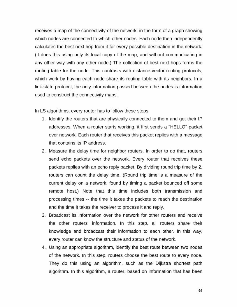
receives a map of the connectivity of the network, in the form of a graph showing

which nodes are connected to which other nodes. Each node then independently

calculates the best next hop from it for every possible destination in the network.

(It does this using only its local copy of the map, and without communicating in

any other way with any other node.) The collection of best next hops forms the

routing table for the node. This contrasts with distance-vector routing protocols,

which work by having each node share its routing table with its neighbors. In a

link-state protocol, the only information passed between the nodes is information

used to construct the connectivity maps.

In LS algorithms, every router has to follow these steps:

1. Identify the routers that are physically connected to them and get their IP

addresses. When a router starts working, it first sends a "HELLO" packet

over network. Each router that receives this packet replies with a message

that contains its IP address.

2. Measure the delay time for neighbor routers. In order to do that, routers

send echo packets over the network. Every router that receives these

packets replies with an echo reply packet. By dividing round trip time by 2,

routers can count the delay time. (Round trip time is a measure of the

current delay on a network, found by timing a packet bounced off some

remote host.) Note that this time includes both transmission and

processing times -- the time it takes the packets to reach the destination

and the time it takes the receiver to process it and reply.

3. Broadcast its information over the network for other routers and receive

the other routers' information. In this step, all routers share their

knowledge and broadcast their information to each other. In this way,

every router can know the structure and status of the network.

4. Using an appropriate algorithm, identify the best route between two nodes

of the network. In this step, routers choose the best route to every node.

They do this using an algorithm, such as the Dijkstra shortest path

algorithm. In this algorithm, a router, based on information that has been

34

collected from other routers, builds a graph of the network. This graph

shows the location of routers in the network and their links to each other.

Every link is labeled with a number called the weight or cost. This number

is a function of delay time, average traffic, and sometimes simply the

number of hops between nodes. For example, if there are two links

between a node and a destination, the router chooses the link with the

lowest weight.

Advantages and disadvantages of link-state routing The primary advantage of link-state routing is that it reacts more quickly, and in a

bounded amount of time, to connectivity changes. The primary disadvantage of

link-state routing is that it requires more storage and more computing to run than

does distance-vector routing.

Hierarchical Routing As you see, in both LS and DV algorithms, every router has to save some

information about other routers. When the network size grows, the number of

routers in the network increases. Here is a typical graph and routing table for A:

35

Destination Line Weight

A --- ---

B B 1

C C 1

D B 2

E B 3

F B 3

G B 4

H B 5

I C 5

J C 6

K C 5

L C 4

M C 4

N C 3

O C 4

P C 2

Q C 3

Network graph and A's routing table

Consequently, the size of routing tables increases, as well, and routers can't

handle network traffic as efficiently. We use hierarchical routing to overcome this

problem. Let's examine this subject with an example: We use DV algorithms to

find best routes between nodes. In the situation depicted below, every node of

the network has to save a routing table with 17 records.

36

In hierarchical routing, routers are classified in groups known as regions. Each

router has only the information about the routers in its own region and has no

information about routers in other regions. So routers just save one record in

their table for every other region. In this example, we have classified our network

into five regions (see below).

Destination Line Weight

A --- ---

B B 1

C C 1

Region 2 B 2

Region 3 C 2

Region 4 C 3

Region 5 C 4

Hierarchical routing

37

If A wants to send packets to any router in region 2 (D, E, F or G), it sends them

to B, and so on. As you can see, in this type of routing, the tables can be

summarized, so network efficiency improves. The above example shows two-

level hierarchical routing. We can also use three- or four-level hierarchical

routing. In three-level hierarchical routing, the network is classified into a number

of clusters. Each cluster is made up of a number of regions, and each region

contains a number or routers. Hierarchical routing is widely used in Internet

routing and makes use of several routing protocols.

6.5 Congestion Control In a network vulnerable to congestion, the more the total amount of sent packets

reaches the maximum capacity, the more the total amount of delivered packets

decreases. This can result in a situation where nearly no packets get delivered

successfully. The goal of congestion control is to keep network capacity at its

maximum level. The following factors responsible for congestion:

• Slow network links

• Shortage of buffer space

• Slow processors

Congestion Control in computer networks covers several mechanisms getting the

performance - capacity desirable one and thus prevent the network from

congestion. The generic term Congestion Control covers preventive as well as

reactive mechanisms.

Congestion Control: Congestion Control means to react on situations when the

network is congested.

Congestion Avoidance: Congestion Avoidance covers mechanisms to prevent

congestion from happening.

38

The term congestion always applies to network resources that are congested. A

network resource is congested, when the following condition is true:

Total Demand > Available Resources

Congestion Control can be realized by working on either side of the equation,

thus by decreasing demand or by increasing available resources. To control

congestion in computer networks, it is important to take a look on the architecture

and implementation of the network, because any design decision affects the

congestion control strategy of the network and thus the demand or the available

resources in the previous equation. Those design decisions are called Policies.

One important policy is the connection mechanism. There are two fundamental

distinct network types, connection-oriented and connectionless networks. In

connection-oriented network,all communication of a connection between two

endpoints is routed over the same gateways. In connectionless networks, single

packets are routed independently. Therefore, packets belonging to a single

connection can be routed differently.

Admission Control as described in below is part of the connection-oriented

networks concept, but it is conceptually not a part of connectionless networks.

However, state of the art network architectures combine the robustness of the

cheaper connectionless networks with the service quality advantages of

connection-oriented networks. The Quality of Service (QoS) research area deals

with this topic. Congestion Control and resource allocation are two sides of the

same coin.

In a congested network, where Total Demand > Available Resources is true.

It is often desirable to allocate the rare resources fair, so that every participant

gets an equal share of the networks capacity. Packet queuing and service

39

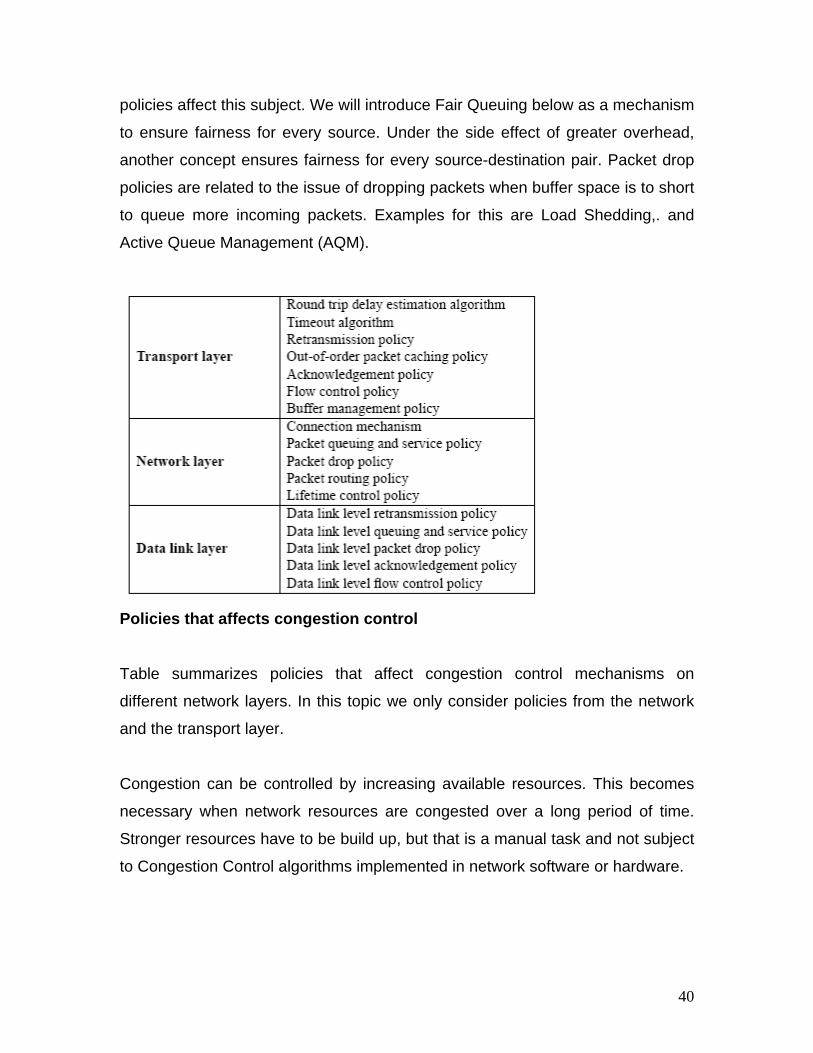
policies affect this subject. We will introduce Fair Queuing below as a mechanism

to ensure fairness for every source. Under the side effect of greater overhead,

another concept ensures fairness for every source-destination pair. Packet drop

policies are related to the issue of dropping packets when buffer space is to short

to queue more incoming packets. Examples for this are Load Shedding,. and

Active Queue Management (AQM).

Policies that affects congestion control

Table summarizes policies that affect congestion control mechanisms on

different network layers. In this topic we only consider policies from the network

and the transport layer.

Congestion can be controlled by increasing available resources. This becomes

necessary when network resources are congested over a long period of time.

Stronger resources have to be build up, but that is a manual task and not subject

to Congestion Control algorithms implemented in network software or hardware.

40

Three examples to increase available resources:

1. Dial-up links can be added during high usage.

2. Power increases on satellite links to increase their bandwidth.

3. Network paths can be split, so that extra traffic is sent via routes that may not

be considered as optimal under low load. This solution is not yet researched well

and therefore is not used in practice today. This approach breaks with the

concept of connection-oriented networks, because data is no longer routed over

e same network path.

service can be classified in various ways. The following classification

pproach:

drops. Open loop solutions do not take the actual network state into

ccount.

isms based on the

losed-loop use feedback mechanisms to control congestion.

n be distinguished:

ve congestion.

th

Here focus is on Congestion Control algorithms that decrease demand or

service. The mechanisms that try to handle congestion by degradation of

demand or

a

Open-loop Open-loop solutions for Congestion Control try to solve the problem

of congestion by a good design of themselves, thus a once started system does

not need to be modified because congestion does not occur anyway. Open loop

solutions also includes decisions about admission for connection establishment

or packet

a

Closed-loop In contrast to the open-loop solutions, mechan

c

Three steps necessary to control congestion ca

1. Observing the system to detect congestion.

2. Informing agents that are able to resol

3. Taking action to resolve the problem.

41

The Open-loop/Closed-loop classification of the Congestion Control mechanisms

oes not appear to be optimal in our case, because it only allows us to divide the

pre

The al

. The network layer on which the algorithms work according to the OSI/ISO

2. or

gateways as well as pairs or groups of them. To give a good introduction

ngestion Control research area, it is noted for each and every

eaks. Handling these traffic peaks is quite simple.

ontrolling the sending rate on network participants must flatten traffic peaks.

uality of service negotiation is

alled Traffic Policing. To control the sending rate of agents and prevent the

d

sented algorithms into two categories.

gorithms are categorized by two dimensions:

1

model. These can be transport or network layer as well as algorithms

working between these layers.

The involved network resources. Those can be single endpoints

into the Co

mechanism presented here, if it is an open- or a closed-loop solution.

Traffic Shaping All network nodes like hosts or gateways, can be sending agents, because they

are able to send data to other network nodes. In computer networks, one of the

main reasons for congestion is that data is not sent in constant rates but rather in

bursts called traffic p

C

This kind of traffic control is a preventive Congestion Avoidance mechanism

called Traffic Shaping.

In networks based on virtual circuits, the transmission rates and quality are

negotiated with receiving network nodes when a connection is initialized. A flow

specification is the result of this negotiation. Sending agents have to adhere to

the flow specification and shape their traffic accordingly. In packet switched

networks the volume of traffic is changing quickly over time. This makes periodic

renegotiations necessary in those networks. Q

c

42

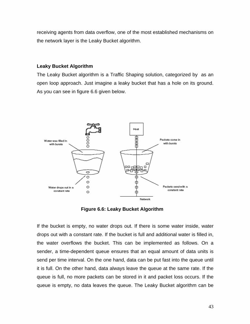
receiving agents from data overflow, one of the most established mechanisms on

Leaky Bucket Algorithm The Leaky Bucket algorithm is a Traffic Shaping solution, categorized by as an

open loop approach. Just imagine a leaky bucket that has a hole on its ground.

As you can see in figure 6.6 given below.

the network layer is the Leaky Bucket algorithm.

Figure 6.6: Leaky Bucket Algorithm

If the bucket is empty, no water drops out. If there is some water inside, water

drops out with a constant rate. If the bucket is full and additional water is filled in,

the water overflows the bucket. This can be implemented as follows. On a

sender, a time-dependent queue ensures that an equal amount of data units is

send per time interval. On the one hand, data can be put fast into the queue until

it is full. On the other hand, data always leave the queue at the same rate. If the

queue is full, no more packets can be stored in it and packet loss occurs. If the

ueue is empty, no data leaves the queue. The Leaky Bucket algorithm can be q

43

implemented for packets or a constant amount of bytes, send within each time

, also categorized as an open-loop approach. This algorithm

llows bursts for short transmission while making sure that no data is lost. In

m. In this

ituation, when an application sends a series of 100 data portions through the

e traffic shape is displayed on

iagram (c) in figure 6.7, where the sample incoming burst displayed on diagram

cket with a constant

interval. Using this algorithm, transmission peaks are flattened to a constant

transmission rate on a sending agent.

Token Bucket Algorithm A more flexible approach to control the sending rate on agents is the Token

Bucket algorithm

a

contrast to the Leaky Bucket algorithm, not the data that is to be send but tokens

are queued in a time-depended queue. One token is needed to send a single

portion of data.

Implementations contain a token counter that is incremented on every time

interval, so that the counter grows over time up until a maximum counter value is

reached. The token counter is decremented by one for every data portion sent.

When the token counter is zero, no data can be transmitted. An example would

be a token counter with a maximum of 50 tokens. When no data is sent for a

longer period of time, the counter will reach and stay at its maximu

s

network interface, 50 portions can be send immediately because there are 50

tokens available. After that, the remaining 50 portions are stored and transmitted

one by one on each time interval the token counter gets incremented.

Token Bucket’s characteristic influence on th

d

(a) is processed. First, there are enough buckets available to allow a burst over a

while. After that, the traffic is sent with a constant lower rate, because new

tokens get available at a constant rate of time.

Token Bucket as well as Leaky Bucket algorithms can be implemented for

packets or constant byte amounts. In the case of Token Bu

44

amount of bytes for each token, it is possible to store fractions of tokens for later

send a 50 byte packet, it is possible to

ol on gateways he algorithms in the previous section can work on every node in the network.

ribe some algorithms applied on routers or other gateways to

transmissions, when they have not be fully consumed by sending packets,. For

example when a 100 byte token is used to

store the rest of the token (50 bytes) for later transmissions.

Figure 6.7: Traffic Shaping with Leaky and Token Bucket Algorithms

Congestion ContrT

Now we will desc

avoid congestion.

Load Shedding An open-loop approach to control congestion on routers is the Load Shedding

mechanism. Load Shedding is a way to instruct a router to drop packets from its

queue, if it is congested. Note that the Load Shedding mechanism only reacts on

45

situations, where the router is already congested and no more packets can be

stored in the queue. Other queue management solutions like Active Queue

Management (AQM) to monitor the queue state and take actions to prevent the

router from congestion. When dropping packets, the router has to decide which

packets should be dropped. There are two concepts for dropping packets. On the

one hand the router can drop new incoming packets. This approach can be

optimal for file transmissions. Consider a router that has packets 7, 8 and 9 of a

10 packets long file in its full queue. Now packet 10 arrives. Assuming a

receiving host drops packets that arrive out of sequential order, the worst

decision would be to drop packet 7, as it would lead to retransmission of packets

7 to 10. Dropping packet 10 would be optimal, as it would be the only packet that

would have to be retransmitted. On the other hand for some multimedia and

realtime applications, the value of new packets is higher than the value of old

packets. In those cases the router can be instructed to drop old packets. The

oncept of dropping new packets is called wine, dropping old packets is called

plemented as tail-drop on queues, milk is implemented as head-

educe its data rates

ccording to congestion control algorithms will overflow the router and use more

or routers that misbehave do not use more resources and get

c

milk. Wine is im

drop.

Fair Queuing As they say Congestion Control and resource allocation are two sides of the

same coin. To enforce hosts and routers to implement and use congestion

control and avoidance algorithms described here, an open-loop mechanisms

called Fair Queuing was introduced. Imagine hosts and routers connected to a

router that reduces their data rates according to congestion control algorithms. A

connected misbehaving sending host that does not r

a

resources than well behaving hosts. To resolve this issue, a FIFO queue is

introduced on every incoming line as shown in figure 6.8.

Packets to deliver are chosen from all queues by a round robin algorithm. This

ensures, that hosts

46

a poorer service than they would, if they behaved well. Packets from

misbehaving hosts will be dropped when they overflow their incoming FIFO

queue on a router.

Figure 6.8: Fair Queuing Example Congestion Control between network nodes

his section shows some algorithms, working on the network layer between

fore communication is needed, that is not provided by the

ction-oriented networks. When a connection is

stablished, the connected endpoints can rely on the expected service quality, as

T

network nodes. There

IP protocol.

Admission Control Generally used in closed-loop, Congestion Avoidance mechanism is Admission

Control. Admission Control manages the establishment of connections between

connection endpoints in conne

e

congestion cannot occur. On the Internet, Admission Control cannot be applied

as it is working connectionless.

In connection-oriented networks, the transmissions belonging to a connection are

always routed over the same network nodes. When a host tries to establish a

connection, the virtual circuit has to be build up by all involved network nodes

that have the chance to decide, if theycan handle an additional connection or not.

Answering this kind of question is not trivial, since it requires the knowledge of

47

the current load on nodes as well as the expected additional load that results

from the additional connection. Clients must declare their demand of service

quality to aid this decision on the involved network nodes. For clients, this

approach seems to be a bit restrictive. However, it is a very stable solution. In

networks where connection establishment is only possible when the network load

allows it, clients get a guarantee that the requested quality of service is fulfilled

by the network. In such networks, there is no congestion during normal

operation. A problem is to ensure that all participants follow the policies they

advertised after the connections are established. If they use more service than

they requested, the network can be congested. In connection-oriented networks,

the network nodes have to save information about every connection, so it is

do not exceed their contracts. If not, they

xamples of connection-oriented networks using admission control to avoid

synchronous Transfer Mode (ATM)

possible for them to check, if clients

should decrease their service to the bad-behaving clients accordingly.

Figure 6.9: Admission control in computer networks

E

congestion are telephone networks or A

networks. As Figure 6.9 shows admission control in computer networks.

Resource Reservation Protocol (RSVP)

48

On the connectionless working internet, based on the IP protocol, some

application require a certainty about the Quality of Service (QoS) they get from

the network. A video stream, for example, needs a constant data rate as well as

constant delivery time of packets. The Resource reSerVation Protocol (RSVP) is

an extension protocol, conceptually working on the network layer that allows

clients to reserve resource on the network path for later transmission of data and

thus it is often used for multicast applications, but it can also be used in unicast

scenarios. RSVP is used by receiving hosts of downstream-only simplex

connections to reserve network resources along the route. Unicast connections

are one to one connections where multicast connections can be either one to

any or many to many connections. Multicast is a method to optimize traffic

ute. This minimizes network traffic in contrast to one to

ne connections. The routes are shaped as trees with the sending host as the

if the router has got enough capacity to

e

router does not have a reservation for the same stream yet, he must issue an

m

volume for scenarios where senders must send the same data to many

receivers.

In these scenarios, every router along the path can forward a single stream to

many receiving clients. This ensures that the data is transmitted only once along

every sender-receiver ro

o

root of the tree, routers being internal nodes and the leafs being receiving clients.

RSVP works as follows:

• When a client wants to establish a connection, it first issues an RSVP service

request in the upstream direction.

• The first router checks, if the requested service quality can be provided. The

requested service can be provided

forward a stream to the receiver. If not, the router sends a negative

acknowledgement to the receiver. If yes, the router must distinguish multicast

and unicast cases as described next.

• In multicast scenarios, a router must check if he has already got a reservation

for the same stream. If yes, he can signal free admission to the sender. If th

49

RSVP request to the next router on the route to the sender. If this RSVP request

is positively acknowledged, the router sends an acknowledgement to the client.

• In unicast scenarios, a router must always issue a new RSVP request in

quickly over time,

is reservation process must be repeated in intervals. When the client does not

rvation for a while, the reservation times out.

dy congested. In IP-based

etworks there is a possibility to send Choke Packets via Internet Control

ce quench messages.

tion on the congested resource more

uickly, all network nodes along the path should interpret and react immediately

at passes their way.

direction of the sender. If this RSVP request is positively acknowledged, the

router sends an acknowledgement to the client.

• Every router on the route works the same as the first router being contacted by

the receiving client. As internet traffic volume is changing very

th

re-request a rese

Choke Packets Choke Packets are a closed-loop solution that is used to directly inform a

sending host about congestion on a network resource along the network path.

The receiver should then take action to reduce load. When deciding about

issuing Choke Packets, relevant resources must be monitored. It is also

important not to issue too many choke packets, to give the receiver the chance to

react. Sending of Choke Packets is often criticized because additional packets

may increase the problem when the network is alrea

n

Message Protocol (ICMP) sour

Hop-by-Hop Choke Packets One problem with Choke Packets that are addressed to a sending host is the

long time that it takes to resolve the congestion. When the Choke Packet is

issued, there may be still a lot of packets on the way from the sender to the

congested resource. To resolve the situa

q

on a Choke Packet th

6.6 Summary

50

The network layer provides services to the transport layer. It can be based on

either virtual circuits or datagrams. In both cases, its main job is routing packets

from the source to the destination. In virtual-circuit subnets, a routing decision is

made when the virtual circuit is set up. In datagram subnets, it is made on every

packet. Many routing algorithms are used in computer networks. Static

algorithms include shortest path routing and flooding. Dynamic algorithms include

distance vector routing and link state routing. Most actual networks use one of

these. Subnets can easily become congested, increasing the delay and lowering

the throughput for packets. Network designers attempt to avoid congestion by

proper design. Networks differ in various ways, so when multiple networks are

interconnected problems can occur. Sometimes the problems can be finessed by

tunneling a packet through a hostile network, but if the source and destination

etworks are different, this approach fails. Protocols described are IP, a new

6.7

1. le of computer applications for which connection-oriented

service is appropriate. Now give two examples for which connectionless

2.

about the cube root of 4800 (around 16). Use trial and error to check out

3.

n

version of IP i.e. IPv6.

Self Assessment Questions

Give two examp

service is best.

For hierarchical routing with 4800 routers, what region and cluster sizes

should be chosen to minimize the size of the routing table for a three-layer

hierarchy? A good starting place is the hypothesis that a solution with k

clusters of k regions of k routers is close to optimal, which means that k is

combinations where all three parameters are in the general vicinity of 16.

A datagram subnet allows routers to drop packets whenever they are

needed to. The probability of a router discarding a packet is p. Consider

the case of a source host connected to the source router, which is

51

connected to the destination router, and then to the destination host. If

either of the routers discards a packet, the source host eventually times

out er-router lines are counted

as

n?

. transmissions a packet makes?

. Give an argument why the leaky bucket algorithm should allow just one

5.

4-byte packet, or two 512-byte

packets, etc., may be sent on each tick. Give a serious restriction of this

6. . The

token bucket is filled at a rate of 1 Mbps. It is initially filled to capacity with

7.

c, a token bucket size of 1

million bytes, and a maximum transmission rate of 50 million bytes/sec.

9. IPv6 uses 16-byte addresses. If a block of 1 million addresses is allocated

and tries again. If both host-router and rout

hops, what is the mean number of

a. hops a packet makes per transmissio

b

c. hops required per received packet?

4

packet per tick, independent of how large the packet is.

The byte-counting variant of the leaky bucket algorithm is used in a

particular system. The rule is that one 102

system that was not mentioned in the text.

A computer on a 6-Mbps network is regulated by a token bucket

8 megabits. How long can the computer transmit at the full 6 Mbps?

Imagine a flow specification that has a maximum packet size of 1000

bytes, a token bucket rate of 10 million bytes/se

How long can a burst at maximum speed last?

8. Describe a way to reassemble IP fragments at the destination.

every picosecond, how long will the addresses last?

52

10. The Protocol field used in the IPv4 header is not present in the fixed IPv6

header. Explain why?

6.8 Referenc

um,

PHI / Pearson’s Publications

• Computer Networks (2nd edition), Uyless Black, PHI Publication

• Computer Network, ED Tittle, Tata MacGraw Hills Publications

es / Suggested Readings

• Computer Networks (3rd & 4th Edition), Andrew S. Tannenba

53

Lesson No.: 7 Author: Mr. Yudhvir Singh

Title of the Lesson: Transport Layer Protocols Vetter: Dr. Manoj Dhun

Structure 7.0 Objective 7.1 Introduction

7.2 Services

7.3 Elements of Transport Protocols

7.4 User Datagram Protocol (UDP)

7.5 Transmission Control Protocol (TCP)

7.6 Summary

7.7 Self Assessment Questions

7.8 References / Suggested Readings

7.0 Objective In this lesson we will study the design principles for layer 4, the transport layer. This

study deals with the services, design, and elements protocols for achieving reliable,

efficient communication between two adjacent machines/peers at the transport layer.

Protocols discussed are UDP, TCP, connection management etc.

7.1 Introduction

Protocols at the transport layer oversee the delivery of data from a process (a running

application program) on one computer to a process on another computer. These

transport layer protocols act as liaison or interface between the application layer

protocols and the services provided by lower layers (network, data link, and physical).

The application layer programs interact with each other, using the services of the

transport layer, without even being aware of the existence of the lower layers. In effect,

the application layer programs are oblivious to the intricacies of the physical network

and are not dependent on the physical network type.

The figure 7.1 shows the position of the transport layer in the OSI model. The upper

three layers (application, transport, and session) have been grouped together as one

application layer, as in the Transmission Control Protocol/Internet Protocol (TCP/IP)

model. The transport layer receives services from the network layer and provides

services for the application layer:

Figure 7.1: Transport Layer in ISO-OSI Reference Model

The transport layer hides details of any network-dependent information from the

higher layers by providing transparent data transfer. The transport layer is concerned

with machine-to-machine transfer rather than process-to-process. The transport layer

will split data into smaller packets dispatch those packets and at the receiver

reassemble the data in the correct sequence.

7.2 Services The ultimate goal of the transport layer is to provide efficient, reliable, and cost-

effective service to its users, normally processes in the application layer. To achieve

this goal, the transport layer makes use of the services provided by the network layer.

The hardware and/or software within the transport layer that does the work is called

the transport entity. The transport entity can be located in the operating system kernel,

in a separate user process, in a library package bound into network applications, or

conceivably on the network interface card. The (logical) relationship of the network,

transport, and application layers is illustrated in figure 7.2.

igure 7.2: Logical – Relationship between network, transport and application layers

ust as there are two types of network service, connection-oriented and

onnectionless versus Connection-Oriented Service connection-oriented.

F

J

connectionless, there are also two types of transport services.

CA transport-layer protocol can be either connectionless or

Connectionless Service e, the packets are sent from one party to another with no

onnection-Oriented Service , a connection is first established between the sender

eliable versus Unreliable n be reliable or unreliable. If the application-layer protocol

.3 Elements of Transport Protocols

PDU (Transport Protocol Data Unit) for messages sent from transport entity to

In a connectionless servic

need for connection establishment or connection release. The packets are not

numbered, so they may be delayed, lost, or arrive out of sequence. There is no

acknowledgement either. One of the transport-layer protocols, User Datagram

Protocol (UDP), is connectionless.

CIn a connection-oriented service

and the receiver. Data are then transferred. At the end, the connection is released.

Transmission Control Protocol (TCP) is a connection-oriented service.

RThe transport-layer service ca

needs reliability, a reliable transport-layer protocol is used to implement flow and error

control. This means a slower and more complex service. However, if the application

program does not need reliability because it uses its own flow and error control

mechanism or if it needs fast service or the nature of the service does not demand flow

and error control (e.g. real time applications), an unreliable protocol can be used. There

are two different transport-layer protocols. UDP is connectionless and unreliable; TCP is

connection-oriented and reliable.

7 T

transport entity. Thus, TPDUs (exchanged by the transport layer) are contained in

packets (exchanged by the network layer) as shown in figure 7.3. In turn, packets are

contained in frames (exchanged by the data link layer). When a frame arrives, the

data link layer processes the frame header and passes the contents of the frame

payload field up to the network entity. The network entity processes the packet header

and passes the contents of the packet payload up to the transport entity.

Figure 7.3: Nesting of TPDUs, packets, and frames

he transport layer may provide the following services to the session layer:

he establishment and release of transport connections port service data units

igure 7.4: State diagram of Connection establishment & release.

T

TThis is done by means of transport addresses and trans

(TSDUs). Each session entity has a transport address associated with it and provide

connections between transport addresses. There may be more than one transport

connection between two endpoints. One transport connection may support more than

one session- entity.

F

A state diagram for connection establishment and release for these simple primitives

ata transfer is in accordance with the required quality of service. The transport layer

hree-way handshake Connection Establishment ides to begin sending with the

onnection Release f terminating a connection: asymmetric release and symmetric

is given in figure 7.4. Each transition is triggered by some event, either a primitive

executed by the local transport user or an incoming packet. For simplicity, we assume

here that each TPDU is separately acknowledged. We also assume that a symmetric

disconnection model is used, with the client going first. Please note that this model is

quite complicated.

D

attempts to provide the quality of service required by its associated session-entity

using the service provided by the network layer. To achieve these the transport layer

need to incorporate the following functions:

TThis establishment protocol does not require both s

same sequence number, so it can be used with synchronization methods other than

the global clock method. The normal setup procedure when a host 1 initiate is shown

in figure 7.5. Host 1 chooses a sequence number, x, and sends a CONNECTION

REQUEST TPDU containing it to host 2. Host 2 replies with an ACK TPDU

acknowledging x and announcing its own initial sequence number, y. Finally, host 1

acknowledges host 2's choice of an initial sequence number in the first data TPDU

that it sends.

CThere are two styles o

release. Asymmetric release is the way similar to the telephone system works: when

one party hangs up, the connection is broken. Symmetric release treats the

connection as two separate unidirectional connections and requires each one to be

released separately. Asymmetric release is abrupt and may result in data loss.

Symmetric release does the job when each process has a fixed amount of data to

send and clearly knows when it has sent it. In other situations, determining that all the

work has been done and the connection should be terminated is not so obvious.

Figure 7.5: Three protocol scenarios for establishing a connection using a

low Control and Buffering problem in the transport layer is the same as in the data

makes it impractical to implement the data link buffering strategy in the transport layer.

three-way handshake. CR denotes CONNECTION REQUEST. (a) Normal operation. (b) Old duplicate CONNECTION REQUEST appearing out of nowhere. (c) Duplicate CONNECTION REQUEST and duplicate ACK.

FIn some ways the flow control

link layer, but in other way it is different. The basic similarity is that in both layers a

sliding window or other scheme is needed on each connection to keep a fast

transmitter from overrunning slow receiver. The main difference is that a router usually

has relatively few lines, whereas a host has numerous connections. This difference

The subnet provides datagram service, the sending transport entity must also buffer.

The receiver knows that the sender buffers all TPDUs until they are acknowledged,

do the buffering, there still remains the question of

e buffer size. If most TPDUs are nearly the same size, it is natural to organize the

between source buffering and destination buffering depends on

e type of traffic carried by the connection. For low-bandwidth bursty traffic, such as

the receiver may or may not dedicate specific buffers to specific connections, as it

sees fit. The receiver may maintain a single buffer pool shared by all connections.

When a TPDU comes in, an attempt is made to dynamically acquire a new buffer. If

one is available, the TPDU is accepted; otherwise, it is discarded. Since the sender is

prepared to retransmit TPDUs lost by the subnet, having the receiver drop TPDUs,

although some resources are wasted, does no harm. The sender just keeps trying

until it gets an acknowledgement.

Even if the receiver has agreed to

th

buffers as a pool of identically sized buffers, with one TPDU per buffer. However, if

there is wide variation in TPDU size, from a few characters typed at a terminal to

thousands of characters from file transfers, a pool of fixed-sized buffers presents

problems. If the buffer size is chosen equal to the largest possible TPDU, space will

be wasted whenever a short TPDU arrives. If the buffer size is chosen less than the

maximum TPDU size, multiple buffers will be needed for long TPDUs, with the

attendant complexity.

The optimum trade-off

th

that produced by an interactive terminal, it is better not to dedicate any buffers, but

rather to acquire them dynamically at both ends. Since the sender cannot be sure the

receiver will be able to acquire a buffer, the sender must retain a copy of the TPDU

until it is acknowledged. On the other hand, for file transfer and other high-bandwidth

traffic, it is better if the receiver dedicate a full window of buffers, to flow the data at

maximum speed. Thus, for low-bandwidth bursty traffic, it is better to use buffer at the

sender end, and for high bandwidth smooth traffic, it is better to use buffer at the

receiver end.

Multiplexing Multiplexing is used for several conversations on one connection, virtual circuits, and

hysical links plays a role in several layers of the network architecture. If only one

ss is available on a host, all transport connections on that machine have

crashes, recovery from these crashes becomes an

sue. If the transport entity is entirely within the hosts, recovery from network and

traightforward. If the network layer provides datagram service, the

pped onto network addresses that identify the endpoints. One

ansport entity may serve more than one session entity and several transport

and a transport connection

ay be split between a numbers of different network connections.

p

network addre

to use it. When a TPDU comes, some way is needed to process it, the way for it to

process is given, this situation, called upward multiplexing. If a user needs more

bandwidth than one virtual circuit, a way out is to open multiple network connections

and to distribute the traffic among them on a round-robin basis; this modus operandi is

called downward multiplexing.

Crash Recovery If hosts and routers subject to

is

router crashes is s

transport entities expect lost TPDUs all the time and know how to cope with them. If

the network layer provides connection-oriented service, then loss of a virtual circuit is

handled by establishing a new one and then probing the remote transport entity to ask

it which TPDUs it has received and which ones it has not received. The latter ones

can be retransmitted.

Transport address to network address mapping: Transport connections are end-

to-end. These are ma

tr

addresses may be associated with one network address.

Multiplexing and splitting of transport connections: A number of transport

connections may be carried on one network connection

m

Also the layer will provide the following functions -

• Sequencing

• Flow Control

• Error detection and recover

Process-to-process delivery Process to process delivery is achieved through a set of functions performed by the

tran t are packetizing, connection control, addressing,

ties are shown in the figure 7.6:

sport layer. The most importan

and providing reliable. These du

Figure 7.6: Functions / Duties of Transport Layer

Packetizing: Packetizing divides a long message into smaller ones. These are then

encaps et and after that headers

re added.

riented and connectionless.

irtual path) between the sender and receiver.

The connection is virtual in that the application layer perceives that a single path

ently without any connection between them.

ulated into the data field of the transport-layer pack

a

Connection Control: Transport-layer protocols are divided into two categories:

connection-o

Connection-Oriented Delivery: A connection-oriented transport layer protocol

first establishes a connection (a v

has been created. In reality the packets may travel through different physical

paths. A session is said to exist between sender and receiver and the session

remains intact until broken by one of the parties. Once the session is established,

the two parties can send multiple packets related to each other, travelling one

after another through the virtual path. The packets may travel out of order, but

the transport layer ensures that this is transparent to the application program.

The packets are numbered consecutively and communication can take place in

both directions.

Connectionless Delivery: A connectionless transport protocol treats each

packet independ

Addressing: When an application process wishes to set up a connection to a remote

applica

used i en for connection

st, the client needs a

nique address of the remote computer and addressing is implemented at the network

t uses its services. Reliability involves flow control and error control.

er is

sponsible for delivery of datagrams between two hosts. This is called host-to-host

tion process, it must specify which one to connect to. The method normally

s to define transport addresses to which processes can list

requests. In the Internet, these end points are called ports. In Asynchronous Transfer

Mode (ATM) networks, they are called ATM adaptation Layer – Service Access Points

(AAL-SAPs). We will use the generic term TSAP, (Transport Service Access Point).

The analogous end points in the network layer are then called Network Service

Access Points (NSAPs). IP addresses are examples of NSAPs.

Consider, for example, that an HTTP client (a browser) on a local computer needs to

send a request to an HTTP server on a remote computer. Fir

u

layer. The remote computer may though be running several programs, such as HTTP,

SMTP, and TELNET, at the same time. When the request arrives at the remote

computer it must be delivered to the correct server program, in our example to the

HTTP server program. The packet carrying the request must therefore specify to

which server program the request must be delivered. The request packet must also

specify the client program that sends the packet and the server uses this when it

responds to the request. The reason for this is that the local computer might also be

running several clients, since most people usually open several client programs at the

same time.

Providing Reliability: The transport layer can provide reliability for the application

program tha

The data-link layer is responsible for delivery of frames between two neighboring

nodes over a link. This is called node-to-node delivery. The network lay

re

delivery. However, real communication on the Internet actually takes place between

two processes (application programs) and for this we need process-to-process

delivery. At any time there may be several processes running at both the source host

and the destination host. To complete the delivery, a mechanism is needed to deliver

data from one of the processes running on the source host to the corresponding

process running on the destination host. The transport layer is responsible for

process-to-process delivery, the delivery of a packet, part of a message, from one

process to another. Two processes communicate in a client-server relationship.

Figure 7.7: Deliveries Type and their Domains

The figure 7.7 shows the three types of deliveries and their domains:

lient-Server Paradigm munication, the

ost common one is through the client-server paradigm. A process on the local host,

vices from a process usually on a remote host, called a

st

cess

AddreWhenever something needs to be delivered to one specific address amongst many an

address is needed. At the data link layer, a MAC address is needed to choose between

CAlthough there are several ways to achieve process-to-process com

m

called a client, needs ser

server. A remote computer can run several server programs simultaneously as can a

local computer can run several client programs. For communication, the following are

therefore defined:

• Local host

• Local process

• Remote ho

• Remote pro

ssing

nodes. A frame in the data link layer needs a destination MAC address for delivery and a

source MAC address for the next node’s reply. At the network layer, an IP address is

needed to choose one host from among millions. A datagram in the network layer needs a

destination IP address for delivery and a source IP address for the destination’s reply. At

the transport layer, a transport-layer address is needed, called a port number, to choose

among multiple processes running on the destination host. The destination port number is

needed for delivery and the source port number is needed for the reply. In TCP/IP, port

numbers are 16-bit integers between 0 and 65,535. The client program defines itself with a

port number, chosen randomly by the transport layer software running on the client host.

This is the ephemeral port number. The server program must also define itself a port

number, but this cannot be chosen randomly. The Internet has decided to use universal

port numbers for servers, called well-know port numbers. Every client knows the well-

known port number of the corresponding server process. Consider an example of a

Daytime client process running on a local host and a Daytime server process running on a

remote host. The Daytime client process can use an ephemeral (temporary) port number

52,000 to identify itself and the daytime server process must use the well-know port

number 13. The figure 7.8 illustrates this concept:

Figure 7.8: Addressing at Transport Layer

IP addresses and port addresses play different roles in selecting the final destination

of data. The g the different hosts in the

orld. After the host has been selected, the port number defines one of the processes

on this particular host. This is illustrated in the figure 7.9:

destination IP address defines the host amon

w

Figure 7.9 IP & Port Addressing Concept

IANA Ranges The IANA (Internet Assigned Number Authority) has divided the port numbers into

three r (or private), as show in the figure

.10:

anges: well known, registered, and dynamic

7

Figure 7.10: IANA Ranges for Port Numbers.

Socket Addresses Process-to-process delivery needs two identifiers, IP address and the port number, at

ach end-to-e ss and a port number is

alled a socket address. The client socket address defines the client process uniquely

ket address defines the server process uniquely as shown in figure

7.11.

nd connection. The combination of an IP addre

c

just as the server soc

Figure 7.11: Socket Addressing

A transport layer protocol needs a pair of socket addresses: the client socket address

and the server socket address. These four pieces of information are part of the IP

header and the transport-layer protocol header. The IP header contains the IP

address and e port number.

does not add anything

the services of IP except for providing process-to-process communication instead of

-to forms very little error checking. UDP is a very

imple protocol with a minimum of overhead. If a process wants to send a small

es.

the UDP or TCP header contains th

7.4 User Datagram Protocol (UDP) The simple unreliable transport layer protocol is called the User Datagram Protocol

(UDP). UDP is a connectionless, unreliable transport protocol. It

to

host -host communication. Also, it per

s

message and does not care much about reliability, it can use UDP. Sending a small

message using UDP takes much less time than using TCP. In addition, UDP is a

convenient protocol for multimedia and multicasting applications.

The service provided by UDP is an unreliable service that provides no guarantees for

delivery and no protection from duplication (e.g. if this arises due to software errors

within an Intermediate System (IS)). The simplicity of UDP reduces the overhead from

using the protocol and the services may be adequate in many cas

A computer may send UDP packets without first establishing a connection to the

recipient. The computer completes the appropriate fields in the UDP header (PCI) and

forwards the data together with the header for transmission by the IP network layer as

shown in figure 7.12.

Figure 7.12: UDP Header

The UDP protocol header consists of 8 bytes of Protocol Control Information (PCI)

The UDP header consists of four fields each of 2 bytes in length:

ckets from a client use this as a service access point (SAP)

to indicate the session on the local client that originated the packet. UDP packets

• Destination Port (UDP packets from a client use this as a service access point

er. UDP packets from

•

checksum is the Standard Internet

ta is not checked by the receiver.)

Like fo

Interm

the sam

receive

• Source Port (UDP pa

from a server carry the server SAP in this field)

(SAP) to indicate the service required from the remote serv

a server carry the client SAP in this field)

UDP length (The number of bytes comprising the combined UDP header

information and payload data)

• UDP Checksum (A checksum to verify that the end to end data has not been

corrupted by routers or bridges in the network or by the processing in an end

system. The algorithm to compute the

Checksum algorithm. If this check is not required, the value of 0x0000 is placed

in this field, in which case the da

r other transport protocols, the UDP header and data are not processed by

ediate Systems (IS) in the network, and are delivered to the final destination in

e form as originally transmitted. At the final destination, the UDP protocol layer

s packets from the IP network layer as shown in figure 7.13.

Figure 7.13: Packet Transmission – UDP at Transport Layer These are checked using the checksum (when >0, this checks correct end-to-end

operation of the network service) and all invalid PDUs are discarded. UDP does not

make any provision for error reporting if the packets are not delivered. Valid data are

by the source and

estination port numbers (i.e. the session service access points).

tion port of packets

ent by the client is usually set to one of a number of well-known ports. These usually

received IP source address and the received

nique UDP source port number. Any responses which the server needs to send to

passed to the appropriate session layer protocol identified

d

Generally, clients set the source port number to a unique number that they choose

themselves - usually based on the program that started the connection. Since this

number is returned by the server in response, this lets the sender know which

"conversation" incoming packets are to be sent to. The destina

s

correspond to one of a number of different applications, e.g. port 23 is used for telnet,

and port 80 is used for web servers.

A server process (program), listens for UDP packets received with a particular well-

known port number and tells its local UDP layer to send packets matching this

destination port number to the server program. It determines which client these

packets come from by examining the

u

back to a client are sent with the source port number of the server (the well-known

port number) and the destination port selected by the client.

UDP uses port numbers as the addressing mechanism in the transport layer. Some

well-known port numbers used by UDP are listed in table 7.1.

Port Protoc

Table 7.1: Well-known ports for UDP Protocols User Datagram UDP packets are also called user datagrams.

DP is used by applications such as Trivial File Transfer Protocol (TFTP) since this

es flow and error control.

Applications U

application includ

7.5 Transmission Control Protocol (TCP)

ol

nection-oriented and reliable transmission

rotocol. It adds connection-oriented and reliability features to IP. TCP applies to the

hysical and link layers to handle error control, encryption or flow control you

iver.

ongestion control defines the methods for implicitly interpreting signals from the

nderlying packet

witched network provide formidable challenges for managers, designers and

The reliable, but complex transport-layer protocol is called Transmission Contr

Protocol (TCP). TCP is called a stream con

p

Internet, the end-to-end argument says that by putting excessive intelligence in

p

unnecessarily complicate the system. This is because these functions will usually

need to be done at the endpoints anyway, so why duplicate the effort along the way?

The result of an end-to-end network then, is to provide minimal functionality on a hop-

by-hop basis and maximal control between end-to-end communicating systems.

The end-to-end argument helped determine how the characteristics of TCP operate;

performance and error handling. TCP performance is often dependent on a subset of

algorithms and techniques such as flow control and congestion control. Flow control

determines the rate at which data is transmitted between a sender and rece

C

network in order for a sender to adjust its rate of transmission. The term congestion

control is a bit of a misnomer. Congestion avoidance would be a better term since

TCP cannot control congestion per se. Ultimately intermediate devices, such as IP

routers would only be able to control congestion. Congestion control is currently a

large area of research and concern in the network community. A companion study on

congestion control examines the current state of activity in that area.

Timeouts and retransmissions handle error control in TCP. Although delay could be

substantial, particularly if you were to implement real-time applications, the use of both

techniques offer error detection and error correction thereby guaranteeing that data

will eventually be sent successfully. The nature of TCP and the u

s

researchers of networks. Once regulated to low speed data communication

applications, the Internet and in part TCP are being used to support very high speed

communications of voice, video and data. It is unlikely that the Internet protocols will

remain static as the applications change and expand. Understanding the current state

of affairs will assist us in understanding protocol changes made to support future

applications.

Transmission Control Protocol TCP is often described as a byte stream, connection-oriented, reliable delivery transpo

layer protocol. In turn, we will discuss the meaning for each of these descriptive terms.

rt

yte Stream Delivery ication layer above and the network layer below.

manageable pieces to the receiver. It is this lack of 'record boundaries" which give it

elivery service".

hecksums: All TCP segments carry a checksum, which is used by the receiver to

with either the TCP header or data.

n: It is possible for packets to be duplicated in packet

witched network; therefore TCP keeps track of bytes received in order to discard

etransmissions: In order to guaranteed delivery of data, TCP must implement

retransmission schemes for data that may be lost or damaged. The use of positive

BTCP interfaces between the appl

When an application sends data to TCP, it does so in 8-bit byte streams. It is then up

to the sending TCP to segment or delineate the byte stream in order to transmit data

in

the name "byte stream d

Connection-Oriented Before the two communicating TCPs exchange data, they must first agree upon the

willingness to communicate. Analogous to a telephone call, a connection must first be

made before two parties exchange information.

Reliability A number of mechanisms help provide the reliability TCP guarantees. Each of these is

described briefly below. Cdetect errors

Duplicate data detectios

duplicate copies of data that has already been received.2

R

acknowledgements by the receiver to the sender confirms successful reception of

data. The lack of positive acknowledgements, coupled with a timeout period (see

timers below) calls for a retransmission.

Sequencing: In packet switched networks, it is possible for packets to be delivered

out of order. It is TCP's job to properly sequence segments; it receives, so that it can

deliver the byte stream data to an application in order.

Timers: TCP maintains various static and dynamic timers on data sent. The sending

CP waits for the receiver to reply with an acknowledgement within a bounded length

CP Header Format

T

of time. If the timer expires before receiving an acknowledgement, the sender can

retransmit the segment.

TRemember that the combination of TCP header and TCP in one packet is called a TCP

segment.

Figure 7.14: TCP Header Format

Figure 7.14 depicts the format of all valid TCP segments. The size of the header without

options is 20 bytes. We will briefly define each field of the TCP header in figure 7.14.

Source Port A 16-bit num CP segment originated

from within the sending host. The port numbers are divided into three ranges, well-

e

pplication layer. For example, the TELNET server is always assigned to the well-

ber identifying the application the T

known ports (0 through 1023), registered ports (1024 through 49151) and private ports

(49152 through 65535). Port assignments are used by TCP as an interface to th

a

known port 23 by default on TCP hosts. A complete pair of IP addresses (source and

destination) plus a complete pair of TCP ports (source and destination) define a single

TCP connection that is globally unique as given in table 7.2.

Table 7.2: Some ports for TCP Protocols

Destination Port is a 16-bit number, identifying the application the TCP segment. It is

destined for on a receiving host. Destination ports use the same port number

assignments as those set aside for source ports.

equence Number is a 32-bit number, identifying the current position of the first data

byte in the segment within the entire byte stream for the TCP connection. After

reaching 232 -1, this number will wrap around to 0.

S

Acknowledgement Number is a 32-bit number, identifying the next data byte the

sender expects from the receiver. Therefore, the number will be one greater than the

most recently received data byte. This field is only used when the ACK control bit is

rned on.

ithout options, a TCP header is

monly used.

). If this bit field is set, the acknowledgement field described

arlier is valid.

ush Function (PSH). If this bit field is set, the receiver should deliver this segment

plication, which can jump ahead of queued data.

eset the Connection (RST). If this bit is present, it signals the receiver that the

e freely relinquished.

tu

Header Length is a 4-bit field that specifies the total TCP header length in 32-bit

words (or in multiples of 4 bytes if you prefer). W

always 20 bytes in length. The largest a TCP header may be is 60 bytes. This field is

required because the size of the options field(s) cannot be determined in advance.

Note that this field is called "data offset" in the official TCP standard, but header length

is more com

Reserved is a 6-bit field currently unused and reserved for future use.

Control Bits Urgent Pointer (URG). If this bit field is set, the receiving TCP should

interpret the urgent pointer field.

Acknowledgement (ACKe

Pto the receiving application as soon as possible. An example of its use may be to send

a Control-BREAK request to an ap

R

sender is aborting the connection and all queued data and allocated buffers for the

connection can b

Synchronize (SYN). When present, this bit field signifies that sender is attempting to

"synchronize" sequence numbers. This bit is used during the initial stages of

connection establishment between a sender and receiver.

No More Data from Sender/Final (FIN). If set, this bit field tells the receiver that the

sender has reached the end of its byte stream for the current TCP connection.

Window A 16-bit integer used by TCP for flow control in the form of a data

sed to make use of even

rger windows.

TCP

eader and data fields. This 16-bit value will be compared with the value the receiver

of urgent data that should be processed by the receiving application

s soon as possible. This 16-bit field tells the receiver when the last byte of urgent

iver. Depending on the option(s) used, the

ngth of this field will vary in size, but it cannot be larger than 40 bytes due to the size

gestion control techniques.

transmission window size. This number tells the sender how much data the receiver is

willing to accept. The maximum value for this field would limit the window size to

65,535 bytes, however a "window scale" option can be u

la

Checksum A TCP sender computes a value based on the contents of the

h

generates using the same computation. If the values match, the receiver can be very

confident that the segment arrived intact.

Urgent Pointer In certain circumstances, it may be necessary for a TCP sender to

notify the receiver

a

data in the segment ends.

Options In order to provide additional functionality, several optional parameters may

be used between a TCP sender and rece

le

of the header length field (4 bits). The most common option is the maximum segment

size (MSS) option. A TCP receiver tells the TCP sender the maximum segment size it

is willing to accept through the use of this option. Other options are often used for

various flow control and con

Padding as the options may vary in size, it may be necessary to "pad" the TCP

header with zeroes so that the segment ends on a 32-bit word boundary as defined by

the standard.

Data may not used in some circumstances (e.g. acknowledgement segments with no

data in the reverse direction), this variable length field carries the application data from

CP sender to receiver. This field coupled with the TCP header fields constitutes a

tablishment and Termination CP provides a connection-oriented service over packet switched networks.

hree-Way Handshake g TCP they must first establish a

T

TCP segment.

Connection EsT

Connection-oriented implies that there is a virtual connection between two endpoints.

There are three phases in any virtual connection. These are the connection

establishment, data transfer and connection termination phases.

TIn order for two hosts to communicate usin

connection by exchanging messages in what is known as the three-way handshake.

The figure 7.15 depicts the process of the three-way handshake.

Figure 7.15 - TCP Connection Establishment

From figure 7.15, it can be seen that there are three TCP segments exchanged

between two hosts, host A and host B. Reading down the diagram depicts events in

time. To start, host A, initiates the connection by sending a TCP segment with the

SYN control bit set and an initial sequence number (ISN), we represent as the variable

x in the sequence number field.

At some moment later in time, host B, receives this SYN segment, processes it and

responds with a TCP segment of its own. The response from Host B contains the SYN

control bit set and its own ISN represented as variable y. Host B also sets the ACK

control bit to indicate the next expected byte from Host A should contain data starting

with sequence number x+1. When Host A receives Host B's ISN and ACK, it finishes

the connection establishment phase by sending a final acknowledgement segment to

Host B. In this case, Host A sets the AC

edgement number y+1 in the acknowledgement

" which determines how many bytes the

duplicated or lost, a "hole" may exist in

the byte stream. A receiver will continue to acknowledge the most current contiguous

K control bit and indicates the next expected

byte from Host B by placing acknowl

field.

In addition to the information shown in the figure above, an exchange of source and

destination ports to use for this connection are also included in each senders'

segments.

Data Transfer Once ISNs have been exchanged, communicating applications can transmit data

between each other. Most of the discussion surrounding data transfer requires us to

look at flow control and congestion control techniques

A simple TCP implementation will place segments into the network for a receiver as

long as there is data to send and as long as the sender does not exceed the window

advertised by the receiver. As the receiver accepts and processes TCP segments, it

sends back positive acknowledgements, indicating where is the byte stream. These

acknowledgements also contain the "window

receiver is currently willing to accept. If data is

place in the byte stream it has accepted. If there is no data to send, the sending TCP

will simply sit idly by waiting for the application to put data into the byte stream or to

receive data from the other end of the connection.

by the sender reaches a point where data sent will exceed the

nd unresponsive connections.

Delayed transmissions are used to make more efficient use of network bandwidth by

nd the network. It is important for

the transmission to be at a high enough rate to ensure good performance, but also to

ns today.

If data queued

receiver's advertised window size, the sender must halt transmission and wait for

further acknowledgements and an advertised window size that is greater than zero

before resuming. Timers are used to avoid deadlock a

sending larger "chunks" of data at once rather than in smaller individual pieces.

Connection Termination In order for a connection to be released, four segments are required to completely

close a connection. Four segments are necessary due to the fact that TCP is a full-

duplex protocol, meaning that each end must shut down independently.

Sliding Window and Flow Control Flow control is a technique whose primary purpose is to properly match the

transmission rate of sender to that of the receiver a

protect against overwhelming the network or receiving host. We note that flow control

is not the same as congestion control. Congestion control is primarily concerned with

a sustained overload of network intermediate devices such as IP routers. TCP uses

the window field, briefly described previously, as the primary means for flow control.

During the data transfer phase, the window field is used to adjust the rate of flow of

the byte stream between communicating TCPs.

Congestion Control TCP congestion control and Internet traffic management issues in general is an active

area of research and experimentation. This final section is a very brief summary of the

standard congestion control algorithms widely used in TCP implementatio

Slow Start Slow Start, a requirement for TCP software implementations is a mechanism used by

the sender to control the transmission rate, otherwise known as sender-based flow

control. This is accomplished through the return rate of acknowledgements from the

receiver. In other words, the rate of acknowledgements returned by the receiver

determine the rate at which the sender can transmit data.

When a TCP connection first begins, the Slow Start algorithm initializes a congestion

window to one segment, which is the maximum segment size (MSS) initialized by the

receiver during the connection establishment phase. When acknowledgements are

turned by the receiver, the congestion window increases by one segment for each

urned. Thus, the sender can transmit the minimum of the

low Start is actually not very slow when the network is not congested and network

me is good. For example, the first successful transmission and

cur.

n and stay slow.

re

acknowledgement ret

congestion window and the advertised window of the receiver, which is simply called

the transmission window.

S

response ti

acknowledgement of a TCP segment increases the window to two segments. After

successful transmission of these two segments and acknowledgements completes,

the window is increased to four segments. Then eight segments, then sixteen

segments and so on, doubling from there on out up to the maximum window size

advertised by the receiver or until congestion finally does oc

Congestion Avoidance During the initial data transfer phase of a TCP connection the Slow Start algorithm is

used. However, there may be a point during Slow Start that the network is forced to

drop one or more packets due to overload or congestion. If this happens, congestion

avoidance is used to slow the transmission rate. However, Slow Start is used in

conjunction with congestion avoidance as the means to get the data transfer going

again so it doesn't slow dow

In the Congestion Avoidance algorithm a retransmission timer expiring or the

reception of duplicate ACKs can implicitly signal the sender that a network congestion

situation is occurring. The sender immediately sets its transmission window to one half

of the current window size (the minimum of the congestion window and the receiver's

advertised window size), but to at least two segments. If congestion was indicated by

a timeout, the congestion window is reset to one segment, which automatically puts

the sender into Slow Start mode. If congestion was indicated by duplicate ACKs, the

st retransmit and fast recovery algorithms are invoked. As data is received during

e congestion window is increased. However, Slow Start is

fa

Congestion Avoidance, th

only used up to the halfway point where congestion originally occurred. This halfway

point was recorded earlier as the new transmission window. After this halfway point,

the congestion window is increased by one segment for all segments in the

transmission window that are acknowledged. This mechanism will force the sender to

more slowly grow its transmission rate, as it will approach the point where congestion

had previously been detected.

Fast Retransmit When a duplicate ACK is received, the sender does not know, it is because that a

TCP segment was lost or simply that a segment was delayed and received out of

order at the receiver. If the receiver can re-order segments, it should not be long

before the receiver sends the latest expected acknowledgement. Typically no more

than one or two duplicate ACKs should be received when simple out of order

conditions exist. If however more than two duplicate ACKs are received by the sender,

it is a strong indication that at least one segment has been lost. The TCP sender will

assume enough time has lapsed for all segments to be properly re-ordered by the fact

that the receiver had enough time to send three duplicate ACKs. When three or more

duplicate ACKs are received, the sender does not even wait for a retransmission timer

to expire before retransmitting the segment (as indicated by the position of the

duplicate ACK in the byte stream). This process is called the Fast Retransmit

algorithm. Immediately following Fast Retransmit is the Fast Recovery algorithm.

Fast Recovery Since the Fast Retransmit algorithm is used when duplicate ACKs are being received,

the TCP sender has implicit knowledge that there is data still flowing to the receiver.

The reason is because duplicate ACKs can only be generated when a segment is

received. This is a strong indication that serious network congestion may not exist and

that the lost segment was a rare event. So instead of reducing the flow of data

abruptly by going all the way into Slow Start, the sender only enters Congestion

Avoidance mode.

Rather than start at a window of one segment as in Slow Start mode, the sender

resumes transmission with a larger window, incrementing as if in Congestion

Avoidance mode.

7.6 Summary The transport layer is the key to understanding layered protocols. It provides various

st important of which is an end-to-end, reliable, connection-oriented

manage connections and timers, and allocate and utilize credits.

he Internet has two main transport protocols: UDP and TCP.

1. Why does the maximum packet lifetime, T, have to be large enough to ensure

e packet but also its acknowledgements have vanished?

services, the mo

byte stream from sender to receiver. It is accessed through service primitives that

permit the establishment, use, and release of connections.

Transport protocols must be able to do connection management over unreliable

networks. Connection establishment is complicated by the existence of delayed

duplicate packets that can reappear at inopportune moments. It must handle all the

service primitives,

T

7.7 Self Assessment Questions

that not only th

2. Imagine that a two-way handshake rather than a three-way handshake were

used to set up connections. In other words, the third message was not required.

Are deadlocks now possible? Give an example or show that none exist.

3. Why does UDP exist? Would it not have been enough to just let user processes

erver responds with a

sequence of data packets containing different parts of the requested file. To

d delivery, client and server use a stop-and-wait

protocol. Ignoring the obvious performance issue, do you see a problem with

. Both UDP and TCP use port numbers to identify the destination entity when

ing data link layer overhead?

8.

send raw IP packets?

4. Consider a simple application-level protocol built on top of UDP that allows a

client to retrieve a file from a remote server residing at a well-known address.

The client first sends a request with file name, and the s

ensure reliability and sequence

this protocol? Think carefully about the possibility of processes crashing.

5

delivering a message. Give two reasons for why these protocols invented a

new abstract ID (port numbers), instead of using process IDs, which already

existed when these protocols were designed.

6. What is the total size of the minimum TCP MTU, including TCP and IP

overhead but not includ

7. Datagram fragmentation and reassembly are handled by IP and are invisible to

TCP. Does this mean that TCP does not have to worry about data arriving in

the wrong order?

A process on host 1 has been assigned port p, and a process on host 2 has

been assigned port q. Is it possible for there to be two or more TCP

connections between these two ports at the same time?

9. The maximum payload of a TCP segment is 65,495 bytes. Why was such a

strange number chosen?

7.8

• Computer Networks (3rd & 4th Edition), Andrew S. Tannenbaum, PHI /

etwork, ED Tittle, Tata MacGraw Hills Publications

References / Suggested Readings

Pearson’s Publications

• Computer Networks (2nd edition), Uyless Black, PHI Publication

• Computer N

Lesson No.: 8 Author: Mr. Yudhvir Singh

Lesson Title: ISDN and ATM Vetter: Dr. Manoj Dhun

Structure 8.0 Objective 8.1 ISDN

8.1.1 Introduction

8.1.2 ISDN Concept

8.1.3 Principles of ISDN

8.1.4 The User Interface

8.1.5 Objectives

8.1.6 Architecture

8.1.7 Standards

8.1.8 ISDN CHANNELS

8.1.9 USER ACCESS

8.1.10 ISDN Protocol Architecture

8.1.11 ISDN Connections

8.2 ATM

8.2.1 Introduction

8.2.2 ATM Overview - ATM Header and Payload

8.3 Summary

8.4 Self Assessment Questions

8.5 References / Suggested Readings

8.0 Objective

In this lesson we will study the basic concepts of Integrated Services Digital Networks

(ISDN) and Asynchronous Transfer Mode (ATM).

8.1 ISDN

8.1.1 Introduction

Rapid advances in computer and communication technologies have resulted in the

increasing merging of these two fields. The lines have blurred among computing,

switching, and digital transmission equipment, and the same digital techniques are

being used for data, voice, and image transmission. Merging and evolving technologies,

coupled with increasing demands for efficient and timely collection, processing, and

dissemination of information, are leading to the development of integrated systems that

transmit and process all types of data. The ultimate goal of this evolution is the

integrated services digital network (ISDN). The ISDN is intended to be a worldwide

public telecommunications network to replace existing public telecommunications

networks and deliver a wide variety of services. The ISDN is defined by the

standardization of user interfaces and is implemented as a set of digital switches and

paths supporting a broad range of traffic types and providing value-added processing

services.

8.1.2 ISDN Concept The concept of ISDN is best introduced by considering it from several different

viewpoints:

• Principles of ISDN

• The user interface

• Objectives

• Services

8.1.3 Principles of ISDN

Standards for ISDN have been defined by ITU-T (formerly CCITT. ISDN-related

standards, states the principles of ISDN from the point of view of CCITT. Let us look at

each of these points in turn:

• Support of voice and non-voice applications using a limited set of standardized

facilities.

• Support for switched and non-switched applications.

• Reliance on 64-kbps connections.

• Intelligence in the network.

• Layered protocol architecture.

• Variety of configurations.

8.1.4 The User Interface Figure 8.3 given below is a conceptual view of the lSDN from a user, or customer, point

of view. The user has access to the ISDN by means of a local interface to a "digital

pipe" of a certain bit rate. Pipes of various sizes are available to satisfy differing needs.

At any given point in time, the pipe to the user's premises has a fixed capacity, but the

traffic on the pipe may be a variable mix up to the capacity limit. Thus, a user may

access circuit-switched and packet-switched services, as well as other services, in a

dynamic mix of signal types and bit rates. To provide these services, the ISDN requires

rather complex control signals to instruct it how to sort out the time multiplexed data and

provide the required services. These control signals are also multiplexed onto the same

digital pipe.

Figure 8.3: Conceptual view of ISDN connections

An important aspect of the interface is that the user may, at any time, employ less than

the maximum capacity of the pipe, and will be charged according to the capacity used

rather than "connect time." This characteristic significantly diminishes the value of

current user design efforts that are geared to optimize circuit utilization by use of

concentrators, multiplexers, packet switches, and other line sharing arrangements.

8.1.5 Objectives Activities currently under way are leading to the development of a worldwide ISDN.

Certain common objectives are as given below:

Standardization. It is essential that a single set of ISDN standards be provided to

permit universal access and to permit the development of cost-effective equipment.

Transparency. The most important service to be provided is a transparent transmission

service, thereby permitting users to develop applications and protocols with the

confidence that they will not be affected by the underlying ISDN.

Separation of competitive functions. It must be possible to separate out functions

that could be provided competitively as opposed to those that are fundamentally part of

the ISDN. In many countries, a single, government-owned entity provides all services.

Some countries desire that certain enhanced services be offered competitively (e.g.,

videotex, electronic mail). Leased and switched services. The ISDN should provide dedicated point-to point

services as well as switched services, thereby allowing the user to optimize

implementation of switching and routing techniques.

Cost-related tariffs. The price for ISDN service should be related to cost, and should

be independent of the type of data being carried. One type of service should not be in

the position of subsidizing others.

Smooth migration. The conversion to ISDN will be gradual, and the evolving network

must coexist with existing equipment and services. Thus, ISDN interfaces should evolve

from current interfaces, and provide a migration path for users.

Multiplexed support. In addition to providing low-capacity support to individual users,

multiplexed support must be provided to accommodate user owned PBX and local

network equipment.

8.1.6 Architecture Figure 8.4 given below is a block diagram of ISDN. ISDN supports a new physical

connecter for users, a digital subscriber loop (link from end user to central or end office),

and modifications to all central office equipment. The area to which most attention has

been paid by standards organizations is that of user access. A common physical

interface has been defined to provide, in essence, a DTE-DCE connection. The same

interface should be usable for telephone, computer terminal, and video-tex terminal.

Protocols are needed for the exchange of control information between user device and

the network. Under the ISDN, one or two twisted pairs are used to provide a basic full-

duplex digital communications link. The digital central office connects the numerous

ISDN subscriber loop signals to the IDN.

FIGURE 8.4: Block diagram of ISDN functions.

8.1.7 Standards The development of ISDN is governed by a set of recommendations issued by ISDN,

called the I-series Recommendations. The characterization of ISDN contained in these

Recommendations is centered on three main areas:

1. The standardization of services offered to users, so as to enable services to be

internationally compatible.

2. The standardization of user-network interfaces, so as to enable terminal equipment to

be portable, and to assist in (1).

3. The standardization of ISDN capabilities to the degree necessary to allow user-

network and network-network interworking, and thus achieve (1) and (2).

The I-series Recommendations are broken up into six main groupings, labeled 1.100

through 1.600.

• 1.100 Series-General Concepts

• 1.200 Series-Service Capabilities

• 1.300 Series-Network Aspects

• 1.400 Series-User-Network Interfaces

Physical configurations.

Transmission rates.

Protocol specifications.

• 1.500 Series-Internetwork Interfaces

• 1.600 Series-Maintenance Principles

8.1.8 ISDN CHANNELS The digital pipe between the central office and the ISDN user is used to carry a number

of communication channels. The capacity of the pipe, and therefore the number of

channels carried, may vary from user to user. The transmission structure of any access

link is constructed from the following types of channels:

• B channel: 64 kbps

• D channel: 16 or 64 kbps

• H channel: 384(H0), 1536(H11), and 1920 (H12) kbps

The B channel is the basic user channel. It can be used to carry digital data, PCM-

encoded digital voice, or a mixture of lower-rate traffic, including digital data and

digitized voice encoded at a fraction of 64 kbps. In the case of mixed traffic, all traffic

must be destined for the same endpoint. Four kinds of connections can be set up over a

B channel:

Circuit-switched. This is equivalent to switched digital service available today. The

user places a call, and a circuit-switched connection is established with another network

user. An interesting feature is that call-establishment dialogue does not take place over

the B channel, but is done over the D, as explained below.

Packet-switched. The user is connected to a packet-switching node, and data are

exchanged with other users via X.25.

Frame mode. The user is connected to a frame relay node, and data are exchanged

with other users via LAPF.

Semipermanent. This is a connection to another user set up by prior arrangement, and

not requiring a call-establishment protocol; this is equivalent to a leased line.

The D channel serves two purposes. First, it carries signaling information to control

circuit-switched calls on associated B channels at the user interface. In addition, the D

channel may be used for packet-switching or low-speed telemetry at times when no

signaling information is waiting. The channel function are given in table 8.4

Table 8.4: ISDN Channel Functions

H channels are provided for user information at higher bit rates. The user may employ

such a channel as a high-speed trunk, or the channel may be subdivided according to

the user's own TDM scheme. Examples of applications include fast facsimile, video,

high-speed data, high-quality audio, and multiple information streams at lower data

rates.

These channel types are grouped into transmission structures that are offered as a

package to the user. The best-defined structures at this time are the basic channel

structure (basic access) and the primary channel structure (primary access), which are

depicted in Figure 8.5.

Figure 8.5: ISDN channel structure

Basic access consists of two full-duplex 64-kbps B channels and a full-duplex 16-kbps

D channel. The total bit rate, by simple arithmetic, is 144 kbps. However, framing,

synchronization, and other overhead bits bring the total bit rate on a basic access link to

192 kbps. Each frame of 48 bits includes 16 bits from each of the B channels and 4 bits

from the D channel.

The basic service is intended to meet the needs of most individual users, including

residential and very small offices. It allows the simultaneous use of voice and several

data applications, such as packet-switched access, a link to a central alarm service,

facsimile, videotex, and so on. These services could be accessed through a single

multifunction terminal or several separate terminals. In either case, a single physical

interface is provided. Most existing two-wire local loops can support this interface.

In some cases, one or both of the B channels remain unused; this results in a B+D or D

interface, rather than the 2B+D interface. However, to simplify the network

implementation, the data rate at the interface remains at 192 kbps. Nevertheless, for

those subscribers with more modest transmission requirements, there may be a cost

savings in using a reduced basic interface.

Primary access is intended for users with greater capacity requirements, such as offices

with a digital PBX or a local network. Because of differences in the digital transmission

hierarchies used in different countries, it was not possible to get agreement on a single

data rate. The primary interface may also be used to support H channels. Some of

these structures include a 64-kbps D channel for control signaling. When no D channel

is present, it is assumed that a D channel on another primary interface at the same

subscriber location will provide any required signaling. The following structures are

recognized:

Primary rate interface HO channel structures. This interface supports multiple 384-

kbps HO channels. The structures are 3H0 + D and 4H0 for the 1.544-Mbps interface,

and 5H0 + D for the 2.048-Mbps interface.

Primary rate interface H1 channel structures. The HI1 channel structure consists of

one 1536-kbps HI1 channel. The H12 channel structure consists of one 1920-kbps H12

channel and one D channel.

Primary rate interface structures for mixtures of B and HO channels. This interface

consists of 0 or 1 D channels plus any possible combination of B and HO channels, up

to the capacity of the physical interface (e.g., 3H0 + 5B + D and 3H0 + 6B).

8.1.9 USER ACCESS To define the requirements for ISDN user access, an understanding of the anticipated

configuration of user premises equipment and of the necessary standard interfaces is

critical. The first step is to group functions that may exist on the user's premises.

Functional groupings. Certain finite arrangements of physical equipment or

combinations of equipment.

Reference points. Conceptual points used to separate groups of functions.

The architecture on the subscriber's premises is broken up functionally into groupings

separated by reference points. This separation permits interface standards to be

developed at each reference point; this effectively organizes the standards work and

provides guidance to the equipment providers. Once stable interface standards exist,

technical improvements on either side of an interface can be made without impacting

adjacent functional groupings. Finally, with stable interfaces, the subscriber is free to

procure equipment from different suppliers for the various functional groupings, so long

as the equipment conforms to the relevant interface standards.

Network termination I (NT1) includes functions associated with the physical and

electrical termination of the ISDN on the user's premises; these correspond to OSI

layer1.

Network termination 2 (NT2) is an intelligent device that can perform switching and

concentration functions; it may include functionality up through layer 3 of the OSI model.

Network termination 1, 2 (NT12) is a single piece of equipment that contains the

combined functions of NT1 and NT2; this points out one of the regulatory issues

associated with ISDN interface development.

Terminal equipment type I (TE1) refers to devices that support the standard ISDN

interface. Examples are digital telephones, integrated voice-data terminals, and digital

facsimile equipment. Terminal equipment type 2 (TE2) encompasses existing non-ISDN

equipment.

Reference point T (terminal) corresponds to a minimal ISDN network termination at

the customer's premises; it separates the network provider's equipment from the user's

equipment.

Reference point S (system) corresponds to the interface of individual ISDN terminals

and separates user terminal equipment from network-related communications functions.

Reference point R (rate) provides a non-ISDN interface between user equipment that

is not ISDN-compatible and adapter equipment.

8.1.10 ISDN Protocol Architecture Figure 8.6 illustrates, in the context of the OSI model, the protocols defined or

referenced in the ISDN documents. As a network, ISDN is essentially unconcerned with

user layers 4-7. These are end-to-end layers employed by the user for the exchange of

information. Network access is concerned only with layers 1-3. Layer 1, specifies the

physical interface for both basic and primary access. Because B and D channels are

multiplexed over the same physical interface, these standards apply to both types of

channels. Above this layer, the protocol structure differs for the two channels.

Figure 8.6: ISDN protocol at the user-network interface

For the D channel, a new data link layer standard, LAPD (Link Access Protocol, D

channel) has been defined. This standard is based on HDLC, modified to meet ISDN

requirements. All transmission on the D channel is in the form of LAPD frames that are

exchanged between the subscriber equipment and an ISDN switching element. Three

applications are supported: control signaling, packet switching, and telemetry. For

control signaling, a call control protocol has been defined. This protocol is used to

establish, maintain, and terminate connections on B channels; thus, it is a protocol

between the user and the network. Above layer 3, there is the possibility for higher-layer

functions associated with user-to-user control signaling.

The D channel can also be used to provide packet-switching services to the subscriber.

In this case, the X.25 level-3 protocol is used, and X.25 packets are transmitted in

LAPD frames. The X.25 level-3 protocol is used to establish virtual circuits on the D

channel to other users and to exchange packetized data. The B channel can be used

for circuit switching, semipermanent circuits, and packet switching. For circuit switching,

a circuit is set up on a B channel, on demand. The D-channel call control protocol is

used for this purpose. Once the circuit is set up, it may be used for data transfer

between the users. A semipermanent circuit is a B-channel circuit that is set up by prior

agreement between the connected users and the network. As with a circuit-switched

connection, it provides a transparent data path between end systems. With either a

circuit-switched connection or a semipermanent circuit, it appears to the connected

stations that they have a direct, full-duplex link with each other. They are free to use

their own formats, protocols, and frame synchronization. Hence, from the point of view

of ISDN, layers 2 through 7 are not visible or specified. In the case of packet-switching,

a circuit-switched connection is set up on a B channel between the user and a packet-

switched node using the D-channel control protocol. Once the circuit is set up on the B

channel, the user may employ Frame relay or X.25 layers 2 and 3 to establish a virtual

circuit to another user over that channel and to exchange packetized data.

8.1.11 ISDN Connections ISDN provides four types of service for end-to-end communication:

• Circuit-switched calls over a B channel.

• Semipermanent connections over a B channel.

• Packet-switched calls over a B channel.

• Packet-switched calls over the D channel.

Circuit-Switched Calls The network configuration and protocols for circuit switching involve both the B and D

channels. The B channel is used for the transparent exchange of user data. The

communicating users may employ any protocols they wish for end-to-end

communication. The D channel is used to exchange control information between the

user and the network for call establishment and termination, as well as to gain access to

network facilities.

Semipermanent Connections A semipermanent connection between agreed points may be provided for an indefinite

period of time after subscription, for a fixed period, or for agreed-upon periods during a

day, a week, or some other interval. As with circuit-switched connections, only Layer-1

functionality is provided by the network interface. The call-control protocol is not needed

because the connection already exists.

Packet-Switched Calls over a B Channel The ISDN must also permit user access to packet-switched services for data traffic that

is best serviced by packet switching. There are two possibilities for implementing this

service: Either the packet-switching capability is furnished by a separate network,

referred to as a packet-switched public data network (PSPDN), or the packet-switching

capability is integrated into ISDN.

Packet-Switched Calls over a D Channel When the packet-switching service is provided internal to the ISDN, it can also be

accessed on the D channel. For this access, ISDN provides a semipermanent

connection to a packet-switching node within the ISDN. The user employs the X.25

level-3 protocol, as is done in the case of a B-channel virtual call.

LAPD All traffic over the D channel employs a link-layer protocol known as LAPD (Link Access

Protocol-D Channel).

LAPD Services The LAPD standard provides two forms of service to LAPD users: the unacknowledged

information-transfer service and the acknowledged information-transfer service. The

unacknowledged information-transfer service simply provides for the transfer of frames

containing user data with no acknowledgment. The acknowledged information-transfer

is the more common service, and is similar to that offered by LAP-B and HDLC. With

this service, a logical connection is established between two LAPD users prior to the

exchange of data.

LAPD Protocol The LAPD protocol is based on HDLC. Both user information and protocol control

information and parameters are transmitted in frames. Corresponding to the two types

of service offered by LAPD, there are two types of operation:

Unacknowledged operation. Layer-3 information is transferred in unnumbered frames.

Error detection is used to discard damaged frames, but there is no error control or flow

control.

Acknowledged operation. Layer-3 information is transferred in frames that include

acknowledged sequence numbers. Error control and flow control procedures are

included in the protocol. This type is also referred to in the standard as multiple-frame

operation.

Physical Layer The ISDN physical layer is presented to the user at either reference point S or T. The

electrical specification depends on the specific interface. For the basic access interface,

pseudoternary coding is used At the relatively modest data rate of the basic-access

interface, this is a suitable code. For the higher-speed, primary-access interface, a more

efficient coding scheme is needed. For the 1.544-Mbps data rate, the B8ZS code is

used, while for the 2.048-Mbps data rate, the HDB3 code is used. There is no particular

advantage of one over the other; the specification reflects historical usage. The

functional specification for the physical layer includes the following functions:

• Full-duplex transmission of B-channel data

• Full-duplex transmission of D-channel data

• Full-duplex transmission of timing signals

• Activation and deactivation of physical circuit

• Power feeding from the network termination to the terminal

• Terminal identification

• Faulty-terminal isolation

• D-channel-contention access

The final function is required when multiple TE1 terminals share a single physical

interface (i.e., a multipoint line). In that case, no additional functionality is needed to

control access in the B channels, as each channel is dedicated to a particular circuit at

any given time. However, the D channel is available for use by all the devices for both

control signaling and for packet transmission. For incoming data, the LAPD addressing

scheme is sufficient to sort out the proper destination for each data unit. For outgoing

data, some sort of contention resolution protocol is needed to assure that only one

device at a time attempts to transmit.

8.2 ATM 8.2.1 Introduction

The OSI Model was developed for protocols used over unreliable facilities. Copper

cable at fairly low speeds was the only option available, and data transmission was very

unreliable. ATM does not suffer from these problems because today the transmission

medium is highly reliable. Error detection/correction is not necessarily within the network

nodes to transmit data quickly with very little processing. The endpoints are left with the

chore of checking the user data for errors and managing retransmissions.

ATM is divided into layers as shown in figure 8.7. The physical layer is divided into two

parts. The ATM physical medium sublayer is responsible for transmission of data over

the physical medium, regardless of the type of medium used. ATM was originally

designed to operate over fiber optics but because of the slow deployment of fiber, was

later modified to operate over copper and coaxial facilities as well.

Figure 8.7: ATM Layers

The physical medium sublayer is responsible for receiving and transmitting bit streams

in a continuous method. This is important to channelized services with rely on constant

bit streams to maintain synchronization. When the bit stream stops, channelized

equipment interprets the condition as an error and releases the virtual connection. bit

synchronization is also maintained by this sublayer.

The transmission convergence sublayer is responsible for the transmission and

reception of frames over framed transmission facility, such as T-3. ATM cells are

packed into these frames and unpacked at the remote end. This sublayer also performs

error detection/correction but only on the ATM header. This prevents the cells from

being sent to the wrong destination. Cell rate decoupling is used when a continuous

data stream is required at the physical layer, as in SONET and channelized facilities

such as DS1. Cell rate decoupling sends special "idle" cells over the framed facility and

discards any idle cells it receives. Idle cells are necessary to maintain a connection in

channelized facilities because the channel bank equipment must always see a constant

bit rate transmission, or it disconnects the channel. When nothing is being sent over a

channelized facility, idle flags are transmitted (this is also used to maintain clock

synchronization between two endpoints). Idle cells are not recognized by the ATM layer.

The functions of the transmission Convergence Sublayer (CS) differ depending on the

medium being used. For instance, if SONET is the medium, the physical layer requires

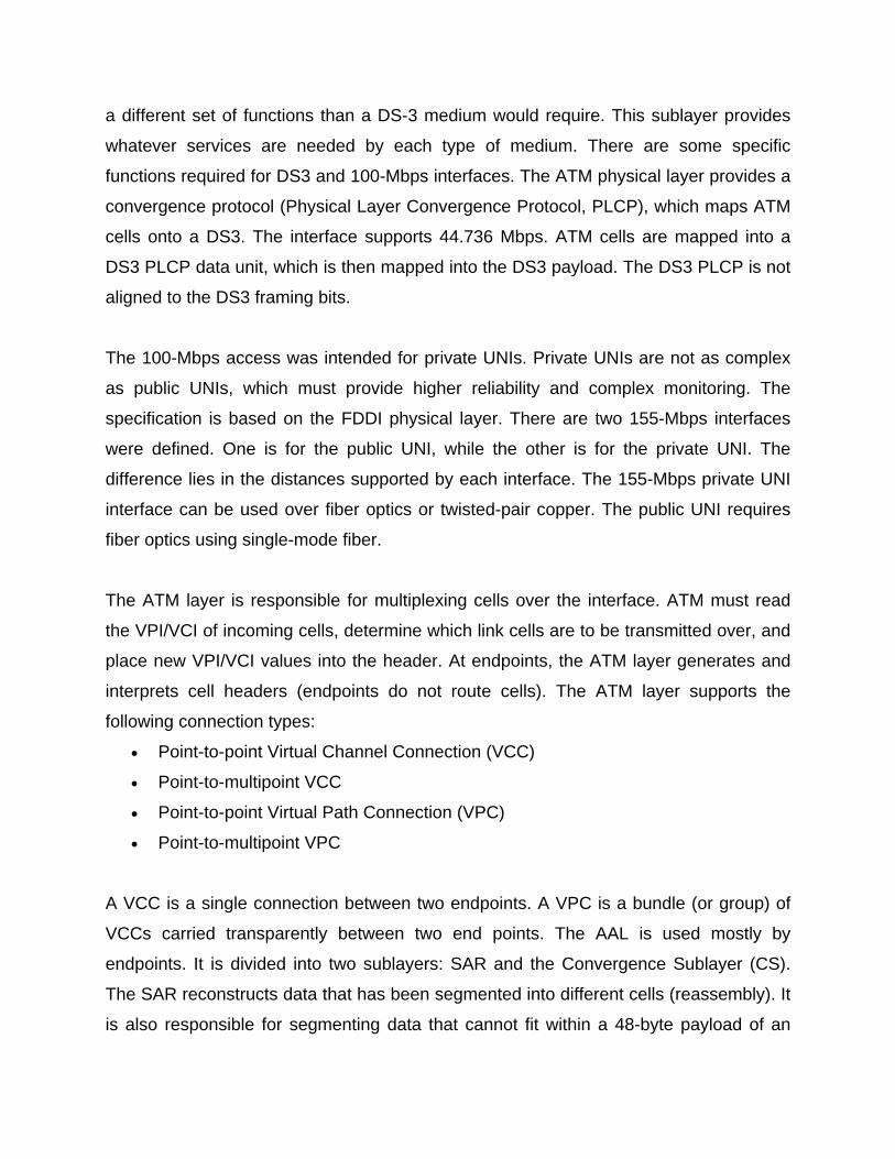
a different set of functions than a DS-3 medium would require. This sublayer provides

whatever services are needed by each type of medium. There are some specific

functions required for DS3 and 100-Mbps interfaces. The ATM physical layer provides a

convergence protocol (Physical Layer Convergence Protocol, PLCP), which maps ATM

cells onto a DS3. The interface supports 44.736 Mbps. ATM cells are mapped into a

DS3 PLCP data unit, which is then mapped into the DS3 payload. The DS3 PLCP is not

aligned to the DS3 framing bits.

The 100-Mbps access was intended for private UNIs. Private UNIs are not as complex

as public UNIs, which must provide higher reliability and complex monitoring. The

specification is based on the FDDI physical layer. There are two 155-Mbps interfaces

were defined. One is for the public UNI, while the other is for the private UNI. The

difference lies in the distances supported by each interface. The 155-Mbps private UNI

interface can be used over fiber optics or twisted-pair copper. The public UNI requires

fiber optics using single-mode fiber.

The ATM layer is responsible for multiplexing cells over the interface. ATM must read

the VPI/VCI of incoming cells, determine which link cells are to be transmitted over, and

place new VPI/VCI values into the header. At endpoints, the ATM layer generates and

interprets cell headers (endpoints do not route cells). The ATM layer supports the

following connection types:

• Point-to-point Virtual Channel Connection (VCC)

• Point-to-multipoint VCC

• Point-to-point Virtual Path Connection (VPC)

• Point-to-multipoint VPC

A VCC is a single connection between two endpoints. A VPC is a bundle (or group) of

VCCs carried transparently between two end points. The AAL is used mostly by

endpoints. It is divided into two sublayers: SAR and the Convergence Sublayer (CS).

The SAR reconstructs data that has been segmented into different cells (reassembly). It

is also responsible for segmenting data that cannot fit within a 48-byte payload of an

ATM cell (segmentation). The CS determines the class of service to be used for a

transmission. This will depend on the bit rate (constant or variable bit rate), the type of

data, and the type of service to be provided (connection-oriented or connectionless).

The quality of service parameters necessary for the transmission are determined by the

class of service assigned

8.2.2 ATM Overview - ATM Header and Payload

The ATM cell is 53 bytes in length. The first 5 bytes are used for the header. The

payload portion of the cell is 48 bytes. Keep in mind as we discuss the protocol that the

payload is also used for the AAL overhead and any other overhead from upper layers.

There are two formats for the ATM header as shown in figure 8.8. One header is used

for the UNI, while the other is used for the NNI. The difference lies in the Generic Flow

Control (GFC) parameter found in the UNI header. The GFC is not supported in the

public network, nor was it intended to be.

The header is placed in front of the payload (it arrives first). There is no trailer used in

ATM. Figure shows the two-header formats. In the UNI header, the GFC can be used to

throttle traffic from a specific destination. The GFC values are not currently defined, but

the intent is that the GFC could be used to provide flow control from the user to the

network (and vice versa). This parameter is not used out in the public network and is

overwritten by network nodes.

Figure 8.8: ATM Header (UNI & NNI)

Two modes are defined for GFC, controlled and uncontrolled. Controlled GFC allows

subscriber equipment to control flow of ATM cells, however, the values for this have not

been defined. They are of local significance only, which means they are related to a link

connection at a switch and used to communicate with the remote end of a link.

Uncontrolled GFC simply means that GFC is not supported, and the parameter is set to

all zeroes. The VPI is used to identify a group of virtual channels within the same

endpoint. This is the form of addressing supported in ATM. Rather than identifying

millions of unique nodes, ATM addressing identifies a connection. A virtual channel is

used for a communication link. Each virtual channel is identified by the VCI.

The meta signaling channel is a dedicated channel used to establish virtual channel

connections between two endpoints. The virtual paths are predetermined at the time of

installation (either through administration or by the service provider). Virtual paths can

be negotiated by the user or the network using meta signaling. This means the

establishment or release of virtual paths can be controlled by the user or the network.

Following the VPI and the VCI is the Payload Type Indicator (PTI). This parameter

indicates the type of data found in the payload portion of the cell. Remember that the

payload is not always data. There could be signaling information, network management

messages, and other forms of data. These are identified by the PTI. The PTI is followed

by the Cell Loss Priority (CLP) parameter. This is used to prioritize cells. In the event of

congestion or some other trouble, a node can discard cells that have a CLP value of 1

(considered low priority). If the CLP value is 0, the cell has a high priority and should

only be discarded if it cannot be delivered.

The last byte in the header is the Header Error Control (HEC) parameter, which is used

for error checking and cell delineation. Only the header is checked for errors. The HEC

works like other error checking methods, where an algorithm is run on the header and

the value placed in the HEC. ATM is capable of fixing single bit errors but not multiple

bit errors. An ATM node places itself in error correction mode during normal operation.

If a single bit error is detected in the header, the data in the header is small enough that

the error correctio algorithm can determine which bit is in error and correct it. If a multibit

error is detected, the node places itself in error detection mode. Errors are not corrected

while in this mode. The node remains in error detection mode as long as cells are

received in error. When cells are received without error, the node places itself back into

error correction mode.

8.3 Summary The ISDN is intended to be a worldwide public telecommunications network to replace

existing public telecommunications networks and deliver a wide variety of services. The

ISDN is defined by the standardization of user interfaces and is implemented as a set of

digital switches and paths supporting a broad range of traffic types and providing value-

added processing services. ATM is a packet switching protocol. It encodes the data into

small fixed size cells. The ATM cell is 53 bytes in length. The first 5 bytes are used for

the header. The payload portion of the cell is 48 bytes. ATM was originally designed to

operate over fiber optics but because of the slow deployment of fiber, was later modified

to operate over copper and coaxial facilities as well.

8.4 Self Assessment Questions

1. Define ISDN and explain its principle.

2. Explain different ISDN connections with the help of suitable diagram.

3. Name and explain the functions of three types of channels.

4. Explain ISDN Protocol Architecture.

5. What is the full form of ATM? Show the different layers of ATM.

6. Write short note on ATM Header.

8.5 References / Suggested Readings

• Computer Networks (3rd & 4th Edition), Andrew S. Tannenbaum, PHI /

Pearson’s Publications

• Computer Networks (2nd edition), Uyless Black, PHI Publication

• Computer Network, ED Tittle, Tata MacGraw Hills Publications