11

Ch3: Productivity, Output, and Employment

Abel & Bernake: Macro Ch3

Varian: Ch10, Ch19

22

Chapter Outline

The Production Function The Demand for Labor The Supply of Labor Labor Market Equilibrium Unemployment Relating Output and Unemployment: Okun’s Law

33

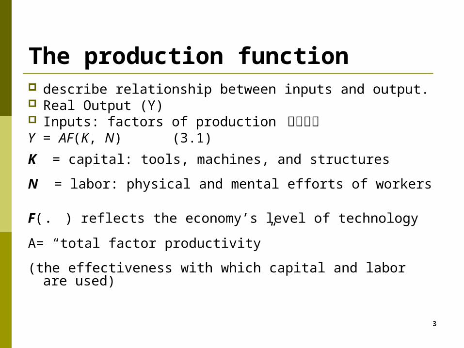
The production function describe relationship between inputs and output. Real Output (Y) Inputs: factors of production 生產要素Y = AF(K, N) (3.1)

K = capital: tools, machines, and structures

N = labor: physical and mental efforts of workers

F( ． ) reflects the economy’s level of technology

A= “total factor productivity”

(the effectiveness with which capital and labor are used)

44

Table 3.1 The Production Function of the United States, 1979-2007

Assumes constant returns to scale Cobb-Douglas production function works well for U.S. economy:Y = A K0.3 N0.7 (3.2)

Productivity grew slowly in 1980s and the first half of the 1990s, but increased since the mid-1990s.

55

Returns to scale: Initially Y1 = AF (K1 , N1 )

Scale all inputs by the same factor z:

K2 = zK1 and N2 = zN1

(e.g., if z = 1.25, then all inputs are increased by 25%)

What happens to output, Y2 = F (K2, N2 )?

If constant returns to scale, Y2 = zY1

If increasing returns to scale, Y2 > zY1

If decreasing returns to scale, Y2 < zY1

66

Examples

2 2

2

F K N K N CRS

F K N K N IRS

F K N KN CRS

F K N K N DRS

KF K N CRS

N

( , ) :

( , ) :

( , ) :

( , ) :

( , ) :

7

Diminishing marginal returns: diminishing MPN

Marginal Product of Labor:

Diminishing marginal returns: diminishing MPN

Suppose N while holding K fixed fewer machines per worker lower worker productivity

Marginal Product of Capital:

N

Y YMP

N N

K

Y YMP

K K

88

Fig 3.1 The Production Function Relating Output and Capital Fig 3.2 The marginal product of capital

K

Y YMP

K K

99

Youtput

Fig 3.3: MPN ( K fixed ) Diminishing marginal returns

Nlabor

( , )Y AF K L

1

MPN

1

MPN

1MPN

As more labor is added, MPN

Slope of the production function equals MPN

),( NKAFN

Y

N

YMP NN

N

1010

Eg, diminishing MPN Which of these production functions have

diminishing marginal returns to labor?

F K N K Na) 2 15( , )

b) ( , )F K N KN

( , )F K N K Nc) 2 15

1111

Supply shocks

Supply shock = productivity shock = a shift in an economy’s production function (Fig. 3.4)

Supply shocks affect the amount of output that can be produced for a given amount of inputs

Negative (adverse) shock: Usually slope of production function decreases at each level of input (eg, if shock causes parameter A to decline)

Positive shock: Usually slope of production function increases at each level of output (eg, if parameter A increases)

eg, weather, inventions and innovations, government regulations, oil prices

1212

Fig3.4 An adverse supply shock that lowers the MPN

1313

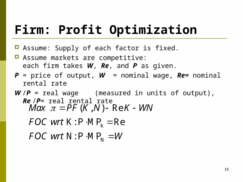
Firm: Profit Optimization Assume: Supply of each factor is fixed. Assume markets are competitive:

each firm takes W, Re, and P as given.

P = price of output, W = nominal wage, Re= nominal rental rate

W /P = real wage (measured in units of output), Re /P= real rental rate

k

N

( , ) Re

K: P MP Re

N: P MP

Max PF K N K WN

FOC wrt

FOC wrt W

1414

Demand for labor

benefit = MPN, cost = real wage

A firm hires each unit of labor if the cost does not exceed the benefit.

MCFOCimizationProfit Max

wP

WW

?P :Y) (

MP ,MPP NN

laborfor Demand :MP

MP

N

N

P

WP

W

1515

Fig 3.5: MPN = Demand for labor

Each firm hires labor up to the point where MPN = W/P.

Each firm hires labor up to the point where MPN = W/P.

Units of output

Units of labor, N

MPN, Labor demand

Real wage

Quantity of labor demanded

1616

Summary 2

1717

Labor Market: the equilibrium real wageUnits of output

Units of labor, N

MPN, Labor demand

equilibrium real wage

Labor supply

LN

1818

A↑ or K↑→ ? → ?Fig 3.6 The effect of a beneficial supply shock on

labor demand (here A↑)

1919

Summary 3

2020

The Supply of Labor

Aggregate supply of labor is the horizontal sum of individuals’ labor supply

Labor supply of individuals depends on consumption-leisure choice

2121

Individual: Utility Optimization The consumption-leisure trade-off

Max U(C, L)St. time constraint: L + h = T budget constraint: C ≦ wh + VU: utility, C: consumption, L: leisure, h: working hours, T: time endowment,

w: real wage rate, V: nonlabor income, w: price of leisure, opportunity cost of leisure Constraint combined: C ≦ w(T-L) + V Trade-off: more h, less L, but more income and more C

22

Optimal consumption and leisure ( 參考 )h > 0: working, h=0: not in the LFat point E: corner solution -- indifferent

$1100

$1200A Y

$500 P

U1

$100U0

U*

E

110

110

40

70

0

0

Hours of Work

Hours of Leisure

Consumption ($)

2323

A pure income effect (IE): V↑

Winning a lottery : V↑ A pure income effect:

Demand for normal goods increase: C↑, L↑ Winning the lottery: no SE

because it doesn’t affect the reward for working

L↑=> h↓

2424

An increase in real wages: w↑

An increase in the real wage : w↑ Substitution effect (SE):

w↑: price of leisure ↑

Use cheaper C to substitute more costly L

=> C↑,L↓ => h↑ Income effect (IE):

w↑for same h => income ↑ => C↑,L ↑ => h ↓ w↑total effect: has offsetting IE and SE h ↑ if SE > IE

h ↓ if SE < IE

2525

Fig 3.7 labor supply curve of an individual worker

26

Temporary vs. Permanent increase in wOptimization over time (Ch4)

ISE: intertemporal substitution effect ISE between current C and future C’

ISE between current L and future L’ If temporary w↑: strong ISE + weak IE

ISE > IE => L↓, h ↑ If permanent w↑ : weak ISE + strong IE

ISE < IE => L ↑, h ↓ Empirical evidence support the implication.

2727

Aggregate labor supply

When current real wage risesSome people work more hoursOther people enter labor force

Result: Aggregate labor supply curve slopes upward

2828

Fig 3.8 The effect on labor supply of an increase in wealth

2929

Factors that shifts aggregate labor supply

Factors increasing labor supplyDecrease in wealthDecrease in expected future real wageIncrease in working-age population

(higher birth rate, immigration)Increase in labor force participation

(increased female labor participation, elimination of mandatory retirement)

3030

Summary 4

3131

Application:comparing U.S. and European labor markets

Unemployment rates were similar in the U.S. and Europe in 1970s and 1980s,

but are higher in Europe since then (Fig. 3.9) 3 reasons for higher unemployment rates in Europe:

generous unemployment insurance systems,

high tax rates,

government policies that interfere with labor markets

3232

Fig 3.9 Unemployment rates in the U.S. and Europe, 1982-2008

Source: OECD Factbook 2009, Harmonised Unemployment Rates.

3333

Labor Market Equilibrium

Equilibrium: Labor supply equals labor demand Classical model of the labor market:

real wage adjusts quickly Determines full-employment level of employment

and market-clearing real wage Problem with classical model:

can’t study unemployment

3434

Fig 3.10 Labor market equilibrium

3535

Full-employment output

Full-employment output = potential output = level of output when labor market in equilibrium

Yf= AF(K, Nf) (3.4)

An adverse supply shock: A↓

MPN =AFN ↓→ DN↓→ Nf↓ (Fig. 3.11)

Yf ↓ because both A↓and Nf ↓

),( NKAFY

3636

Fig 3.11 Effects of a temporary adverse supply shock on the labor market

Sources: Producer price index for fuels and related products and power from research.stlouisfed.org/fred2/series/PPIENG; GDP deflator from research.stlouisfed.org/fred2/GDPDEF. Data were scaled so that the relative price of energy equals 100 in year 2000.

3737

Application: output, employment, and the real wage during oil price shocks

Sharp oil price increases in 1973–1974, 1979–1980, 2003–2008 (Fig. 3.12) Adverse supply shock—lowers labor demand,

employment, the real wage, and the full-employment level of output

First two cases: U.S. economy entered recessions Research result: 10% increase in price of oil

reduces GDP by 0.4 percentage points

3838

Fig 3.12 Relative price of energy,1960-2008

3939

Determination of factor prices （補充）Varian: 19.7-19.9 and Appendix

Factor prices are determined by supply and demand in factor markets.

Assume: Supply of each factor is fixed. Assume markets are competitive:

each firm takes W, Re, and P as given.

( , ) Re

K : Re

N :K

N

Max PF K N K WN

FOC wrt P MP

FOC wrt P MP W

40

Why assuming CRS?Eg, Cobb-Douglas Production Function

A is exogenous, CRS: α+β=1 β=1-α

Each factor’s MP is proportional to its AP.

K

N

YMP AK N

KY

MP AK NN

1 1

(1 ) (1 )

Y AK N AK N1

41

Neoclassical Theory of Distribution: C-D production function in competitive markets

In the competitive market: C-D production function (CRS) constant factor shares:

capital income≡ labor income ≡

= capital’s share of total income1- = labor’s share of total income

Assumes CRS Cobb-Douglas production function works well for U.S. economy: Y = A K0.3 N0.7 (3.2)

Re( ) KP K MP K Y

( ) (1 )WNP N MP N Y

Re( ) , ( )WK NP PMP MP

42

The ratio of labor income to total income in the U.S.

0

0.2

0.4

0.6

0.8

1

1960 1970 1980 1990 2000

Labor’s share of total income

Labor’s share of income is approximately constant over time.

(Hence, capital’s share is, too.)

Labor’s share of income is approximately constant over time.

(Hence, capital’s share is, too.)

43

Taiwan data: labor share (%)薪資報酬佔所得比例

0

20

40

60

80

100

1997 1998 1999 2000 2001 2002 2003 2004 2005 2006

年度

%

薪資報酬佔所得比例

44

Neoclassical Theory of Distribution

Proof that

Exhaustion of the product imply zero profits for competitive

firms in the LR. Since π=0 for all periods,

can ignore intertemporal analysis:

profit maximization over-time

Re( ) ( )WN K P PMP N MP N K Y

45

Ch3: 勞動力之分類

臺灣地區總人口

未滿十五歲人口 十五歲以上人口

監管人口 武裝勞動力 （現役軍人）

民間人口

（民間）勞動力 非勞動力

就業者 失業者

4646

Fig 3.13 Worker flow:Changes in employment status in a typical month (June 2007)

4747

Duration of Unemployment 失業期間

Duration of unemployment

（ length of unemployment spell ） Most unemployment spells are of short duration Most unemployed people on a given date are

experiencing unemployment spells of long duration

4848

3 types of unemployment

Frictional unemployment 摩擦性失業Search activity of firms and workers due to heterogeneity.

Matching process takes time.

Structural unemployment 結構性失業Reallocation of workers (lack of new skill) out of shrinking industries or depressed regions:

matching takes a long time

Cyclical unemployment 景氣性失業

4949

The natural rate of unemployment

The natural rate of unemployment ( )

when output and employment are at full-employment levels

= frictional + structural unemployment Cyclical unemployment:

difference between actual unemployment rate and natural rate of unemployment,

u

uu

u

5050

Okun’s Law:Relating Output and Unemployment Relationship between

output (relative to full-employment output) and cyclical unemployment

(3.5)

Alternative formulation:

if average growth rate of full-employment output is 3%:

Y/Y = 3 – 2 u (3.6)

2( )Y Y

u uY

5151

Fig 3.14 Okun’s Law in the US: 1951-2008

Sources: Real GDP growth rate from Table 1.1.1 from Bureau of Economic Analysis Web site, www.bea.gov/bea/dn/nipaweb. Civilian unemployment rate for all civilian workers from Bureau of Labor Statistics Web site, data.bls.gov.

52

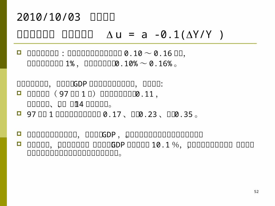
2010/10/03 工商時報台灣歐肯係數 四小龍最小 u = a -0.1(Y/Y ) 主計處研究報告 : 現階段我國的歐肯係數約在 0.10 ～ 0.16 之間，

即經濟成長每提升 1% ，只能降低失業率 0.10% ～ 0.16% 。

亞洲四小龍最小，顯示台灣 GDP 成長對改善失業的效果，相對較低 : 金融海嘯前（ 97 年第 1 季）台灣的歐肯係數為 0.11 ，

係數低於美、德、英等 14 個先進國家。 97 年第 1 季新加坡的歐肯係數為 0.17 、香港 0.23 、南韓 0.35 。

台灣致力發展高科技產業，雖能創造 GDP ，但由於所能提供的就業機會非常有限。

主計處表示，金融海嘯期間，台灣的實質 GDP 衰退幅度達 10.1 ％，台灣的歐肯係數較低，卻也使得台灣在金融海嘯期間失業率上升幅度相對較小。