1

Ch4: Consumption, Saving, and Investment

Abel & Bernake: Macro Ch3

Mankiw: Macro Ch3

2

Chapter Outline

Appendix: micro-foundation of Macro Consumption and Saving Investment Goods Market Equilibrium

3

Aggregate Demand:Demand for goods & services

Assume a closed economy: NX=0, NFP=0

Components of aggregate demand:

AD = Cd+Id+G+NX = Cd+Id+G Desired consumption (Cd) Desired investment (Id)

4

Consumption C Traditional: Keynesian setup

Disposable income

total income minus total taxes:

Yd ≡ Y – T.

Consumption function: C = C(Yd) = a+bYdassume Yd C

Marginal propensity to consume (MPC)

d

CMPC

Y

5

Appendix: Intertemporal analysis utility maximization over-time With micro-foundation:

Cd = optimal C*

= C (lifetime wealth, real interest rate)

= C (current income, future income, real interest rate)

Desired consumption and saving: function of r

Sd = Y – Cd – G (4.1)

6

Saving is for future consumption

Trade-off between current consumption and future consumption

The price of 1 unit of current consumption is (1 + r) units of future consumption, where r is the real interest rate

Consumption-smoothing motive: the desire to have a relatively even pattern of consumption over time

7

Consumption and Saving

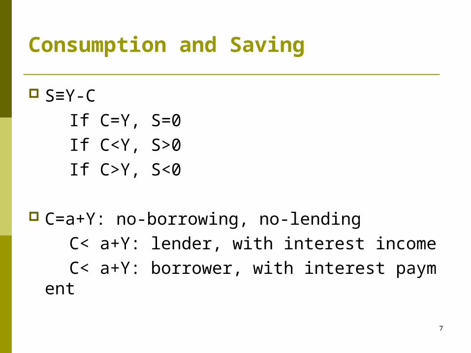
S≡Y-C

If C=Y, S=0

If C<Y, S>0

If C>Y, S<0

C=a+Y: no-borrowing, no-lending

C< a+Y: lender, with interest income

C< a+Y: borrower, with interest payment

8

Effect of changes in current income

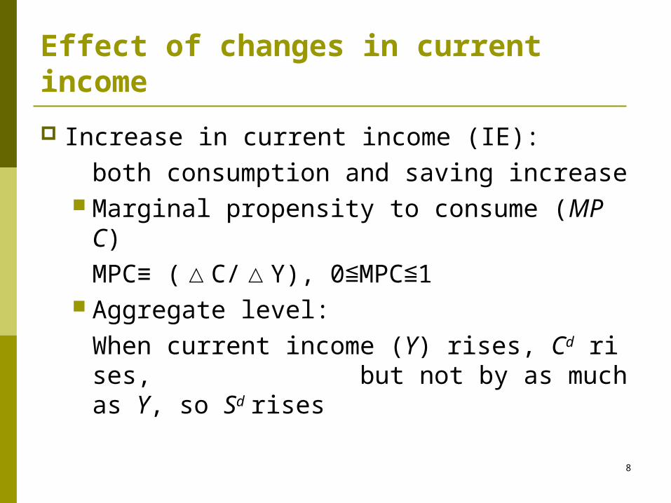
Increase in current income (IE):

both consumption and saving increase Marginal propensity to consume (MPC)

MPC≡ (△C/△Y), 0 MPC 1≦ ≦ Aggregate level:

When current income (Y) rises, Cd rises, but not by as much as Y, so Sd rises

9

Effect of changes in expected future income

Higher expected future income leads to more consumption today, so saving falls.

10

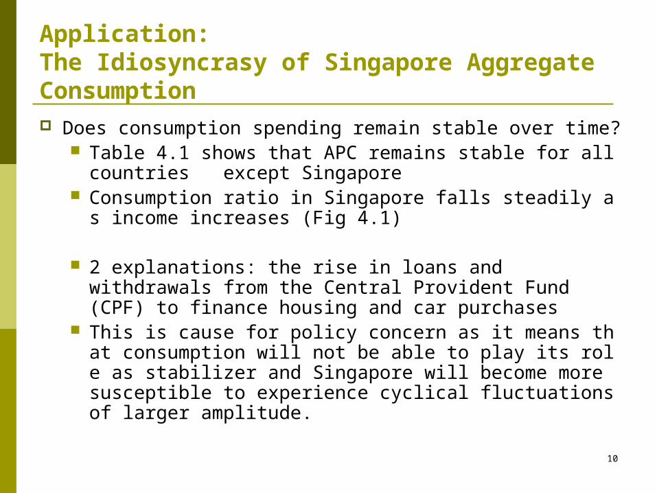
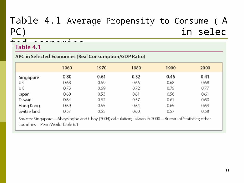
Application: The Idiosyncrasy of Singapore Aggregate Consumption

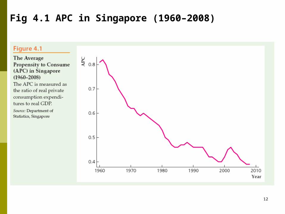
Does consumption spending remain stable over time? Table 4.1 shows that APC remains stable for all countries excep

t Singapore Consumption ratio in Singapore falls steadily as income increase

s (Fig 4.1)

2 explanations: the rise in loans and withdrawals from the Central Provident Fund (CPF) to finance housing and car purchases

This is cause for policy concern as it means that consumption will not be able to play its role as stabilizer and Singapore will become more susceptible to experience cyclical fluctuations of larger amplitude.

11

Table 4.1 Average Propensity to Consume ( APC) in selected economies

12

Fig 4.1 APC in Singapore (1960–2008)

13

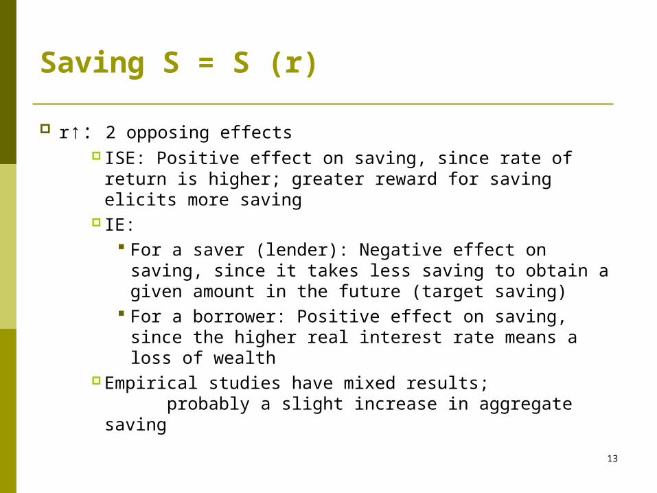
Saving S = S (r)

r↑: 2 opposing effects ISE: Positive effect on saving, since rate of return is

higher; greater reward for saving elicits more saving IE:

For a saver (lender): Negative effect on saving, since it takes less saving to obtain a given amount in the future (target saving)

For a borrower: Positive effect on saving, since the higher real interest rate means a loss of wealth

Empirical studies have mixed results; probably a slight increase in aggregate saving

14

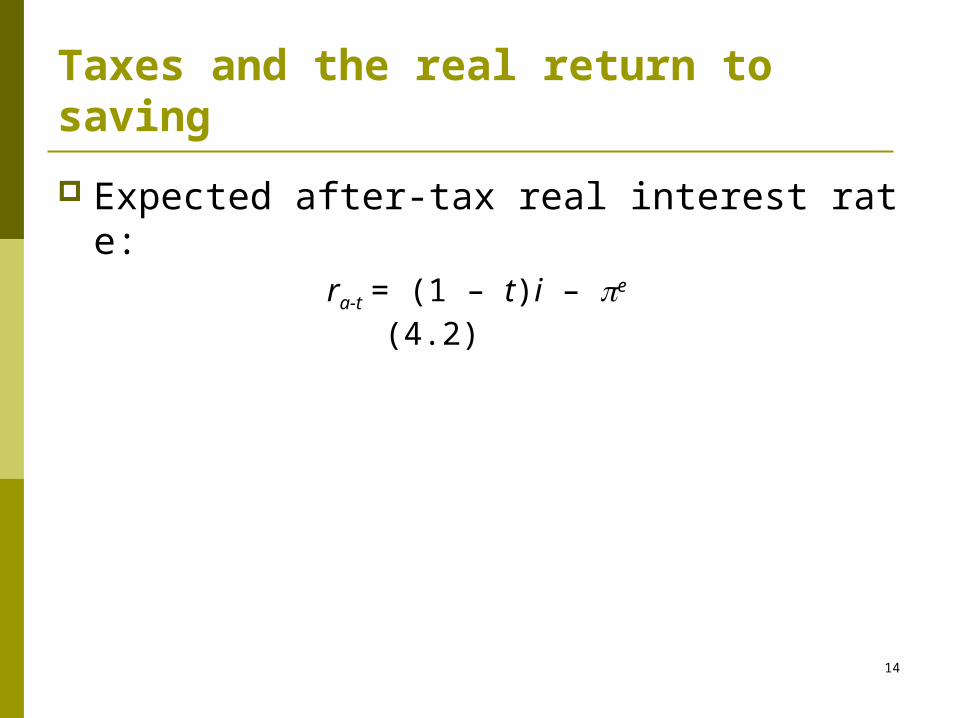
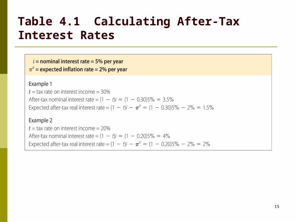
Taxes and the real return to saving

Expected after-tax real interest rate:ra-t = (1 – t)i – e

(4.2)

15

Table 4.1 Calculating After-Tax Interest Rates

16

In touch with data and research: interest rates

different interest rates, default risk, term structure (yield curve), and tax status Since interest rates often move together, we frequently refe

r to “the” interest rate Yield curve:

relationship between life of a bond and interest rate

殖利率曲線 : 零息債券的殖利率與其到期日的關係橫軸為各到期期限 (time to maturity) ，縱軸為相對應之到期殖利率 (yield to maturity) ，用以描述兩者之關係。

17

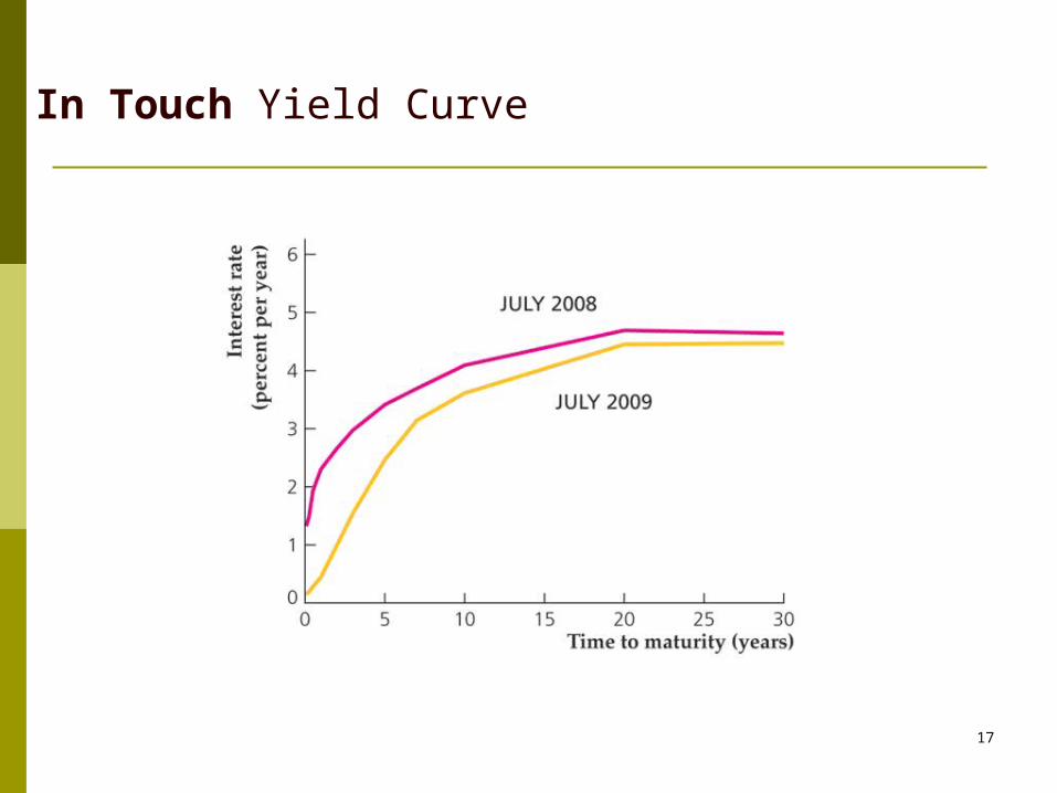
In Touch Yield Curve

18

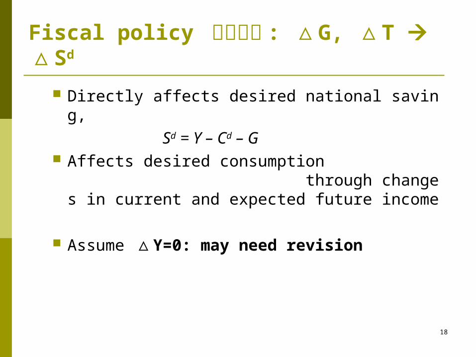
Fiscal policy 財政政策 : △G, △T △Sd

Directly affects desired national saving,

Sd = Y – Cd – G Affects desired consumption throug

h changes in current and expected future income

Assume Y=0: may need revision△

19

Fiscal policy:

Government purchases (temporary G↑)

Higher G financed by higher current taxes reduces after-tax income, lowering desired consumption

Even true if financed by higher future taxes, if people realize how future incomes are affected

Since Cd declines less than G rises, national saving (Sd = Y – Cd – G) declines

So government purchases reduce both desired consumption and desired national saving.

20

Fiscal policy: Tax cut (T↓, G=0)△Ricardian equivalence proposition (Appendix)

Lump-sum tax cut today,

??

If tax change affects only the timing of taxes, not their ultimate amount (present value)

no change in consumption

(Ricardian equivalence proposition) ???

21

Ricardian equivalence proposition

In practice, people may not see that future taxes will rise if taxes are cut today; then a tax cut leads to increased desired consumption and reduced desired national saving.

22

Application: How consumers respond to tax rebates

The government provided a tax rebate in 2008, hoping to stimulate the economy.2008 年 5 月美國國稅局 (IRS) 會有特別退稅 （個人 300-600 元， 17 歲以下小孩每位 300 元 ) ：美國振興經濟 (Economic Stimulus Act of 2008) 法案的一部分

Research by Shapiro and Slemrod suggests that consumers did not increase spending much in 2001, when the government provided a similar tax rebate.

23

Application: How consumers respond to tax rebates

New research by Agarwal, Liu, and Souleles have different findings from their study on credit-card payments, purchases, and debt over time.

People getting the tax rebates initially made additional payments on their credit cards, paying down their balances; but after nine months they had increased their purchases and had more credit-card debt than before the tax rebate.

Younger people, who were more likely to face binding borrowing constraints, increased their purchases on credit cards the most of any group in response to the tax rebate.

People with high credit limits also spent less, behaved more in the manner suggested by Ricardian equivalence.

24

Summary 5

25

Investment Investment plays a crucial role in economic growth. Investment fluctuates sharply over the business cycle,

so we need to understand investment to understand the business cycle.

26

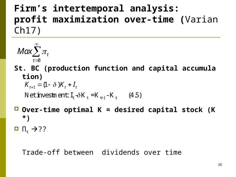
Firm’s intertemporal analysis: profit maximization over-time (Varian Ch17)

St. BC (production function and capital accumulation)

Over-time optimal K = desired capital stock (K*)

Πt ??

Trade-off between dividends over time

0t

t

Max

1

t t t+1 t

(1 )

Net investment: I - K =K - K (4.5)t t tK K I

27

Desired capital stock (K*)

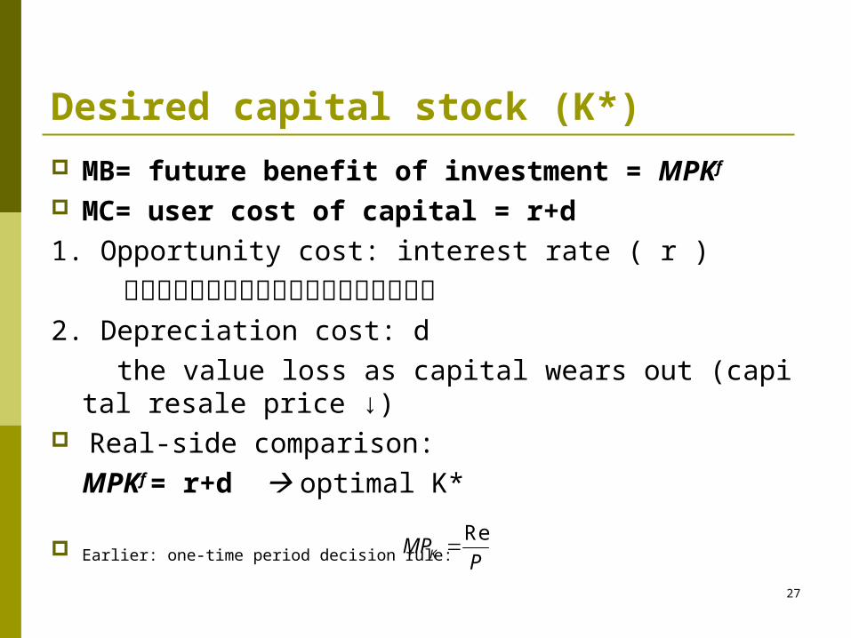
MB= future benefit of investment = MPKf MC= user cost of capital = r+d

1. Opportunity cost: interest rate ( r )

股利原可存銀行賺利息或借錢融資需繳利息2. Depreciation cost: d

the value loss as capital wears out (capital resale price ↓) Real-side comparison:

MPKf = r+d optimal K*

Earlier: one-time period decision rule: ReKMP

P

28

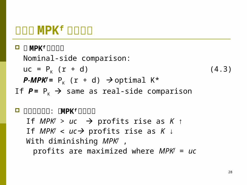
課本將 MPKf 視為名目 若 MPKf 視為實質

Nominal-side comparison:

uc = PK (r + d) (4.3)

P MPK‧ f = PK (r + d) optimal K*

If P = PK same as real-side comparison

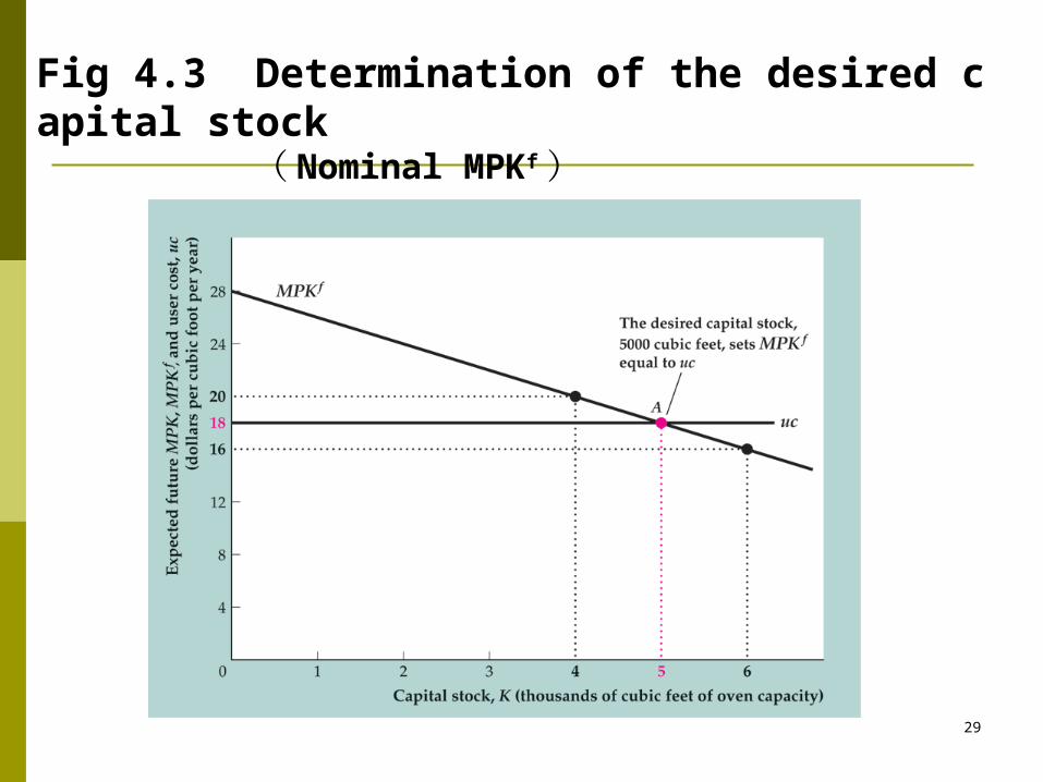
以下採用課本：將 MPKf 視為名目If MPKf > uc profits rise as K ↑ If MPKf uc profits rise as K ↓With diminishing MPKf ,

profits are maximized where MPKf = uc

29

Fig 4.3 Determination of the desired capital stock （ Nominal MPKf ）

30

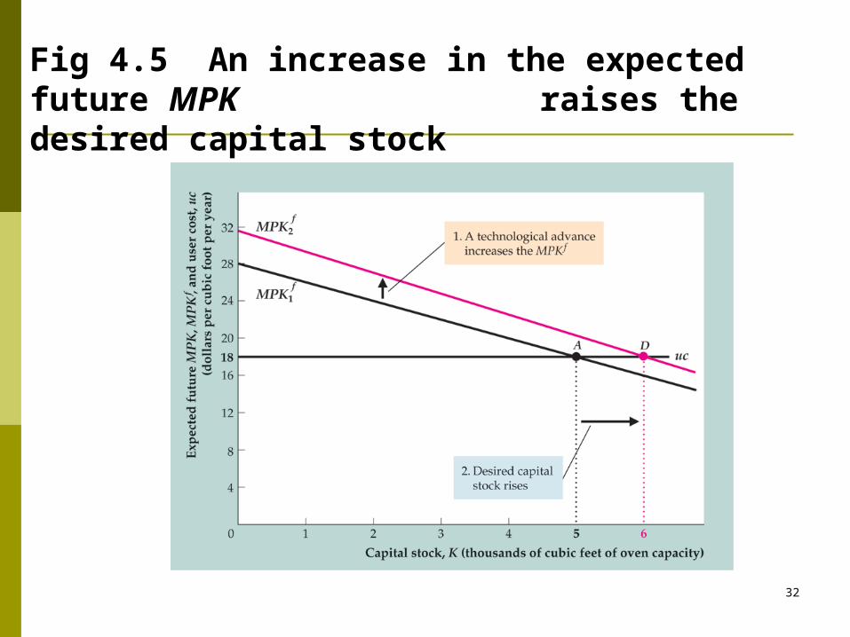
Changes in the desired capital stock ( K*)△

△r, d, △ △PK uc△ Technological changes △MPKf

Factors that change user cost of capital (Fig. 4.4) Or factors that shift the MPKf curve (Fig. 4.5)the desired capital stock to change

31

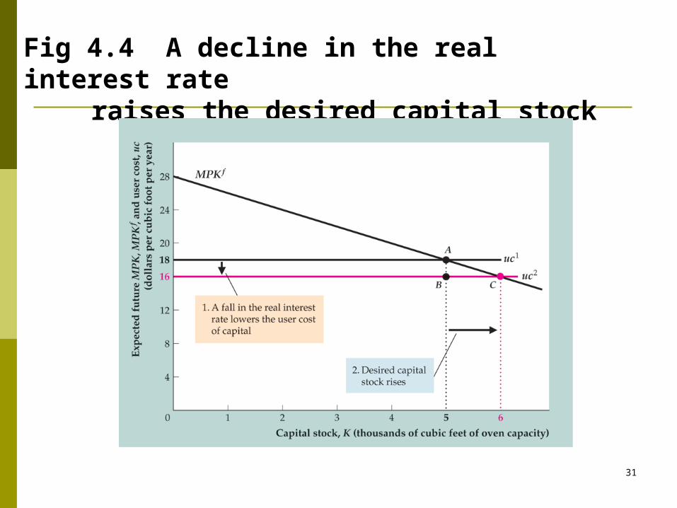
Fig 4.4 A decline in the real interest rate raises the desired capital stock

32

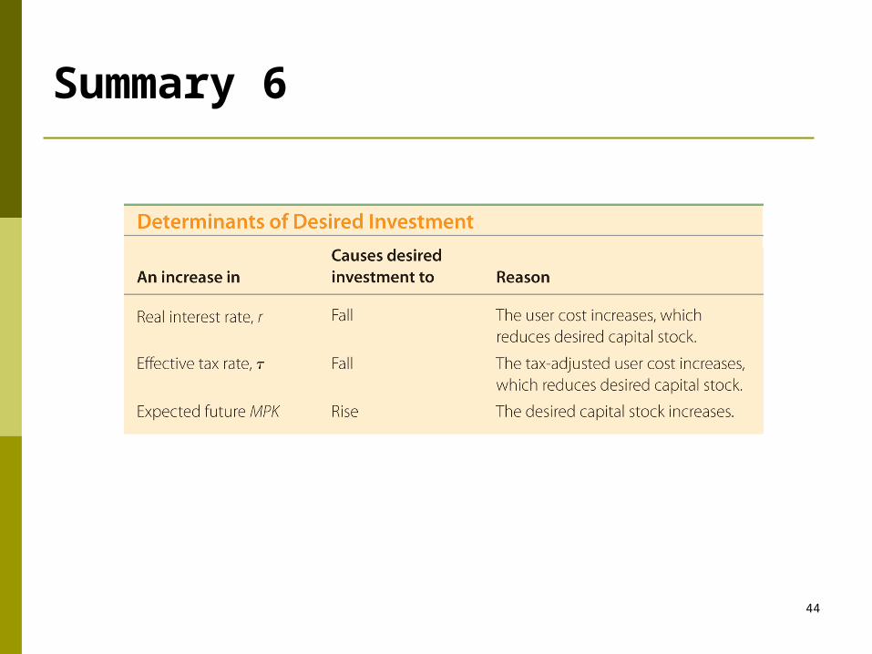
Fig 4.5 An increase in the expected future MPK raises the desired capital stock

33

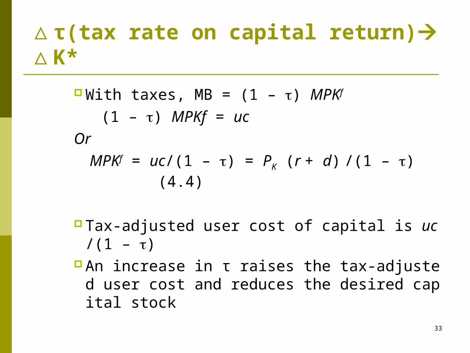
△τ(tax rate on capital return) K*△

With taxes, MB = (1 – ) MPKf

(1 – ) MPKf = uc

Or

MPKf = uc/(1 – ) = PK (r + d) /(1 – ) (4.4)

Tax-adjusted user cost of capital is uc/(1 – ) An increase in τ raises the tax-adjusted user cost and red

uces the desired capital stock

34

the effective tax rate

In reality, there are complications to the tax-adjusted user cost We assumed that firm revenues were taxed

In reality, profits, not revenues, are taxed So depreciation allowances reduce the tax paid by firms,

because they reduce profits Investment tax credits reduce taxes when firms make new

investments Summary measure: the effective tax rate—the tax rate on firm

revenue that would have the same effect on the desired capital stock as do the actual provisions of the tax code

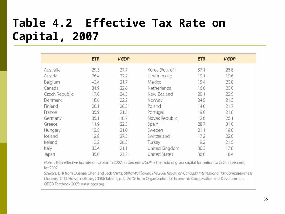
Table 4.2 shows effective tax rates for many different countries

35

Table 4.2 Effective Tax Rate on Capital, 2007

36

Application: measuring the effects of taxes on investment

Do changes in the tax rate have a significant effect on investment?

A 1994 study by Cummins, Hubbard, and Hassett found that after major tax reforms, investment responded strongly; elasticity about –0.66 (of investment to user cost of capital)

37

From the desired capital stock to investment

Gross investment It = Kt+1 – Kt + dKt

If firms can change their capital stocks in one period, then Kt+1 = K* (the desired capital stock)

It = K* – Kt + dKt (4.6)

Investment has two parts Desired net increase in the capital stock over the year (K

* – Kt)

Investment needed to replace worn-out capital (dKt)

With adjustment costs lags

? -- partial adjustment

38

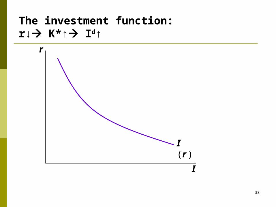
The investment function:r↓ K*↑ Id↑

r

I

I

(r )

39

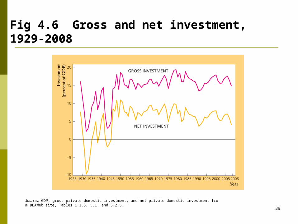
Fig 4.6 Gross and net investment, 1929-2008

Sources: GDP, gross private domestic investment, and net private domestic investment from BEAWeb site, Tables 1.1.5, 5.1, and 5.2.5.

40

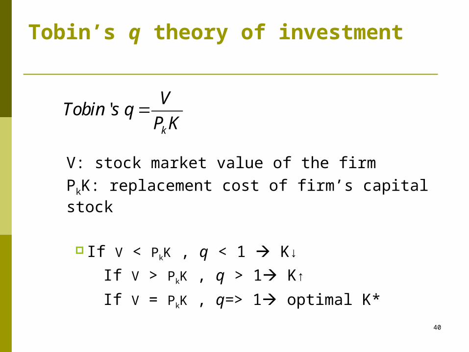
Tobin’s q theory of investment

V: stock market value of the firm

PkK: replacement cost of firm’s capital stock

If V < PkK , q < 1 K↓

If V > PkK , q > 1 K↑

If V = PkK , q=> 1 optimal K*

' k

VTobin s q

P K

41

Tobin’s q theory of investment

Firms change investment

in the same direction as the stock market.

If r↓? , q > 1 K↑ If Pk↓ ? q > 1 K↑ MPKf ↑ V ↑ q > 1 K↑

Data show general tendency of investment to rise when stock market rises; but relationship isn’t strong because many other things change at the same time (Figure 4.7)

42

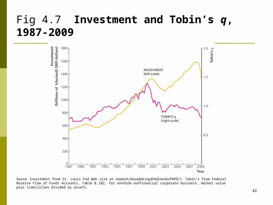
Fig 4.7 Investment and Tobin’s q, 1987-2009

Source: Investment from St. Louis Fed Web site at research.stlouisfed.org/fred2/series/PNFIC1; Tobin’s from FederalReserve Flow of Funds Accounts, Table B.102, for nonfarm nonfinancial corporate business, market value plus liabilities divided by assets.

43

Investment in inventories and housing

Marginal product of capital and user cost also apply, as with equipment and structures

44

Summary 6

45

Government spending, G G = govt spending on goods and services. G excludes transfer payments

(e.g., social security benefits, unemployment insurance benefits).

Assume government spending and total taxes are exogenous:

and G G T T

46

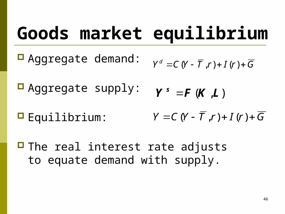
Goods market equilibrium Aggregate demand:

Aggregate supply:

Equilibrium:

The real interest rate adjusts to equate demand with supply.

GrIrTYCY d )(),(

( , )sY F K L

GrIrTYCY )(),(

47

Goods Market Equilibrium

The real interest rate adjusts to bring the goods market into equilibrium Y = Cd + Id + G (4.7)

goods market equilibrium condition Differs from income-expenditure identity, a

s goods market equilibrium condition need not hold; undesired goods may be produced, so goods market won’t be in equilibrium.

48

Goods Market Equilibrium

Alternative representation for a closed economy:

Y= Cd + Id + G

Sd = Y – Cd – G,

Sd = Id (4.8)

saving-investment diagram (Fig. 4.8)

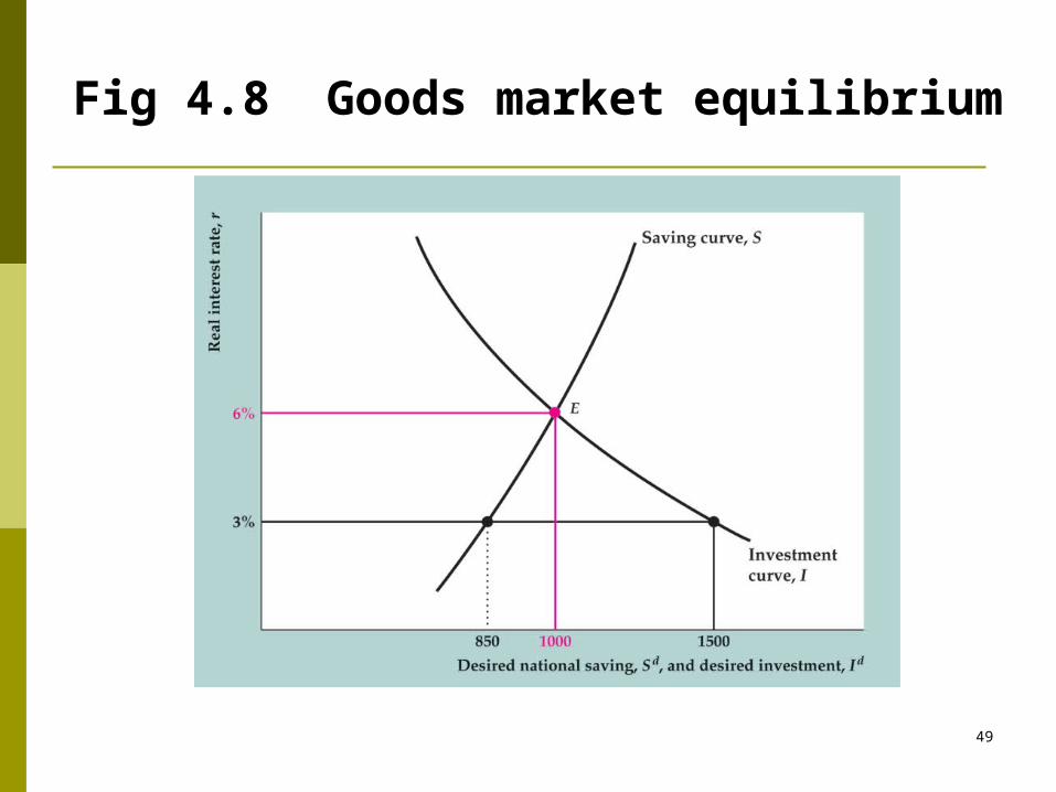
49

Fig 4.8 Goods market equilibrium

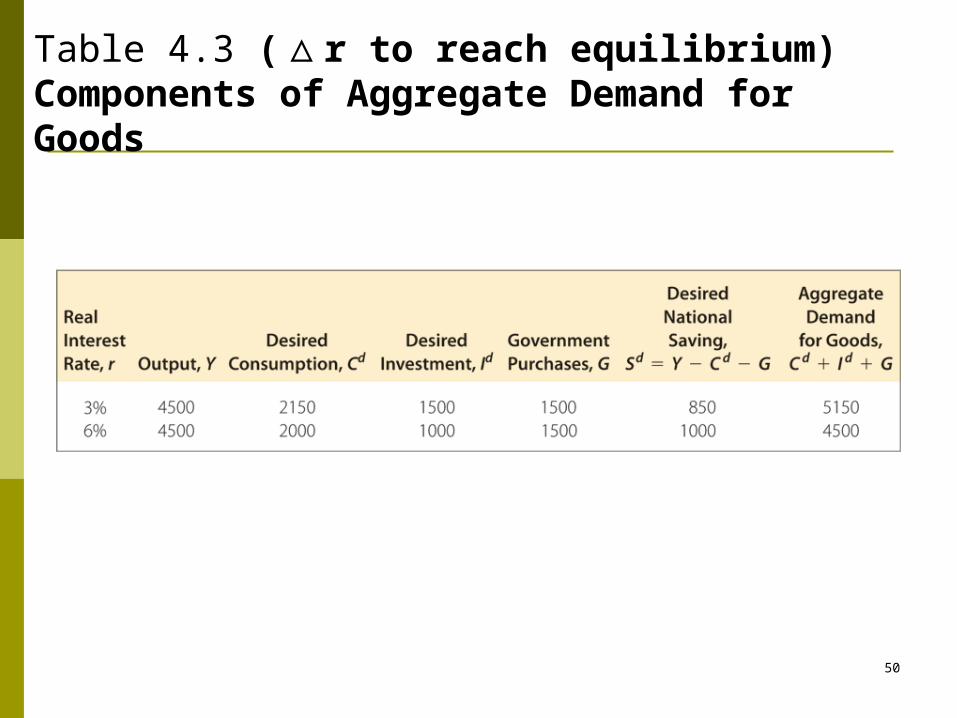
50

Table 4.3 ( r to reach equilibrium△ ) Components of Aggregate Demand for Goods

51

Shifts of the saving curve

Y ?, expected Yf ?, wealth ?, G ?, T ? (unless Ricardian equivalence holds)

Sd↑: Saving curve shifts right

Example: Temporary G↑(Fig. 4.8) S↓: shifts S left r↑: causing crowding out of I

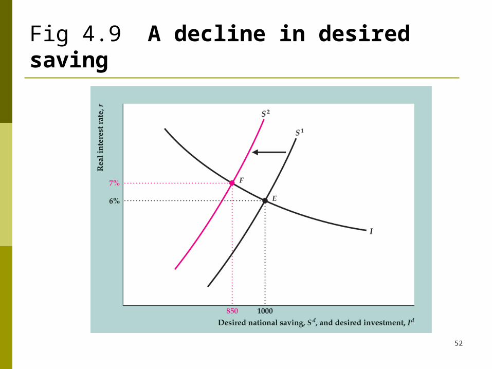
52

Fig 4.9 A decline in desired saving

53

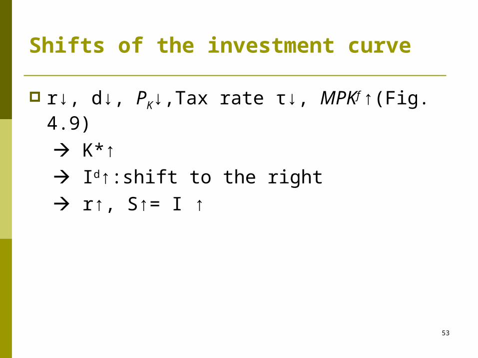
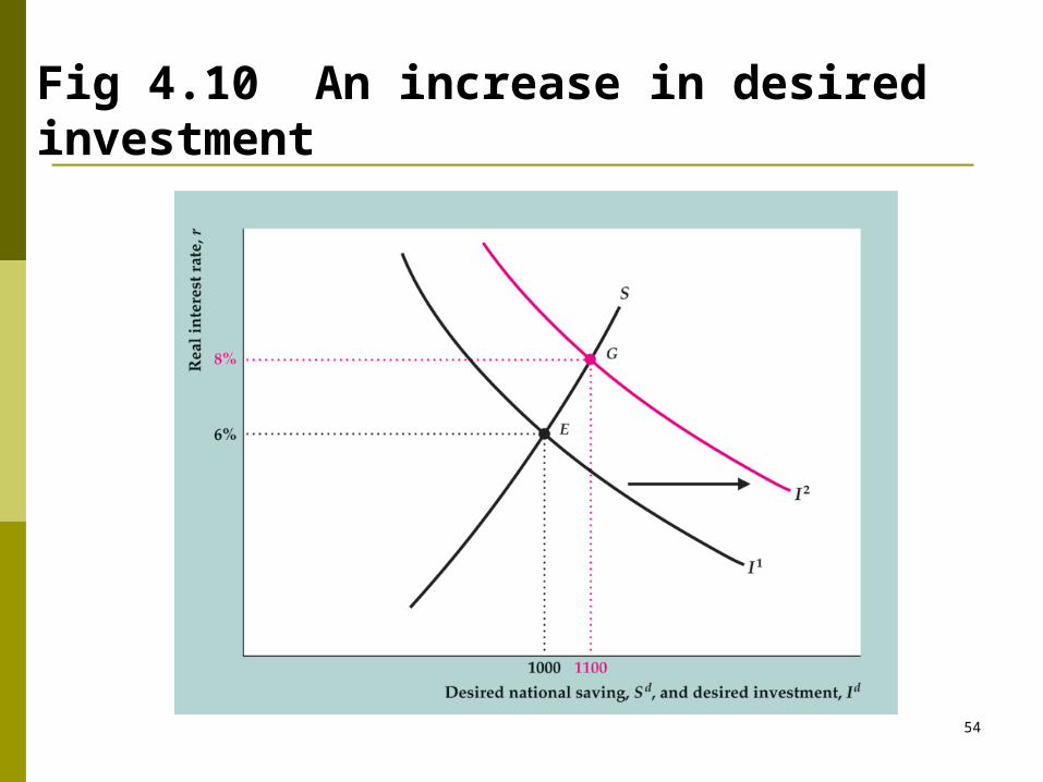
Shifts of the investment curve

r↓, d↓, PK↓,Tax rate τ↓, MPKf ↑(Fig. 4.9)

K*↑

Id↑:shift to the right

r↑, S↑= I ↑

54

Fig 4.10 An increase in desired investment

55

Application: Macroeconomic consequences of the boom and bust in stock prices

Sharp changes in stock prices

affect consumption spending (a wealth effect)

and capital investment (via Tobin’s q) Data in Fig. 4.11

56

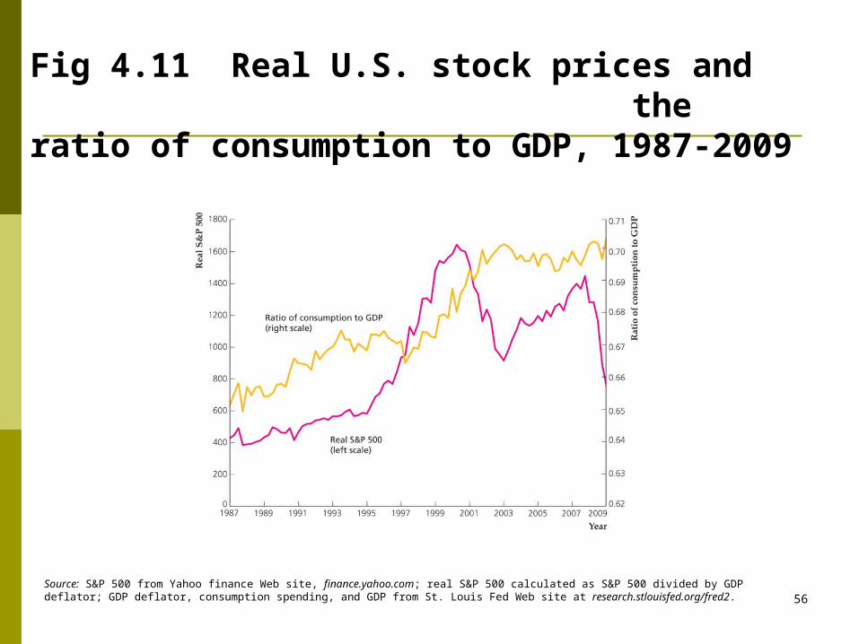
Fig 4.11 Real U.S. stock prices and the ratio of consumption to GDP, 1987-2009

Source: S&P 500 from Yahoo finance Web site, finance.yahoo.com; real S&P 500 calculated as S&P 500 divided by GDP deflator; GDP deflator, consumption spending, and GDP from St. Louis Fed Web site at research.stlouisfed.org/fred2.

57

Consumption and the 1987 crash

When the stock market crashed in 1987, wealth declined by about $1 trillion

Consumption fell somewhat less than might be expected, and it wasn’t enough to cause a recession

There was a temporary decline in confidence about the future, but it was quickly reversed

The small response may have been because there had been a large run-up in stock prices between December 1986 and August 1987, so the crash mostly erased this run-up

58

1987 年美股崩盤重回 1987 年…美股崩盤 相當今跌 3200 點 編譯王錦時／特譯 紐約股市在 1987 年 10 月 19 日當天出現崩盤走勢，道瓊工業平均指數暴跌五○八點，

跌幅高達 22.6 ％。主要是因當時美國的貿易及預算雙赤字攀升至新高峰，引發市場疑慮；同時當天的電腦程式交易，加重了大盤跌勢。

美國在 1987 年的經濟情勢，剛好是 1980 年代經濟繁榮的高峰期。美國已故前總統雷根當時大力推展「供給面經濟學」，實施減稅政策，活絡民間消費及投資，帶動美國經濟強勁擴張。美國股市也自 1982 年開始，展開一波多頭行情。而股市持續上揚自然吸引更多游資聚集，到最後過多的資金在股市瘋狂炒作，漲勢逐漸脫離基本面，形成越來越大的泡沫。而伴隨當時美國經濟景氣擴張而來的是，貿易及預算赤字連袂攀升至新高峰，並引發通膨上揚。

當時美國聯邦準備理事會（ Fed）為抑制通膨，採取升息及緊縮信用的行動，使債券吸引力大幅上升，同時也引發股市投資人對股價高估的疑慮。 10 月 16 日道瓊工業指數已出現重挫 91 點（約 5 ％）的盤勢，同時也有分析師警告指出，紐約股市即將大跌。果然，在 10 月 19 日星期一股市開盤後，龐大的殺盤賣壓有如潮水般湧出，收盤時道瓊工業指數竟暴跌了 508 點；亞洲及歐洲股市也都連鎖遭到波及，應聲劇跌。

當時剛接掌 Fed 主席不久的葛林斯潘，立即發佈強而有力的聲明表示：「聯邦準備體系為支持經濟及金融體系，已經完成提供市場流動性資金的準備。」成功化解了一場全球股市風暴。 1987 年這場股災雖然並未如同 1927 年那次，引發經濟大蕭條。

59

Investment and the declines in the stock market in the 2000s

Investment and Tobin’s q were correlated in 2000 and 2008, when the stock market fell sharply

Investment tended to lag the decline in the stock market, reflecting lags in the process of making investment decisions

The financial crisis of 2008 Stock prices plunged in fall 2008 and early 2009, and

home prices fell sharply as well, leading to a large decline in household net wealth

Despite the decline in wealth, the ratio of consumption to GDP did not decline much

60

Investment and Tobin’s q

Investment and Tobin’s q were not closely correlated following the 1987 crash in stock prices

But the relationship has been tighter in the 1990s and early 2000s, as theory suggests (Fig. 4.11)