Embed Size (px)
Citation preview
ECE 333 © 2002 – 2017 George Gross, University of Illinois at Urbana-Champaign, All Rights Reserved. 1
ECE 333 – GREEN ELECTRIC ENERGY
11. Basic Concepts in Power System Economics
George Gross
Department of Electrical and Computer EngineeringUniversity of Illinois at Urbana–Champaign
ECE 333 © 2002 – 2017 George Gross, University of Illinois at Urbana-Champaign, All Rights Reserved. 2
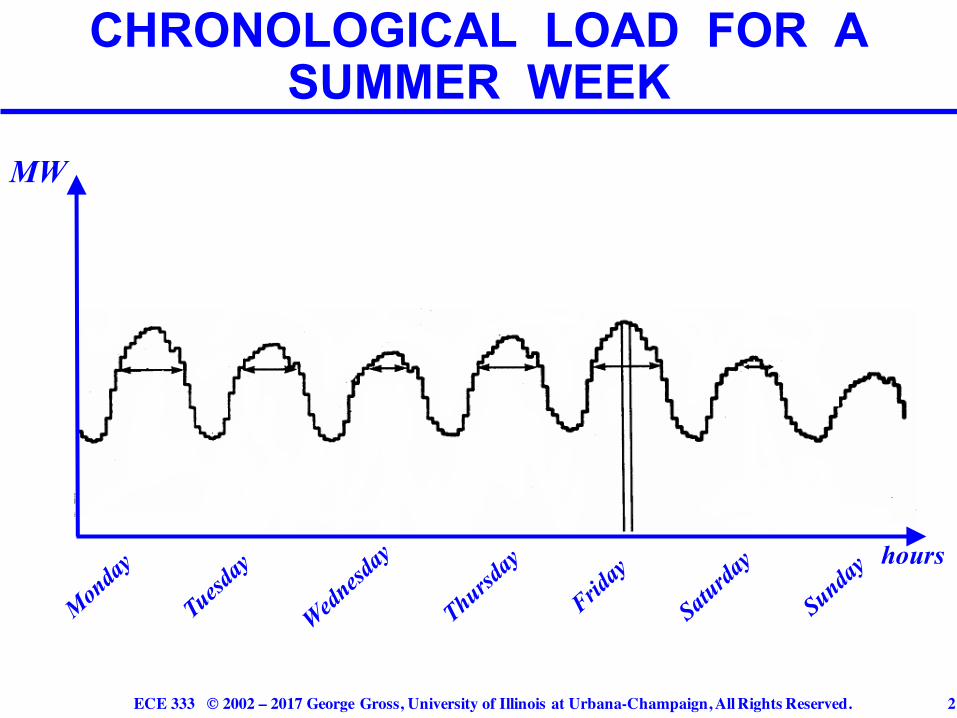
CHRONOLOGICAL LOAD FOR A SUMMER WEEK
MW
hours
ECE 333 © 2002 – 2017 George Gross, University of Illinois at Urbana-Champaign, All Rights Reserved. 3
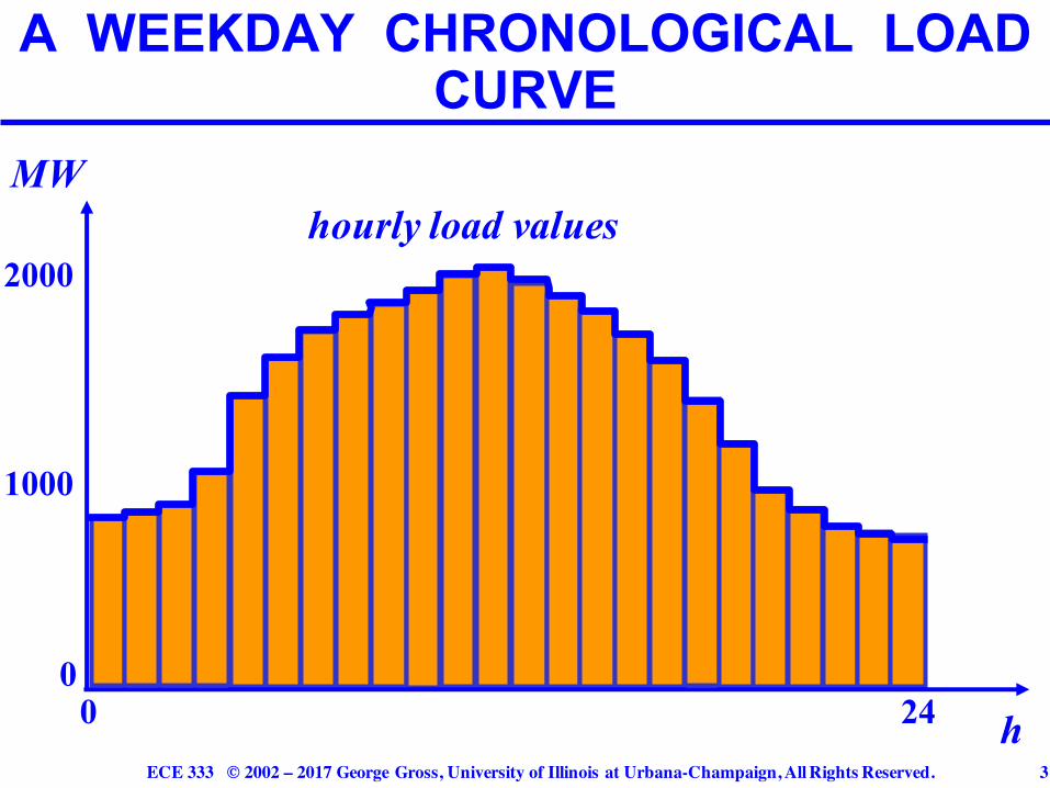
A WEEKDAY CHRONOLOGICAL LOAD CURVE
hourly load valuesMW
2000
0
1000
0 24 h
ECE 333 © 2002 – 2017 George Gross, University of Illinois at Urbana-Champaign, All Rights Reserved. 4
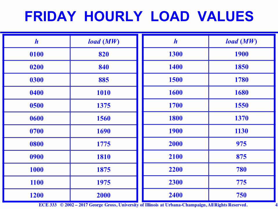
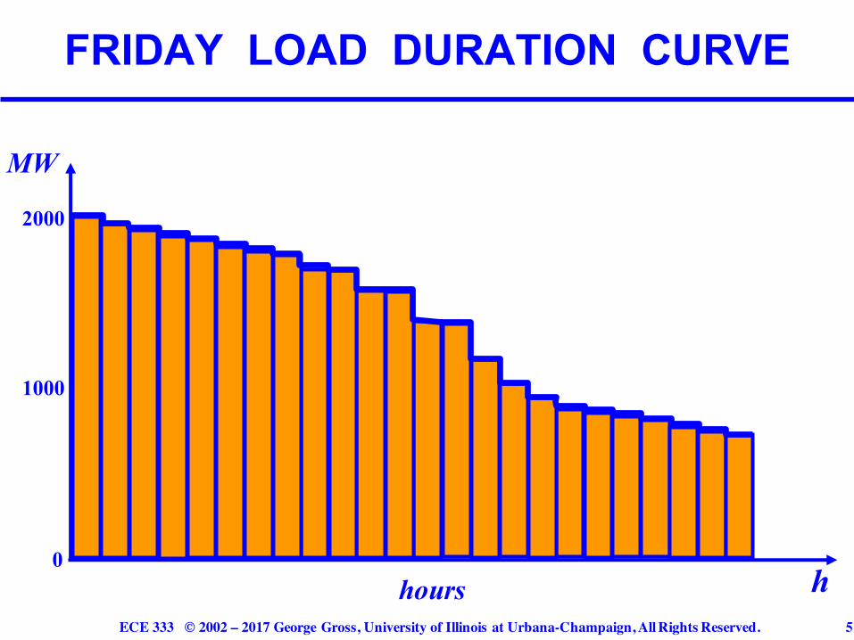
FRIDAY HOURLY LOAD VALUESh load (MW)
0100 820
0200 840
0300 885
0400 1010
0500 1375
0600 1560
0700 1690
0800 1775
0900 1810
1000 1875
1100 1975
1200 2000
h load (MW)
1300 1900
1400 1850
1500 1780
1600 1680
1700 1550
1800 1370
1900 1130
2000 975
2100 875
2200 780
2300 775
2400 750
ECE 333 © 2002 – 2017 George Gross, University of Illinois at Urbana-Champaign, All Rights Reserved. 5
FRIDAY LOAD DURATION CURVE
hours
MW
2000
0
1000
h
ECE 333 © 2002 – 2017 George Gross, University of Illinois at Urbana-Champaign, All Rights Reserved. 6
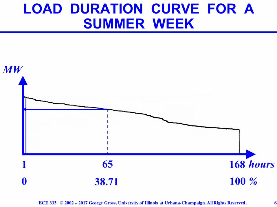
LOAD DURATION CURVE FOR A SUMMER WEEK
MW
138.71
168100 %0
hours65
ECE 333 © 2002 – 2017 George Gross, University of Illinois at Urbana-Champaign, All Rights Reserved. 7
q Inability to m specify the load at any specific hourm distinguish between weekday and weekend
loadsq Ability to
m specify the number of hours at which the load exceeds any given value
m quantify the total energy requirement for the given period in terms of the area under the LDC
LOAD DURATION CURVE CHARACTERISTICS
ECE 333 © 2002 – 2017 George Gross, University of Illinois at Urbana-Champaign, All Rights Reserved. 8
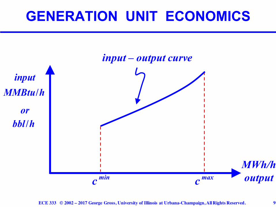
q The costs of generation by a conventional unit
are described by an input-output curve, which
specifies the level of input required to obtain a
required level of output
q Typically, such curves are obtained from actual
measurements and are characterized by their
monotonically non–decreasing shapes
CONVENTIONAL GENERATION UNIT ECONOMICS
ECE 333 © 2002 – 2017 George Gross, University of Illinois at Urbana-Champaign, All Rights Reserved. 9
GENERATION UNIT ECONOMICS
MWh/houtputminc maxc
inputMMBtu/h
orbbl /h
input – output curve
ECE 333 © 2002 – 2017 George Gross, University of Illinois at Urbana-Champaign, All Rights Reserved. 10
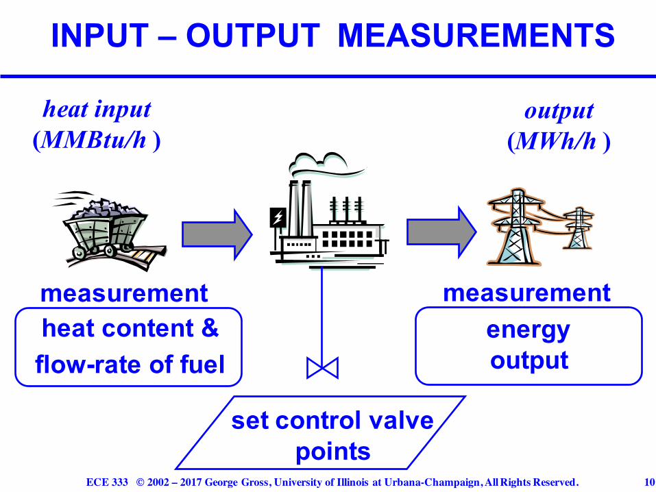
INPUT – OUTPUT MEASUREMENTS
heat input(MMBtu/h )
output (MWh/h )
set control valve points
heat content &flow-rate of fuel
energy output
measurement measurement
ECE 333 © 2002 – 2017 George Gross, University of Illinois at Urbana-Champaign, All Rights Reserved. 11
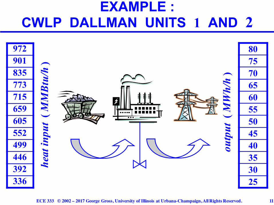
EXAMPLE : CWLP DALLMAN UNITS 1 AND 2
972901835773715659605552499446392336
807570656055504540353025
heat
inpu
t( M
MB
tu/h
)
outp
ut( M
Wh/
h )
ECE 333 © 2002 – 2017 George Gross, University of Illinois at Urbana-Champaign, All Rights Reserved. 12
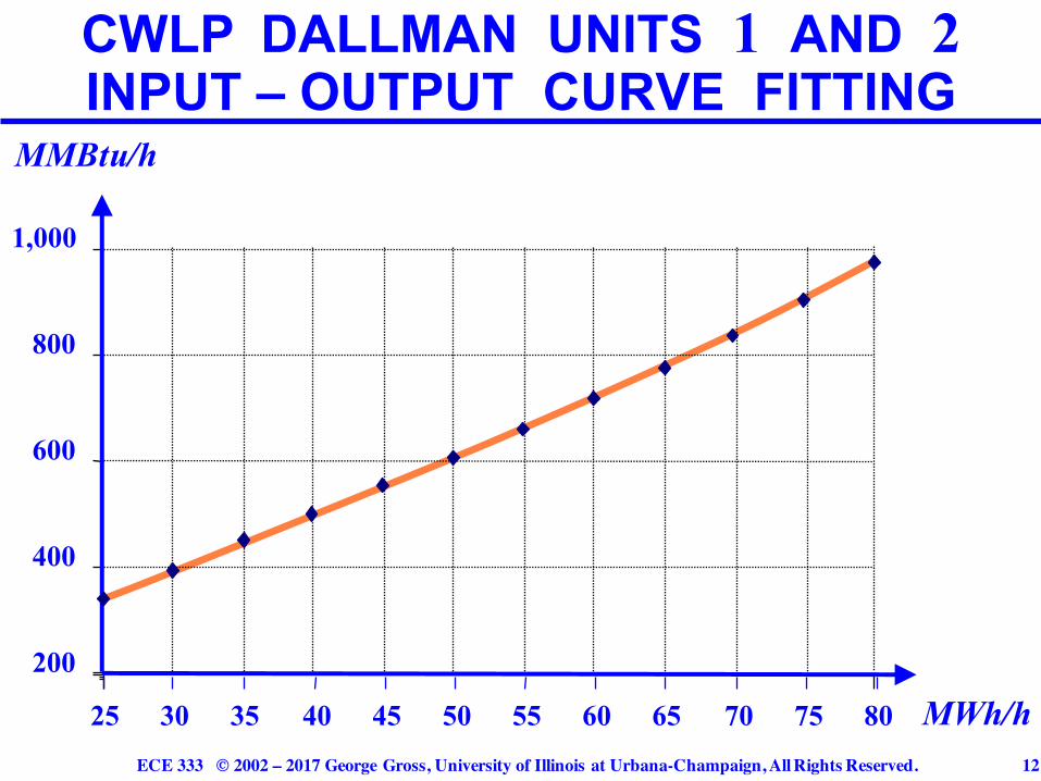
CWLP DALLMAN UNITS 1 AND 2INPUT – OUTPUT CURVE FITTING
MMBtu/h
MWh/h200
400
600
800
1,000
25 30 35 40 45 50 55 60 65 70 75 80
ECE 333 © 2002 – 2017 George Gross, University of Illinois at Urbana-Champaign, All Rights Reserved. 13
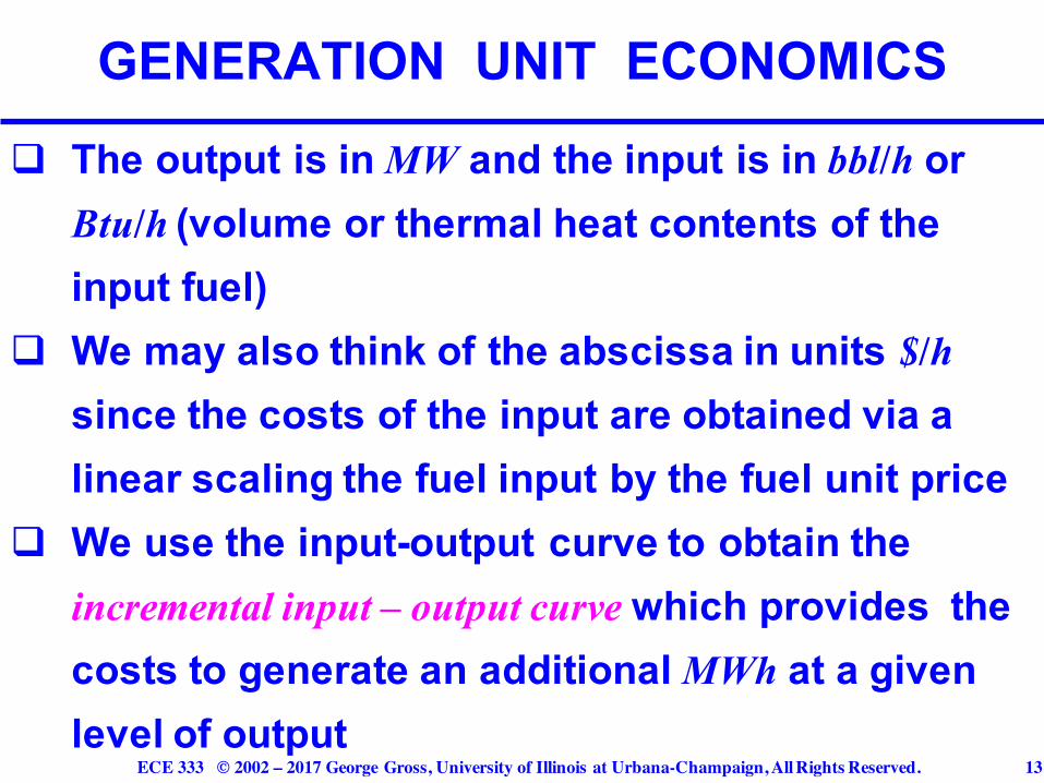
q The output is in MW and the input is in bbl/h or Btu/h (volume or thermal heat contents of the input fuel)
q We may also think of the abscissa in units $/hsince the costs of the input are obtained via a linear scaling the fuel input by the fuel unit price
q We use the input-output curve to obtain the incremental input – output curve which provides the costs to generate an additional MWh at a given level of output
GENERATION UNIT ECONOMICS
ECE 333 © 2002 – 2017 George Gross, University of Illinois at Urbana-Champaign, All Rights Reserved. 14
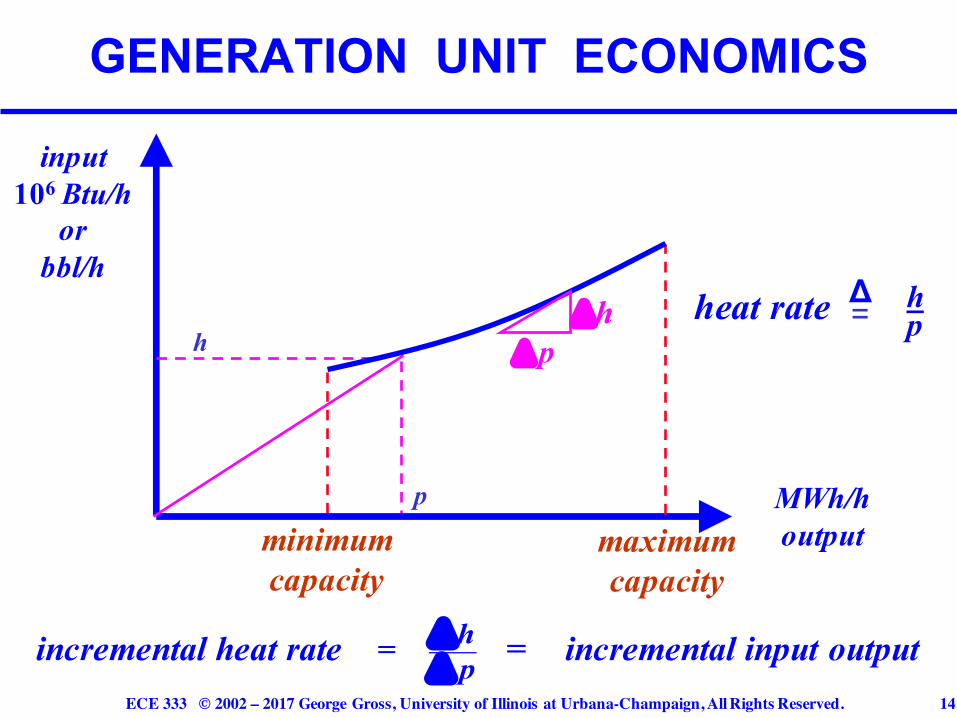
GENERATION UNIT ECONOMICS
incremental heat rate = = incremental input output
heat rate hp=
Δh
p
input 106 Btu/h
orbbl/h
MWh/h outputminimum
capacity
Δh Δ p
maximumcapacity
ΔhΔ p
ECE 333 © 2002 – 2017 George Gross, University of Illinois at Urbana-Champaign, All Rights Reserved. 15
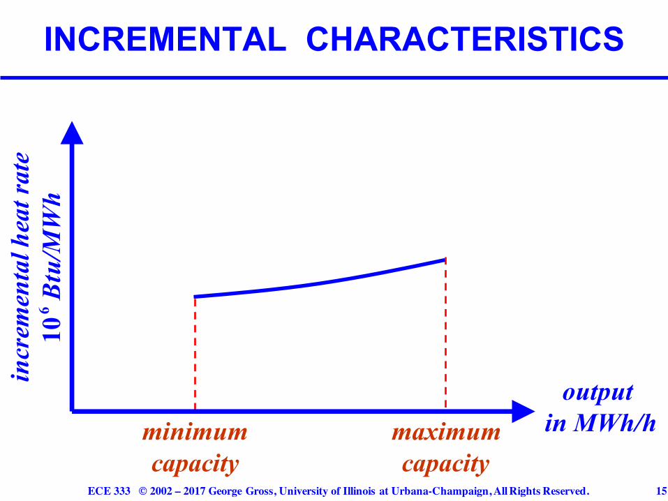
INCREMENTAL CHARACTERISTICS
output in MWh/hminimum
capacitymaximumcapacity
incr
emen
tal h
eat r
ate
106
Btu
/MW
h
ECE 333 © 2002 – 2017 George Gross, University of Illinois at Urbana-Champaign, All Rights Reserved. 16
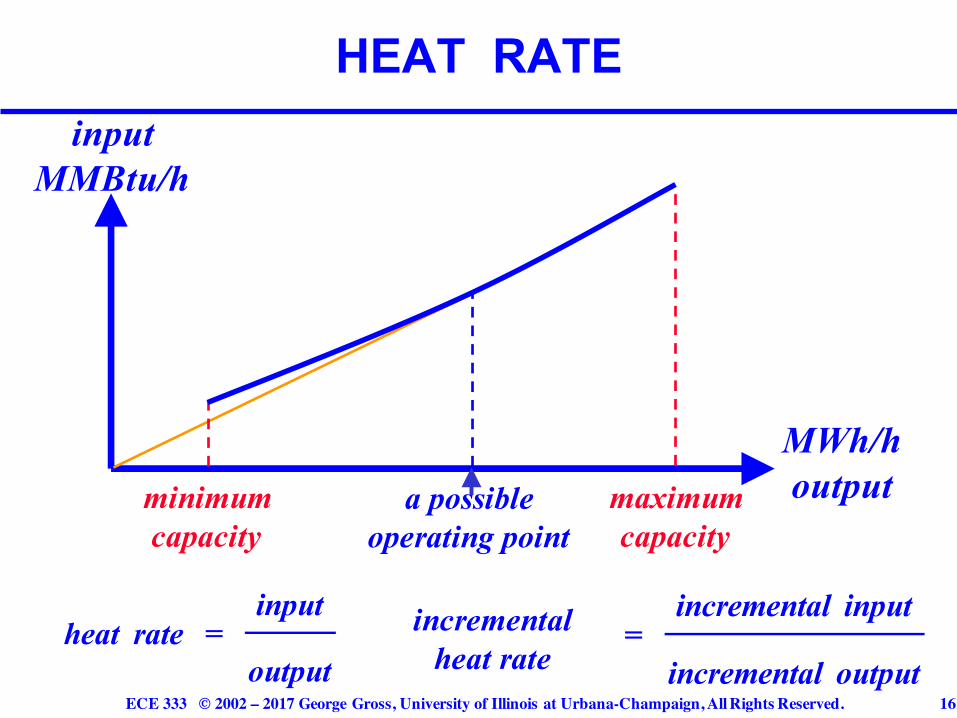
HEAT RATE
a possibleoperating point
MWh/h outputminimum
capacitymaximumcapacity
heat rate =
input
output
incrementalheat rate
=
incremental input
incremental output
input MMBtu/h
ECE 333 © 2002 – 2017 George Gross, University of Illinois at Urbana-Champaign, All Rights Reserved. 17
q The heat rate is a figure of merit widely used by
the industry
q The heat rate gives the inverse of the efficiency
measure of a generation unit since
q The lower the H.R., the higher is the efficiency of
the resource
HEAT RATE
H .R. = input
output
ECE 333 © 2002 – 2017 George Gross, University of Illinois at Urbana-Champaign, All Rights Reserved. 18
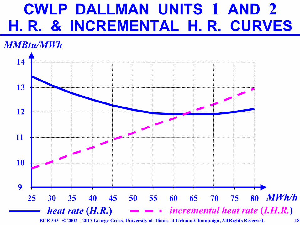
CWLP DALLMAN UNITS 1 AND 2H. R. & INCREMENTAL H. R. CURVES
heat rate (H.R.) incremental heat rate (I.H.R.)
MMBtu/MWh
9
10
11
12
13
14
25 30 35 40 45 50 55 60 65 70 75 80 MWh/h
ECE 333 © 2002 – 2017 George Gross, University of Illinois at Urbana-Champaign, All Rights Reserved. 19
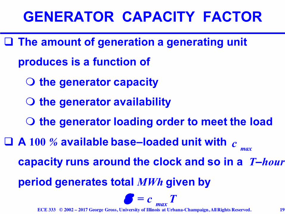
q The amount of generation a generating unit produces is a function of
m the generator capacitym the generator availabilitym the generator loading order to meet the load
q A 100 % available base–loaded unit with capacity runs around the clock and so in a T–hour
period generates total MWh given by
GENERATOR CAPACITY FACTOR
E = c max T
c max
ECE 333 © 2002 – 2017 George Gross, University of Illinois at Urbana-Champaign, All Rights Reserved. 20
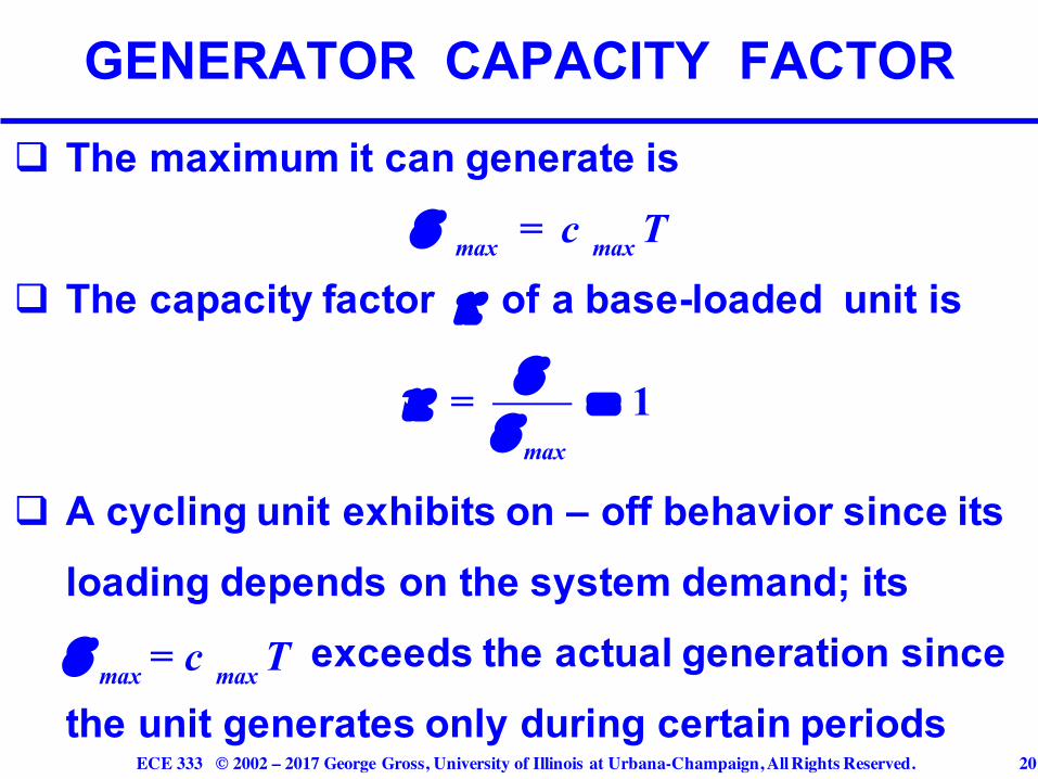
q The maximum it can generate is
q The capacity factor of a base-loaded unit is
q A cycling unit exhibits on – off behavior since its loading depends on the system demand; its
exceeds the actual generation since the unit generates only during certain periods
GENERATOR CAPACITY FACTOR
E max = c max T
κ
κ =
EE max
= 1
E max = c max T
ECE 333 © 2002 – 2017 George Gross, University of Illinois at Urbana-Champaign, All Rights Reserved. 21
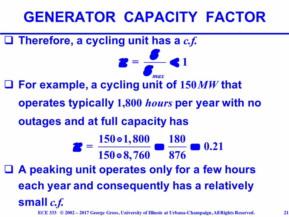
q Therefore, a cycling unit has a c.f.
q For example, a cycling unit of 150MW that operates typically 1,800 hours per year with no outages and at full capacity has
q A peaking unit operates only for a few hours each year and consequently has a relatively small c.f.
GENERATOR CAPACITY FACTOR
κ =
EE max
< 1
κ = 150 ⋅ 1,800
150 ⋅ 8,760= 180
876= 0.21
ECE 333 © 2002 – 2017 George Gross, University of Illinois at Urbana-Champaign, All Rights Reserved. 22
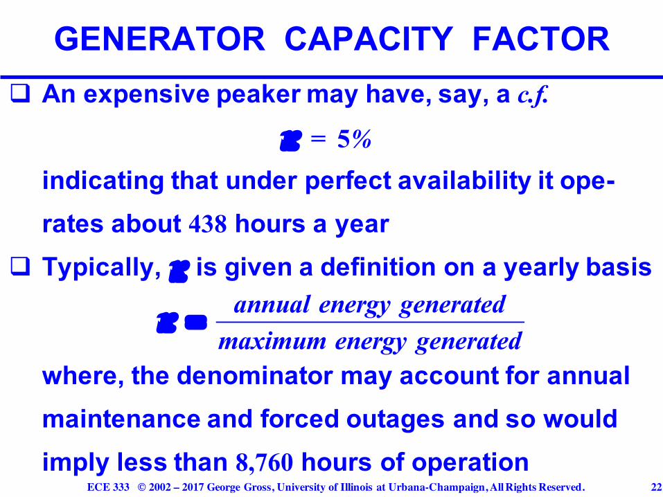
q An expensive peaker may have, say, a c.f.
indicating that under perfect availability it ope-rates about 438 hours a year
q Typically, is given a definition on a yearly basis
where, the denominator may account for annual maintenance and forced outages and so would imply less than 8,760 hours of operation
GENERATOR CAPACITY FACTOR
κ = 5%
κ = annual energy generated
maximum energy generated
κ
ECE 333 © 2002 – 2017 George Gross, University of Illinois at Urbana-Champaign, All Rights Reserved. 23
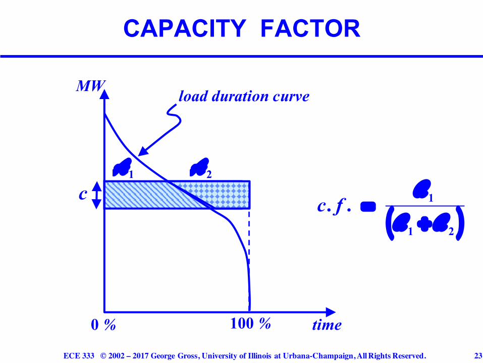
CAPACITY FACTOR
c. f . =
A 1
A 1 + A 2( )
2A1Ac
MW
time0 % 100 %
load duration curve
ECE 333 © 2002 – 2017 George Gross, University of Illinois at Urbana-Champaign, All Rights Reserved. 24
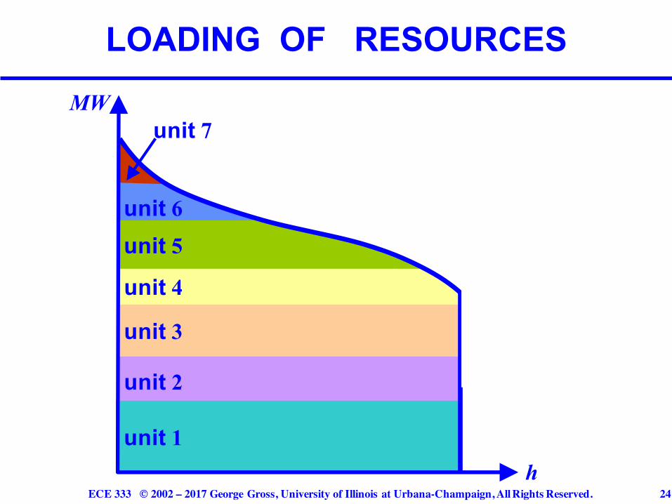
LOADING OF RESOURCES
unit 1
unit 2
unit 3
unit 4
unit 5unit 6
unit 7
h
MW
ECE 333 © 2002 – 2017 George Gross, University of Illinois at Urbana-Champaign, All Rights Reserved. 25
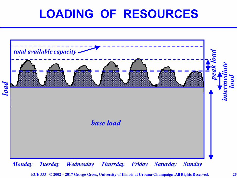
LOADING OF RESOURCES
Monday Tuesday Wednesday Thursday Friday Saturday Sunday
total available capacity
load
inte
rmed
iate
lo
ad
base load
peak
load
ECE 333 © 2002 – 2017 George Gross, University of Illinois at Urbana-Champaign, All Rights Reserved. 26
q Fixed costs are those costs incurred that are
independent of the operation of a resource and
are incurred even if the resource is not operating
q Typical components of fixed costs are:
m investment or capital costs
m insurance
m fixed O&M
m taxes
RESOURCE FIXED AND VARIABLE COSTS
ECE 333 © 2002 – 2017 George Gross, University of Illinois at Urbana-Champaign, All Rights Reserved. 27
q Variable costs are associated with the actual
operation of a resource
q Key components of variable costs are
m fuel costs
m variable O&M
m emission costs
RESOURCE FIXED AND VARIABLE COSTS
ECE 333 © 2002 – 2017 George Gross, University of Illinois at Urbana-Champaign, All Rights Reserved. 28
q The fixed charge rate annualizes the capital costs to
produce a yearly uniform cash–flow set over the
life of a resource
q The annual fixed costs are
q Typically, the yearly charge is given on a per unit
– kW or MW – basis
ANNUALIZED INVESTMENT OR CAPITAL COSTS
yearly costs = fixed costs( ) ⋅ fixed charged rate( )
ECE 333 © 2002 – 2017 George Gross, University of Illinois at Urbana-Champaign, All Rights Reserved. 29
q The fixed charge rate takes into account the
interest on loans, acceptable returns for investors
and other fixed cost components: however, each
component is independent of the generated MWh
q The rate strongly depends on the costs of capital
ANNUALIZED INVESTMENT OR CAPITAL COSTS
ECE 333 © 2002 – 2017 George Gross, University of Illinois at Urbana-Champaign, All Rights Reserved. 30
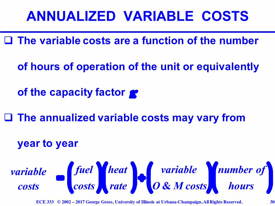
q The variable costs are a function of the number
of hours of operation of the unit or equivalently
of the capacity factor
q The annualized variable costs may vary from
year to year
ANNUALIZED VARIABLE COSTS
variablecosts
=fuelcosts
!
"#
$
%&
heatrate
!
"#
$
%& +
variableO & M costs
!
"#
$
%&
number ofhours
!
"#
$
%&
κ
ECE 333 © 2002 – 2017 George Gross, University of Illinois at Urbana-Champaign, All Rights Reserved. 31
q The yearly variable costs explicitly account for
fuel cost escalation
q Often, the yearly costs are given on a per unit – kW
or MW – basis
q We illustrate these concepts with a pulverized –
coal steam plant
ANNUALIZED VARIABLE COSTS
ECE 333 © 2002 – 2017 George Gross, University of Illinois at Urbana-Champaign, All Rights Reserved. 32
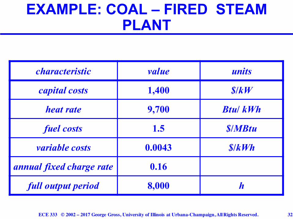
EXAMPLE: COAL – FIRED STEAM PLANT
characteristic value units
capital costs 1,400 $/kW
heat rate 9,700 Btu/ kWh
fuel costs 1.5 $/MBtu
variable costs 0.0043 $/kWh
annual fixed charge rate 0.16
full output period 8,000 h
ECE 333 © 2002 – 2017 George Gross, University of Illinois at Urbana-Champaign, All Rights Reserved. 33
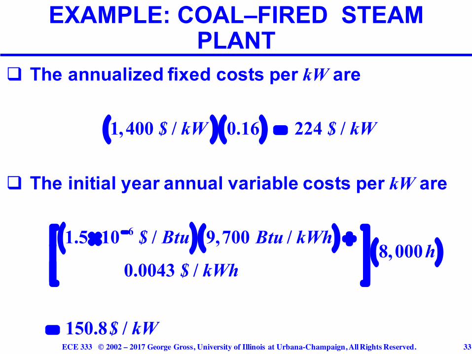
q The annualized fixed costs per kW are
q The initial year annual variable costs per kW are
EXAMPLE: COAL–FIRED STEAM PLANT
1.5×10 −6 $ / Btu( ) 9,700 Btu / kWh( ) +0.0043 $ / kWh
#
$%%
&
'((
8,000h( )
= 150.8$ / kW
1,400 $ / kW( ) 0.16( ) = 224 $ / kW

ECE 333 © 2002 – 2017 George Gross, University of Illinois at Urbana-Champaign, All Rights Reserved. 34
q Total annual costs for 8,000 h are
q Note, we do the example under the assumption of full output for 8,000 h and 0 output for the
remaining 760 h of the yearq We also neglect any possible outages of the unit
and so explicitly ignore any uncertainty in the unit performance
EXAMPLE: COAL–FIRED STEAM PLANT
224 +150.8( )$ / kW8,000 h
= 0.0469 $ / kWh