Embed Size (px)
Citation preview
10. Electroweak model and constraints on new physics 1
10. ELECTROWEAK MODEL AND
CONSTRAINTS ON NEW PHYSICS
Revised December 2011 by J. Erler (U. Mexico and Institute for Advanced Study) andP. Langacker (Princeton University and Institute for Advanced Study).
10.1 Introduction10.2 Renormalization and radiative corrections10.3 Low energy electroweak observables10.4 W and Z boson physics10.5 Precision flavor physics10.6 Experimental results10.7 Constraints on new physics
10.1. Introduction
The standard model of the electroweak interactions (SM) [1] is based on the gaugegroup SU(2) × U(1), with gauge bosons W i
µ, i = 1, 2, 3, and Bµ for the SU(2) andU(1) factors, respectively, and the corresponding gauge coupling constants g andg′. The left-handed fermion fields of the ith fermion family transform as doublets
Ψi =
(νi
ℓ−i
)and
(ui
d′i
)under SU(2), where d′i ≡
∑j Vij dj , and V is the Cabibbo-
Kobayashi-Maskawa mixing matrix. (Constraints on V and tests of universality arediscussed in Ref. 2 and in the Section on “The CKM Quark-Mixing Matrix”. Theextension of the formalism to allow an analogous leptonic mixing matrix is discussed inthe Section on “Neutrino Mass, Mixing, and Oscillations”.) The right-handed fields areSU(2) singlets. In the minimal model there are three fermion families.
A complex scalar Higgs doublet, φ ≡(
φ+
φ0
), is added to the model for mass generation
through spontaneous symmetry breaking with potential∗ given by,
V (φ) = µ2φ†φ +λ2
2(φ†φ)2. (10.1)
For µ2 negative, φ develops a vacuum expectation value, v/√
2, where v ≈ 246.22 GeV,breaking part of the electroweak (EW) gauge symmetry, after which only one neutralHiggs scalar, H, remains in the physical particle spectrum. In non-minimal models thereare additional charged and neutral scalar Higgs particles [3].
After the symmetry breaking the Lagrangian for the fermion fields, ψi, is
LF =∑
i
ψi
(i 6∂ − mi −
gmiH
2MW
)ψi
∗ There is no generally accepted convention to write the quartic term. Our numericalcoefficient simplifies Eq. (10.3a) below and the squared coupling preserves the relation be-tween the number of external legs and the power counting of couplings at a given loop order.This structure also naturally emerges from physics beyond the SM, such as supersymmetry.
J. Beringer et al.(PDG), PR D86, 010001 (2012) (http://pdg.lbl.gov)June 18, 2012 16:19
2 10. Electroweak model and constraints on new physics
− g
2√
2
∑
i
Ψi γµ (1 − γ5)(T+ W+µ + T− W−
µ ) Ψi
− e∑
i
qi ψi γµ ψi Aµ
− g
2 cos θW
∑
i
ψi γµ(giV − gi
Aγ5) ψi Zµ . (10.2)
θW ≡ tan−1(g′/g) is the weak angle; e = g sin θW is the positron electric charge;and A ≡ B cos θW + W 3 sin θW is the photon field (γ). W± ≡ (W 1 ∓ iW 2)/
√2 and
Z ≡ −B sin θW + W 3 cos θW are the charged and neutral weak boson fields, respectively.The Yukawa coupling of H to ψi in the first term in LF , which is flavor diagonal in theminimal model, is gmi/2MW . The boson masses in the EW sector are given (at treelevel, i.e., to lowest order in perturbation theory) by,
MH = λ v, (10.3a)
MW =1
2g v =
e v
2 sin θW, (10.3b)
MZ =1
2
√g2 + g′2 v =
e v
2 sin θW cos θW=
MW
cos θW, (10.3c)
Mγ = 0. (10.3d)
The second term in LF represents the charged-current weak interaction [4–7], whereT+ and T− are the weak isospin raising and lowering operators. For example, thecoupling of a W to an electron and a neutrino is
− e
2√
2 sin θW
[W−
µ e γµ(1 − γ5)ν + W+µ ν γµ (1 − γ5)e
]. (10.4)
For momenta small compared to MW , this term gives rise to the effective four-fermioninteraction with the Fermi constant given by GF /
√2 = 1/2v2 = g2/8M2
W . CP violationis incorporated into the EW model by a single observable phase in Vij .
The third term in LF describes electromagnetic interactions (QED) [8–10], and thelast is the weak neutral-current interaction [5–7]. The vector and axial-vector couplingsare
giV ≡t3L(i) − 2qi sin2 θW , (10.5a)
giA ≡t3L(i), (10.5b)
where t3L(i) is the weak isospin of fermion i (+1/2 for ui and νi; −1/2 for di and ei) andqi is the charge of ψi in units of e.
The first term in Eq. (10.2) also gives rise to fermion masses, and in the presence ofright-handed neutrinos to Dirac neutrino masses. The possibility of Majorana masses isdiscussed in the Section on “Neutrino Mass, Mixing, and Oscillations”.
June 18, 2012 16:19
10. Electroweak model and constraints on new physics 3
10.2. Renormalization and radiative corrections
In addition to the Higgs boson mass, MH , the fermion masses and mixings, and thestrong coupling constant, αs, the SM has three parameters. A particularly useful setcontains the Z mass∗∗, the Fermi constant, and the fine structure constant, which will bediscussed in turn:
The Z boson mass, MZ = 91.1876 ± 0.0021 GeV, has been determined from theZ lineshape scan at LEP 1 [11].
The Fermi constant, GF = 1.1663787(6) × 10−5 GeV−2, is derived from the muonlifetime formula∗∗∗,
~
τµ=
G2F m5
µ
192π3F (ρ)
[1 + H1(ρ)
α(mµ)
π+ H2(ρ)
α2(mµ)
π2
], (10.6)
where ρ = m2e/m2
µ, and where
F (ρ) = 1 − 8ρ + 8ρ3 − ρ4 − 12ρ2 ln ρ = 0.99981295, (10.7a)
H1(ρ) =25
8− π2
2−
(9 + 4π2 + 12 lnρ
)ρ
+ 16π2ρ3/2 + O(ρ2) = −1.80793, (10.7b)
H2(ρ) =156815
5184− 518
81π2 − 895
36ζ(3) +
67
720π4 +
53
6π2 ln 2
− (0.042± 0.002)had − 5
4π2√ρ + O(ρ) = 6.64, (10.7c)
α(mµ)−1 = α−1 +1
3πln ρ + O(α) = 135.901 (10.7d)
The massless corrections to H1 and H2 have been obtained in Refs. 13 and 14, respectively,where the term in parentheses is from the hadronic vacuum polarization [14]. The masscorrections to H1 have been known for some time [15], while those to H2 are morerecent [16]. Notice the term linear in me whose appearance was unforeseen and can betraced to the use of the muon pole mass in the prefactor [16]. The remaining uncertaintyin GF is experimental and has recently been reduced by an order of magnitude by theMuLan collaboration [12] at the PSI.
∗∗ We emphasize that in the fits described in Sec. 10.6 and Sec. 10.7 the values of theSM parameters are affected by all observables that depend on them. This is of no practicalconsequence for α and GF , however, since they are very precisely known.∗∗∗ In the spirit of the Fermi theory, we incorporated the small propagator correction,3/5 m2
µ/M2W , into ∆r (see below). This is also the convention adopted by the MuLan
collaboration [12]. While this breaks with historical consistency, the numerical differencewas negligible in the past.
June 18, 2012 16:19
4 10. Electroweak model and constraints on new physics
The fine structure constant, α = 1/137.035999074(44), is currently dominated bythe e± anomalous magnetic moment [10]. In most EW renormalization schemes, it isconvenient to define a running α dependent on the energy scale of the process, withα−1 ∼ 137 appropriate at very low energy, i.e. close to the Thomson limit. (The runninghas also been observed [17] directly.) For scales above a few hundred MeV this introducesan uncertainty due to the low energy hadronic contribution to vacuum polarization. Inthe modified minimal subtraction (MS) scheme [18] (used for this Review), and withαs(MZ) = 0.120, we have α(mτ )−1 = 133.471 ± 0.014 and α(MZ)−1 = 127.944 ± 0.014.(In this Section we denote quantities defined in the modified minimal subtraction(MS) scheme by a caret; the exception is the strong coupling constant, αs, which willalways correspond to the MS definition and where the caret will be dropped.) Thelatter corresponds to a quark sector contribution (without the top) to the conventional
(on-shell) QED coupling, α(MZ) =α
1 − ∆α(MZ), of ∆α
(5)had(MZ) ≈ 0.02772 ± 0.00010.
These values are updated from Ref. 19 with ∆α(5)had(MZ) moved downwards and its
uncertainty halved (partly due to a more precise charm quark mass). Its correlationwith the µ± anomalous magnetic moment (see Sec. 10.5), as well as the non-linear αs
dependence of α(MZ) and the resulting correlation with the input variable αs, are fullytaken into account in the fits. This is done by using as actual input (fit constraint)
instead of ∆α(5)had(MZ) the analogous low energy contribution by the three light quarks,
∆α(3)had(1.8 GeV) = (55.50 ± 0.78) × 10−4 [20], and by calculating the perturbative and
heavy quark contributions to α(MZ) in each call of the fits according to Ref. 19. Partof the uncertainty (±0.49 × 10⁻⁴) is from e+e− annihilation data below 1.8 GeV and τdecay data (including uncertainties from isospin breaking effects), but uncalculated higherorder perturbative (±0.41× 10⁻⁴) and non-perturbative (±0.44× 10⁻⁴) QCD correctionsand the MS quark mass values (see below) also contribute. Various recent evaluations of
∆α(5)had are summarized in Table 10.1, where the leading order relation† between the MS
and on-shell definitions is given by,
∆α(MZ) − ∆α(MZ) =α
π
(100
27− 1
6− 7
4ln
M2Z
M2W
)≈ 0.0072, (10.8)
and where the first term is from fermions and the other two are from W± loops which areusually excluded from the on-shell definition. Most of the older results relied on e+e− →hadrons cross-section measurements up to energies of 40 GeV, which were somewhathigher than the QCD prediction, suggested stronger running, and were less precise.The most recent results typically assume the validity of perturbative QCD (PQCD) atscales of 1.8 GeV and above, and are in reasonable agreement with each other. There
† Eq. (10.8) is for illustration only. Higher order contributions are directly evaluatedin the MS scheme using the FORTRAN package GAPP [21], including three-loop QEDcontributions of both leptons and quarks. The leptonic three-loop contribution in theon-shell scheme has been obtained in Ref. 22.
June 18, 2012 16:19
10. Electroweak model and constraints on new physics 5
Table 10.1: Recent evaluations of the on-shell ∆α(5)had(MZ). For better comparison
we adjusted central values and errors to correspond to a common and fixed value ofαs(MZ) = 0.120. References quoting results without the top quark decoupled areconverted to the five flavor definition. Ref. [33] uses ΛQCD = 380± 60 MeV; for theconversion we assumed αs(MZ) = 0.118 ± 0.003.
Reference Result Comment
Martin, Zeppenfeld [23] 0.02744 ± 0.00036 PQCD for√
s > 3 GeV
Eidelman, Jegerlehner [24] 0.02803 ± 0.00065 PQCD for√
s > 40 GeV
Geshkenbein, Morgunov [25] 0.02780 ± 0.00006 O(αs) resonance model
Burkhardt, Pietrzyk [26] 0.0280 ± 0.0007 PQCD for√
s > 40 GeV
Swartz [27] 0.02754 ± 0.00046 use of fitting function
Alemany et al. [28] 0.02816 ± 0.00062 incl. τ decay data
Krasnikov, Rodenberg [29] 0.02737 ± 0.00039 PQCD for√
s > 2.3 GeV
Davier & Hocker [30] 0.02784 ± 0.00022 PQCD for√
s > 1.8 GeV
Kuhn & Steinhauser [31] 0.02778 ± 0.00016 complete O(α2s)
Erler [19] 0.02779 ± 0.00020 conv. from MS scheme
Davier & Hocker [32] 0.02770 ± 0.00015 use of QCD sum rules
Groote et al. [33] 0.02787 ± 0.00032 use of QCD sum rules
Martin et al. [34] 0.02741 ± 0.00019 incl. new BES data
Burkhardt, Pietrzyk [35] 0.02763 ± 0.00036 PQCD for√
s > 12 GeV
de Troconiz, Yndurain [36] 0.02754 ± 0.00010 PQCD for s > 2 GeV2
Jegerlehner [37] 0.02765 ± 0.00013 conv. from MOM scheme
Hagiwara et al. [38] 0.02757 ± 0.00023 PQCD for√
s > 11.09 GeV
Burkhardt, Pietrzyk [39] 0.02760 ± 0.00035 incl. KLOE data
Hagiwara et al. [40] 0.02770 ± 0.00022 incl. selected KLOE data
Jegerlehner [41] 0.02755 ± 0.00013 Adler function approach
Davier et al. [20] 0.02750 ± 0.00010 e+e− data
Davier et al. [20] 0.02762 ± 0.00011 incl. τ decay data
Hagiwara et al. [42] 0.02764 ± 0.00014 e+e− data
is, however, some discrepancy between analyses based on e+e− → hadrons cross-sectiondata and those based on τ decay spectral functions [20]. The latter utilize data fromOPAL [43], CLEO [44], ALEPH [45], and Belle [46] and imply lower central values
June 18, 2012 16:19
6 10. Electroweak model and constraints on new physics
for the extracted MH of about 6%. This discrepancy is smaller than in the past and atleast some of it appears to be experimental. The dominant e+e− → π+π− cross-sectionwas measured with the CMD-2 [47] and SND [48] detectors at the VEPP-2M e+e−
collider at Novosibirsk and the results are (after an initial discrepancy due to a flawin the Monte Carlo event generator used by SND) in good agreement with each other.As an alternative to cross-section scans, one can use the high statistics radiative returnevents at e+e− accelerators operating at resonances such as the Φ or the Υ(4S). Themethod [49] is systematics limited but dominates over the Novosibirsk data throughout.The BaBar collaboration [50] studied multi-hadron events radiatively returned fromthe Υ(4S), reconstructing the radiated photon and normalizing to µ±γ final states.Their result is higher compared to VEPP-2M and in fact agrees quite well with the τanalysis including the energy dependence (shape). In contrast, the shape and smalleroverall cross-section from the π+π− radiative return results from the Φ obtained bythe KLOE collaboration [51] differs significantly from what is observed by BaBar. Thediscrepancy originates from the kinematic region
√s& 0.6 GeV, and is most pronounced
for√
s & 0.85 GeV. All measurements including older data [52] and multi-hadron finalstates (there are also discrepancies in the e+e− → 2π+2π− channel [20]) are accountedfor and corrections have been applied for missing channels [20]. Further improvement ofthis dominant theoretical uncertainty in the interpretation of precision data will requirebetter measurements of the cross-section for e+e− → hadrons below the charmoniumresonances including multi-pion and other final states. To improve the precisions inmc(mc) and mb(mb) it would help to remeasure the threshold regions of the heavy quarksas well as the electronic decay widths of the narrow cc and bb resonances.
Further free parameters entering into Eq. (10.2) are the quark and lepton masses,where mi is the mass of the ith fermion ψi. For the quarks these are the current masses.For the light quarks, as described in the note on “Quark Masses” in the Quark Listings,mu = 2.5+0.6
−0.8 MeV, md = 5.0+0.7−0.9 MeV, and ms = 100+30
−20 MeV. These are runningMS masses evaluated at the scale µ = 2 GeV. For the heavier quarks we use QCDsum rule [53] constraints [54] and recalculate their masses in each call of our fits to
account for their direct αs dependence. We find¶, mc(µ = mc) = 1.267+0.032−0.040 GeV and
mb(µ = mb) = 4.197 ± 0.025 GeV, with a correlation of 24%.
The top quark “pole” mass (the quotation marks are a reminder that quarks donot form asymptotic states), mt = 173.4 ± 0.9 GeV, is an average of published andpreliminary CDF and DØ results from run I and II [56] with first results by the CMS [57]and ATLAS [58] collaborations averaged in ignoring correlations. To gauge the possible
¶ Other authors [55] advocate to evaluate and quote mc(µ = 3 GeV) instead. We usemc(µ = mc) because in the global analysis it is convenient to nullify any explicitly mc
dependent logarithms. Note also that our uncertainty for mc (and to a lesser degree formb) is larger than the one in Ref. 55, for example. The reason is that we determinethe continuum contribution for charm pair production using only resonance data andtheoretical consistency across various sum rule moments, and then use any difference to theexperimental continuum data as an additional uncertainty. We also include an uncertaintyfor the condensate terms which grows rapidly for higher moments in the sum rule analysis.
June 18, 2012 16:19
10. Electroweak model and constraints on new physics 7
impact of the neglect of correlations involving the LHC experiments, we also averagedthe results conservatively assuming that the entire 0.75 GeV systematic of the Tevatronaverage is fully correlated with a 0.75 GeV component in both CMS and ATLAS.Incidentally, this yields correlations of similar size as those between the two Tevatronexperiments and the two Runs and reduces the central value by 0.15 GeV. Withinround-off we expect a more refined average to coincide with ours. Our average$ differsslightly from the value, mt = 173.5 ± 0.6 ± 0.8 GeV, which appears in the top quarkListings in this Review and which is based exclusively on published results. We areworking, however, with MS masses in all expressions to minimize theoretical uncertainties.Such a short distance mass definition (unlike the pole mass) is free from non-perturbativeand renormalon [59] uncertainties. We therefore convert to the top quark MS mass,
mt(µ = mt) = mt[1 − 4
3
αs
π+ O(α2
s)], (10.9)
using the three-loop formula [60]. This introduces an additional uncertainty which weestimate to 0.5 GeV (the size of the three-loop term) and add in quadrature to theexperimental pole mass error. This is convenient because we use the pole mass as anexternal constraint while fitting to the MS mass. We are assuming that the kinematic massextracted from the collider events corresponds within this uncertainty to the pole mass.Using the BLM optimized [61] version of the two-loop perturbative QCD formula [62] (aswe did in previous editions of this Review) gives virtually identical results. In summary,we will use mt = 173.4 ± 0.9 (exp.) ± 0.5 (QCD) GeV = 173.4 ± 1.0 GeV (together withMH = 117 GeV) for the numerical values quoted in Sec. 10.2–Sec. 10.5.
sin2 θW and MW can be calculated from MZ , α(MZ), and GF , when values for mt
and MH are given; conversely (as is done at present), MH can be constrained by sin2 θW
and MW . The value of sin2 θW is extracted from neutral-current processes (see Sec. 10.3)and Z pole observables (see Sec. 10.4) and depends on the renormalization prescription.There are a number of popular schemes [63–70] leading to values which differ by smallfactors depending on mt and MH . The notation for these schemes is shown in Table 10.2.
(i) The on-shell scheme [63] promotes the tree-level formula sin2 θW = 1 − M2W /M2
Z to
a definition of the renormalized sin2 θW to all orders in perturbation theory, i.e.,sin2 θW → s2
W ≡ 1 − M2W /M2
Z :
MW =A0
sW (1 − ∆r)1/2, MZ =
MW
cW, (10.10)
where cW ≡ cos θW , A0 = (πα/√
2GF )1/2 = 37.28039(1) GeV, and ∆r includesthe radiative corrections relating α, α(MZ), GF , MW , and MZ . One finds∆r ∼ ∆r0 − ρt/ tan2 θW , where ∆r0 = 1 − α/α(MZ) = 0.06635(10) is due to the
$ At the time of writing this review, the efforts to establish a top quark averaging groupinvolving both the Tevatron and the LHC were still in progress. Therefore we perform asimplified average ourselves.
June 18, 2012 16:19

8 10. Electroweak model and constraints on new physics
Table 10.2: Notations used to indicate the various schemes discussed in the text.Each definition of sin2 θW leads to values that differ by small factors depending onmt and MH . Approximate values are also given for illustration.
Scheme Notation Value
On-shell s2W 0.2231
NOV s2MZ
0.2310
MS s2Z 0.2312
MS ND s2ND 0.2314
Effective angle s2f 0.2315
running of α, and ρt = 3GF m2t /8
√2π2 = 0.00943 (mt/173.4 GeV)2 represents the
dominant (quadratic) mt dependence. There are additional contributions to ∆rfrom bosonic loops, including those which depend logarithmically on MH . Onehas ∆r = 0.0358 ∓ 0.0004 ± 0.00010, where the first uncertainty is from mt andthe second is from α(MZ). Thus the value of s2
W extracted from MZ includes anuncertainty (∓0.00012) from the currently allowed range of mt. This scheme issimple conceptually. However, the relatively large (∼ 3%) correction from ρt causeslarge spurious contributions in higher orders.
(ii) A more precisely determined quantity s2MZ
[64] can be obtained from MZ by
removing the (mt, MH) dependent term from ∆r [65], i.e.,
s2MZ
(1 − s2MZ
) ≡ πα(MZ)√2GF M2
Z
. (10.11)
Using α(MZ)−1 = 128.93 ± 0.02 yields s2MZ
= 0.23102 ∓ 0.00005. The small
uncertainty in s2MZ
compared to other schemes is because the mt dependence has
been removed by definition. However, the mt uncertainty reemerges when otherquantities (e.g., MW or other Z pole observables) are predicted in terms of MZ .
Both s2W and s2
MZdepend not only on the gauge couplings but also on the spontaneous-
symmetry breaking, and both definitions are awkward in the presence of any extension ofthe SM which perturbs the value of MZ (or MW ). Other definitions are motivated by thetree-level coupling constant definition θW = tan−1(g′/g):
(iii) In particular, the modified minimal subtraction (MS) scheme introduces the quantitysin2 θW (µ) ≡ g ′2(µ)/
[g 2(µ) + g ′2(µ)
], where the couplings g and g′ are defined by
modified minimal subtraction and the scale µ is conveniently chosen to be MZ formany EW processes. The value of s 2
Z = sin2 θW (MZ) extracted from MZ is less
sensitive than s2W to mt (by a factor of tan2 θW ), and is less sensitive to most types of
new physics than s2W or s2
MZ. It is also very useful for comparing with the predictions
June 18, 2012 16:19
10. Electroweak model and constraints on new physics 9
of grand unification. There are actually several variant definitions of sin2 θW (MZ),differing according to whether or how finite α ln(mt/MZ) terms are decoupled(subtracted from the couplings). One cannot entirely decouple the α ln(mt/MZ)terms from all EW quantities because mt ≫ mb breaks SU(2) symmetry. Thescheme that will be adopted here decouples the α ln(mt/MZ) terms from the γ–Zmixing [18,66], essentially eliminating any ln(mt/MZ) dependence in the formulaefor asymmetries at the Z pole when written in terms of s 2
Z . (A similar definition isused for α.) The various definitions are related by
s 2Z = c (mt, MH)s2
W = c (mt, MH) s2MZ
, (10.12)
where c = 1.0362 ± 0.0004 and c = 1.0009 ∓ 0.0002. The quadratic mt dependenceis given by c ∼ 1 + ρt/ tan2 θW and c ∼ 1 − ρt/(1 − tan2 θW ), respectively. Theexpressions for MW and MZ in the MS scheme are
MW =A0
sZ(1 − ∆rW )1/2, MZ =
MW
ρ 1/2 cZ
, (10.13)
and one predicts ∆rW = 0.06951 ± 0.00001 ± 0.00010. ∆rW has no quadratic mt
dependence, because shifts in MW are absorbed into the observed GF , so that theerror in ∆rW is dominated by ∆r0 = 1− α/α(MZ) which induces the second quoteduncertainty. The quadratic mt dependence has been shifted into ρ ∼ 1 + ρt, whereincluding bosonic loops, ρ = 1.01051 ± 0.00011. Quadratic MH effects are deferredto two-loop order, while the leading logarithmic MH effect is a good approximationonly for large MH values which are clearly disfavored by the precision data. As anillustration, the shift in MW due to a large MH (for fixed MZ) is given by
∆HMW = −11
96
α
π
MW
c2W − s2W
lnM2
H
M2W
+ O(α2)
∼ −200 MeV (for MH = 10 MW ). (10.14)
(iv) A variant MS quantity s 2ND (used in the 1992 edition of this Review) does not
decouple the α ln(mt/MZ) terms [67]. It is related to s 2Z by
s 2Z = s 2
ND/(1 +
α
πd), (10.15a)
d =1
3
(1
s 2− 8
3
) [(1 +
αs
π) ln
mt
MZ− 15αs
8π
], (10.15b)
Thus, s 2Z − s 2
ND ≈ −0.0002.
(v) Yet another definition, the effective angle [68–70] s2f for the Z vector coupling to
fermion f , is based on Z pole observables and described below.
Experiments are at such level of precision that complete O(α) radiative correctionsmust be applied. For neutral-current and Z pole processes, these corrections areconveniently divided into two classes:
June 18, 2012 16:19
10 10. Electroweak model and constraints on new physics
1. QED diagrams involving the emission of real photons or the exchange of virtualphotons in loops, but not including vacuum polarization diagrams. These graphsoften yield finite and gauge-invariant contributions to observable processes. However,they are dependent on energies, experimental cuts, etc., and must be calculatedindividually for each experiment.
2. EW corrections, including γγ, γZ, ZZ, and WW vacuum polarization diagrams, aswell as vertex corrections, box graphs, etc., involving virtual W and Z bosons. Theone-loop corrections are included for all processes, and certain two-loop correctionsare also important. In particular, two-loop corrections involving the top quarkmodify ρt in ρ, ∆r, and elsewhere by
ρt → ρt[1 + R(MH , mt)ρt/3]. (10.16)
R(MH , mt) is best described as an expansion in M2Z/m2
t . The unsuppressed termswere first obtained in Ref. 71, and are known analytically [72]. Contributionssuppressed by M2
Z/m2t were first studied in Ref. 73 with the help of small and large
Higgs mass expansions, which can be interpolated. These contributions are aboutas large as the leading ones in Refs. 71 and 72. The complete two-loop calculationof ∆r (without further approximation) has been performed in Refs. 74 and 75 forfermionic and purely bosonic diagrams, respectively. Similarly, the EW two-loopcalculation for the relation between s2
ℓ and s2W is complete [76] including the recently
obtained purely bosonic contribution [77]. For MH above its lower direct limit,−17 < R ≤ −13.
Mixed QCD-EW contributions to gauge boson self-energies of order ααsm2t [78]
and αα2sm
2t [79] increase the predicted value of mt by 6%. This is, however,
almost entirely an artifact of using the pole mass definition for mt. The equivalentcorrections when using the MS definition mt(mt) increase mt by less than 0.5%.The subleading ααs corrections [80] are also included. Further three-loop correctionsof order αα2
s [81], α3m6t [82,83], and α2αsm
4t (for MH = 0) [82], are rather
small. The same is true for α3M4H [84] corrections unless MH approaches 1 TeV.
Also known are the singlet contributions (pure gluonic intermediate states) of orderαα2
s [85] and αα3s [86]. Recently, the corresponding non-singlet contributions have
been computed as well [87].
The leading EW two-loop terms for the Z → bb-vertex of O(α2m4t ) have been
obtained in Refs. 71 and 72, and the mixed QCD-EW contributions in Refs. 88and 89. The authors of Ref. 90 completed the two-loop EW fermionic correctionsto s2
b . The O(ααs)-vertex corrections involving massless quarks [91] add coherently,resulting in a sizable effect and shift αs(MZ) when extracted from Z lineshapeobservables (see Sec. 10.4) by ≈ +0.0007.
Many of the EW corrections are absorbed into the renormalized Fermi constantdefined in Eq. (10.6). Others modify the tree-level expressions for Z pole observablesand neutral-current amplitudes. In particular, the relations in Eq. (10.5) now read,
gfV =
√ρf (t
(f)3L − 2qfκf sin2 θW ), g
fA =
√ρf t
(f)3L , (10.17)
June 18, 2012 16:19

10. Electroweak model and constraints on new physics 11
where the EW radiative corrections have been absorbed into corrections ρf − 1and κf − 1, which depend on the fermion f and on the renormalization scheme.In the on-shell scheme, the quadratic mt dependence is given by ρf ∼ 1 + ρt,
κf ∼ 1 + ρt/ tan2 θW , while in MS, ρf ∼ κf ∼ 1, for f 6= b (ρb ∼ 1 − 43ρt,
κb ∼ 1 + 23ρt). In the MS scheme the normalization is changed according
to GF M2Z/2
√2π → α/4s 2
Z c 2Z . (If one continues to normalize amplitudes by
GF M2Z/2
√2π, as in the 1996 edition of this Review, then ρf contains an additional
factor of ρ(1−∆rW )α/α.) In practice, additional bosonic and fermionic loops, vertexcorrections, leading higher order contributions, etc., must be included. For example,in the MS scheme one has ρℓ = 0.9981, κℓ = 1.0013, ρb = 0.9869, and κb = 1.0067. Itis convenient to define an effective angle s2
f ≡ sin2 θWf ≡ κf s 2Z = κf s2
W , in terms
of which gfV and g
fA are given by
√ρf times their tree-level formulae. Because gℓ
V is
very small, not only A0LR = Ae, A
(0,ℓ)FB , and Pτ , but also A
(0,b)FB , A
(0,c)FB , A
(0,s)FB , and
the hadronic asymmetries are mainly sensitive to s2ℓ . One finds that κf (f 6= b) is
almost independent of (mt, MH), so that one can write
s2ℓ ∼ s 2
Z + 0.00029 . (10.18)
Thus, the asymmetries determine values of s2ℓ and s 2
Z almost independent of mt,while the κ’s for the other schemes are mt dependent.
Throughout this Review we utilize EW radiative corrections from the programGAPP [21], which works entirely in the MS scheme, and which is independent of thepackage ZFITTER [70]. Another resource is the recently developed modular fittingtoolkit Gfitter [92].
10.3. Low energy electroweak observables
In the following we discuss EW precision observables obtained at low momentumtransfers [6], i.e. Q2 ≪ M2
Z . It is convenient to write the four-fermion interactionsrelevant to ν-hadron, ν-e, as well as parity violating e-hadron and e-e neutral-currentprocesses in a form that is valid in an arbitrary gauge theory (assuming masslessleft-handed neutrinos). One has,
−Lνh =
GF√2
ν γµ(1 − γ5)ν
×∑
i
[ǫL(i)qi γµ(1 − γ5)qi + ǫR(i)qi γµ(1 + γ5)qi], (10.19)
−Lνe =
GF√2
νµγµ(1 − γ5)νµ e γµ(gνeV − gνe
A γ5)e, (10.20)
−Leh = − GF√
2
∑
i
[C1i e γµγ5e qi γµqi + C2i e γµe qi γµγ5qi
], (10.21)
June 18, 2012 16:19
12 10. Electroweak model and constraints on new physics
−Lee = − GF√
2C2e e γµγ5e e γµe, (10.22)
where one must include the charged-current contribution for νe-e and νe-e and theparity-conserving QED contribution for electron scattering.
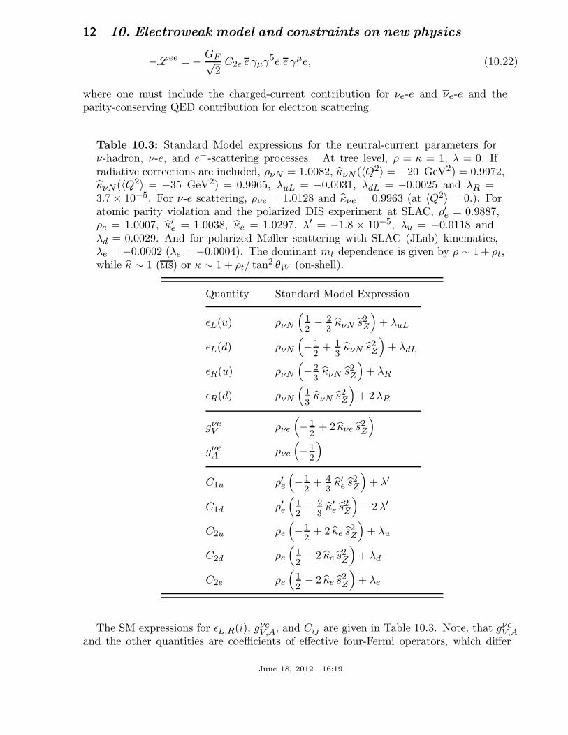
Table 10.3: Standard Model expressions for the neutral-current parameters forν-hadron, ν-e, and e−-scattering processes. At tree level, ρ = κ = 1, λ = 0. Ifradiative corrections are included, ρνN = 1.0082, κνN (〈Q2〉 = −20 GeV2) = 0.9972,κνN (〈Q2〉 = −35 GeV2) = 0.9965, λuL = −0.0031, λdL = −0.0025 and λR =3.7 × 10⁻⁵. For ν-e scattering, ρνe = 1.0128 and κνe = 0.9963 (at 〈Q2〉 = 0.). Foratomic parity violation and the polarized DIS experiment at SLAC, ρ′e = 0.9887,ρe = 1.0007, κ′e = 1.0038, κe = 1.0297, λ′ = −1.8 × 10⁻⁵, λu = −0.0118 andλd = 0.0029. And for polarized Møller scattering with SLAC (JLab) kinematics,λe = −0.0002 (λe = −0.0004). The dominant mt dependence is given by ρ ∼ 1 + ρt,while κ ∼ 1 (MS) or κ ∼ 1 + ρt/ tan2 θW (on-shell).
Quantity Standard Model Expression
ǫL(u) ρνN
(12− 2
3κνN s2
Z
)+ λuL
ǫL(d) ρνN
(− 1
2+ 1
3κνN s2
Z
)+ λdL
ǫR(u) ρνN
(− 2
3κνN s2
Z
)+ λR
ǫR(d) ρνN
(13
κνN s2Z
)+ 2 λR
gνeV ρνe
(− 1
2+ 2 κνe s2
Z
)
gνeA ρνe
(− 1
2
)
C1u ρ′e
(− 1
2+ 4
3κ′e s2
Z
)+ λ′
C1d ρ′e
(12− 2
3κ′e s2
Z
)− 2 λ′
C2u ρe
(− 1
2+ 2 κe s2
Z
)+ λu
C2d ρe
(12− 2 κe s2
Z
)+ λd
C2e ρe
(12− 2 κe s2
Z
)+ λe
The SM expressions for ǫL,R(i), gνeV,A, and Cij are given in Table 10.3. Note, that gνe
V,Aand the other quantities are coefficients of effective four-Fermi operators, which differ
June 18, 2012 16:19
10. Electroweak model and constraints on new physics 13
from the quantities defined in Eq. (10.5) in the radiative corrections and in the presenceof possible physics beyond the SM.
10.3.1. Neutrino scattering : For a general review on ν-scattering we refer to Ref. 93(nonstandard neutrino scattering interactions are surveyed in Ref. 94).
The cross-section in the laboratory system for νµe → νµe or νµe → νµe elasticscattering [95] is
dσν,ν
dy=
G2F meEν
2π
[(gνe
V ± gνeA )2 + (gνe
V ∓ gνeA )2(1 − y)2 − (gνe2
V − gνe2A )
y me
Eν
], (10.23)
where the upper (lower) sign refers to νµ(νµ), and y ≡ Te/Eν (which runs from 0 to(1 + me/2Eν)−1) is the ratio of the kinetic energy of the recoil electron to the incident νor ν energy. For Eν ≫ me this yields a total cross-section
σ =G2
F meEν
2π
[(gνe
V ± gνeA )2 +
1
3(gνe
V ∓ gνeA )2
]. (10.24)
The most accurate measurements [95–100] of sin2 θW from ν-lepton scattering (seeSec. 10.6) are from the ratio R ≡ σνµe/σνµe in which many of the systematic uncertaintiescancel. Radiative corrections (other than mt effects) are small compared to the precisionof present experiments and have negligible effect on the extracted sin2 θW . The mostprecise experiment (CHARM II) [98] determined not only sin2 θW but gνe
V,A as well,which are shown in Fig. 10.1. The cross-sections for νe-e and νe-e may be obtained fromEq. (10.23) by replacing gνe
V,A by gνeV,A + 1, where the 1 is due to the charged-current
contribution.
A precise determination of the on-shell s2W , which depends only very weakly on mt and
MH , is obtained from deep inelastic scattering (DIS) of neutrinos from (approximately)isoscalar targets [101]. The ratio Rν ≡ σNC
νN /σCCνN of neutral-to-charged-current cross-
sections has been measured to 1% accuracy by CDHS [102] and CHARM [103] at CERN.CCFR [104] at Fermilab has obtained an even more precise result, so it is importantto obtain theoretical expressions for Rν and Rν ≡ σNC
νN /σCCνN to comparable accuracy.
Fortunately, many of the uncertainties from the strong interactions and neutrino spectracancel in the ratio. A large theoretical uncertainty is associated with the c-threshold,which mainly affects σCC . Using the slow rescaling prescription [105] the central valueof sin2 θW from CCFR varies as 0.0111(mc [GeV] − 1.31), where mc is the effectivemass which is numerically close to the MS mass mc(mc), but their exact relation isunknown at higher orders. For mc = 1.31±0.24 GeV (determined from ν-induced dimuonproduction [106]) this contributes ±0.003 to the total uncertainty ∆ sin2 θW ∼ ±0.004.(The experimental uncertainty is also ±0.003.) This uncertainty largely cancels, however,in the Paschos-Wolfenstein ratio [107],
R− =σNC
νN − σNCνN
σCCνN − σCC
νN
. (10.25)
June 18, 2012 16:19
14 10. Electroweak model and constraints on new physics
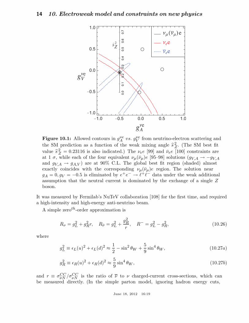
Figure 10.1: Allowed contours in gνeA vs. gνe
V from neutrino-electron scattering and
the SM prediction as a function of the weak mixing angle s 2Z . (The SM best fit
value s 2Z = 0.23116 is also indicated.) The νee [99] and νee [100] constraints are
at 1 σ, while each of the four equivalent νµ(νµ)e [95–98] solutions (gV,A → −gV,Aand gV,A → gA,V ) are at 90% C.L. The global best fit region (shaded) almostexactly coincides with the corresponding νµ(νµ)e region. The solution neargA = 0, gV = −0.5 is eliminated by e+e− → ℓ+ℓ− data under the weak additionalassumption that the neutral current is dominated by the exchange of a single Zboson.
It was measured by Fermilab’s NuTeV collaboration [108] for the first time, and requireda high-intensity and high-energy anti-neutrino beam.
A simple zeroth-order approximation is
Rν = g2L + g2
Rr, Rν = g2L +
g2R
r, R− = g2
L − g2R, (10.26)
where
g2L ≡ ǫL(u)2 + ǫL(d)2 ≈ 1
2− sin2 θW +
5
9sin4 θW , (10.27a)
g2R ≡ ǫR(u)2 + ǫR(d)2 ≈ 5
9sin4 θW , (10.27b)
and r ≡ σCCνN /σCC
νN is the ratio of ν to ν charged-current cross-sections, which canbe measured directly. (In the simple parton model, ignoring hadron energy cuts,
June 18, 2012 16:19
10. Electroweak model and constraints on new physics 15
r ≈ ( 13
+ ǫ)/(1 + 13ǫ), where ǫ ∼ 0.125 is the ratio of the fraction of the nucleon’s
momentum carried by anti-quarks to that carried by quarks.) In practice, Eq. (10.26)must be corrected for quark mixing, quark sea effects, c-quark threshold effects,non-isoscalarity, W–Z propagator differences, the finite muon mass, QED and EWradiative corrections. Details of the neutrino spectra, experimental cuts, x and Q2
dependence of structure functions, and longitudinal structure functions enter only at thelevel of these corrections and therefore lead to very small uncertainties. CCFR quotess2W = 0.2236 ± 0.0041 for (mt, MH) = (175, 150) GeV with very little sensitivity to
(mt, MH).
The NuTeV collaboration found s2W = 0.2277 ± 0.0016 (for the same reference values),
which was 3.0 σ higher than the SM prediction [108]. The deviation was in g2L (initially
2.7 σ low) while g2R was consistent with the SM. Since then a number of experimental and
theoretical developments changed the interpretation of the measured cross section ratios,affecting the extracted g2
L,R (and thus s2W ) including their uncertainties and correlation.
In the following paragraph we give a semi-quantitative and preliminary discussion of theseeffects, but we stress that the precise impact of them needs to be evaluated carefully bythe collaboration with a new and self-consistent set of PDFs, including new radiativecorrections, while simultaneously allowing isospin breaking and asymmetric strange seas.This is an effort which is currently on its way and until it is completed we do not includethe NuTeV constraints on g2
L,R in our default set of fits.
(i) In the original analysis NuTeV worked with a symmetric strange quark seabut subsequently measured [109] the difference between the strange and antistrange
momentum distributions, S− ≡∫ 10 dxx[s(x) − s(x)] = 0.00196 ± 0.00143, from dimuon
events utilizing the first complete next-to-leading order QCD description [110] and partondistribution functions (PDFs) according to Ref. 111. The global PDF fits in Ref. 112give somewhat smaller values, S− = 0.0013(9) [S− = 0.0010(13)], where the semi-leptoniccharmed-hadron branching ratio, Bµ = 8.8 ± 0.5%, has [not] been used as an externalconstraint. The resulting S− also depends on the PDF model used and on whethertheoretical arguments (see Ref. 113 and references therein) are invoked favoring a zerocrossing of x[s(x) − s(x)] at values much larger than seen by NuTeV and suggesting aneffect of much smaller and perhaps negligible size. (ii) The measured branching ratiofor Ke3 decays enters crucially in the determination of the νe(νe) contamination ofthe νµ(νµ) beam. This branching ratio has moved from 4.82 ± 0.06% at the time ofthe original publication [108] to the current value of 5.07 ± 0.04%, i.e., a change bymore than 4 σ. This moves s2
W about one standard deviation further away from theSM prediction while reducing the νe(νe) uncertainty. (iii) PDFs seem to violate isospinsymmetry at levels much stronger than generally expected [114]. A minimum χ2 set ofPDFs [115] allowing charge symmetry violation for both valence quarks [d
pV (x) 6= un
V (x)]and sea quarks [dp(x) 6= un(x)] shows a reduction in the NuTeV discrepancy byabout 1σ. But isospin symmetry violating PDFs are currently not well constrainedphenomenologically and within uncertainties the NuTeV anomaly could be accountedfor in full or conversely made larger [115]. Still, the leading contribution from quarkmass differences turns out to be largely model-independent [116] (at least in sign) and
June 18, 2012 16:19
16 10. Electroweak model and constraints on new physics
a shift, δs2W = −0.0015 ± 0.0003 [113], has been estimated. (iv) QED splitting effects
also violate isospin symmetry with an effect on s2W whose sign (reducing the discrepancy)
is model-independent. The corresponding shift of δs2W = −0.0011 has been calculated in
Ref. 117 but has a large uncertainty. (v) Nuclear shadowing effects [118] are likely toaffect the interpretation of the NuTeV result at some level, but the NuTeV collaborationargues that their data are dominated by values of Q2 at which nuclear shadowing isexpected to be relatively small. However, another nuclear effect, the isovector EMCeffect [119], is much larger (because it affects all neutrons in the nucleus, not just theexcess ones) and model-independently works to reduce the discrepancy. It is estimated tolead to a shift of δs2
W = −0.0019 ± 0.0006 [113]. It would be important to verify andquantify this kind of effect experimentally, e.g., in polarized electron scattering. (vi) Theextracted s2
W may also shift at the level of the quoted uncertainty when analyzed usingthe most recent QED and EW radiative corrections [120,121], as well as QCD correctionsto the structure functions [122]. However, these are scheme-dependent and in order tojudge whether they are significant they need to be adapted to the experimental conditionsand kinematics of NuTeV, and have to be obtained in terms of observable variables andfor the differential cross-sections. In addition, there is the danger of double countingsome of the QED splitting effects. (vii) New physics could also affect g2
L,R [123] but it isdifficult to convincingly explain the entire effect that way.
10.3.2. Parity violation :
The SLAC polarized electron-deuteron DIS experiment [124] measured the right-leftasymmetry,
A =σR − σL
σR + σL, (10.28)
where σR,L is the cross-section for the deep-inelastic scattering of a right- or left-handedelectron: eR,LN → eX. In the quark parton model,
A
Q2= a1 + a2
1 − (1 − y)2
1 + (1 − y)2, (10.29)
where Q2 > 0 is the momentum transfer and y is the fractional energy transfer from theelectron to the hadrons. For the deuteron or other isoscalar targets, one has, neglectingthe s-quark and anti-quarks,
a1 =3GF
5√
2πα
(C1u − 1
2C1d
)≈ 3GF
5√
2πα
(−3
4+
5
3sin2 θW
), (10.30a)
a2 =3GF
5√
2πα
(C2u − 1
2C2d
)≈ 9GF
5√
2πα
(sin2 θW − 1
4
). (10.30b)
In another polarized-electron scattering experiment on deuterons, but in the quasi-elastickinematic regime, the SAMPLE experiment [125] at MIT-Bates extracted the combinationC2u − C2d at Q2 values of 0.1 GeV2 and 0.038 GeV2. What was actually determined
June 18, 2012 16:19
10. Electroweak model and constraints on new physics 17
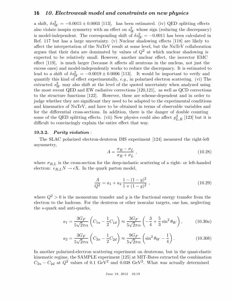
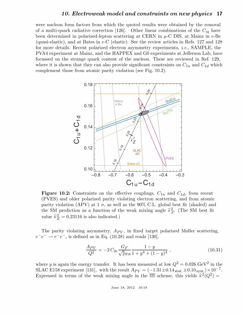
were nucleon form factors from which the quoted results were obtained by the removalof a multi-quark radiative correction [126]. Other linear combinations of the Ciq havebeen determined in polarized-lepton scattering at CERN in µ-C DIS, at Mainz in e-Be(quasi-elastic), and at Bates in e-C (elastic). See the review articles in Refs. 127 and 128for more details. Recent polarized electron asymmetry experiments, i.e., SAMPLE, thePVA4 experiment at Mainz, and the HAPPEX and G0 experiments at Jefferson Lab, havefocussed on the strange quark content of the nucleon. These are reviewed in Ref. 129,where it is shown that they can also provide significant constraints on C1u and C1d whichcomplement those from atomic parity violation (see Fig. 10.2).
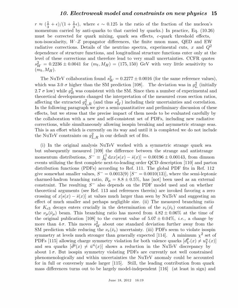
Figure 10.2: Constraints on the effective couplings, C1u and C1d, from recent(PVES) and older polarized parity violating electron scattering, and from atomicparity violation (APV) at 1 σ, as well as the 90% C.L. global best fit (shaded) andthe SM prediction as a function of the weak mixing angle s 2
Z . (The SM best fit
value s 2Z = 0.23116 is also indicated.)
The parity violating asymmetry, APV , in fixed target polarized Møller scattering,e−e− → e−e−, is defined as in Eq. (10.28) and reads [130],
APV
Q2= −2 C2e
GF√2πα
1 − y
1 + y4 + (1 − y)4, (10.31)
where y is again the energy transfer. It has been measured at low Q2 = 0.026 GeV2 in theSLAC E158 experiment [131], with the result APV = (−1.31±0.14 stat.±0.10 syst.)×10−7.Expressed in terms of the weak mixing angle in the MS scheme, this yields s 2(Q2) =
June 18, 2012 16:19

18 10. Electroweak model and constraints on new physics
0.2403 ± 0.0013, and established the scale dependence of the weak mixing angle (seeFig. 10.3) at the level of 6.4 standard deviations. One can also define the so-called weakcharge of the electron (cf. Eq. (10.32) below) as QW (e) ≡ −2 C2e = −0.0403 ± 0.0053(the implications are discussed in Ref. 133).
Figure 10.3: Scale dependence of the weak mixing angle defined in the MS
scheme [132] (for the scale dependence of the weak mixing angle defined in amass-dependent renormalization scheme, see Ref. 133). The minimum of the curvecorresponds to Q = MW , below which we switch to an effective theory with theW± bosons integrated out, and where the β-function for the weak mixing anglechanges sign. At the location of the W boson mass and each fermion mass thereare also discontinuities arising from scheme dependent matching terms which arenecessary to ensure that the various effective field theories within a given looporder describe the same physics. However, in the MS scheme these are very smallnumerically and barely visible in the figure provided one decouples quarks atQ = mq(mq). The width of the curve reflects the theory uncertainty from stronginteraction effects which at low energies is at the level of ±7×10⁻⁵ [132]. Followingthe estimate [135] of the typical momentum transfer for parity violation experimentsin Cs, the location of the APV data point is given by µ = 2.4 MeV. For NuTeV wedisplay the updated value from Ref. 134 and chose µ =
√20 GeV which is about
half-way between the averages of√
Q2 for ν and ν interactions at NuTeV. TheTevatron measurements are strongly dominated by invariant masses of the finalstate dilepton pair of O(MZ) and can thus be considered as additional Z pole datapoints. However, for clarity we displayed the point horizontally to the right. Similarremarks apply to the first measurement at the LHC by the CMS collaboration.
June 18, 2012 16:19
10. Electroweak model and constraints on new physics 19
In a similar experiment and at about the same Q2, Qweak at Jefferson Lab [136] willbe able to measure the weak charge of the proton, QW (p) = −2 [2 C1u +C1d], and sin2 θW
in polarized ep scattering with relative precisions of 4% and 0.3%, respectively.
There are precise experiments measuring atomic parity violation (APV) [137] incesium [138,139] (at the 0.4% level [138]) , thallium [140], lead [141], and bismuth [142].The EW physics is contained in the weak charges which are defined by,
QW (Z, N) ≡ −2 [C1u (2Z + N) + C1d(Z + 2N)] ≈ Z(1 − 4 sin2 θW ) − N. (10.32)
E.g., QW (133Cs) is extracted by measuring experimentally the ratio of the parity violatingamplitude, EPNC, to the Stark vector transition polarizability, β, and by calculatingtheoretically EPNC in terms of QW . One can then write,
QW = N
(ImEPNC
β
)
exp.
( |e| aB
Im EPNC
QW
N
)
th.
(β
a3B
)
exp.+th.
(a2B
|e|
).
The uncertainties associated with atomic wave functions are quite small for cesium [143].The semi-empirical value of β used in early analyses added another source of theoreticaluncertainty [144]. However, the ratio of the off-diagonal hyperfine amplitude to thepolarizability was subsequently measured directly by the Boulder group [145]. Combinedwith the precisely known hyperfine amplitude [146] one finds, β = 26.991 ± 0.046, inexcellent agreement with the earlier results, reducing the overall theory uncertainty(while slightly increasing the experimental error). The recent state-of-the-art many bodycalculation [147] yields, Im EPNC = (0.8906± 0.0026)× 10−11|e| aB QW /N , while the twomeasurements [138,139] combine to give ImEPNC/β = −1.5924 ± 0.0055 mV/cm, andwe obtain QW (13378Cs) = −73.20 ± 0.35. Thus, the various theoretical efforts in Refs. 147and 148 together with an update of the SM calculation [149] including a very recentdispersion analysis of the γZ-box contribution [150] removed an earlier 2.3 σ deviationfrom the SM (see the year 2000 edition of this Review). The theoretical uncertainties are3% for thallium [151] but larger for the other atoms. The Boulder experiment in cesiumalso observed the parity-violating weak corrections to the nuclear electromagnetic vertex(the anapole moment [152]) .
In the future it could be possible to further reduce the theoretical wave functionuncertainties by taking the ratios of parity violation in different isotopes [137,153].There would still be some residual uncertainties from differences in the neutron chargeradii, however [154]. Experiments in hydrogen and deuterium are another possibility forreducing the atomic theory uncertainties [155], while measurements of single trappedradium ions are promising [156] because of the much larger parity violating effect.
June 18, 2012 16:19
20 10. Electroweak model and constraints on new physics
10.4. W and Z boson physics
10.4.1. e+
e− scattering below the Z pole :
The forward-backward asymmetry for e+e− → ℓ+ℓ−, ℓ = µ or τ , is defined as
AFB ≡ σF − σB
σF + σB, (10.33)
where σF (σB) is the cross-section for ℓ− to travel forward (backward) with respect tothe e− direction. AFB and R, the total cross-section relative to pure QED, are given by
R = F1 , AFB =3
4
F2
F1, (10.34)
where
F1 = 1 − 2χ0 geV gℓ
V cos δR + χ20
(ge2V + ge2
A
) (gℓ2V + gℓ2
A
), (10.35a)
F2 = −2χ0 geA gℓ
A cos δR + 4χ20 ge
A gℓA ge
V gℓV , (10.35b)
tan δR =MZΓZ
M2Z − s
, χ0 =GF
2√
2πα
sM2Z[
(M2Z − s)2 + M2
ZΓ2Z
]1/2, (10.36)
and where√
s is the CM energy. Eqs. (10.35) are valid at tree level. If the data areradiatively corrected for QED effects (as described in Sec. 10.2), then the remaining EWcorrections can be incorporated [157,158] (in an approximation adequate for existingPEP, PETRA, and TRISTAN data, which are well below the Z pole) by replacing χ0 byχ(s) ≡ (1 + ρt) χ0(s) α/α(s), where α(s) is the running QED coupling, and evaluating gVin the MS scheme. Reviews and formulae for e+e− → hadrons may be found in Ref. 159.
10.4.2. Z pole physics :
At LEP 1 and the SLC, there were high-precision measurements of various Z poleobservables [11,160–166], as summarized in Table 10.5. These include the Z mass andtotal width, ΓZ , and partial widths Γ(ff) for Z → ff where fermion f = e, µ, τ , hadrons,b, or c. It is convenient to use the variables MZ , ΓZ , Rℓ ≡ Γ(had)/Γ(ℓ+ℓ−) (ℓ = e, µ, τ),σhad ≡ 12π Γ(e+e−) Γ(had)/M2
Z Γ2Z , Rb ≡ Γ(bb)/Γ(had), and Rc ≡ Γ(cc)/Γ(had),
most of which are weakly correlated experimentally. (Γ(had) is the partial widthinto hadrons.) The three values for Rℓ are not inconsistent with lepton universality(although Rτ is somewhat low compared to Re and Rµ), but we use the generalanalysis in which the three observables are treated as independent. Similar remarks
apply to A0,ℓFB defined in Eq. (10.39) (A
0,τFB is somewhat high). O(α3) QED corrections
introduce a large anti-correlation (−30%) between ΓZ and σhad. The anti-correlationbetween Rb and Rc is −18% [11]. The Rℓ are insensitive to mt except for theZ → bb vertex and final state corrections and the implicit dependence through sin2 θW .Thus, they are especially useful for constraining αs. The width for invisible decays [11],
June 18, 2012 16:19
10. Electroweak model and constraints on new physics 21
Γ(inv) = ΓZ−3 Γ(ℓ+ℓ−)−Γ(had) = 499.0±1.5 MeV, can be used to determine the numberof neutrino flavors much lighter than MZ/2, Nν = Γ(inv)/Γtheory(νν) = 2.984± 0.009 for(mt, MH) = (173.4, 117) GeV.
There were also measurements of various Z pole asymmetries. These include thepolarization or left-right asymmetry
ALR ≡ σL − σR
σL + σR, (10.37)
where σL(σR) is the cross-section for a left-(right-)handed incident electron. ALR wasmeasured precisely by the SLD collaboration at the SLC [162], and has the advantages ofbeing extremely sensitive to sin2 θW and that systematic uncertainties largely cancel. Inaddition, SLD extracted the final-state couplings (defined below), Ab, Ac [11], As [163],Aτ , and Aµ [164], from left-right forward-backward asymmetries, using
AFBLR (f) =
σfLF − σ
fLB − σ
fRF + σ
fRB
σfLF + σ
fLB + σ
fRF + σ
fRB
=3
4Af , (10.38)
where, for example, σfLF is the cross-section for a left-handed incident electron to
produce a fermion f traveling in the forward hemisphere. Similarly, Aτ was measured atLEP 1 [11] through the negative total τ polarization, Pτ , and Ae was extracted from theangular distribution of Pτ . An equation such as (10.38) assumes that initial state QEDcorrections, photon exchange, γ–Z interference, the tiny EW boxes, and corrections for√
s 6= MZ are removed from the data, leaving the pure EW asymmetries. This allows theuse of effective tree-level expressions,
ALR = AePe , AFB =3
4Af
Ae + Pe
1 + PeAe, (10.39)
where
Af ≡2gf
V gfA
gf2V + g
f2A
. (10.40)
Pe is the initial e− polarization, so that the second equality in Eq. (10.38) is reproducedfor Pe = 1, and the Z pole forward-backward asymmetries at LEP 1 (Pe = 0) are given
by A(0,f)FB = 3
4AeAf where f = e, µ, τ , b, c, s [165], and q, and where A(0,q)FB refers
to the hadronic charge asymmetry. Corrections for t-channel exchange and s/t-channel
interference cause A(0,e)FB to be strongly anti-correlated with Re (−37%). The correlation
between A(0,b)FB and A
(0,c)FB amounts to 15%. The initial state coupling, Ae, was also
determined through the left-right charge asymmetry [166] and in polarized Bhabbascattering [164] at the SLC.
As an example of the precision of the Z-pole observables, the values of gfA and g
fV ,
f = e, µ, τ, ℓ, extracted from the LEP and SLC lineshape and asymmetry data is shown in
June 18, 2012 16:19
22 10. Electroweak model and constraints on new physics
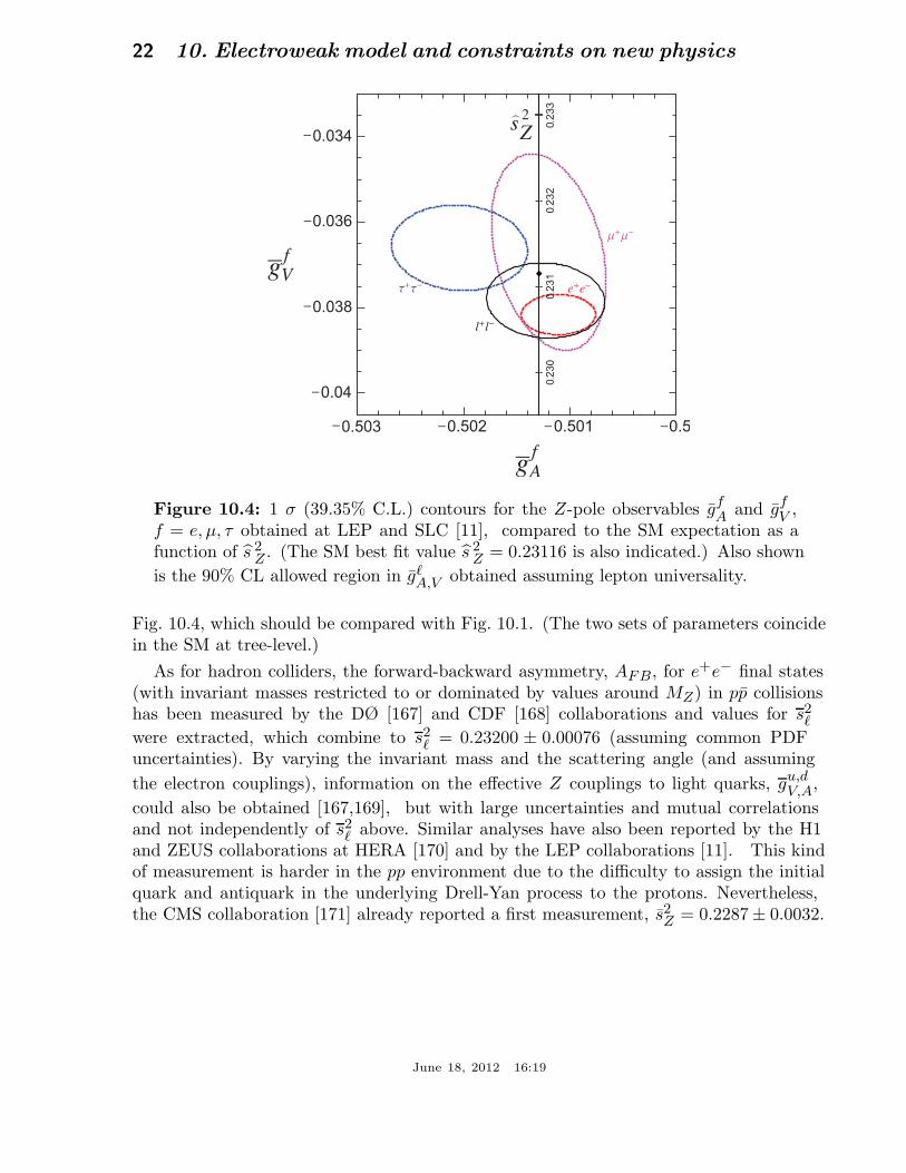
Figure 10.4: 1 σ (39.35% C.L.) contours for the Z-pole observables gfA and gf
V ,f = e, µ, τ obtained at LEP and SLC [11], compared to the SM expectation as afunction of s 2
Z . (The SM best fit value s 2Z = 0.23116 is also indicated.) Also shown
is the 90% CL allowed region in gℓA,V obtained assuming lepton universality.
Fig. 10.4, which should be compared with Fig. 10.1. (The two sets of parameters coincidein the SM at tree-level.)
As for hadron colliders, the forward-backward asymmetry, AFB, for e+e− final states(with invariant masses restricted to or dominated by values around MZ) in pp collisionshas been measured by the DØ [167] and CDF [168] collaborations and values for s2
ℓwere extracted, which combine to s2
ℓ = 0.23200 ± 0.00076 (assuming common PDFuncertainties). By varying the invariant mass and the scattering angle (and assuming
the electron couplings), information on the effective Z couplings to light quarks, gu,dV,A,
could also be obtained [167,169], but with large uncertainties and mutual correlationsand not independently of s2
ℓ above. Similar analyses have also been reported by the H1and ZEUS collaborations at HERA [170] and by the LEP collaborations [11]. This kindof measurement is harder in the pp environment due to the difficulty to assign the initialquark and antiquark in the underlying Drell-Yan process to the protons. Nevertheless,the CMS collaboration [171] already reported a first measurement, s2
Z = 0.2287± 0.0032.
June 18, 2012 16:19
10. Electroweak model and constraints on new physics 23
10.4.3. LEP 2 :
LEP 2 [172] ran at several energies above the Z pole up to ∼ 209 GeV. Measurementswere made of a number of observables, including the cross-sections for e+e− → f ffor f = q, µ−, τ−; the differential cross-sections for f = e−, µ−, τ−; Rq for q = b, c;AFB(f) for f = µ, τ, b, c; W branching ratios; and WW , WWγ, ZZ, single W , andsingle Z cross-sections. They are in good agreement with the SM predictions, with theexceptions of the total hadronic cross-section (1.7 σ high), Rb (2.1 σ low), and AFB(b)(1.6 σ low). Also, the negative result of the direct search for the SM Higgs boson excludedMH values below 114.4 GeV at the 95% CL [173]. This result is complementary to andcan be combined with [174] the limits inferred from the EW precision data.
The Z boson properties are extracted assuming the SM expressions for the γ–Zinterference terms. These have also been tested experimentally by performing moregeneral fits [172,175] to the LEP 1 and LEP 2 data. Assuming family universalitythis approach introduces three additional parameters relative to the standard fit [11],describing the γ–Z interference contribution to the total hadronic and leptoniccross-sections, jtot
had and jtotℓ , and to the leptonic forward-backward asymmetry, jfb
ℓ . E.g.,
jtothad ∼ gℓ
V ghadV = 0.277 ± 0.065, (10.41)
which is in agreement with the SM expectation [11] of 0.21 ± 0.01. These are valuabletests of the SM; but it should be cautioned that new physics is not expected to bedescribed by this set of parameters, since (i) they do not account for extra interactionsbeyond the standard weak neutral-current, and (ii) the photonic amplitude remains fixedto its SM value.
Strong constraints on anomalous triple and quartic gauge couplings have been obtainedat LEP 2 and the Tevatron as described in the Gauge & Higgs Bosons Particle Listings.
10.4.4. W and Z decays :
The partial decay width for gauge bosons to decay into massless fermions f1f2 (thenumerical values include the small EW radiative corrections and final state mass effects)is given by
Γ(W+ → e+νe) =GF M3
W
6√
2π≈ 226.36 ± 0.05 MeV , (10.42a)
Γ(W+ → uidj) =CGF M3
W
6√
2π|Vij |2 ≈ 706.34 ± 0.16 MeV |Vij |2, (10.42b)
Γ(Z → ψiψi) =CGF M3
Z
6√
2π
[gi2V + gi2
A
]≈
167.22 ± 0.01 MeV (νν),
84.00 ± 0.01 MeV (e+e−),
300.26 ± 0.05 MeV (uu),
383.04 ± 0.05 MeV (dd),
375.98 ∓ 0.03 MeV (bb).
(10.42c)
June 18, 2012 16:19
24 10. Electroweak model and constraints on new physics
For leptons C = 1, while for quarks
C = 3
[1 +
αs(MV )
π+ 1.409
α2s
π2− 12.77
α3s
π3− 80.0
α4s
π4
], (10.43)
where the 3 is due to color and the factor in brackets represents the universal part of theQCD corrections [176] for massless quarks [177]. The O(α4
s) contribution in Eq. (10.43)is recent [178]. The Z → f f widths contain a number of additional corrections: whichare different for vector and axial-vector partial widths and are included through orderα3
s and m4q(M
2Z) unless they are tiny; and singlet contributions starting from two-loop
order which are large, strongly top quark mass dependent, family universal, and flavornon-universal [181]. The QED factor 1 + 3αq2
f/4π, as well as two-loop order ααs and
α2 self-energy corrections [182] are also included. Working in the on-shell scheme, i.e.,expressing the widths in terms of GF M3
W,Z , incorporates the largest radiative corrections
from the running QED coupling [63,183]. EW corrections to the Z widths are thenincorporated by replacing g i2
V,A by g i2V,A. Hence, in the on-shell scheme the Z widths
are proportional to ρi ∼ 1 + ρt. The MS normalization accounts also for the leading EWcorrections [68]. There is additional (negative) quadratic mt dependence in the Z → bbvertex corrections [184] which causes Γ(bb) to decrease with mt. The dominant effect is
to multiply Γ(bb) by the vertex correction 1 + δρbb, where δρbb ∼ 10−2(− 12
m2t
M2Z
+ 15). In
practice, the corrections are included in ρb and κb, as discussed in Sec. 10.2.
For three fermion families the total widths are predicted to be
ΓZ ≈ 2.4960 ± 0.0002 GeV , ΓW ≈ 2.0915 ± 0.0005 GeV . (10.44)
We have assumed αs(MZ) = 0.1200. An uncertainty in αs of ±0.002 introduces anadditional uncertainty of 0.06% in the hadronic widths, corresponding to ±1 MeVin ΓZ . These predictions are to be compared with the experimental results, ΓZ =2.4952 ± 0.0023 GeV [11] and ΓW = 2.085 ± 0.042 GeV [185] (see the Gauge & HiggsBoson Particle Listings for more details).
10.5. Precision flavor physics
In addition to cross-sections, asymmetries, parity violation, W and Z decays, thereis a large number of experiments and observables testing the flavor structure of theSM. These are addressed elsewhere in this Review, and are generally not included inthis Section. However, we identify three precision observables with sensitivity to similartypes of new physics as the other processes discussed here. The branching fraction ofthe flavor changing transition b → sγ is of comparatively low precision, but since it is aloop-level process (in the SM) its sensitivity to new physics (and SM parameters, suchas heavy quark masses) is enhanced. A discussion can be found in earlier editions ofthis Review. The τ -lepton lifetime and leptonic branching ratios are primarily sensitiveto αs and not affected significantly by many types of new physics. However, having anindependent and reliable low energy measurement of αs in a global analysis allows the
June 18, 2012 16:19
10. Electroweak model and constraints on new physics 25
comparison with the Z lineshape determination of αs which shifts easily in the presenceof new physics contributions. By far the most precise observable discussed here is theanomalous magnetic moment of the muon (the electron magnetic moment is measured toeven greater precision and can be used to determine α, but its new physics sensitivity issuppressed by an additional factor of m2
e/m2µ). Its combined experimental and theoretical
uncertainty is comparable to typical new physics contributions.
The extraction of αs from the τ lifetime [186] is standing out from other determinationsbecause of a variety of independent reasons: (i) the τ -scale is low, so that uponextrapolation to the Z scale (where it can be compared to the theoretically cleanZ lineshape determinations) the αs error shrinks by about an order of magnitude;(ii) yet, this scale is high enough that perturbation theory and the operator productexpansion (OPE) can be applied; (iii) these observables are fully inclusive and thus freeof fragmentation and hadronization effects that would have to be modeled or measured;(iv) duality violation (DV) effects are most problematic near the branch cut but therethey are suppressed by a double zero at s = m2
τ ; (v) there are data [43] to constrainnon-perturbative effects both within (δD=6,8) and breaking (δDV ) the OPE; (vi) acomplete four-loop order QCD calculation is available [178]; (vii) large effects associatedwith the QCD β-function can be re-summed [187] in what has become known as contourimproved perturbation theory (CIPT). However, while there is no doubt that CIPT showsfaster convergence in the lower (calculable) orders, doubts have been cast on the methodby the observation that at least in a specific model [188], which includes the exactlyknown coefficients and theoretical constraints on the large-order behavior, ordinary fixedorder perturbation theory (FOPT) may nevertheless give a better approximation to thefull result. We therefore use the expressions [54,177,178,189],
ττ = ~1 − Bs
τ
Γeτ + Γµ
τ + Γudτ
= 291.13 ± 0.43 fs, (10.45)
Γudτ =
G2F m5
τ |Vud|264π3
S(mτ , MZ)
(1 +
3
5
m2τ − m2
µ
M2W
)×
[1 +αs(mτ )
π+ 5.202
α2s
π2+ 26.37
α3s
π3+ 127.1
α4s
π4+
α
π(85
24− π2
2) + δq], (10.46)
and Γeτ and Γ
µτ can be taken from Eq. (10.6) with obvious replacements. The relative
fraction of decays with ∆S = −1, Bsτ = 0.0286 ± 0.0007, is based on experimental
data since the value for the strange quark mass, ms(mτ ), is not well known andthe QCD expansion proportional to m2
s converges poorly and cannot be trusted.S(mτ , MZ) = 1.01907 ± 0.0003 is a logarithmically enhanced EW correction factor withhigher orders re-summed [190]. δq contains the dimension six and eight terms in theOPE, as well as DV effects, δD=6,8 + δDV = −0.004 ± 0.012 [191]. Depending on howδD=6, δD=8, and δDV are extracted, there are strong correlations not only between them,but also with the gluon condensate (D = 4) and possibly D > 8 terms. These latterare suppressed in Eq. (10.46) by additional factors of αs, but not so for more general
June 18, 2012 16:19
26 10. Electroweak model and constraints on new physics
weight functions. A simultaneous fit to all non-perturbative terms [191] (as is necessaryif one wants to avoid ad hoc assumptions) indicates that the αs errors may have beenunderestimated in the past. Higher statistics τ decay data [45] and spectral functions frome+e− annihilation (providing a larger fit window and thus more discriminatory powerand smaller correlations) are likely to reduce the δq error in the future. Also included inδq are quark mass effects and the D = 4 condensate contributions. An uncertainty ofsimilar size arises from the truncation of the FOPT series and is conservatively taken asthe α4
s term (this is re-calculated in each call of the fits, leading to an αs-dependent andthus asymmetric error) until a better understanding of the numerical differences betweenFOPT and CIPT has been gained. Our perturbative error covers almost the entire rangefrom using CIPT to assuming that the nearly geometric series in Eq. (10.46) continuesto higher orders. The experimental uncertainty in Eq. (10.45), is from the combinationof the two leptonic branching ratios with the direct ττ . Included are also various smalleruncertainties (±0.5 fs) from other sources which are dominated by the evolution fromthe Z scale. In total we obtain a ∼ 2% determination of αs(MZ) = 0.1193+0.0022
−0.0020, which
corresponds to αs(mτ ) = 0.327+0.019−0.016, and updates the result of Refs. 54 and 192. For
more details, see Refs. 191 and 193 where the τ spectral functions are used as additionalinput.
The world average of the muon anomalous magnetic moment‡,
aexpµ =
gµ − 2
2= (1165920.80± 0.63) × 10−9, (10.47)
is dominated by the final result of the E821 collaboration at BNL [194]. The QEDcontribution has been calculated to four loops [195] (fully analytically to threeloops [196,197]) , and the leading logarithms are included to five loops [198,199]. Theestimated SM EW contribution [200–202], aEW
µ = (1.52 ± 0.03) × 10−9, which includesleading two-loop [201] and three-loop [202] corrections, is at the level of twice the currentuncertainty.
The limiting factor in the interpretation of the result are the uncertainties fromthe two- and three-loop hadronic contribution. E.g., Ref. 20 obtained the valueahadµ = (69.23 ± 0.42) × 10−9 which combines CMD-2 [47] and SND [48] e+e− →
hadrons cross-section data with radiative return results from BaBar [50] and KLOE [51].This value suggests a 3.6 σ discrepancy between Eq. (10.47) and the SM prediction.An alternative analysis [20] using τ decay data and isospin symmetry (CVC) yields
‡ In what follows, we summarize the most important aspects of gµ − 2, and give somedetails about the evaluation in our fits. For more details see the dedicated contribution byA. Hocker and W. Marciano in this Review. There are some small numerical differences (atthe level of 0.1 standard deviation), which are well understood and mostly arise becauseinternal consistency of the fits requires the calculation of all observables from analyticalexpressions and common inputs and fit parameters, so that an independent evaluation isnecessary for this Section. Note, that in the spirit of a global analysis based on all availableinformation we have chosen here to average in the τ decay data, as well.
June 18, 2012 16:19
10. Electroweak model and constraints on new physics 27
ahadµ = (70.15±0.47)×10−9. This result implies a smaller conflict (2.4 σ) with Eq. (10.47).
Thus, there is also a discrepancy between the spectral functions obtained from the twomethods. For example, if one uses the e+e− data and CVC to predict the branching ratiofor τ− → ντπ−π0 decays [20] we obtain an average of BCVC = 24.93 ± 0.13 ± 0.22CVC,while the average of the directly measured branching ratio yields 25.51 ± 0.09, whichis 2.3 σ higher. It is important to understand the origin of this difference, but twoobservations point to the conclusion that at least some of it is experimental: (i) Thereis also a direct discrepancy of 1.9 σ between BCVC derived from BaBar (which is notinconsistent with τ decays) and KLOE. (ii) Isospin violating corrections have beenstudied in detail in Ref. 203 and found to be largely under control. The largest effect isdue to higher-order EW corrections [204] but introduces a negligible uncertainty [190].Nevertheless, ahad
µ is often evaluated excluding the τ decay data arguing [205] that CVC
breaking effects (e.g., through a relatively large mass difference between the ρ± and ρ0
vector mesons) may be larger than expected. (This may also be relevant [205] in thecontext of the NuTeV result discussed above.) Experimentally [45], this mass difference isindeed larger than expected, but then one would also expect a significant width differencewhich is contrary to observation [45]. Fortunately, due to the suppression at large s(from where the conflicts originate) these problems are less pronounced as far as ahad
µ isconcerned. In the following we view all differences in spectral functions as (systematic)fluctuations and average the results.
An additional uncertainty is induced by the hadronic three-loop light-by-lightscattering contribution. Two recent and inherently different model calculations yieldaLBLSµ = (+1.36 ± 0.25) × 10−9 [206] and aLBLS
µ = +1.37+0.15−0.27 × 10⁻⁹ [207] which are
higher than previous evaluations [208,209]. The sign of this effect is opposite [208] tothe one quoted in the 2002 edition of this Review, and has subsequently been confirmedby two other groups [209]. There is also the upper bound aLBLS
µ < 1.59 × 10⁻⁹ [207]but this requires an ad hoc assumption, too. The recent Ref. 210 quotes the valueaLBLSµ = (+1.05 ± 0.26) × 10−9, which we shift by 2 × 10⁻¹¹ to account for the more
accurate charm quark treatment of Ref. 207. We also increase the error to cover allevaluations, and we will use aLBLS
µ = (+1.07 ± 0.32) × 10−9 in the fits.
Other hadronic effects at three-loop order contribute [211] ahadµ (α3) = (−1.00 ±
0.06) × 10−9. Correlations with the two-loop hadronic contribution and with ∆α(MZ)(see Sec. 10.2) were considered in Ref. 197 which also contains analytic results for theperturbative QCD contribution.
Altogether, the SM prediction is
atheoryµ = (1165918.41± 0.48) × 10−9 , (10.48)
where the error is from the hadronic uncertainties excluding parametric ones such asfrom αs and the heavy quark masses. Using a correlation of about 84% from the datainput to the vacuum polarization integrals [20], we estimate the correlation of the total(experimental plus theoretical) uncertainty in aµ with ∆α(MZ) as 24%. The overall3.0 σ discrepancy between the experimental and theoretical aµ values could be due tofluctuations (the E821 result is statistics dominated) or underestimates of the theoretical
June 18, 2012 16:19
28 10. Electroweak model and constraints on new physics
uncertainties. On the other hand, gµ − 2 is also affected by many types of new physics,such as supersymmetric models with large tan β and moderately light superparticlemasses [212]. Thus, the deviation could also arise from physics beyond the SM.
10.6. Global fit results
In this section we present the results of global fits to the experimental data discussedin Sec. 10.3–Sec. 10.5. For earlier analyses see Refs. 128 and 213.
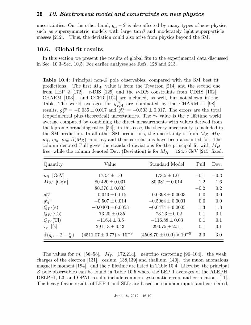
Table 10.4: Principal non-Z pole observables, compared with the SM best fitpredictions. The first MW value is from the Tevatron [214] and the second onefrom LEP 2 [172]. e-DIS [129] and the ν-DIS constraints from CDHS [102],CHARM [103], and CCFR [104] are included, as well, but not shown in theTable. The world averages for gνe
V,A are dominated by the CHARM II [98]
results, gνeV = −0.035 ± 0.017 and gνe
A = −0.503 ± 0.017. The errors are the total(experimental plus theoretical) uncertainties. The ττ value is the τ lifetime worldaverage computed by combining the direct measurements with values derived fromthe leptonic branching ratios [54]; in this case, the theory uncertainty is included inthe SM prediction. In all other SM predictions, the uncertainty is from MZ , MH ,mt, mb, mc, α(MZ), and αs, and their correlations have been accounted for. Thecolumn denoted Pull gives the standard deviations for the principal fit with MH
free, while the column denoted Dev. (Deviation) is for MH = 124.5 GeV [215] fixed.
Quantity Value Standard Model Pull Dev.
mt [GeV] 173.4 ± 1.0 173.5 ± 1.0 −0.1 −0.3
MW [GeV] 80.420 ± 0.031 80.381 ± 0.014 1.2 1.6
80.376 ± 0.033 −0.2 0.2
gνeV −0.040 ± 0.015 −0.0398 ± 0.0003 0.0 0.0
gνeA −0.507 ± 0.014 −0.5064 ± 0.0001 0.0 0.0
QW (e) −0.0403 ± 0.0053 −0.0474 ± 0.0005 1.3 1.3
QW (Cs) −73.20 ± 0.35 −73.23 ± 0.02 0.1 0.1
QW (Tl) −116.4 ± 3.6 −116.88 ± 0.03 0.1 0.1
ττ [fs] 291.13 ± 0.43 290.75 ± 2.51 0.1 0.1
12 (gµ − 2 − α
π ) (4511.07 ± 0.77) × 10−9 (4508.70 ± 0.09) × 10−9 3.0 3.0
The values for mt [56–58], MW [172,214], neutrino scattering [96–104], the weakcharges of the electron [131], cesium [138,139] and thallium [140], the muon anomalousmagnetic moment [194], and the τ lifetime are listed in Table 10.4. Likewise, the principalZ pole observables can be found in Table 10.5 where the LEP 1 averages of the ALEPH,DELPHI, L3, and OPAL results include common systematic errors and correlations [11].The heavy flavor results of LEP 1 and SLD are based on common inputs and correlated,
June 18, 2012 16:19
10. Electroweak model and constraints on new physics 29
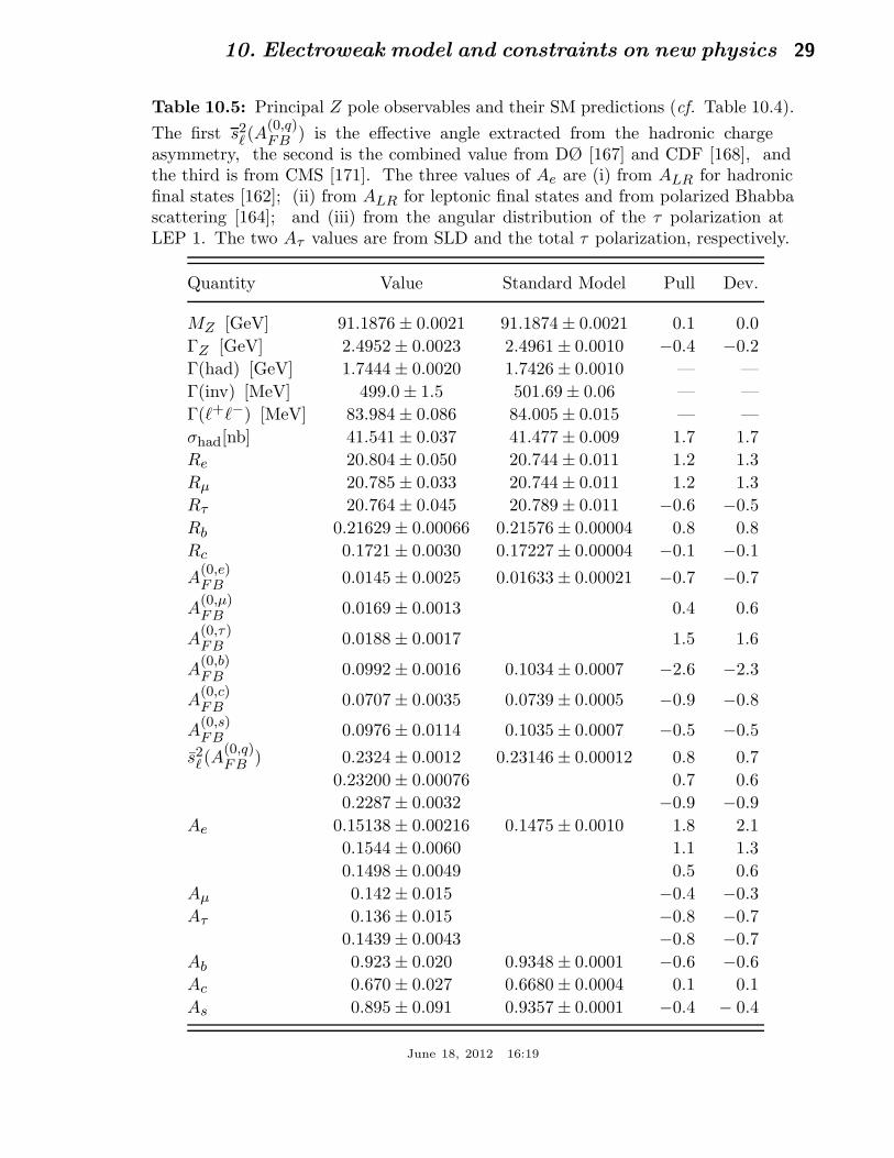
Table 10.5: Principal Z pole observables and their SM predictions (cf. Table 10.4).
The first s2ℓ (A
(0,q)FB ) is the effective angle extracted from the hadronic charge
asymmetry, the second is the combined value from DØ [167] and CDF [168], andthe third is from CMS [171]. The three values of Ae are (i) from ALR for hadronicfinal states [162]; (ii) from ALR for leptonic final states and from polarized Bhabbascattering [164]; and (iii) from the angular distribution of the τ polarization atLEP 1. The two Aτ values are from SLD and the total τ polarization, respectively.
Quantity Value Standard Model Pull Dev.
MZ [GeV] 91.1876 ± 0.0021 91.1874 ± 0.0021 0.1 0.0
ΓZ [GeV] 2.4952 ± 0.0023 2.4961 ± 0.0010 −0.4 −0.2
Γ(had) [GeV] 1.7444 ± 0.0020 1.7426 ± 0.0010 — —
Γ(inv) [MeV] 499.0 ± 1.5 501.69± 0.06 — —
Γ(ℓ+ℓ−) [MeV] 83.984 ± 0.086 84.005 ± 0.015 — —
σhad[nb] 41.541 ± 0.037 41.477 ± 0.009 1.7 1.7
Re 20.804 ± 0.050 20.744 ± 0.011 1.2 1.3
Rµ 20.785 ± 0.033 20.744 ± 0.011 1.2 1.3
Rτ 20.764 ± 0.045 20.789 ± 0.011 −0.6 −0.5
Rb 0.21629 ± 0.00066 0.21576 ± 0.00004 0.8 0.8
Rc 0.1721 ± 0.0030 0.17227 ± 0.00004 −0.1 −0.1
A(0,e)FB 0.0145 ± 0.0025 0.01633 ± 0.00021 −0.7 −0.7
A(0,µ)FB 0.0169 ± 0.0013 0.4 0.6
A(0,τ)FB 0.0188 ± 0.0017 1.5 1.6
A(0,b)FB 0.0992 ± 0.0016 0.1034 ± 0.0007 −2.6 −2.3
A(0,c)FB 0.0707 ± 0.0035 0.0739 ± 0.0005 −0.9 −0.8
A(0,s)FB 0.0976 ± 0.0114 0.1035 ± 0.0007 −0.5 −0.5
s2ℓ (A
(0,q)FB ) 0.2324 ± 0.0012 0.23146 ± 0.00012 0.8 0.7
0.23200 ± 0.00076 0.7 0.6
0.2287 ± 0.0032 −0.9 −0.9
Ae 0.15138 ± 0.00216 0.1475 ± 0.0010 1.8 2.1
0.1544 ± 0.0060 1.1 1.3
0.1498 ± 0.0049 0.5 0.6
Aµ 0.142 ± 0.015 −0.4 −0.3
Aτ 0.136 ± 0.015 −0.8 −0.7
0.1439 ± 0.0043 −0.8 −0.7
Ab 0.923 ± 0.020 0.9348 ± 0.0001 −0.6 −0.6
Ac 0.670 ± 0.027 0.6680 ± 0.0004 0.1 0.1
As 0.895 ± 0.091 0.9357 ± 0.0001 −0.4 − 0.4
June 18, 2012 16:19
30 10. Electroweak model and constraints on new physics
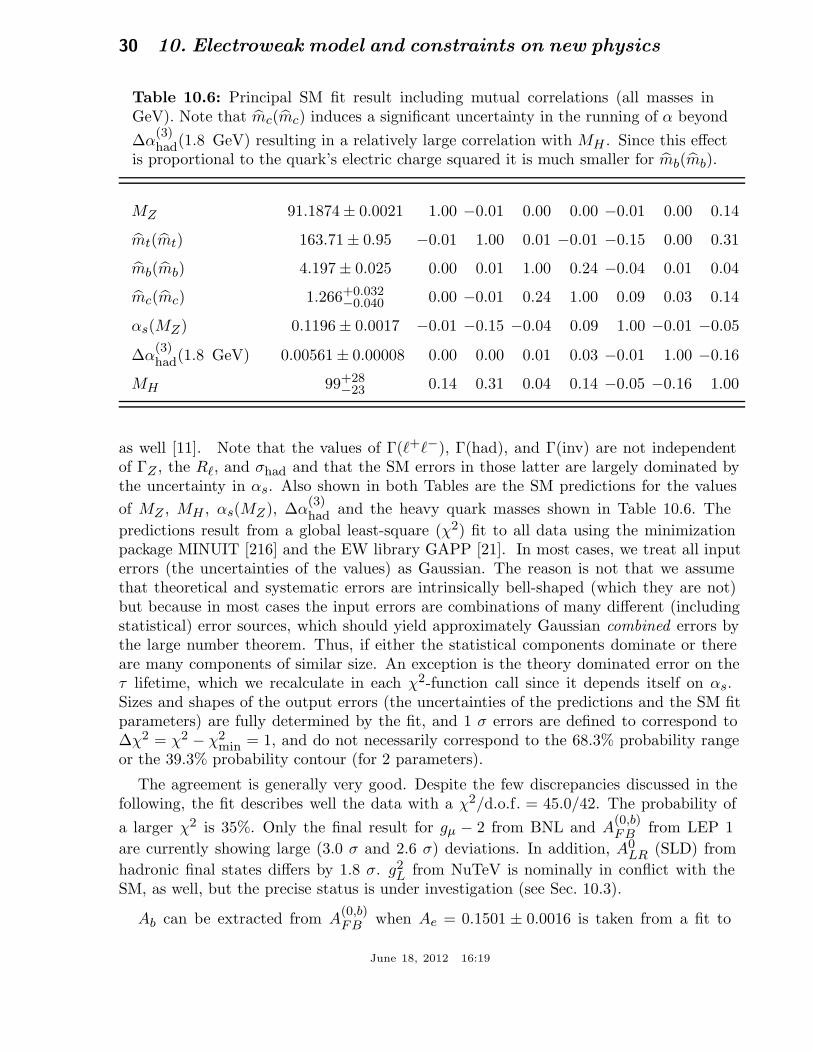
Table 10.6: Principal SM fit result including mutual correlations (all masses inGeV). Note that mc(mc) induces a significant uncertainty in the running of α beyond
∆α(3)had(1.8 GeV) resulting in a relatively large correlation with MH . Since this effect
is proportional to the quark’s electric charge squared it is much smaller for mb(mb).
MZ 91.1874 ± 0.0021 1.00 −0.01 0.00 0.00 −0.01 0.00 0.14
mt(mt) 163.71 ± 0.95 −0.01 1.00 0.01 −0.01 −0.15 0.00 0.31
mb(mb) 4.197 ± 0.025 0.00 0.01 1.00 0.24 −0.04 0.01 0.04
mc(mc) 1.266+0.032−0.040 0.00 −0.01 0.24 1.00 0.09 0.03 0.14
αs(MZ) 0.1196 ± 0.0017 −0.01 −0.15 −0.04 0.09 1.00 −0.01 −0.05
∆α(3)had(1.8 GeV) 0.00561 ± 0.00008 0.00 0.00 0.01 0.03 −0.01 1.00 −0.16
MH 99+28−23 0.14 0.31 0.04 0.14 −0.05 −0.16 1.00
as well [11]. Note that the values of Γ(ℓ+ℓ−), Γ(had), and Γ(inv) are not independentof ΓZ , the Rℓ, and σhad and that the SM errors in those latter are largely dominated bythe uncertainty in αs. Also shown in both Tables are the SM predictions for the values
of MZ , MH , αs(MZ), ∆α(3)had and the heavy quark masses shown in Table 10.6. The
predictions result from a global least-square (χ2) fit to all data using the minimizationpackage MINUIT [216] and the EW library GAPP [21]. In most cases, we treat all inputerrors (the uncertainties of the values) as Gaussian. The reason is not that we assumethat theoretical and systematic errors are intrinsically bell-shaped (which they are not)but because in most cases the input errors are combinations of many different (includingstatistical) error sources, which should yield approximately Gaussian combined errors bythe large number theorem. Thus, if either the statistical components dominate or thereare many components of similar size. An exception is the theory dominated error on theτ lifetime, which we recalculate in each χ2-function call since it depends itself on αs.Sizes and shapes of the output errors (the uncertainties of the predictions and the SM fitparameters) are fully determined by the fit, and 1 σ errors are defined to correspond to∆χ2 = χ2 − χ2
min = 1, and do not necessarily correspond to the 68.3% probability rangeor the 39.3% probability contour (for 2 parameters).
The agreement is generally very good. Despite the few discrepancies discussed in thefollowing, the fit describes well the data with a χ2/d.o.f. = 45.0/42. The probability of
a larger χ2 is 35%. Only the final result for gµ − 2 from BNL and A(0,b)FB from LEP 1
are currently showing large (3.0 σ and 2.6 σ) deviations. In addition, A0LR (SLD) from
hadronic final states differs by 1.8 σ. g2L from NuTeV is nominally in conflict with the
SM, as well, but the precise status is under investigation (see Sec. 10.3).
Ab can be extracted from A(0,b)FB when Ae = 0.1501 ± 0.0016 is taken from a fit to
June 18, 2012 16:19
10. Electroweak model and constraints on new physics 31
leptonic asymmetries (using lepton universality). The result, Ab = 0.881 ± 0.017, is 3.2 σ
below the SM prediction§ and also 1.6 σ below Ab = 0.923± 0.020 obtained from AFBLR (b)
at SLD. Thus, it appears that at least some of the problem in A(0,b)FB is experimental.
Note, however, that the uncertainty in A(0,b)FB is strongly statistics dominated. The
combined value, Ab = 0.899± 0.013 deviates by 2.8 σ. It would be difficult to account forthis 4.0% deviation by new physics that enters only at the level of radiative correctionssince about a 20% correction to κb would be necessary to account for the central valueof Ab [217]. If this deviation is due to new physics, it is most likely of tree-level typeaffecting preferentially the third generation. Examples include the decay of a scalarneutrino resonance [218], mixing of the b quark with heavy exotics [219], and a heavy Z ′
with family-nonuniversal couplings [220,221]. It is difficult, however, to simultaneouslyaccount for Rb, which has been measured on the Z peak and off-peak [222] at LEP 1.An average of Rb measurements at LEP 2 at energies between 133 and 207 GeV is 2.1 σ
below the SM prediction, while A(b)FB (LEP 2) is 1.6 σ low [172].
The left-right asymmetry, A0LR = 0.15138 ± 0.00216 [162], based on all hadronic data
from 1992–1998 differs 1.8 σ from the SM expectation of 0.1475 ± 0.0010. The combinedvalue of Aℓ = 0.1513 ± 0.0021 from SLD (using lepton-family universality and includingcorrelations) is also 1.8 σ above the SM prediction; but there is experimental agreementbetween this SLD value and the LEP 1 value, Aℓ = 0.1481 ± 0.0027, obtained from a fit
to A(0,ℓ)FB , Ae(Pτ ), and Aτ (Pτ ), again assuming universality.
The observables in Table 10.4 and Table 10.5, as well as some other less preciseobservables, are used in the global fits described below. In all fits, the errors includefull statistical, systematic, and theoretical uncertainties. The correlations on the LEP 1lineshape and τ polarization, the LEP/SLD heavy flavor observables, the SLD leptonasymmetries, and the deep inelastic and ν-e scattering observables, are included. The
theoretical correlations between ∆α(5)had and gµ − 2, and between the charm and bottom
quark masses, are also accounted for.
The data allow a simultaneous determination of MZ , MH , mt, and the strong coupling
αs(MZ). (mc, mb, and ∆α(3)had are also allowed to float in the fits, subject to the
theoretical constraints [19,54] described in Sec. 10.2. These are correlated with αs.) αs
is determined mainly from Rℓ, ΓZ , σhad, and ττ and is only weakly correlated withthe other variables. The global fit to all data, including the hadron collider averagemt = 173.4 ± 1.0 GeV, yields the result in Table 10.6 (the MS top quark mass given therecorresponds to mt = 173.5 ± 1.0 GeV). The weak mixing angle is determined to
s 2Z = 0.23116 ± 0.00012, s2
W = 0.22296± 0.00028,
while the corresponding effective angle is related by Eq. (10.18), i.e., s2ℓ = 0.23146 ±
0.00012.
§ Alternatively, one can use Aℓ = 0.1481 ± 0.0027, which is from LEP 1 alone and inexcellent agreement with the SM, and obtain Ab = 0.893± 0.022 which is 1.9 σ low. Thisillustrates that some of the discrepancy is related to the one in ALR.
June 18, 2012 16:19
32 10. Electroweak model and constraints on new physics
As described in Sec. 10.2 and the paragraph following Eq. (10.47) in Sec. 10.5, thereis considerable stress in the experimental e+e− spectral functions and also conflict whenthese are compared with τ decay spectral functions. These are below or above the 2σlevel (depending on what is actually compared) but not larger than the deviations ofsome other quantities entering our analyses. The number and size or these deviationsare not inconsistent with what one would expect to happen as a result of randomfluctuations. It is nevertheless instructive to study the effect of doubling the uncertainty
in ∆α(3)had(1.8 GeV) = (55.50± 0.78)× 10−4, (see Sec. 10.2) on the extracted Higgs mass.
The result, MH = 95+28−23 GeV, demonstrates that the uncertainty in ∆αhad is currently
of only secondary importance. Note also, that a shift of ±0.0001 in ∆α(3)had(1.8 GeV)
corresponds to a shift of ∓5 GeV in MH or about one fifth of its total uncertainty.The hadronic contribution to α(MZ) is correlated with gµ − 2 (see Sec. 10.5). Themeasurement of the latter is higher than the SM prediction, and its inclusion in the fitfavors a larger α(MZ) and a lower MH (currently by about 4 GeV).
The weak mixing angle can be determined from Z pole observables, MW , and froma variety of neutral-current processes spanning a very wide Q2 range. The results (forthe older low energy neutral-current data see Refs. 128 and 213) shown in Table 10.7are in reasonable agreement with each other, indicating the quantitative success of theSM. The largest discrepancy is the value s 2
Z = 0.23193 ± 0.00028 from the forward-backward asymmetries into bottom and charm quarks, which is 2.8 σ above the value0.23116 ± 0.00012 from the global fit to all data. Similarly, s 2
Z = 0.23067 ± 0.00029from the SLD asymmetries (in both cases when combined with MZ) is 1.8 σ low.The SLD result has the additional difficulty (within the SM) of implying very low andexcluded [173] Higgs masses. This is also true for s 2
Z = 0.23098 ± 0.00022 from MWand MZ and — as a consequence — for the global fit. We have therefore included inTable 10.4 and Table 10.5 an additional column (denoted Deviation) indicating thedeviations if MH = 124.5 GeV [215] is fixed.
The extracted Z pole value of αs(MZ) is based on a formula with negligible theoreticaluncertainty if one assumes the exact validity of the SM. One should keep in mind,however, that this value, αs(MZ) = 0.1197 ± 0.0028, is very sensitive to such typesof new physics as non-universal vertex corrections. In contrast, the value derived fromτ decays, αs(MZ) = 0.1193+0.0022
−0.0020, is theory dominated but less sensitive to new physics.The two values are in remarkable agreement with each other. They are also in perfectagreement with the averages from jet-event shapes in e+e− annihilation (0.1172± 0.0037)and lattice simulations (0.1185 ± 0.0007), whereas the DIS average (0.1150 ± 0.0021) issomewhat lower. For more details, other determinations, and references, see our Section 9on “Quantum Chromodynamics” in this Review.
Using α(MZ) and s 2Z as inputs, one can predict αs(MZ) assuming grand unification.
One predicts [223] αs(MZ) = 0.130 ± 0.001 ± 0.01 for the simplest theories based on theminimal supersymmetric extension of the SM, where the first (second) uncertainty isfrom the inputs (thresholds). This is slightly larger, but consistent with the experimentalαs(MZ) = 0.1196 ± 0.0017 from the Z lineshape and the τ lifetime, as well as withmost other determinations. Non-supersymmetric unified theories predict the low value
June 18, 2012 16:19
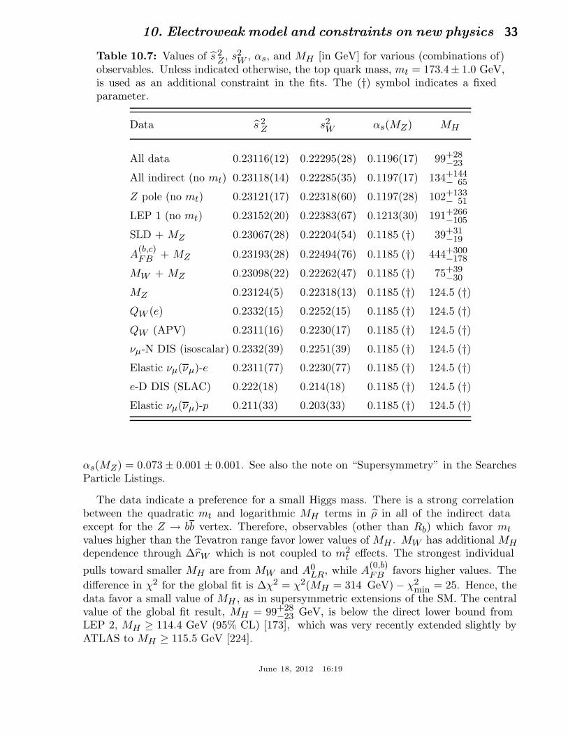
10. Electroweak model and constraints on new physics 33
Table 10.7: Values of s 2Z , s2
W , αs, and MH [in GeV] for various (combinations of)observables. Unless indicated otherwise, the top quark mass, mt = 173.4± 1.0 GeV,is used as an additional constraint in the fits. The (†) symbol indicates a fixedparameter.
Data s 2Z s2
W αs(MZ) MH
All data 0.23116(12) 0.22295(28) 0.1196(17) 99+28−23
All indirect (no mt) 0.23118(14) 0.22285(35) 0.1197(17) 134+144− 65
Z pole (no mt) 0.23121(17) 0.22318(60) 0.1197(28) 102+133− 51
LEP 1 (no mt) 0.23152(20) 0.22383(67) 0.1213(30) 191+266−105
SLD + MZ 0.23067(28) 0.22204(54) 0.1185 (†) 39+31−19
A(b,c)FB + MZ 0.23193(28) 0.22494(76) 0.1185 (†) 444+300
−178
MW + MZ 0.23098(22) 0.22262(47) 0.1185 (†) 75+39−30
MZ 0.23124(5) 0.22318(13) 0.1185 (†) 124.5 (†)QW (e) 0.2332(15) 0.2252(15) 0.1185 (†) 124.5 (†)QW (APV) 0.2311(16) 0.2230(17) 0.1185 (†) 124.5 (†)νµ-N DIS (isoscalar) 0.2332(39) 0.2251(39) 0.1185 (†) 124.5 (†)Elastic νµ(νµ)-e 0.2311(77) 0.2230(77) 0.1185 (†) 124.5 (†)e-D DIS (SLAC) 0.222(18) 0.214(18) 0.1185 (†) 124.5 (†)Elastic νµ(νµ)-p 0.211(33) 0.203(33) 0.1185 (†) 124.5 (†)
αs(MZ) = 0.073 ± 0.001 ± 0.001. See also the note on “Supersymmetry” in the SearchesParticle Listings.
The data indicate a preference for a small Higgs mass. There is a strong correlationbetween the quadratic mt and logarithmic MH terms in ρ in all of the indirect dataexcept for the Z → bb vertex. Therefore, observables (other than Rb) which favor mt
values higher than the Tevatron range favor lower values of MH . MW has additional MHdependence through ∆rW which is not coupled to m2
t effects. The strongest individual
pulls toward smaller MH are from MW and A0LR, while A
(0,b)FB favors higher values. The
difference in χ2 for the global fit is ∆χ2 = χ2(MH = 314 GeV) − χ2min = 25. Hence, the
data favor a small value of MH , as in supersymmetric extensions of the SM. The centralvalue of the global fit result, MH = 99+28
−23 GeV, is below the direct lower bound fromLEP 2, MH ≥ 114.4 GeV (95% CL) [173], which was very recently extended slightly byATLAS to MH ≥ 115.5 GeV [224].
June 18, 2012 16:19

34 10. Electroweak model and constraints on new physics
Figure 10.5: One-standard-deviation (39.35%) uncertainties in MH as a functionof mt for various inputs, and the 90% CL region (∆χ2 = 4.605) allowed by all data.αs(MZ) = 0.1185 is assumed except for the fits including the Z lineshape or lowenergy data. The bright (yellow) bands are excluded by one experiment and theremaining (gray) regions are ruled out by more than one experiment (95% CL).
The 90% central confidence range from all precision data is
68 GeV ≤ MH ≤ 155 GeV. (10.49)
Including the results of the direct searches at LEP 2 [173] and the Tevatron [225] as extracontributions to the likelihood function reduces the 95% upper limit to MH ≤ 150 GeV.As two further refinements, we account for (i) theoretical uncertainties from uncalculatedhigher order contributions by allowing the T parameter (see next subsection) subject tothe constraint T = 0 ± 0.02, (ii) the MH dependence of the correlation matrix whichgives slightly more weight to lower Higgs masses [226]. The resulting limits at 95 (90,99)% CL are, respectively,
MH ≤ 175 (148, 210) GeV. (10.50)
In their Higgs searches in pp collisions with CM energy of 7 TeV, both ATLAS [224]and CMS [227] find results consistent with Eq. (10.50) and currently report & 2 σexcess fluctuation near MH = 119.5 GeV (CMS only), MH = 124 GeV (CMS), andMH = 126 GeV (ATLAS only). Of course, these excesses do not constitute a discovery.However, it is useful to take them at face value for comparison with the precision data inTable 10.4, Table 10.5, and Table 10.7. A combination of all available data yields (at the68% CL) [215]
MH = 124.5 ± 0.8 GeV. (10.51)
June 18, 2012 16:19

10. Electroweak model and constraints on new physics 35
Figure 10.6: One-standard-deviation (39.35%) region in MW as a function of mt
for the direct and indirect precision data, and the 90% CL region (∆χ2 = 4.605)allowed by all precision data. The SM predictions are also indicated, where theblue bands for Higgs masses between 115.5 and 127 GeV and beyond 600 GeVare currently allowed at the 95% CL. The bright (yellow) bands are excluded byone experiment and the remaining (gray) regions are ruled out by more than oneexperiment (95% CL).
The resulting probability distribution has a twin peak structure (besides a smallermaximum at MH = 118.5 GeV) with almost equal probability at MH = 124 GeV andMH = 125 GeV [215].
One can also carry out a fit to the indirect data alone, i.e., without including theconstraint, mt = 173.4 ± 1.0 GeV, from the hadron colliders. (The indirect predictionis for the MS mass, mt(mt) = 167.5+8.9
−7.3 GeV, which is in the end converted to the
pole mass). One obtains mt = 177.5+9.4−7.8 GeV, in perfect agreement with the direct
Tevatron/LHC average. Using this indirect top mass value, the tendency for a light Higgspersists and Eq. (10.49) becomes 46 GeV ≤ MH ≤ 306 GeV. The relations between MHand mt for various observables are shown in Fig. 10.5.
One can also determine the radiative correction parameters ∆r: from the global fit oneobtains ∆r = 0.0352±0.0009 and ∆rW = 0.06945±0.00019. MW measurements [172,214](when combined with MZ) are equivalent to measurements of ∆r = 0.0342 ± 0.0015,which is 0.9 σ below the result from all other data, ∆r = 0.0358 ± 0.0011. Fig. 10.6shows the 1 σ contours in the MW -mt plane from the direct and indirect determinations,as well as the combined 90% CL region. The indirect determination uses MZ fromLEP 1 as input, which is defined assuming an s-dependent decay width. MW then
June 18, 2012 16:19
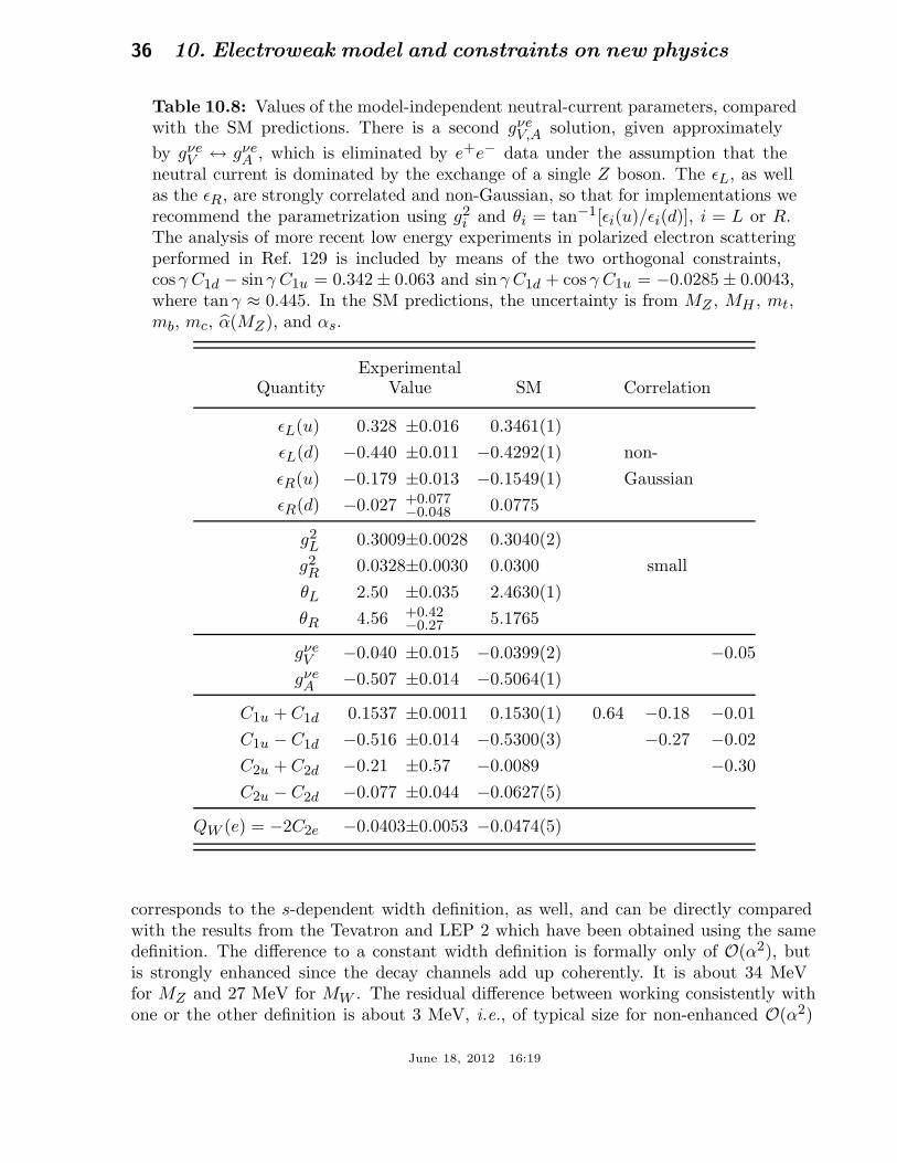
36 10. Electroweak model and constraints on new physics
Table 10.8: Values of the model-independent neutral-current parameters, comparedwith the SM predictions. There is a second gνe
V,A solution, given approximately
by gνeV ↔ gνe
A , which is eliminated by e+e− data under the assumption that theneutral current is dominated by the exchange of a single Z boson. The ǫL, as wellas the ǫR, are strongly correlated and non-Gaussian, so that for implementations werecommend the parametrization using g2
i and θi = tan−1[ǫi(u)/ǫi(d)], i = L or R.The analysis of more recent low energy experiments in polarized electron scatteringperformed in Ref. 129 is included by means of the two orthogonal constraints,cos γ C1d − sin γ C1u = 0.342 ± 0.063 and sin γ C1d + cos γ C1u = −0.0285 ± 0.0043,where tan γ ≈ 0.445. In the SM predictions, the uncertainty is from MZ , MH , mt,mb, mc, α(MZ), and αs.
ExperimentalQuantity Value SM Correlation
ǫL(u) 0.328 ±0.016 0.3461(1)
ǫL(d) −0.440 ±0.011 −0.4292(1) non-
ǫR(u) −0.179 ±0.013 −0.1549(1) Gaussian
ǫR(d) −0.027 +0.077−0.048 0.0775
g2L 0.3009±0.0028 0.3040(2)
g2R 0.0328±0.0030 0.0300 small
θL 2.50 ±0.035 2.4630(1)
θR 4.56 +0.42−0.27 5.1765
gνeV −0.040 ±0.015 −0.0399(2) −0.05
gνeA −0.507 ±0.014 −0.5064(1)
C1u + C1d 0.1537 ±0.0011 0.1530(1) 0.64 −0.18 −0.01
C1u − C1d −0.516 ±0.014 −0.5300(3) −0.27 −0.02
C2u + C2d −0.21 ±0.57 −0.0089 −0.30
C2u − C2d −0.077 ±0.044 −0.0627(5)
QW (e) = −2C2e −0.0403±0.0053 −0.0474(5)
corresponds to the s-dependent width definition, as well, and can be directly comparedwith the results from the Tevatron and LEP 2 which have been obtained using the samedefinition. The difference to a constant width definition is formally only of O(α2), butis strongly enhanced since the decay channels add up coherently. It is about 34 MeVfor MZ and 27 MeV for MW . The residual difference between working consistently withone or the other definition is about 3 MeV, i.e., of typical size for non-enhanced O(α2)
June 18, 2012 16:19
10. Electroweak model and constraints on new physics 37
corrections [74–77].
Most of the parameters relevant to ν-hadron, ν-e, e-hadron, and e−e± processes aredetermined uniquely and precisely from the data in “model-independent” fits (i.e., fitswhich allow for an arbitrary EW gauge theory). The values for the parameters defined inEqs. (10.19)–(10.22) are given in Table 10.8 along with the predictions of the SM. Theagreement is very good. (The ν-hadron results including the original NuTeV data canbe found in the 2006 edition of this Review, and fits with modified NuTeV constraintsin the 2008 and 2010 editions.) The off Z pole e+e− results are difficult to present ina model-independent way because Z propagator effects are non-negligible at TRISTAN,PETRA, PEP, and LEP 2 energies. However, assuming e-µ-τ universality, the low energylepton asymmetries imply [159] 4 (ge
A)2 = 0.99 ± 0.05, in good agreement with the SMprediction ≃ 1.
10.7. Constraints on new physics
The Z pole, W mass, and low energy data can be used to search for and set limits ondeviations from the SM. We will mainly discuss the effects of exotic particles (with heavymasses Mnew ≫ MZ in an expansion in MZ/Mnew) on the gauge boson self-energies.(Brief remarks are made on new physics which is not of this type.) Most of the effectson precision measurements can be described by three gauge self-energy parameters S, T ,and U . We will define these, as well as related parameters, such as ρ0, ǫi, and ǫi, to arisefrom new physics only. I.e., they are equal to zero (ρ0 = 1) exactly in the SM, and do notinclude any (loop induced) contributions that depend on mt or MH , which are treatedseparately. Our treatment differs from most of the original papers.
Many extensions of the SM can be described by the ρ0 parameter,
ρ0 ≡ M2W
M2Z c 2
Z ρ, (10.52)
which describes new sources of SU(2) breaking that cannot be accounted for by the SMHiggs doublet or mt effects. ρ is calculated as in Eq. (10.13) assuming the validity ofthe SM. In the presence of ρ0 6= 1, Eq. (10.52) generalizes the second Eq. (10.13) whilethe first remains unchanged. Provided that the new physics which yields ρ0 6= 1 is asmall perturbation which does not significantly affect the radiative corrections, ρ0 can beregarded as a phenomenological parameter which multiplies GF in Eqs. (10.19)–(10.22),(10.36), and ΓZ in Eq. (10.42c). There are enough data to determine ρ0, MH , mt, andαs, simultaneously. From the global fit,
ρ0 = 1.0004+0.0003−0.0004 , (10.53)
115.5 GeV ≤ MH ≤ 127 GeV, (10.54)
mt = 173.4 ± 1.0 GeV, (10.55)
αs(MZ) = 0.1195 ± 0.0017, (10.56)
June 18, 2012 16:19

38 10. Electroweak model and constraints on new physics
where the limits on MH are nominal direct search bounds at the 95% CL [173,224,227].In addition, the LHC is not yet sensitive to very large values of MH > 600 GeV whichare thus not ruled out either. In this very high mass scenario, we obtain,
ρ0 = 1.0024+0.0010−0.0003 , (10.57)
0.6 TeV ≤ MH ≤ 1.2 TeV, (10.58)
αs(MZ) = 0.1191± 0.0016, (10.59)
with the same mt. Finally, if the direct search results are ignored entirely one findsMH = 189+568
−114 GeV and ρ0 = 1.0008+0.0020−0.0011. The result in Eq. (10.53) is slightly
above but consistent with the SM expectation, ρ0 = 1. It can be used to constrainhigher-dimensional Higgs representations to have vacuum expectation values of less thana few percent of those of the doublets. Indeed, the relation between MW and MZ ismodified if there are Higgs multiplets with weak isospin > 1/2 with significant vacuumexpectation values. For a general (charge-conserving) Higgs structure,
ρ0 =
∑i[t(i)(t(i) + 1) − t3(i)
2]|vi|22
∑i t3(i)2|vi|2
, (10.60)
where vi is the expectation value of the neutral component of a Higgs multiplet withweak isospin t(i) and third component t3(i). In order to calculate to higher orders insuch theories one must define a set of four fundamental renormalized parameters whichone may conveniently choose to be α, GF , MZ , and MW , since MW and MZ are directlymeasurable. Then s 2
Z and ρ0 can be considered dependent parameters.
Eq. (10.53) can also be used to constrain other types of new physics. For example,non-degenerate multiplets of heavy fermions or scalars break the vector part of weakSU(2) and lead to a decrease in the value of MZ/MW . A non-degenerate SU(2) doublet(f1f2
)yields a positive contribution to ρ0 [228] of
C GF
8√
2π2∆m2, (10.61)
where
∆m2 ≡ m21 + m2
2 − 4m21m
22
m21 − m2
2
lnm1
m2≥ (m1 − m2)
2, (10.62)
and C = 1 (3) for color singlets (triplets). Thus, in the presence of such multiplets,
ρ0 = 1 +3 GF
8√
2π2
∑
i
Ci
3∆m2
i , (10.63)
where the sum includes fourth-family quark or lepton doublets,(t′
b′)
or(E0
E−
), right-handed
(mirror) doublets, non-degenerate vector-like fermion doublets (with an extra factor of
2), and scalar doublets such as(tb
)in Supersymmetry (in the absence of L–R mixing).
June 18, 2012 16:19
10. Electroweak model and constraints on new physics 39
Eq. (10.53) taken together with Eq. (10.63) implies at the 95% CL,
∑
i
Ci
3∆m2
i ≤ (52 GeV)2. (10.64)
Non-degenerate multiplets usually imply ρ0 > 1. Similarly, heavy Z ′ bosons decreasethe prediction for MZ due to mixing and generally lead to ρ0 > 1 [229]. On theother hand, additional Higgs doublets which participate in spontaneous symmetrybreaking [230] or heavy lepton doublets involving Majorana neutrinos [231], both ofwhich have more complicated expressions, as well as the vacuum expectation values ofHiggs triplets or higher-dimensional representations can contribute to ρ0 with either sign.Allowing for the presence of heavy degenerate chiral multiplets (the S parameter, to bediscussed below) affects the determination of ρ0 from the data, at present leading to alarger value (for fixed MH).
A number of authors [232–237] have considered the general effects on neutral-currentand Z and W boson observables of various types of heavy (i.e., Mnew ≫ MZ) physicswhich contribute to the W and Z self-energies but which do not have any direct couplingto the ordinary fermions. In addition to non-degenerate multiplets, which break thevector part of weak SU(2), these include heavy degenerate multiplets of chiral fermionswhich break the axial generators. The effects of one degenerate chiral doublet are small,but in Technicolor theories there may be many chiral doublets and therefore significanteffects [232].
Such effects can be described by just three parameters, S, T , and U , at the (EW)one-loop level. (Three additional parameters are needed if the new physics scale iscomparable to MZ [238]. Further generalizations, including effects relevant to LEP 2,are described in Ref. 239.) T is proportional to the difference between the W andZ self-energies at Q2 = 0 (i.e., vector SU(2)-breaking), while S (S + U) is associatedwith the difference between the Z (W ) self-energy at Q2 = M2
Z,W and Q2 = 0 (axial
SU(2)-breaking). Denoting the contributions of new physics to the various self-energiesby Πnew
ij , we have
α(MZ)T ≡ ΠnewWW (0)
M2W
− ΠnewZZ (0)
M2Z
, (10.65a)
α(MZ)
4 s 2Z c 2
Z
S ≡ ΠnewZZ (M2
Z) − ΠnewZZ (0)
M2Z
−
c 2Z − s 2
Z
c Z s Z
ΠnewZγ (M2
Z)
M2Z
−Πnew
γγ (M2Z)
M2Z
, (10.65b)
α(MZ)
4 s 2Z
(S + U) ≡ ΠnewWW (M2
W ) − ΠnewWW (0)
M2W
−
c Z
s Z
ΠnewZγ (M2
Z)
M2Z
−Πnew
γγ (M2Z)
M2Z
. (10.65c)
June 18, 2012 16:19
40 10. Electroweak model and constraints on new physics
S, T , and U are defined with a factor proportional to α removed, so that they areexpected to be of order unity in the presence of new physics. In the MS scheme as definedin Ref. 66, the last two terms in Eqs. (10.65b) and (10.65c) can be omitted (as was donein some earlier editions of this Review). These three parameters are related to otherparameters (Si, hi, ǫi) defined in Refs. [66,233,234] by
T = hV = ǫ1/α(MZ),
S = hAZ = SZ = 4 s 2Z ǫ3/α(MZ),
U = hAW − hAZ = SW − SZ = −4 s 2Z ǫ2/α(MZ). (10.66)
A heavy non-degenerate multiplet of fermions or scalars contributes positively to T as
ρ0 − 1 =1
1 − α(MZ)T− 1 ≃ α(MZ)T, (10.67)
where ρ0 is given in Eq. (10.63). The effects of non-standard Higgs representations cannotbe separated from heavy non-degenerate multiplets unless the new physics has otherconsequences, such as vertex corrections. Most of the original papers defined T to includethe effects of loops only. However, we will redefine T to include all new sources of SU(2)breaking, including non-standard Higgs, so that T and ρ0 are equivalent by Eq. (10.67).
A multiplet of heavy degenerate chiral fermions yields
S =C
3π
∑
i
(t3L(i) − t3R(i)
)2, (10.68)
where t3L,R(i) is the third component of weak isospin of the left-(right-)handedcomponent of fermion i and C is the number of colors. For example, a heavy degenerateordinary or mirror family would contribute 2/3π to S. In Technicolor models withQCD-like dynamics, one expects [232] S ∼ 0.45 for an iso-doublet of techni-fermions,assuming NTC = 4 techni-colors, while S ∼ 1.62 for a full techni-generation withNTC = 4; T is harder to estimate because it is model-dependent. In these examplesone has S ≥ 0. However, the QCD-like models are excluded on other grounds (flavorchanging neutral-currents, and too-light quarks and pseudo-Goldstone bosons [240]) .In particular, these estimates do not apply to models of walking Technicolor [240], forwhich S can be smaller or even negative [241]. Other situations in which S < 0, suchas loops involving scalars or Majorana particles, are also possible [242]. The simplestorigin of S < 0 would probably be an additional heavy Z ′ boson [229], which couldmimic S < 0. Supersymmetric extensions of the SM generally give very small effects. SeeRefs. 243 and 244 and the note on “Supersymmetry” in the Searches Particle Listings fora complete set of references.
Most simple types of new physics yield U = 0, although there are counter-examples,such as the effects of anomalous triple gauge vertices [234].
June 18, 2012 16:19
10. Electroweak model and constraints on new physics 41
The SM expressions for observables are replaced by
M2Z = M2
Z01 − α(MZ)T
1 − GF M2Z0S/2
√2π
,
M2W = M2
W01
1 − GF M2W0(S + U)/2
√2π
, (10.69)
where MZ0 and MW0 are the SM expressions (as functions of mt and MH) in the MS
scheme. Furthermore,
ΓZ =M3
ZβZ
1 − α(MZ)T, ΓW = M3
W βW , Ai =Ai0
1 − α(MZ)T, (10.70)
where βZ and βW are the SM expressions for the reduced widths ΓZ0/M3Z0 and
ΓW0/M3W0, MZ and MW are the physical masses, and Ai (Ai0) is a neutral-current
amplitude (in the SM).
The data allow a simultaneous determination of s 2Z (from the Z pole asymmetries), S
(from MZ), U (from MW ), T (mainly from ΓZ), αs (from Rℓ, σhad, and ττ ), and mt
(from the hadron colliders), with little correlation among the SM parameters:
S = 0.00+0.11−0.10,
T = 0.02+0.11−0.12,
U = 0.08 ± 0.11, (10.71)
and s 2Z = 0.23125 ± 0.00016, αs(MZ) = 0.1197 ± 0.0018, mt = 173.4 ± 1.0 GeV, where
the uncertainties are from the inputs. We have used 115.5 GeV < MH < 127 GeV whichis the allowed low mass window from LEP and the LHC. The SM parameters (U) can bedetermined with no (little) MH dependence. On the other hand, S, T , and MH cannotbe obtained simultaneously from the precision data alone, because the Higgs bosonloops themselves are resembled approximately by oblique effects. Negative (positive)contributions to the S (T ) parameter can weaken or entirely remove the strong constraintson MH from the SM fits. Specific models in which a large MH is compensated by newphysics are reviewed in Ref. 245. The parameters in Eqs. (10.71), which by definition aredue to new physics only, are in reasonable agreement with the SM values of zero. FixingU = 0 (as is also done in Fig. 10.7) moves S and T slightly upwards,
S = 0.04 ± 0.09,
T = 0.07 ± 0.08. (10.72)
The correlation between S and T in this fit amounts to 88%.
June 18, 2012 16:19
42 10. Electroweak model and constraints on new physics
Using Eq. (10.67), the value of ρ0 corresponding to T in Eq. (10.71) is 1.0001± 0.0009,while the one corresponding to Eq. (10.72) is 1.0005+0.0007
−0.0006. The values of the ǫparameters defined in Eq. (10.66) are
ǫ3 = 0.0000± 0.0008,
ǫ1 = 0.0001± 0.0009
ǫ2 = −0.0006 ± 0.0009. (10.73)
Unlike the original definition, we defined the quantities in Eqs. (10.73) to vanishidentically in the absence of new physics and to correspond directly to the parametersS, T , and U in Eqs. (10.71). There is a strong correlation (89%) between the S and Tparameters. The U parameter is −49% (−70%) anti-correlated with S (T ). The allowedregions in S–T are shown in Fig. 10.7. From Eqs. (10.71) one obtains S ≤ 0.17 andT ≤ 0.20 at 95% CL.
If one assumes that the excess Higgs candidates seen at the LHC are statisticalfluctuations then (in the presence of new physics significantly affecting gauge bosonself-energies) there is still the possibility for a heavy Higgs scenario. If one fixesMH = 600 GeV (as is still allowed by direct searches) and requires the constraint S ≥ 0(as is appropriate in QCD-like Technicolor models) then S ≤ 0.13 (Bayesian) or S ≤ 0.11(frequentist). This rules out simple Technicolor models with many techni-doublets andQCD-like dynamics.
The S parameter can also be used to constrain the number of fermion families, under
the assumption that there are no new contributions to T or U and therefore that anynew families are degenerate; then an extra generation of SM fermions is excluded at the5.7 σ level corresponding to NF = 2.91+0.19
−0.25 (with MH in the allowed low mass window).This is in agreement with a fit to the number of light neutrinos, Nν = 2.989 ± 0.007.However, the S parameter fits are valid even for a very heavy fourth family neutrino.This restriction can be relaxed by allowing T to vary as well, since T > 0 is expectedfrom a non-degenerate extra family. Fixing S = 2/3π, the global fit favors a fourthfamily contribution to T of 0.21 ± 0.04. However, the quality of the fit deteriorates(∆χ2 = 3.8 relative to the SM fit with MH forced not to drop below its ATLAS boundof 115.5 GeV) so that this tuned T scenario is also disfavored but less so than in thepast. In fact, tuned mass splittings of the extra leptons and quarks [246] can yield fitswith only moderately higher χ2 values (by about 1 unit) than for the SM. A moredetailed analysis is also required if the extra neutrino (or the extra down-type quark)is close to its direct mass limit [247]. Thus, a fourth family is disfavored but notexcluded by the current EW precision data. Similar remarks apply to a heavy mirrorfamily [248] involving right-handed SU(2) doublets and left-handed singlets. A morerecent and detailed discussion can be found in Ref. 249. One important consequence ofa heavy fourth family is to increase the Higgs production cross section by gluon fusionby a factor ∼ 9, which considerably strengthens the exclusion limits from direct searchesat the Tevatron [250] and LHC [251]. Additional heavy ordinary or mirror generationsmay also require large Yukawa and Higgs couplings that may lead to Landau poles atlow scales [252]. In contrast, heavy degenerate non-chiral (also known as vector-like or
June 18, 2012 16:19
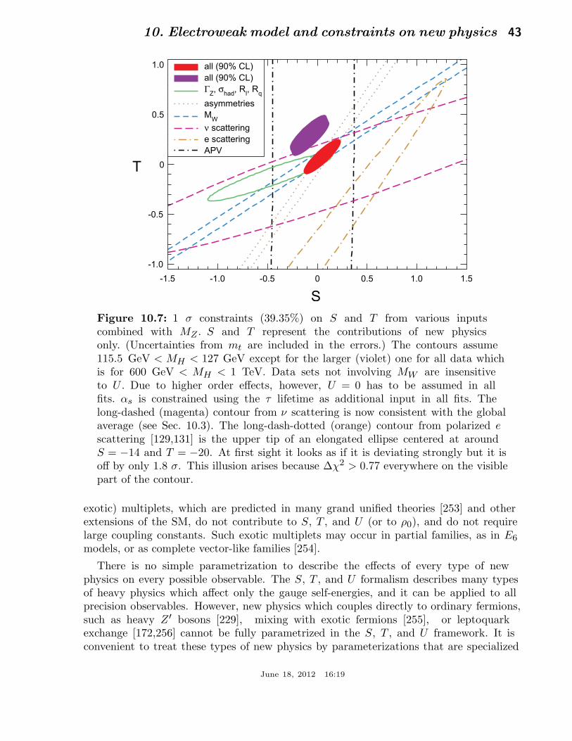
10. Electroweak model and constraints on new physics 43
Figure 10.7: 1 σ constraints (39.35%) on S and T from various inputscombined with MZ . S and T represent the contributions of new physicsonly. (Uncertainties from mt are included in the errors.) The contours assume115.5 GeV < MH < 127 GeV except for the larger (violet) one for all data whichis for 600 GeV < MH < 1 TeV. Data sets not involving MW are insensitiveto U . Due to higher order effects, however, U = 0 has to be assumed in allfits. αs is constrained using the τ lifetime as additional input in all fits. Thelong-dashed (magenta) contour from ν scattering is now consistent with the globalaverage (see Sec. 10.3). The long-dash-dotted (orange) contour from polarized escattering [129,131] is the upper tip of an elongated ellipse centered at aroundS = −14 and T = −20. At first sight it looks as if it is deviating strongly but it isoff by only 1.8 σ. This illusion arises because ∆χ2 > 0.77 everywhere on the visiblepart of the contour.
exotic) multiplets, which are predicted in many grand unified theories [253] and otherextensions of the SM, do not contribute to S, T , and U (or to ρ0), and do not requirelarge coupling constants. Such exotic multiplets may occur in partial families, as in E6
models, or as complete vector-like families [254].
There is no simple parametrization to describe the effects of every type of newphysics on every possible observable. The S, T , and U formalism describes many typesof heavy physics which affect only the gauge self-energies, and it can be applied to allprecision observables. However, new physics which couples directly to ordinary fermions,such as heavy Z ′ bosons [229], mixing with exotic fermions [255], or leptoquarkexchange [172,256] cannot be fully parametrized in the S, T , and U framework. It isconvenient to treat these types of new physics by parameterizations that are specialized
June 18, 2012 16:19
44 10. Electroweak model and constraints on new physics
to that particular class of theories (e.g., extra Z ′ bosons), or to consider specific models(which might contain, e.g., Z ′ bosons and exotic fermions with correlated parameters).Fits to Supersymmetric models are described in Ref. 244. Models involving strongdynamics (such as (extended) Technicolor) for EW breaking are considered in Ref. 257.The effects of compactified extra spatial dimensions at the TeV scale are reviewedin Ref. 258, and constraints on Little Higgs models in Ref. 259. The implications ofnon-standard Higgs sectors, e.g., involving Higgs singlets or triplets, are discussed inRef. 260, while additional Higgs doublets are considered in Ref. 230. Limits on newfour-Fermi operators and on leptoquarks using LEP 2 and lower energy data are givenin Refs. 172 and 261. Constraints on various types of new physics are reviewed inRefs. [7,128,149,161,262,263], and implications for the LHC in Ref. 264.
An alternate formalism [265] defines parameters, ǫ1, ǫ2, ǫ3, and ǫb in terms of the
specific observables MW /MZ , Γℓℓ, A(0,ℓ)FB , and Rb. The definitions coincide with those
for ǫi in Eqs. (10.65) and (10.66) for physics which affects gauge self-energies only, butthe ǫ’s now parametrize arbitrary types of new physics. However, the ǫ’s are not relatedto other observables unless additional model-dependent assumptions are made. Anotherapproach [266] parametrizes new physics in terms of gauge-invariant sets of operators.It is especially powerful in studying the effects of new physics on non-Abelian gaugevertices. The most general approach introduces deviation vectors [262]. Each type ofnew physics defines a deviation vector, the components of which are the deviations ofeach observable from its SM prediction, normalized to the experimental uncertainty. Thelength (direction) of the vector represents the strength (type) of new physics.
One of the best motivated kinds of physics beyond the SM besides Supersymmetryare extra Z ′ bosons [267]. They do not spoil the observed approximate gauge couplingunification, and appear copiously in many Grand Unified Theories (GUTs), mostSuperstring models [268], as well as in dynamical symmetry breaking [257] and LittleHiggs models [259]. For example, the SO(10) GUT contains an extra U(1) as canbe seen from its maximal subgroup, SU(5) × U(1)χ. Similarly, the E6 GUT containsthe subgroup SO(10) × U(1)ψ. The Zψ possesses only axial-vector couplings to theordinary fermions, and its mass is generally less constrained. The Zη boson is the linear
combination√
3/8Zχ −√
5/8Zψ. The ZLR boson occurs in left-right models with gaugegroup SU(3)C × SU(2)L × SU(2)R × U(1)B−L ⊂ SO(10), and the secluded ZS emergesin a supersymmetric bottom-up scenario [269]. The sequential ZSM boson is defined tohave the same couplings to fermions as the SM Z boson. Such a boson is not expectedin the context of gauge theories unless it has different couplings to exotic fermions thanthe ordinary Z boson. However, it serves as a useful reference case when comparingconstraints from various sources. It could also play the role of an excited state of theordinary Z boson in models with extra dimensions at the weak scale [258]. Finally,we consider a Superstring motivated Zstring boson appearing in a specific model [270].The potential Z ′ boson is in general a superposition of the SM Z and the new boson
June 18, 2012 16:19
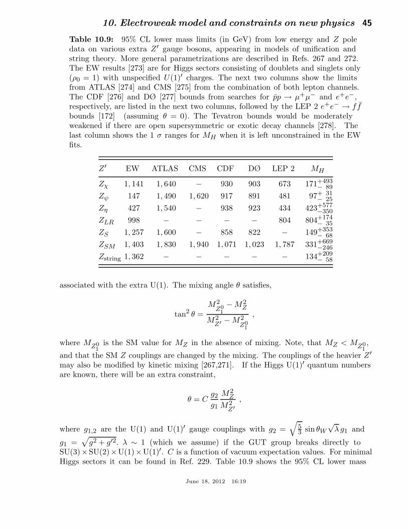
10. Electroweak model and constraints on new physics 45
Table 10.9: 95% CL lower mass limits (in GeV) from low energy and Z poledata on various extra Z ′ gauge bosons, appearing in models of unification andstring theory. More general parametrizations are described in Refs. 267 and 272.The EW results [273] are for Higgs sectors consisting of doublets and singlets only(ρ0 = 1) with unspecified U(1)′ charges. The next two columns show the limitsfrom ATLAS [274] and CMS [275] from the combination of both lepton channels.The CDF [276] and DØ [277] bounds from searches for pp → µ+µ− and e+e−,respectively, are listed in the next two columns, followed by the LEP 2 e+e− → f fbounds [172] (assuming θ = 0). The Tevatron bounds would be moderatelyweakened if there are open supersymmetric or exotic decay channels [278]. Thelast column shows the 1 σ ranges for MH when it is left unconstrained in the EWfits.
Z ′ EW ATLAS CMS CDF DØ LEP 2 MH
Zχ 1, 141 1, 640 − 930 903 673 171+493− 89
Zψ 147 1, 490 1, 620 917 891 481 97+ 31− 25
Zη 427 1, 540 − 938 923 434 423+577−350
ZLR 998 − − − − 804 804+174− 35
ZS 1, 257 1, 600 − 858 822 − 149+353− 68
ZSM 1, 403 1, 830 1, 940 1, 071 1, 023 1, 787 331+669−246
Zstring 1, 362 − − − − − 134+209− 58
associated with the extra U(1). The mixing angle θ satisfies,
tan2 θ =M2
Z01
− M2Z
M2Z′
− M2Z0
1
,
where MZ01
is the SM value for MZ in the absence of mixing. Note, that MZ < MZ01,
and that the SM Z couplings are changed by the mixing. The couplings of the heavier Z ′
may also be modified by kinetic mixing [267,271]. If the Higgs U(1)′ quantum numbersare known, there will be an extra constraint,
θ = Cg2
g1
M2Z
M2Z′
,
where g1,2 are the U(1) and U(1)′ gauge couplings with g2 =√
53 sin θW
√λ g1 and
g1 =√
g2 + g′2. λ ∼ 1 (which we assume) if the GUT group breaks directly toSU(3)×SU(2)×U(1)×U(1)′. C is a function of vacuum expectation values. For minimalHiggs sectors it can be found in Ref. 229. Table 10.9 shows the 95% CL lower mass
June 18, 2012 16:19
46 10. Electroweak model and constraints on new physics
limits [273] for ρ0 = 1 and 114.4 GeV ≤ MH ≤ 1 TeV. The last column shows the 1 σranges for MH when it is left unconstrained. In cases of specific minimal Higgs sectorswhere C is known, the Z ′ mass limits from the EW precision data are generally pushedinto the TeV region in which case they are still competitive with those from the LHC,and they are also competitive in the case of large g2 [279]. The limits on |θ| are typicallysmaller than a few ×10−3. For more details see [267,273,280,281] and the note on “The Z ′
Searches” in the Gauge & Higgs Boson Particle Listings. Also listed in Table 10.9 are thedirect lower limits on Z ′ production from the LHC [274,275] and the Tevatron [276,277],as well as the LEP 2 bounds [172].
Acknowledgments:
We are indebted to M. Davier, B. Malaescu, and K. Maltman for providing us withadditional information about their work in a form suitable to be included in our fits.We also thank R. H. Bernstein, K. S. McFarland, H. Schellman, and G. P. Zeller fordiscussions on the NuTeV analysis. This work was supported in part by CONACyT(Mexico) contract 82291–F and by PASPA (DGAPA–UNAM).
References:
1. S. L. Glashow, Nucl. Phys. 22, 579 (1961);S. Weinberg, Phys. Rev. Lett. 19, 1264 (1967);A. Salam, p. 367 of Elementary Particle Theory , ed. N. Svartholm (Almquist andWiksells, Stockholm, 1969);S.L. Glashow, J. Iliopoulos, and L. Maiani, Phys. Rev. D2, 1285 (1970).
2. CKMfitter Group: J. Charles et al., Eur. Phys. J. C41, 1 (2005);CKMfitter Group: S. T’Jampens et al., PoS ICHEP2010, 269 (2010).
3. For reviews, see the Section on “Higgs Bosons: Theory and Searches” in thisReview;J. Gunion et al., The Higgs Hunter’s Guide, (Addison-Wesley, Redwood City,1990);M. Carena and H.E. Haber, Prog. in Part. Nucl. Phys. 50, 63 (2003);A. Djouadi, Phys. Reports 457, 1 (2008).
4. For reviews, see E.D. Commins and P.H. Bucksbaum, Weak Interactions of Leptons
and Quarks, (Cambridge Univ. Press, 1983);G. Barbiellini and C. Santoni, Riv. Nuovo Cimento 9(2), 1 (1986);N. Severijns, M. Beck, and O. Naviliat-Cuncic, Rev. Mod. Phys. 78, 991 (2006);W. Fetscher and H.J. Gerber, p. 657 of Ref. 5;J. Deutsch and P. Quin, p. 706 of Ref. 5;P. Herczeg, p. 786 of Ref. 5;P. Herczeg, Prog. in Part. Nucl. Phys. 46, 413 (2001).
5. Precision Tests of the Standard Electroweak Model , ed. P. Langacker (WorldScientific, Singapore, 1995).
6. J. Erler and M.J. Ramsey-Musolf, Prog. in Part. Nucl. Phys. 54, 351 (2005).
7. P. Langacker, The Standard Model and Beyond , (CRC Press, New York, 2009).
8. T. Kinoshita, Quantum Electrodynamics, (World Scientific, Singapore, 1990).
9. S. G. Karshenboim, Phys. Reports 422, 1 (2005).
June 18, 2012 16:19
10. Electroweak model and constraints on new physics 47
10. P.J. Mohr, B.N. Taylor, and D.B. Newell, Rev. Mod. Phys. 80, 633 (2008); forupdates see http://physics.nist.gov/cuu/Constants/.
11. ALEPH, DELPHI, L3, OPAL, SLD, LEP Electroweak Working Group, SLDElectroweak and Heavy Flavour Groups: S. Schael et al., Phys. Reports 427, 257(2006); for updates see http://lepewwg.web.cern.ch/LEPEWWG/.
12. MuLan: D. M. Webber et al., Phys. Rev. Lett. 106, 041803 (2011).13. T. Kinoshita and A. Sirlin, Phys. Rev. 113, 1652 (1959).14. T. van Ritbergen and R.G. Stuart, Nucl. Phys. B564, 343 (2000);
M. Steinhauser and T. Seidensticker, Phys. Lett. B467, 271 (1999).15. Y. Nir, Phys. Lett. B221, 184 (1989).16. A. Pak and A. Czarnecki, Phys. Rev. Lett. 100, 241807 (2008).17. For a review, see S. Mele, arXiv:hep-ex/0610037.18. S. Fanchiotti, B. Kniehl, and A. Sirlin, Phys. Rev. D48, 307 (1993) and references
therein.19. J. Erler, Phys. Rev. D59, 054008 (1999).20. M. Davier et al., Eur. Phys. J. C71, 1515 (2011);
the quoted value uses additional information thankfully provided to us by theauthors in a private communication.
21. J. Erler, hep-ph/0005084.22. M. Steinhauser, Phys. Lett. B429, 158 (1998).23. A.D. Martin and D. Zeppenfeld, Phys. Lett. B345, 558 (1995).24. S. Eidelman and F. Jegerlehner, Z. Phys. C67, 585 (1995).25. B.V. Geshkenbein and V.L. Morgunov, Phys. Lett. B352, 456 (1995).26. H. Burkhardt and B. Pietrzyk, Phys. Lett. B356, 398 (1995).27. M.L. Swartz, Phys. Rev. D53, 5268 (1996).28. R. Alemany, M. Davier, and A. Hocker, Eur. Phys. J. C2, 123 (1998).29. N.V. Krasnikov and R. Rodenberg, Nuovo Cimento 111A, 217 (1998).30. M. Davier and A. Hocker, Phys. Lett. B419, 419 (1998).31. J.H. Kuhn and M. Steinhauser, Phys. Lett. B437, 425 (1998).32. M. Davier and A. Hocker, Phys. Lett. B435, 427 (1998).33. S. Groote et al., Phys. Lett. B440, 375 (1998).34. A.D. Martin, J. Outhwaite, and M.G. Ryskin, Phys. Lett. B492, 69 (2000).35. H. Burkhardt and B. Pietrzyk, Phys. Lett. B513, 46 (2001).36. J.F. de Troconiz and F.J. Yndurain, Phys. Rev. D65, 093002 (2002).37. F. Jegerlehner, Nucl. Phys. Proc. Suppl. 126, 325 (2004).38. K. Hagiwara et al., Phys. Rev. D69, 093003 (2004).39. H. Burkhardt and B. Pietrzyk, Phys. Rev. D72, 057501 (2005).40. K. Hagiwara et al., Phys. Lett. B649, 173 (2007).41. F. Jegerlehner, Nucl. Phys. Proc. Suppl. 181, 135 (2008).42. K. Hagiwara et al., J. Phys. G38, 085003 (2011).43. OPAL: K. Ackerstaff et al., Eur. Phys. J. C7, 571 (1999).44. CLEO: S. Anderson et al., Phys. Rev. D61, 112002 (2000).45. ALEPH: S. Schael et al., Phys. Reports 421, 191 (2005).46. Belle: M. Fujikawa et al.: Phys. Rev. D78, 072006 (2008).
June 18, 2012 16:19
48 10. Electroweak model and constraints on new physics
47. CMD-2: R.R. Akhmetshin et al., Phys. Lett. B578, 285 (2004);CMD-2: V.M. Aulchenko et al., JETP Lett. 82, 743 (2005);CMD-2: R.R. Akhmetshin et al., JETP Lett. 84, 413 (2006);CMD-2: R.R. Akhmetshin et al., Phys. Lett. B648, 28 (2007).
48. SND: M.N. Achasov et al., Sov. Phys. JETP 103, 380 (2006).
49. A.B. Arbuzov et al., JHEP 9812, 009 (1998);S. Binner, J.H. Kuhn, and K. Melnikov, Phys. Lett. B459, 279 (1999).
50. BaBar: B. Aubert et al., Phys. Rev. D70, 072004 (2004);BaBar: B. Aubert et al., Phys. Rev. D71, 052001 (2005);BaBar: B. Aubert et al., Phys. Rev. D73, 052003 (2006);BaBar: B. Aubert et al., Phys. Rev. D76, 092005 (2007);BaBar: B. Aubert et al., Phys. Rev. Lett. 103, 231801 (2009).
51. KLOE: F. Ambrosino et al., Phys. Lett. B670, 285 (2009);KLOE: F. Ambrosino et al., Phys. Lett. B700, 102 (2011).
52. See e.g., CMD and OLYA: L.M. Barkov et al., Nucl. Phys. B256, 365 (1985).
53. V.A. Novikov et al., Phys. Reports 41, 1 (1978).
54. J. Erler and M. Luo, Phys. Lett. B558, 125 (2003).
55. K. G. Chetyrkin et al., Phys. Rev. D80, 074010 (2009).
56. Tevatron Electroweak Working Group, CDF and DØ: arXiv:1107.5255 [hep-ex].
57. CMS: cdsweb.cern.ch/record/1356578/files/TOP-10-009-pas.pdf.
58. ATLAS: cdsweb.cern.ch/record/1376412/files/ATLAS-CONF-2011-120.pdf.
59. M. Beneke, Phys. Reports 317, 1 (1999).
60. K. G. Chetyrkin and M. Steinhauser, Nucl. Phys. B573, 617 (2000);K. Melnikov and T. van Ritbergen, Phys. Lett. B482, 99 (2000).
61. S.J. Brodsky, G.P. Lepage, and P.B. Mackenzie, Phys. Rev. D28, 228 (1983).
62. N. Gray et al., Z. Phys. C48, 673 (1990).
63. A. Sirlin, Phys. Rev. D22, 971 (1980);D.C. Kennedy et al., Nucl. Phys. B321, 83 (1989);D.Yu. Bardin et al., Z. Phys. C44, 493 (1989);W. Hollik, Fortsch. Phys. 38, 165 (1990);for reviews, see W. Hollik, pp. 37 and 117, and W. Marciano, p. 170 of Ref. 5.
64. V.A. Novikov, L.B. Okun, and M.I. Vysotsky, Nucl. Phys. B397, 35 (1993).
65. W. Hollik in Ref. 63 and references therein.
66. W.J. Marciano and J.L. Rosner, Phys. Rev. Lett. 65, 2963 (1990).
67. G. Degrassi, S. Fanchiotti, and A. Sirlin, Nucl. Phys. B351, 49 (1991).
68. G. Degrassi and A. Sirlin, Nucl. Phys. B352, 342 (1991).
69. P. Gambino and A. Sirlin, Phys. Rev. D49, 1160 (1994).
70. ZFITTER: A.B. Arbuzov et al., Comput. Phys. Commun. 174, 728 (2006) andreferences therein.
71. R. Barbieri et al., Nucl. Phys. B409, 105 (1993).
72. J. Fleischer, O.V. Tarasov, and F. Jegerlehner, Phys. Lett. B319, 249 (1993).
73. G. Degrassi, P. Gambino, and A. Vicini, Phys. Lett. B383, 219 (1996);G. Degrassi, P. Gambino, and A. Sirlin, Phys. Lett. B394, 188 (1997).
June 18, 2012 16:19
10. Electroweak model and constraints on new physics 49
74. A. Freitas et al., Phys. Lett. B495, 338 (2000) and ibid., 570, 260(E) (2003);M. Awramik and M. Czakon, Phys. Lett. B568, 48 (2003).
75. A. Freitas et al., Nucl. Phys. B632, 189 (2002) and ibid., 666, 305(E) (2003);M. Awramik and M. Czakon, Phys. Rev. Lett. 89, 241801 (2002);A. Onishchenko and O. Veretin, Phys. Lett. B551, 111 (2003).
76. M. Awramik et al., Phys. Rev. Lett. 93, 201805 (2004);W. Hollik, U. Meier, and S. Uccirati, Nucl. Phys. B731, 213 (2005).
77. M. Awramik, M. Czakon, and A. Freitas, JHEP 0611, 048 (2006);W. Hollik, U. Meier, and S. Uccirati, Nucl. Phys. B765, 154 (2007).
78. A. Djouadi and C. Verzegnassi, Phys. Lett. B195, 265 (1987);A. Djouadi, Nuovo Cimento 100A, 357 (1988).
79. K.G. Chetyrkin, J.H. Kuhn, and M. Steinhauser, Phys. Lett. B351, 331 (1995);L. Avdeev et al., Phys. Lett. B336, 560 (1994) and ibid., B349, 597(E) (1995).
80. B.A. Kniehl, J.H. Kuhn, and R.G. Stuart, Phys. Lett. B214, 621 (1988);B.A. Kniehl, Nucl. Phys. B347, 86 (1990);F. Halzen and B.A. Kniehl, Nucl. Phys. B353, 567 (1991);A. Djouadi and P. Gambino, Phys. Rev. D49, 3499 (1994) and ibid., 53, 4111(E)(1996).
81. K.G. Chetyrkin, J.H. Kuhn, and M. Steinhauser, Phys. Rev. Lett. 75, 3394 (1995).82. J.J. van der Bij et al., Phys. Lett. B498, 156 (2001).83. M. Faisst et al., Nucl. Phys. B665, 649 (2003).84. R. Boughezal, J.B. Tausk, and J.J. van der Bij, Nucl. Phys. B725, 3 (2005).85. A. Anselm, N. Dombey, and E. Leader, Phys. Lett. B312, 232 (1993).86. Y. Schroder and M. Steinhauser, Phys. Lett. B622, 124 (2005).87. K.G. Chetyrkin et al., Phys. Rev. Lett. 97, 102003 (2006);
R. Boughezal and M. Czakon, Nucl. Phys. B755, 221 (2006).88. J. Fleischer et al., Phys. Lett. B293, 437 (1992);
K.G. Chetyrkin, A. Kwiatkowski, and M. Steinhauser, Mod. Phys. Lett. A8, 2785(1993).
89. R. Harlander, T. Seidensticker, and M. Steinhauser, Phys. Lett. B426, 125 (1998);J. Fleischer et al., Phys. Lett. B459, 625 (1999).
90. M. Awramik et al., Nucl. Phys. B813, 174 (2009).91. A. Czarnecki and J.H. Kuhn, Phys. Rev. Lett. 77, 3955 (1996).92. Gfitter: H. Flacher et al., Eur. Phys. J. C60, 543 (2009).93. J.M. Conrad, M.H. Shaevitz, and T. Bolton, Rev. Mod. Phys. 70, 1341 (1998).94. Z. Berezhiani and A. Rossi, Phys. Lett. B535, 207 (2002);
S. Davidson et al., JHEP 0303, 011 (2003);A. Friedland, C. Lunardini and C. Pena-Garay, Phys. Lett. B594, 347 (2004).
95. J. Panman, p. 504 of Ref. 5.96. CHARM: J. Dorenbosch et al., Z. Phys. C41, 567 (1989).97. CALO: L.A. Ahrens et al., Phys. Rev. D41, 3297 (1990).98. CHARM II: P. Vilain et al., Phys. Lett. B335, 246 (1994).99. ILM: R.C. Allen et al., Phys. Rev. D47, 11 (1993);
LSND: L.B. Auerbach et al., Phys. Rev. D63, 112001 (2001).
June 18, 2012 16:19
50 10. Electroweak model and constraints on new physics
100. TEXONO: M. Deniz et al., Phys. Rev. D81, 072001 (2010).101. For reviews, see G.L. Fogli and D. Haidt, Z. Phys. C40, 379 (1988);
F. Perrier, p. 385 of Ref. 5.102. CDHS: A. Blondel et al., Z. Phys. C45, 361 (1990).103. CHARM: J.V. Allaby et al., Z. Phys. C36, 611 (1987).104. CCFR: K.S. McFarland et al., Eur. Phys. J. C1, 509 (1998).105. R.M. Barnett, Phys. Rev. D14, 70 (1976);
H. Georgi and H.D. Politzer, Phys. Rev. D14, 1829 (1976).106. LAB-E: S.A. Rabinowitz et al., Phys. Rev. Lett. 70, 134 (1993).107. E.A. Paschos and L. Wolfenstein, Phys. Rev. D7, 91 (1973).108. NuTeV: G.P. Zeller et al., Phys. Rev. Lett. 88, 091802 (2002).109. D. Mason et al., Phys. Rev. Lett. 99, 192001 (2007).110. S. Kretzer, D. Mason, and F. Olness, Phys. Rev. D65, 074010 (2002).111. J. Pumplin et al., JHEP 0207, 012 (2002);
S. Kretzer et al., Phys. Rev. Lett. 93, 041802 (2004).112. S. Alekhin, S.A. Kulagin, and R. Petti, Phys. Lett. B675, 433 (2009).113. W. Bentz et al., Phys. Lett. B693, 462 (2010).114. E. Sather, Phys. Lett. B274, 433 (1992);
E.N. Rodionov, A.W. Thomas, and J.T. Londergan, Mod. Phys. Lett. A9, 1799(1994).
115. A.D. Martin et al., Eur. Phys. J. C35, 325 (2004).116. J.T. Londergan and A.W. Thomas, Phys. Rev. D67, 111901 (2003).117. M. Gluck, P. Jimenez-Delgado, and E. Reya, Phys. Rev. Lett. 95, 022002 (2005).118. S. Kumano, Phys. Rev. D66, 111301 (2002);
S.A. Kulagin, Phys. Rev. D67, 091301 (2003);S.J. Brodsky, I. Schmidt, and J.J. Yang, Phys. Rev. D70, 116003 (2004);M. Hirai, S. Kumano, and T. H. Nagai, Phys. Rev. D71, 113007 (2005);G.A. Miller and A.W. Thomas, Int. J. Mod. Phys. A 20, 95 (2005).
119. I.C. Cloet, W. Bentz, and A.W. Thomas, Phys. Rev. Lett. 102, 252301 (2009).120. K.P.O. Diener, S. Dittmaier, and W. Hollik, Phys. Rev. D69, 073005 (2004);
A.B. Arbuzov, D.Y. Bardin, and L.V. Kalinovskaya, JHEP 0506, 078 (2005);K. Park, U. Baur, and D. Wackeroth, arXiv:0910.5013 [hep-ph].
121. K.P.O. Diener, S. Dittmaier, and W. Hollik, Phys. Rev. D72, 093002 (2005).122. B.A. Dobrescu and R.K. Ellis, Phys. Rev. D69, 114014 (2004).123. For a review, see S. Davidson et al., JHEP 0202, 037 (2002).124. SSF: C.Y. Prescott et al., Phys. Lett. B84, 524 (1979).125. E.J. Beise, M.L. Pitt, and D.T. Spayde, Prog. in Part. Nucl. Phys. 54, 289 (2005).126. S.L. Zhu et al., Phys. Rev. D62, 033008 (2000).127. P. Souder, p. 599 of Ref. 5.128. P. Langacker, p. 883 of Ref. 5.129. R.D. Young et al., Phys. Rev. Lett. 99, 122003 (2007).130. E. Derman and W.J. Marciano, Annals Phys. 121, 147 (1979).131. E158: P.L. Anthony et al., Phys. Rev. Lett. 95, 081601 (2005).132. J. Erler and M.J. Ramsey-Musolf, Phys. Rev. D72, 073003 (2005).
June 18, 2012 16:19
10. Electroweak model and constraints on new physics 51
133. A. Czarnecki and W.J. Marciano, Int. J. Mod. Phys. A 15, 2365 (2000).
134. K.S. McFarland, in the Proceedings of DIS 2008.
135. C. Bouchiat and C.A. Piketty, Phys. Lett. B128, 73 (1983).
136. Qweak: M.T. Gericke et al., AIP Conf. Proc. 1149, 237 (2009);the implications are discussed in Ref. 149.
137. For reviews and references to earlier work, see M.A. Bouchiat and L. Pottier,Science 234, 1203 (1986);B.P. Masterson and C.E. Wieman, p. 545 of Ref. 5.
138. Cesium (Boulder): C.S. Wood et al., Science 275, 1759 (1997).
139. Cesium (Paris): J. Guena, M. Lintz, and M.A. Bouchiat, Phys. Rev. A71, 042108(2005).
140. Thallium (Oxford): N.H. Edwards et al., Phys. Rev. Lett. 74, 2654 (1995);Thallium (Seattle): P.A. Vetter et al., Phys. Rev. Lett. 74, 2658 (1995).
141. Lead (Seattle): D.M. Meekhof et al., Phys. Rev. Lett. 71, 3442 (1993).
142. Bismuth (Oxford): M.J.D. MacPherson et al., Phys. Rev. Lett. 67, 2784 (1991).
143. V.A. Dzuba, V.V. Flambaum, and O.P. Sushkov, Phys. Lett. 141A, 147 (1989);S.A. Blundell, J. Sapirstein, and W.R. Johnson, Phys. Rev. D45, 1602 (1992);For reviews, see S.A. Blundell, W.R. Johnson, and J. Sapirstein, p. 577 of Ref. 5;J.S.M. Ginges and V.V. Flambaum, Phys. Reports 397, 63 (2004);J. Guena, M. Lintz, and M. A. Bouchiat, Mod. Phys. Lett. A20, 375 (2005);A. Derevianko and S.G. Porsev, Eur. Phys. J. A 32, 517 (2007).
144. V.A. Dzuba, V.V. Flambaum, and O.P. Sushkov, Phys. Rev. A56, R4357 (1997).
145. S.C. Bennett and C.E. Wieman, Phys. Rev. Lett. 82, 2484 (1999).
146. M.A. Bouchiat and J. Guena, J. Phys. (France) 49, 2037 (1988).
147. S. G. Porsev, K. Beloy, and A. Derevianko, Phys. Rev. Lett. 102, 181601 (2009).
148. A. Derevianko, Phys. Rev. Lett. 85, 1618 (2000);V.A. Dzuba, C. Harabati, and W.R. Johnson, Phys. Rev. A63, 044103 (2001);M.G. Kozlov, S.G. Porsev, and I.I. Tupitsyn, Phys. Rev. Lett. 86, 3260 (2001);W.R. Johnson, I. Bednyakov, and G. Soff, Phys. Rev. Lett. 87, 233001 (2001);A.I. Milstein and O.P. Sushkov, Phys. Rev. A66, 022108 (2002);V.A. Dzuba, V.V. Flambaum, and J.S. Ginges, Phys. Rev. D66, 076013 (2002);M.Y. Kuchiev and V.V. Flambaum, Phys. Rev. Lett. 89, 283002 (2002);A.I. Milstein, O.P. Sushkov, and I.S. Terekhov, Phys. Rev. Lett. 89, 283003 (2002);V.V. Flambaum and J.S.M. Ginges, Phys. Rev. A72, 052115 (2005).
149. J. Erler, A. Kurylov, and M.J. Ramsey-Musolf, Phys. Rev. D68, 016006 (2003).
150. P.G. Blunden, W. Melnitchouk, and A.W. Thomas, Phys. Rev. Lett. 107, 081801(2011).
151. V.A. Dzuba et al., J. Phys. B20, 3297 (1987).
152. Ya.B. Zel’dovich, Sov. Phys. JETP 6, 1184 (1958);for recent discussions, see V.V. Flambaum and D.W. Murray, Phys. Rev. C56,1641 (1997);W.C. Haxton and C.E. Wieman, Ann. Rev. Nucl. Part. Sci. 51, 261 (2001).
153. J.L. Rosner, Phys. Rev. D53, 2724 (1996).
June 18, 2012 16:19
52 10. Electroweak model and constraints on new physics
154. S.J. Pollock, E.N. Fortson, and L. Wilets, Phys. Rev. C46, 2587 (1992);B.Q. Chen and P. Vogel, Phys. Rev. C48, 1392 (1993).
155. R.W. Dunford and R.J. Holt, J. Phys. G34, 2099 (2007).156. O.O. Versolato et al., Hyperfine Interact. 199, 9 (2011).157. B.W. Lynn and R.G. Stuart, Nucl. Phys. B253, 216 (1985).158. Physics at LEP , ed. J. Ellis and R. Peccei, CERN 86–02, Vol. 1.159. PETRA: S.L. Wu, Phys. Reports 107, 59 (1984);
C. Kiesling, Tests of the Standard Theory of Electroweak Interactions, (Springer-Verlag, New York, 1988);R. Marshall, Z. Phys. C43, 607 (1989);Y. Mori et al., Phys. Lett. B218, 499 (1989);D. Haidt, p. 203 of Ref. 5.
160. For reviews, see D. Schaile, p. 215, and A. Blondel, p. 277 of Ref. 5; P. Langacker [7];and S. Riemann [161].
161. S. Riemann, Rept. on Prog. in Phys. 73, 126201 (2010).162. SLD: K. Abe et al., Phys. Rev. Lett. 84, 5945 (2000).163. SLD: K. Abe et al., Phys. Rev. Lett. 85, 5059 (2000).164. SLD: K. Abe et al., Phys. Rev. Lett. 86, 1162 (2001).165. DELPHI: P. Abreu et al., Z. Phys. C67, 1 (1995);
OPAL: K. Ackerstaff et al., Z. Phys. C76, 387 (1997).166. SLD: K. Abe et al., Phys. Rev. Lett. 78, 17 (1997).167. DØ: V.M. Abazov et al., Phys. Rev. D84, 012007 (2011).168. CDF: J. Han et al., arXiv:1110.0153 [hep-ex].169. CDF: D. Acosta et al., Phys. Rev. D71, 052002 (2005).170. H1: A. Aktas et al., Phys. Lett. B632, 35 (2006);
H1 and ZEUS: Z. Zhang, Nucl. Phys. Proc. Suppl. 191, 271 (2009).171. CMS: S. Chatrchyan et al., Phys. Rev. D84, 112002 (2011).172. ALEPH, DELPHI, L3, OPAL, and LEP Electroweak Working Group: J. Alcarez
et al., hep-ex/0612034.173. ALEPH, DELPHI, L3, OPAL, and the LEP Working Group for Higgs Boson
Searches: D. Abbaneo et al., Phys. Lett. B565, 61 (2003).174. J. Erler, Phys. Rev. D81, 051301 (R) (2010);
see also Ref. 92.175. A. Leike, T. Riemann, and J. Rose, Phys. Lett. B273, 513 (1991);
T. Riemann, Phys. Lett. B293, 451 (1992).176. A comprehensive report and further references can be found in K.G. Chetyrkin,
J.H. Kuhn, and A. Kwiatkowski, Phys. Reports 277, 189 (1996).177. J. Schwinger, Particles, Sources, and Fields, Vol. II, (Addison-Wesley, New York,
1973);K.G. Chetyrkin, A.L. Kataev, and F.V. Tkachev, Phys. Lett. B85, 277 (1979);M. Dine and J. Sapirstein, Phys. Rev. Lett. 43, 668 (1979);W. Celmaster and R.J. Gonsalves, Phys. Rev. Lett. 44, 560 (1980);S.G. Gorishnii, A.L. Kataev, and S.A. Larin, Phys. Lett. B259, 144 (1991);L.R. Surguladze, M.A. Samuel, Phys. Rev. Lett. 66, 560 (1991) and ibid., 2416(E).
June 18, 2012 16:19
10. Electroweak model and constraints on new physics 53
178. P.A. Baikov, K.G. Chetyrkin, and J.H. Kuhn, Phys. Rev. Lett. 101, 012002 (2008).
179. W. Bernreuther and W. Wetzel, Phys. Rev. D24, 2724 (1982);B.A. Kniehl, Phys. Lett. B237, 127 (1990);K.G. Chetyrkin, Phys. Lett. B307, 169 (1993);A.H. Hoang et al., Phys. Lett. B338, 330 (1994);S.A. Larin, T. van Ritbergen, and J.A.M. Vermaseren, Nucl. Phys. B438, 278(1995).
180. T.H. Chang, K.J.F. Gaemers, and W.L. van Neerven, Nucl. Phys. B202, 407(1980);J. Jersak, E. Laermann, and P.M. Zerwas, Phys. Rev. D25, 1218 (1982);S.G. Gorishnii, A.L. Kataev, and S.A. Larin, Nuovo Cimento 92, 117 (1986);K.G. Chetyrkin and J.H. Kuhn, Phys. Lett. B248, 359 (1990);K.G. Chetyrkin, J.H. Kuhn, and A. Kwiatkowski, Phys. Lett. B282, 221 (1992);K.G. Chetyrkin and J.H. Kuhn, Phys. Lett. B406, 102 (1997).
181. B.A. Kniehl and J.H. Kuhn, Nucl. Phys. B329, 547 (1990);K.G. Chetyrkin and A. Kwiatkowski, Phys. Lett. B319, 307 (1993);S.A. Larin, T. van Ritbergen, and J.A.M. Vermaseren, Phys. Lett. B320, 159(1994);K.G. Chetyrkin and O.V. Tarasov, Phys. Lett. B327, 114 (1994).
182. A.L. Kataev, Phys. Lett. B287, 209 (1992).
183. D. Albert et al., Nucl. Phys. B166, 460 (1980);F. Jegerlehner, Z. Phys. C32, 425 (1986);A. Djouadi, J.H. Kuhn, and P.M. Zerwas, Z. Phys. C46, 411 (1990);A. Borrelli et al., Nucl. Phys. B333, 357 (1990).
184. A.A. Akhundov, D.Yu. Bardin, and T. Riemann, Nucl. Phys. B276, 1 (1986);W. Beenakker and W. Hollik, Z. Phys. C40, 141 (1988);B.W. Lynn and R.G. Stuart, Phys. Lett. B352, 676 (1990);J. Bernabeu, A. Pich, and A. Santamaria, Phys. Lett. B200, 569 (1988) and Nucl.Phys. B363, 326 (1991).
185. Tevatron Electroweak Working Group, CDF and DØ: 1003.2826 [hep-ex].
186. E. Braaten, S. Narison, and A. Pich, Nucl. Phys. B373, 581 (1992).
187. F. Le Diberder and A. Pich, Phys. Lett. B286, 147 (1992).
188. M. Beneke and M. Jamin, JHEP 0809, 044 (2008).
189. E. Braaten and C.S. Li, Phys. Rev. D42, 3888 (1990).
190. J. Erler, Rev. Mex. Fis. 50, 200 (2004).
191. D. Boito et al., Phys. Rev. D84, 113006 (2011);D. Boito et al., arXiv:1203.3146 [hep-ph].
192. J. Erler, arXiv:1102.5520 [hep-ph].
193. M. Davier et al., Eur. Phys. J. C56, 305 (2008);K. Maltman and T. Yavin, Phys. Rev. D78, 094020 (2008).
194. E821: G.W. Bennett et al., Phys. Rev. Lett. 92, 161802 (2004).
195. T. Kinoshita and M. Nio, Phys. Rev. D70, 113001 (2004);M. Passera, J. Phys. G31, R75 (2005);T. Kinoshita, Nucl. Phys. Proc. Suppl. 144, 206 (2005).
June 18, 2012 16:19
54 10. Electroweak model and constraints on new physics
196. G. Li, R. Mendel, and M.A. Samuel, Phys. Rev. D47, 1723 (1993);S. Laporta and E. Remiddi, Phys. Lett. B301, 440 (1993);S. Laporta and E. Remiddi, Phys. Lett. B379, 283 (1996);A. Czarnecki and M. Skrzypek, Phys. Lett. B449, 354 (1999).
197. J. Erler and M. Luo, Phys. Rev. Lett. 87, 071804 (2001).
198. A.L. Kataev, Nucl. Phys. Proc. Suppl. 155, 369 (2006);T. Kinoshita and M. Nio, Phys. Rev. D73, 053007 (2006).
199. For reviews, see V.W. Hughes and T. Kinoshita, Rev. Mod. Phys. 71, S133 (1999);A. Czarnecki and W.J. Marciano, Phys. Rev. D64, 013014 (2001);T. Kinoshita, J. Phys. G29, 9 (2003);M. Davier and W.J. Marciano, Ann. Rev. Nucl. Part. Sci. 54, 115 (2004);J.P. Miller, E. de Rafael, and B.L. Roberts, Rept. Prog. Phys. 70, 795 (2007);F. Jegerlehner, Acta Phys. Polon. B38, 3021 (2007).
200. S.J. Brodsky and J.D. Sullivan, Phys. Rev. D156, 1644 (1967);T. Burnett and M.J. Levine, Phys. Lett. B24, 467 (1967);R. Jackiw and S. Weinberg, Phys. Rev. D5, 2473 (1972);I. Bars and M. Yoshimura, Phys. Rev. D6, 374 (1972);K. Fujikawa, B.W. Lee, and A.I. Sanda, Phys. Rev. D6, 2923 (1972);G. Altarelli, N. Cabibbo, and L. Maiani, Phys. Lett. B40, 415 (1972);W.A. Bardeen, R. Gastmans, and B.E. Laurup, Nucl. Phys. B46, 315 (1972).
201. T.V. Kukhto et al., Nucl. Phys. B371, 567 (1992);S. Peris, M. Perrottet, and E. de Rafael, Phys. Lett. B355, 523 (1995);A. Czarnecki, B. Krause, and W.J. Marciano, Phys. Rev. D52, 2619 (1995);A. Czarnecki, B. Krause, and W.J. Marciano, Phys. Rev. Lett. 76, 3267 (1996).
202. G. Degrassi and G. Giudice, Phys. Rev. D58, 053007 (1998).
203. V. Cirigliano, G. Ecker, and H. Neufeld, JHEP 0208, 002 (2002);K. Maltman and C.E. Wolfe, Phys. Rev. D73, 013004 (2006);M. Davier et al., Eur. Phys. J. C66, 127 (2010).
204. W.J. Marciano and A. Sirlin, Phys. Rev. Lett. 61, 1815 (1988).
205. S. Ghozzi and F. Jegerlehner, Phys. Lett. B583, 222 (2004).
206. K. Melnikov and A. Vainshtein, Phys. Rev. D70, 113006 (2004).
207. J. Erler and G. Toledo Sanchez, Phys. Rev. Lett. 97, 161801 (2006).
208. M. Knecht and A. Nyffeler, Phys. Rev. D65, 073034 (2002).
209. M. Hayakawa and T. Kinoshita, hep-ph/0112102;J. Bijnens, E. Pallante, and J. Prades, Nucl. Phys. B626, 410 (2002);A recent discussion is in J. Bijnens and J. Prades, Mod. Phys. Lett. A22, 767(2007).
210. J. Prades, E. de Rafael, and A. Vainshtein, 0901.0306 [hep-ph].
211. B. Krause, Phys. Lett. B390, 392 (1997).
212. J.L. Lopez, D.V. Nanopoulos, and X. Wang, Phys. Rev. D49, 366 (1994);for recent reviews, see Ref. 199.
213. U. Amaldi et al., Phys. Rev. D36, 1385 (1987);G. Costa et al., Nucl. Phys. B297, 244 (1988);
June 18, 2012 16:19

10. Electroweak model and constraints on new physics 55
P. Langacker and M. Luo, Phys. Rev. D44, 817 (1991);J. Erler and P. Langacker, Phys. Rev. D52, 441 (1995).
214. Tevatron Electroweak Working Group, CDF and DØ: 0908.1374 [hep-ex].215. J. Erler, arXiv:1201.0695 [hep-ph].216. F. James and M. Roos, Comput. Phys. Commun. 10, 343 (1975).217. For a more recent study, see J. Cao and J.M. Yang, JHEP 0812, 006 (2008).218. J. Erler, J.L. Feng, and N. Polonsky, Phys. Rev. Lett. 78, 3063 (1997).219. D. Choudhury, T.M.P. Tait, and C.E.M. Wagner, Phys. Rev. D65, 053002 (2002).220. J. Erler and P. Langacker, Phys. Rev. Lett. 84, 212 (2000).221. P. Langacker and M. Plumacher, Phys. Rev. D62, 013006 (2000).222. DELPHI: P. Abreu et al., Eur. Phys. J. C10, 415 (1999).223. P. Langacker and N. Polonsky, Phys. Rev. D52, 3081 (1995);
J. Bagger, K.T. Matchev, and D. Pierce, Phys. Lett. B348, 443 (1995).224. F. Gianotti, CERN public seminar, ATLAS-CONF-2011-163.225. CDF and DØ: arXiv:1107.5518 [hep-ex].226. J. Erler, Phys. Rev. D63, 071301 (R) (2001).227. G. Tonelli, CERN public seminar, CMS-HIG-11-032.228. M. Veltman, Nucl. Phys. B123, 89 (1977);
M. Chanowitz, M.A. Furman, and I. Hinchliffe, Phys. Lett. B78, 285 (1978);The two-loop correction has been obtained by J.J. van der Bij and F. Hoogeveen,Nucl. Phys. B283, 477 (1987).
229. P. Langacker and M. Luo, Phys. Rev. D45, 278 (1992) and refs. therein.230. A. Denner, R.J. Guth, and J.H. Kuhn, Phys. Lett. B240, 438 (1990);
W. Grimus et al., J. Phys. G 35, 075001 (2008);H. E. Haber and D. O’Neil, Phys. Rev. D83, 055017 (2011).
231. S. Bertolini and A. Sirlin, Phys. Lett. B257, 179 (1991).232. M. Peskin and T. Takeuchi, Phys. Rev. Lett. 65, 964 (1990);
M. Peskin and T. Takeuchi, Phys. Rev. D46, 381 (1992);M. Golden and L. Randall, Nucl. Phys. B361, 3 (1991).
233. D. Kennedy and P. Langacker, Phys. Rev. D44, 1591 (1991).234. G. Altarelli and R. Barbieri, Phys. Lett. B253, 161 (1990).235. B. Holdom and J. Terning, Phys. Lett. B247, 88 (1990).236. B.W. Lynn, M.E. Peskin, and R.G. Stuart, p. 90 of Ref. 158.237. An alternative formulation is given by K. Hagiwara et al., Z. Phys. C64, 559
(1994), and ibid., 68, 352(E) (1995);K. Hagiwara, D. Haidt, and S. Matsumoto, Eur. Phys. J. C2, 95 (1998).
238. I. Maksymyk, C.P. Burgess, and D. London, Phys. Rev. D50, 529 (1994);C.P. Burgess et al., Phys. Lett. B326, 276 (1994).
239. R. Barbieri et al., Nucl. Phys. B703, 127 (2004).240. K. Lane, hep-ph/0202255.241. E. Gates and J. Terning, Phys. Rev. Lett. 67, 1840 (1991);
R. Sundrum and S.D.H. Hsu, Nucl. Phys. B391, 127 (1993);R. Sundrum, Nucl. Phys. B395, 60 (1993);M. Luty and R. Sundrum, Phys. Rev. Lett. 70, 529 (1993);
June 18, 2012 16:19
56 10. Electroweak model and constraints on new physics
T. Appelquist and J. Terning, Phys. Lett. B315, 139 (1993);D.D. Dietrich, F. Sannino, and K. Tuominen, Phys. Rev. D72, 055001 (2005);N.D. Christensen and R. Shrock, Phys. Lett. B632, 92 (2006);M. Harada, M. Kurachi, and K. Yamawaki, Prog. Theor. Phys. 115, 765 (2006).
242. H. Georgi, Nucl. Phys. B363, 301 (1991);M.J. Dugan and L. Randall, Phys. Lett. B264, 154 (1991).
243. R. Barbieri et al., Nucl. Phys. B341, 309 (1990).
244. J. Erler and D.M. Pierce, Nucl. Phys. B526, 53 (1998);G.C. Cho and K. Hagiwara, Nucl. Phys. B574, 623 (2000);G. Altarelli et al., JHEP 0106, 018 (2001);S. Heinemeyer, W. Hollik, and G. Weiglein, Phys. Reports 425, 265 (2006);S.P. Martin, K. Tobe, and J.D. Wells, Phys. Rev. D71, 073014 (2005);G. Marandella, C. Schappacher, and A. Strumia, Nucl. Phys. B715, 173 (2005);S. Heinemeyer et al., JHEP 0608, 052 (2006);M.J. Ramsey-Musolf and S. Su, Phys. Reports 456, 1 (2008);J.R. Ellis et al., JHEP 0708, 083 (2007);A. Djouadi, Phys. Reports 459, 1 (2008);S. Heinemeyer et al., JHEP 0804, 039 (2008).
245. M.E. Peskin and J.D. Wells, Phys. Rev. D64, 093003 (2001).
246. G.D. Kribs et al., Phys. Rev. D76, 075016 (2007).
247. H.J. He, N. Polonsky, and S. Su, Phys. Rev. D64, 053004 (2001);V.A. Novikov et al., Sov. Phys. JETP 76, 127 (2002);S.S. Bulanov et al., Yad. Fiz. 66, 2219 (2003) and refs. therein.
248. J. Maalampi and M. Roos, Phys. Reports 186, 53 (1990).
249. J. Erler and P. Langacker, Phys. Rev. Lett. 105, 031801 (2010).
250. CDF and DØ: D. Benjamin, arXiv:1108.3331 [hep-ex].
251. ATLAS: http://atlas.ch/news/2011/Higgs-note.pdf.
252. Z. Murdock, S. Nandi and Z. Tavartkiladze, Phys. Lett. B668, 303 (2008).
253. For reviews, see the Section on “Grand Unified Theories” in this Review;P. Langacker, Phys. Reports 72, 185 (1981);J.L. Hewett and T.G. Rizzo, Phys. Reports 183, 193 (1989);for collider implications, see T.C. Andre and J.L. Rosner, Phys. Rev. D69, 035009(2004);J. Kang, P. Langacker and B.D. Nelson, Phys. Rev. D77, 035003 (2008).
254. S.P. Martin, Phys. Rev. D81, 035004 (2010);P.W. Graham et al., Phys. Rev. D81, 055016 (2010).
255. P. Langacker and D. London, Phys. Rev. D38, 886 (1988);D. London, p. 951 of Ref. 5;a recent analysis is F. del Aguila, J. de Blas and M. Perez-Victoria, Phys. Rev.D78, 013010 (2008).
256. M. Chemtob, Prog. in Part. Nucl. Phys. 54, 71 (2005);R. Barbier et al., Phys. Reports 420, 1 (2005).
June 18, 2012 16:19

10. Electroweak model and constraints on new physics 57
257. R.S. Chivukula and E.H. Simmons, Phys. Rev. D66, 015006 (2002);C.T. Hill and E.H. Simmons, Phys. Reports 381, 235 (2003);R.S. Chivukula et al., Phys. Rev. D70, 075008 (2004).
258. K. Agashe et al., JHEP 0308, 050 (2003);M. Carena et al., Phys. Rev. D68, 035010 (2003);I. Gogoladze and C. Macesanu, Phys. Rev. D74, 093012 (2006);I. Antoniadis, hep-th/0102202 see also the note on “Extra Dimensions” in theSearches Particle Listings.
259. T. Han, H.E. Logan, and L.T. Wang, JHEP 0601, 099 (2006);M. Perelstein, Prog. in Part. Nucl. Phys. 58, 247 (2007).
260. E. Accomando et al., arXiv:hep-ph/0608079;V. Barger et al., Phys. Rev. D77, 035005 (2008);W. Grimus et al., Nucl. Phys. B801, 81 (2008);M. Maniatis, Int. J. Mod. Phys. A25, 3505 (2010);U. Ellwanger, C. Hugonie, and A.M. Teixeira, Phys. Reports 496, 1 (2010);M.C. Chen, S. Dawson, and C.B. Jackson, Phys. Rev. D78, 093001 (2008).
261. G.C. Cho, K. Hagiwara, and S. Matsumoto, Eur. Phys. J. C5, 155 (1998);K. Cheung, Phys. Lett. B517, 167 (2001);Z. Han and W. Skiba, Phys. Rev. D71, 075009 (2005).
262. P. Langacker, M. Luo, and A.K. Mann, Rev. Mod. Phys. 64, 87 (1992);M. Luo, p. 977 of Ref. 5.
263. F.S. Merritt et al., p. 19 of Particle Physics: Perspectives and Opportunities:
Report of the DPF Committee on Long Term Planning , ed. R. Peccei et al. (WorldScientific, Singapore, 1995);M. Baak et al., arXiv:1107.0975 [hep-ph].
264. D.E. Morrissey, T. Plehn, and T.M.P. Tait, arXiv:0912.3259 [hep-ph].
265. G. Altarelli, R. Barbieri, and S. Jadach, Nucl. Phys. B369, 3 (1992) and ibid.,B376, 444(E) (1992).
266. A. De Rujula et al., Nucl. Phys. B384, 3 (1992);K. Hagiwara et al., Phys. Rev. D48, 2182 (1993);C.P. Burgess et al., Phys. Rev. D49, 6115 (1994);Z. Han and W. Skiba, Phys. Rev. D71, 075009 (2005);G. Cacciapaglia et al., Phys. Rev. D74, 033011 (2006);V. Bernard et al., JHEP 0801, 015 (2008);Z. Han, Int. J. Mod. Phys. A 23, 2653 (2008).
267. For reviews, see A. Leike, Phys. Reports 317, 143 (1999);P. Langacker, Rev. Mod. Phys. 81, 1199 (2009).
268. M. Cvetic and P. Langacker, Phys. Rev. D54, 3570 (1996).
269. J. Erler, P. Langacker, and T. Li, Phys. Rev. D66, 015002 (2002).
270. S. Chaudhuri et al., Nucl. Phys. B456, 89 (1995);G. Cleaver et al., Phys. Rev. D59, 055005 (1999).
271. B. Holdom, Phys. Lett. B166, 196 (1986).
272. M. Carena et al., Phys. Rev. D70, 093009 (2004).
273. J. Erler, P. Langacker, S. Munir and E. Rojas, JHEP 0908, 017 (2009).
June 18, 2012 16:19
58 10. Electroweak model and constraints on new physics
274. ATLAS: G. Aad et al., Phys. Rev. Lett. 107, 272002 (2011).275. CMS: cdsweb.cern.ch/record/1369192/files/EXO-11-019-pas.pdf.276. CDF: T. Aaltonen et al., Phys. Rev. Lett. 106, 121801 (2011).277. DØ: V.M. Abazov et al., Phys. Lett. B695, 88 (2011).278. J. Kang and P. Langacker, Phys. Rev. D71, 035014 (2005);
C. -F. Chang, K. Cheung, and T. -C. Yuan, JHEP 1109, 058 (2011).279. J. Erler et al., JHEP 1111, 076 (2011).280. F. del Aguila, J. de Blas, and M. Perez-Victoria, JHEP 1009, 033 (2010).281. T. Appelquist, B.A. Dobrescu, and A.R. Hopper, Phys. Rev. D68, 035012 (2003);
R.S. Chivukula et al., Phys. Rev. D69, 015009 (2004).
June 18, 2012 16:19