10.34: Numerical Methods Applied to Chemical Engineering

10.34: Numerical Methods Applied to

Chemical Engineering

Lecture 3: Existence and uniqueness of solutions

Four fundamental subspaces

1

Recap

• Scalars, vectors, and matrices

• Transformations/maps

• Determinant

• Induced norms

• Condition number

2

Recap

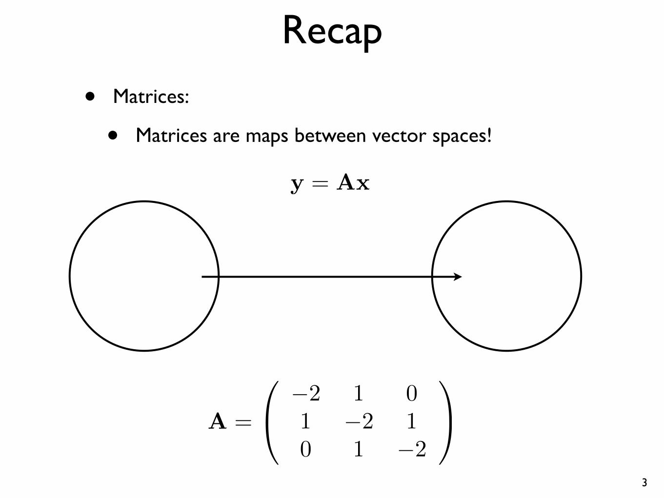
• Matrices:

• Matrices are maps between vector spaces!

y = Ax

0

@-2 1 0

1

A 1 0

A = -2 1 1 -2

3

Recap

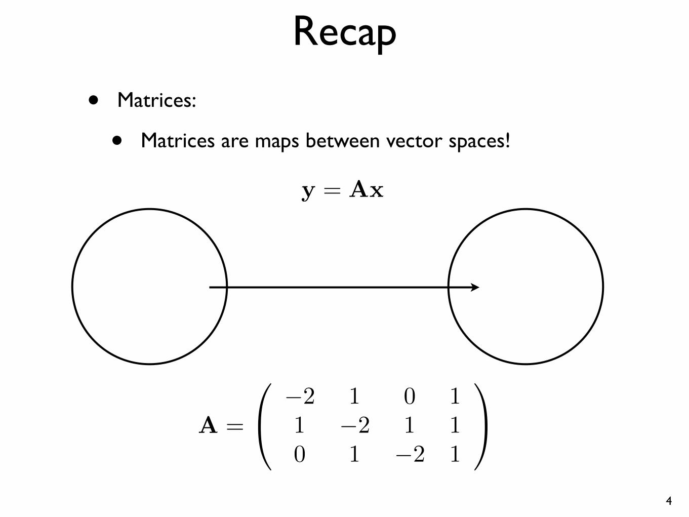
• Matrices:


y = Ax

0 -2 1 0 1

1

A = 1 -2 1 1 @ A

0 1 -2 1

4

Recap

• Matrices:


y = Ax

0 -2 1 0

1

1 -2 1 A =

B CB0 1 -2

C@ A

1 1 1 5

Recap

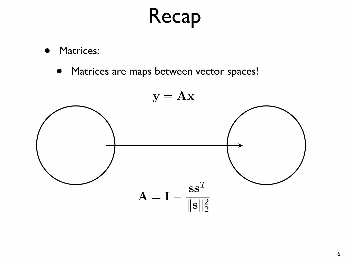
• Matrices:


y = Ax

TssA = I - ksk22

6

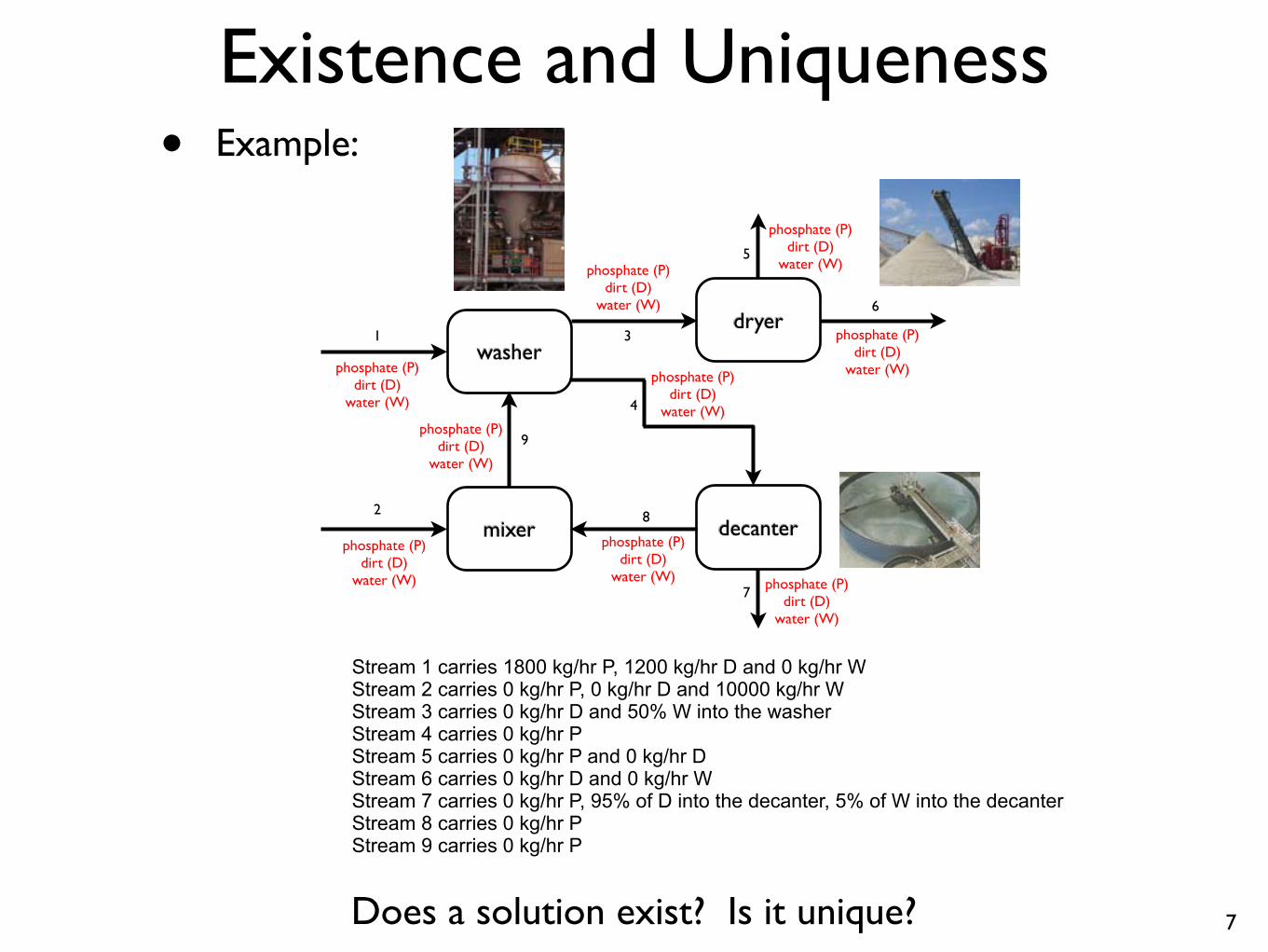
Existence and Uniqueness • Example:

phosphate (P) dirt (D)

water (W)

washer dryer

decanter mixer

1

2

3

4

5

6

7

8

9


water (W)


water (W)


water (W)


water (W)


water (W)


water (W)


water (W)


water (W)

Stream 1 carries 1800 kg/hr P, 1200 kg/hr D and 0 kg/hr W Stream 2 carries 0 kg/hr P, 0 kg/hr D and 10000 kg/hr W Stream 3 carries 0 kg/hr D and 50% W into the washer Stream 4 carries 0 kg/hr P Stream 5 carries 0 kg/hr P and 0 kg/hr D Stream 6 carries 0 kg/hr D and 0 kg/hr W Stream 7 carries 0 kg/hr P, 95% of D into the decanter, 5% of W into the decanter Stream 8 carries 0 kg/hr P Stream 9 carries 0 kg/hr P

Does a solution exist? Is it unique? 7

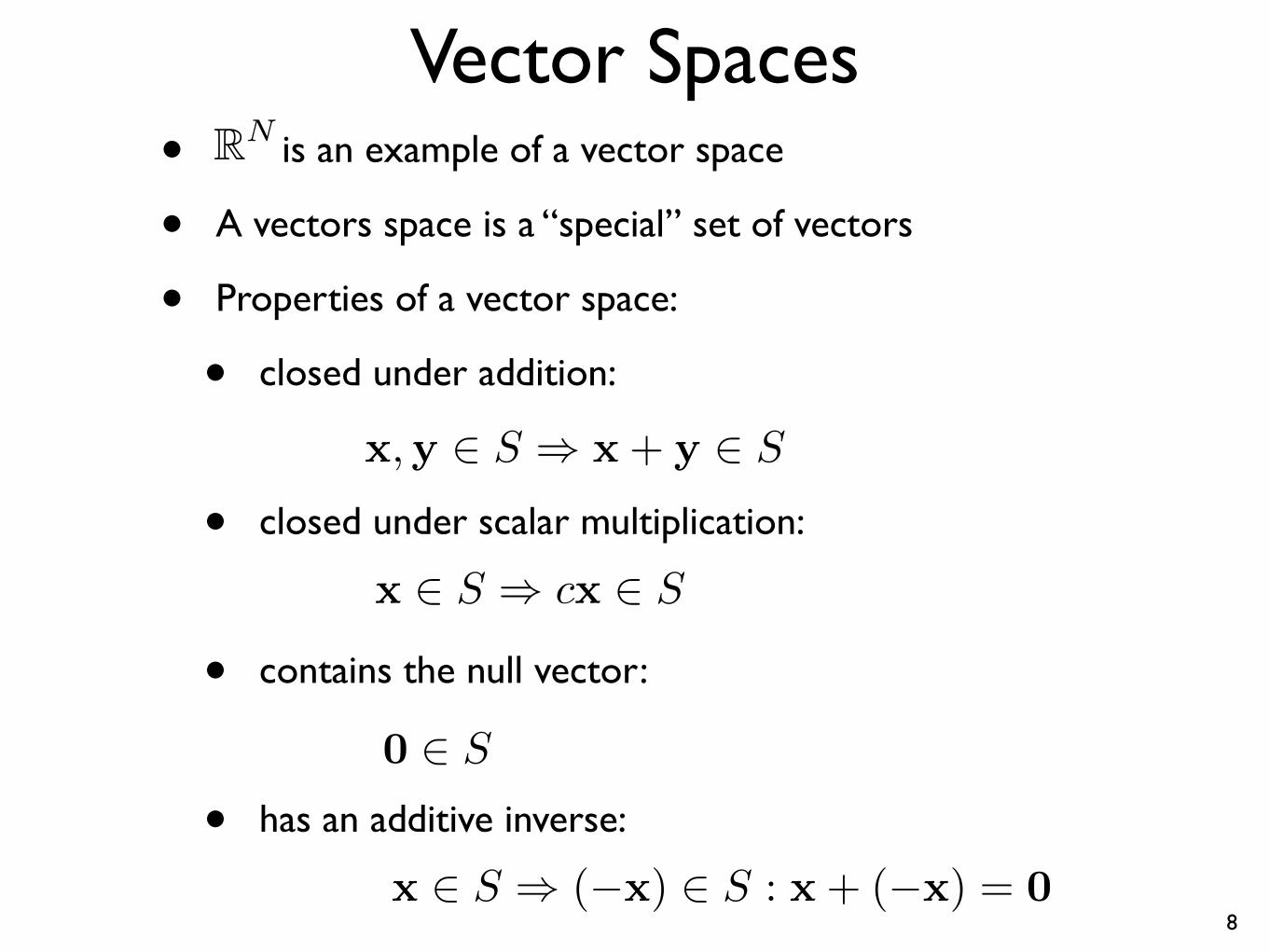
Vector Spaces RN• is an example of a vector space

• A vectors space is a “special” set of vectors

• Properties of a vector space:

• closed under addition:

x, y 2 S ) x + y 2 S

• closed under scalar multiplication:

x 2 S ) cx 2 S

• contains the null vector:

0 2 S

• has an additive inverse:

x 2 S ) (-x) 2 S : x + (-x) = 0 8

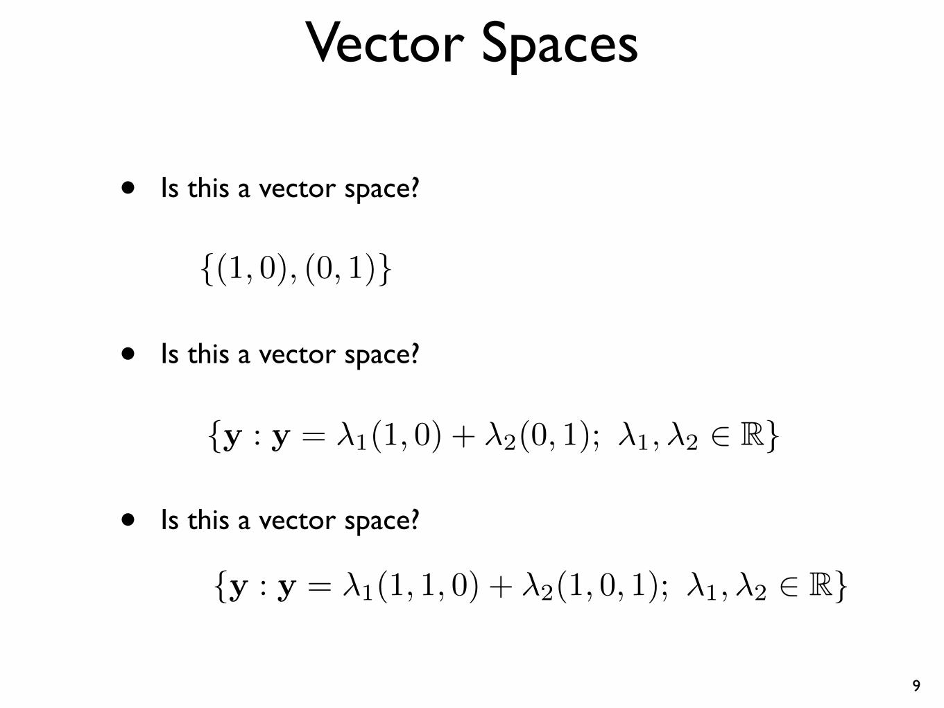
Vector Spaces

• Is this a vector space?

{(1, 0), (0, 1)}


{y : y = �1(1, 0) + �2(0, 1); �1, �2 2 R}


{y : y = �1(1, 1, 0) + �2(1, 0, 1); �1, �2 2 R}

9

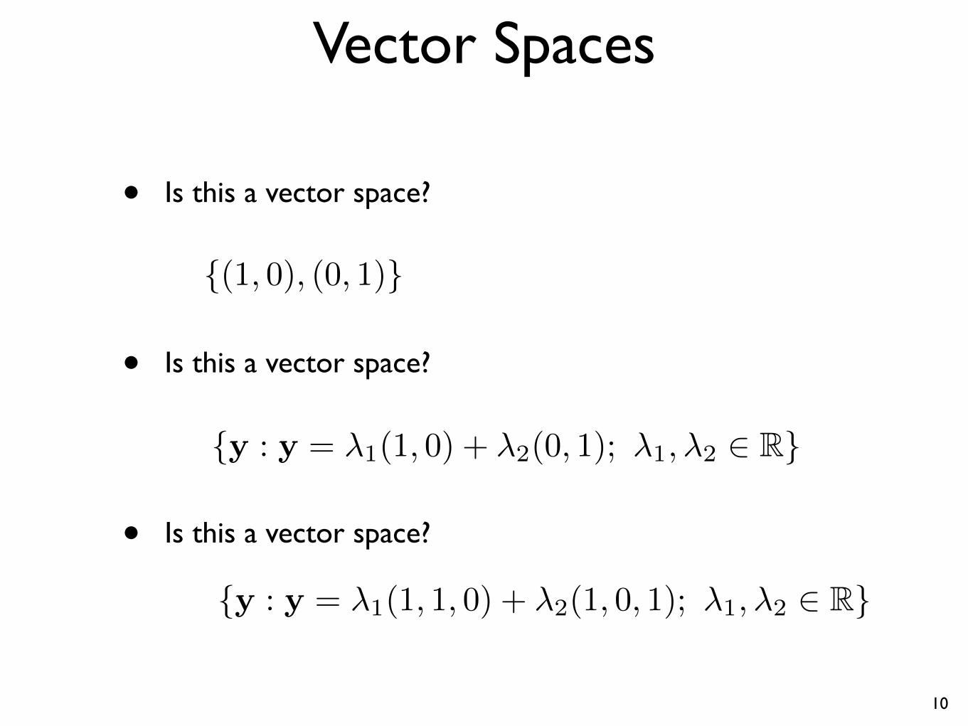
Vector Spaces




10

{(1, 0), (0, 1)}

{y : y = �1(1, 0) + �2(0, 1); �1,�2 2 R}

{y : y = �1(1, 1, 0) + �2(1, 0, 1); �1,�2 2 R}

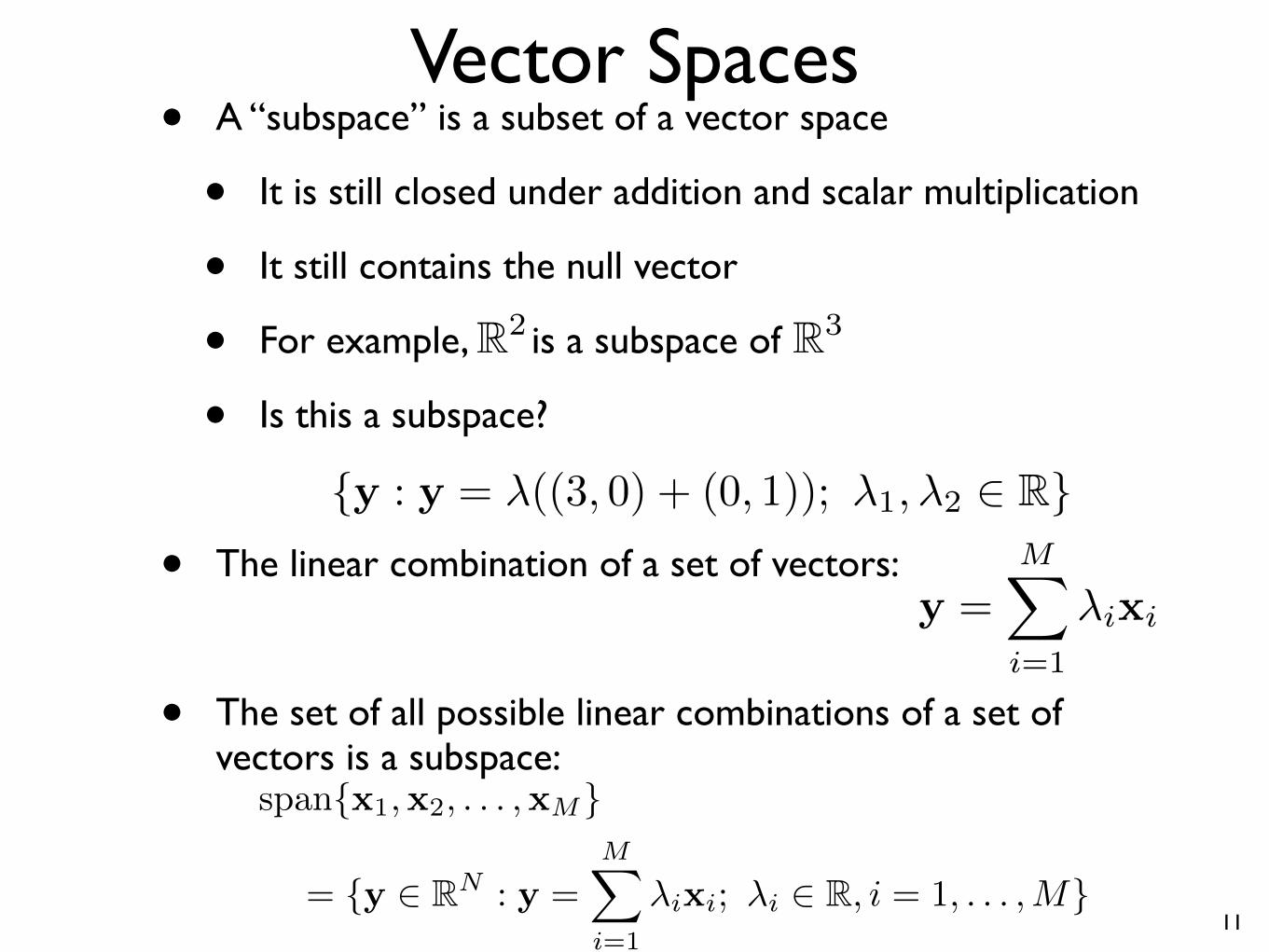
Vector Spaces • A “subspace” is a subset of a vector space

• It is still closed under addition and scalar multiplication

• It still contains the null vector

• For example, R2 is a subspace of R3

• Is this a subspace?

{y : y = A((3, 0) + (0, 1)); A1, A2 2 R} M• The linear combination of a set of vectors:

y = X

Aixi

i=1

• The set of all possible linear combinations of a set of vectors is a subspace:

span{x1,x2, . . . ,xM }M

= {y 2 RN : y = X

Aixi; Ai 2 R, i = 1, . . . ,M}i=1

11

Linear Dependence

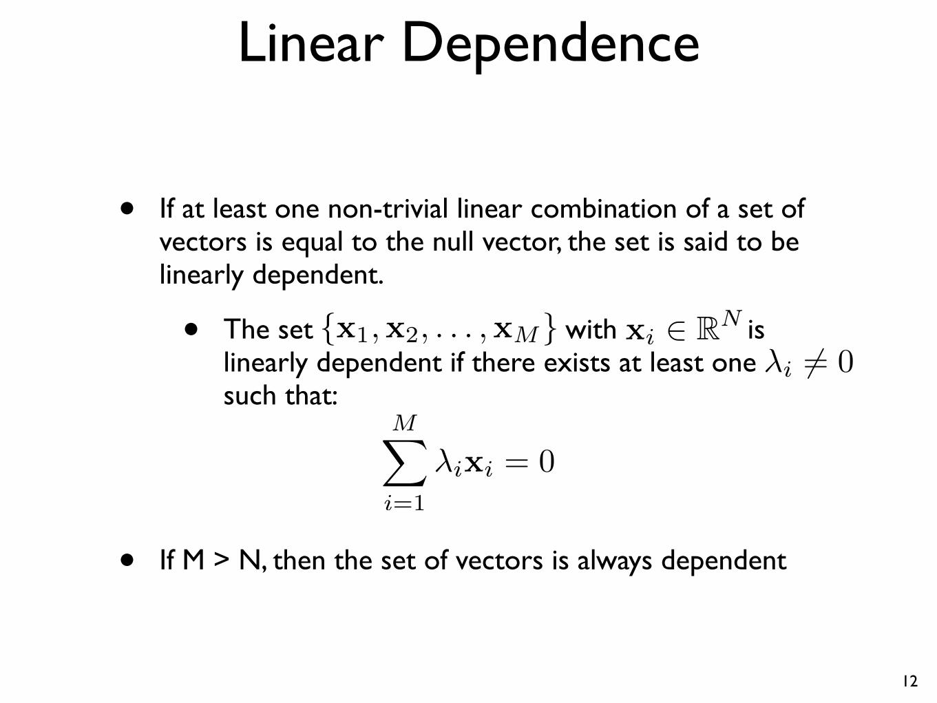
• If at least one non-trivial linear combination of a set of vectors is equal to the null vector, the set is said to be linearly dependent.

• The set {x1,x2, . . . ,xM } with xi 2 RN is

linearly dependent if there exists at least one Ai = 06such that:

MX Aixi = 0

i=1

• If M > N, then the set of vectors is always dependent

12

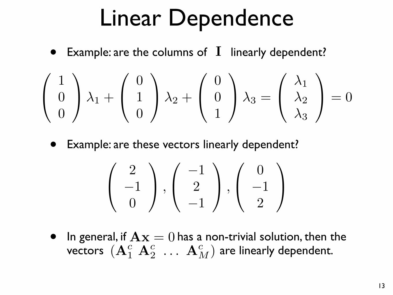
Linear Dependence • Example: are the columns of I linearly dependent?

1

A100

0

@ 1 +

1

A010

0

@ 2 +

1

A001

0

@ 3 =

0

@

1

A 1

2 = 0 3

• Example: are these vectors linearly dependent? 0 1

A,

0

@ -1 2 -1

1

A,

0

@

12 0

@ A-1 0

-1 2

• In general, if Ax = 0 has a non-trivial solution, then the

vectors (Ac 1 Ac

2 . . . AcM) are linearly dependent.

13

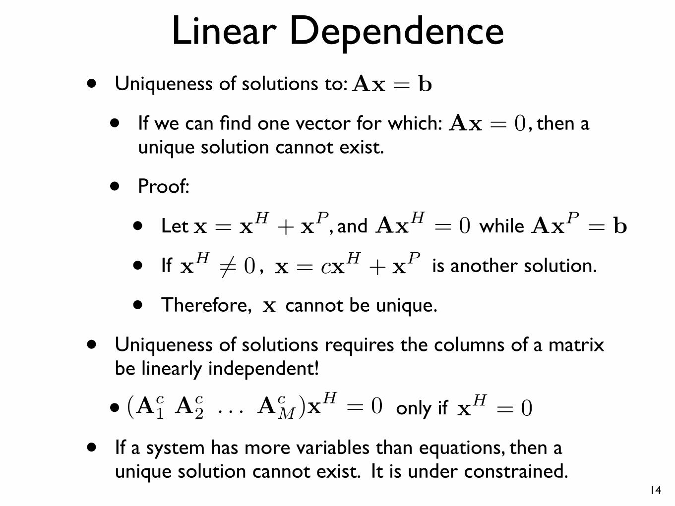
Linear Dependence • Uniqueness of solutions to:

Ax = b

• If we can find one vector for which: Ax = 0 , then a

unique solution cannot exist.

• Proof: H P• Let

x = x + x , and Ax

H = 0 while Ax

P = b H H P• If x 6= 0 ,

x = cx + x is another solution.

• Therefore, x cannot be unique.

• Uniqueness of solutions requires the columns of a matrix be linearly independent!

• (A1 c A2

c . . . AMc )x H = 0 only if

x H = 0

• If a system has more variables than equations, then a unique solution cannot exist. It is under constrained.

14

Linear Dependence

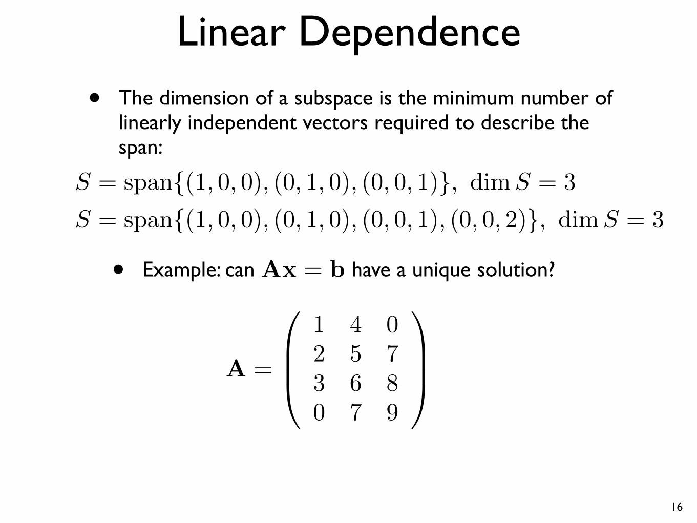
• The dimension of a subspace is the minimum number of linearly independent vectors required to describe the span:

S = span{(1, 0, 0), (0, 1, 0), (0, 0, 1)}, dim S = 3

S = span{(1, 0, 0), (0, 1, 0), (0, 0, 1), (0, 0, 2)}, dim S = 3

• Example: can Ax = b have a unique solution?

0 1 4 0

1

2 5 7 A =

B CB3 6 8

C@ A

0 7 9

15

Linear Dependence

• The dimension of a subspace is the minimum number of linearly independent vectors required to describe the span:

S = span{(1, 0, 0), (0, 1, 0), (0, 0, 1)}, dim S = 3

S = span{(1, 0, 0), (0, 1, 0), (0, 0, 1), (0, 0, 2)}, dim S = 3

• Example: can Ax = b have a unique solution?

0 1 4 0

1

2 5 7 A =

B CB3 6 8

C@ A

0 7 9

16

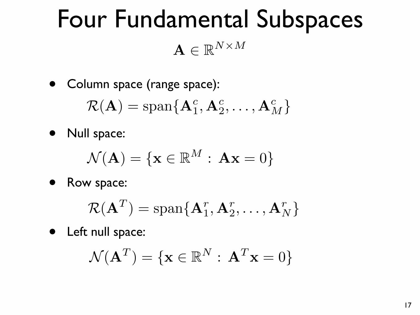
Four Fundamental Subspaces A 2 RN⇥M

• Column space (range space):

R(A) = span{A1,A2, . . . ,AcM

cc }

• Null space:

N (A) = {x 2 RM : Ax = 0}

• Row space:

R(AT ) = span{Ar 1,A2

r , . . . ,Ar N }

• Left null space:

N (AT ) = {x 2 RN : AT x = 0}

17

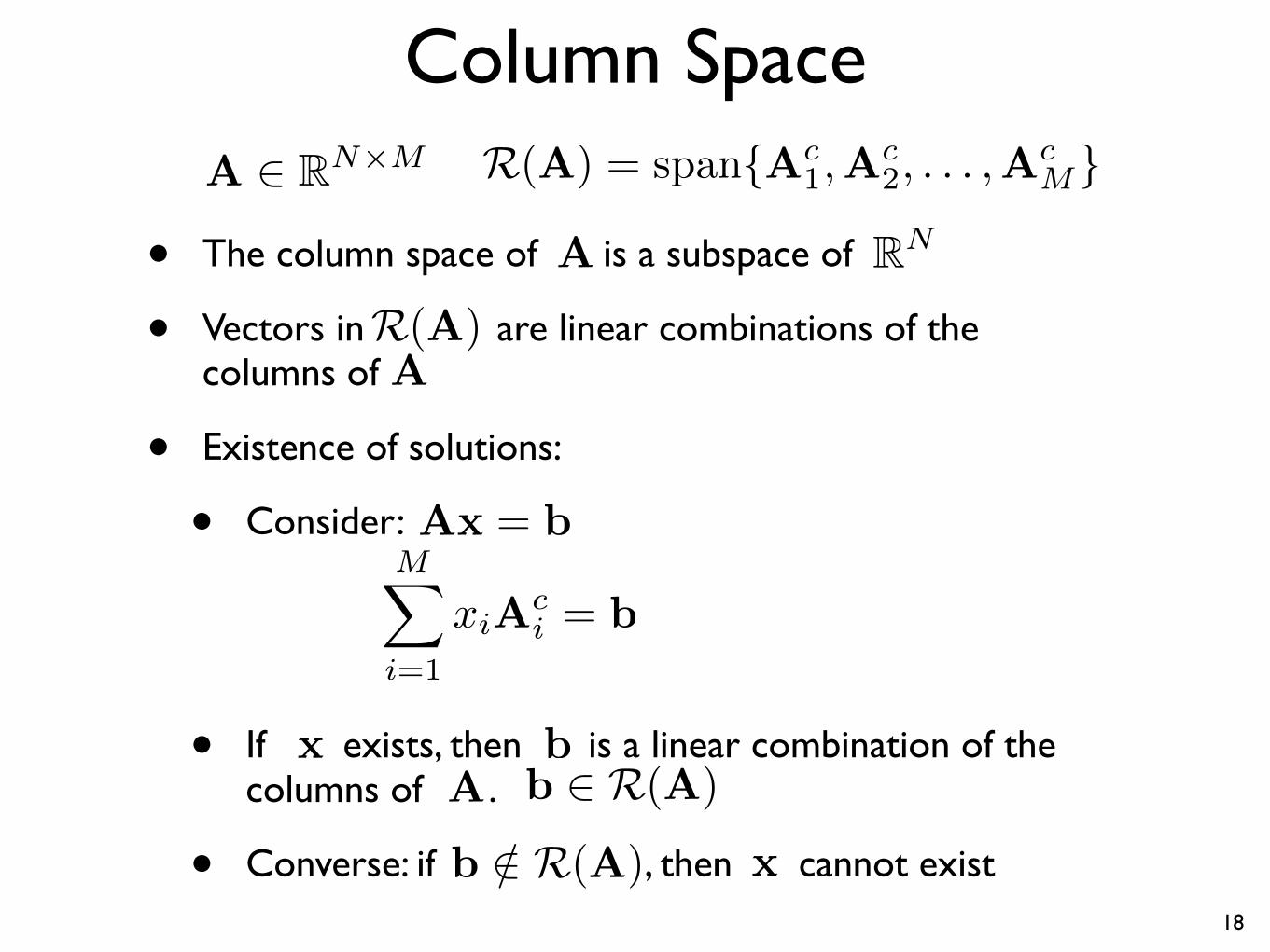
Column Space A 2 RN⇥M R(A) = span{A1,A2, . . . ,A

cM

cc }

• The column space of A is a subspace of RN

• Vectors in R(A) are linear combinations of the columns of A

• Existence of solutions:

• Consider: Ax = b

MX xiA

c = bi i=1

• If x exists, then b is a linear combination of the columns of A. b 2 R(A)

• Converse: if b 2/ R(A), then x cannot exist 18

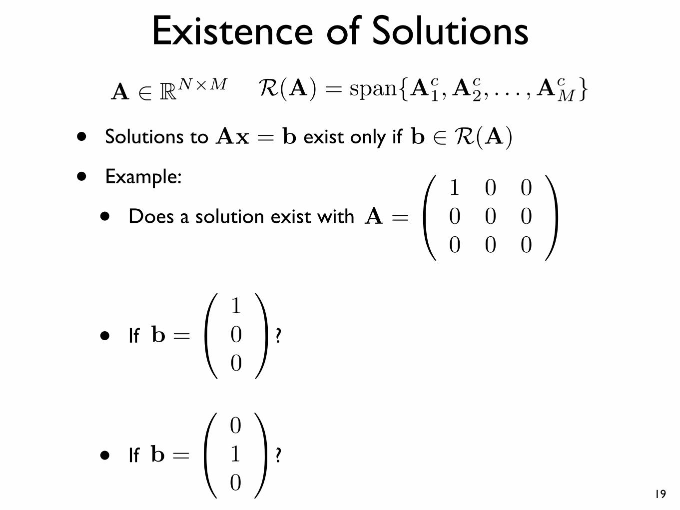
Existence of Solutions A 2 RN⇥M R(A) = span{A1,A2, . . . ,A

cM

cc }

• Solutions to Ax = b exist only if b 2 R(A)

• Example: 0 1 0 0

1

• Does a solution exist with A = 0 0 0 @ A

0 0 0

0 1

1

• If b = 0 ?@ A

0

0 0

1

• If b = 1 ?@ A

0 19

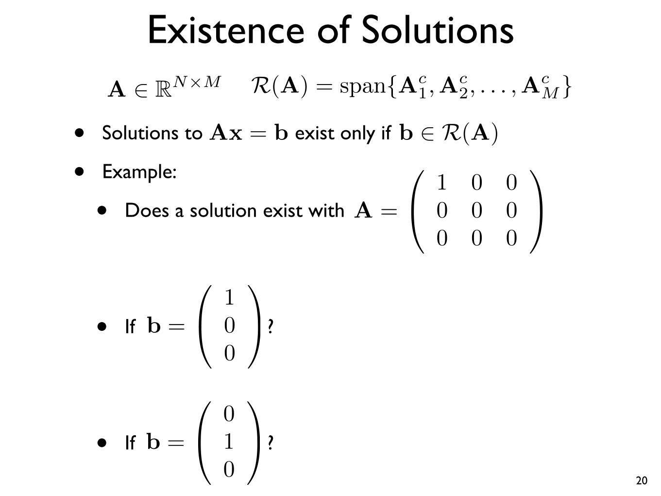
Existence of Solutions A 2 RN⇥M R(A) = span{A1,A2, . . . ,A

cM

cc }

• Solutions to Ax = b exist only if b 2 R(A)

• Example: 0 1 0 0

1

• Does a solution exist with A = 0 0 0 @ A

0 0 0

0 1

1

• If b = 0 ?@ A

0

0 0

1

• If b = 1 ?@ A

0 20

Existence of Solutions

• Does a solution exist?

separator, 2:1 3 kg/s

1.1 kg/s

?

? • Example:

0 1

A ✓

x1◆

= x2

0

@

11 1 3

@ �2 1 1 0

A0 1.1

• What is the column space?

•

21

• Is b 2 R(A) ?

Null Space A 2 RN⇥M

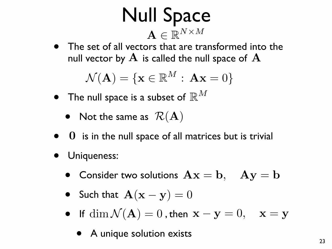
• The set of all vectors that are transformed into the null vector by A is called the null space of A

N (A) = {x 2 RM : Ax = 0}

• The null space is a subset of RM

• Not the same as R(A)

• 0 is in the null space of all matrices but is trivial

• Uniqueness:

• Consider two solutions Ax = b, Ay = b

• Such that A(x � y) = 0

• If dim N (A) = 0 , then x � y = 0, x = y

• A unique solution exists 23

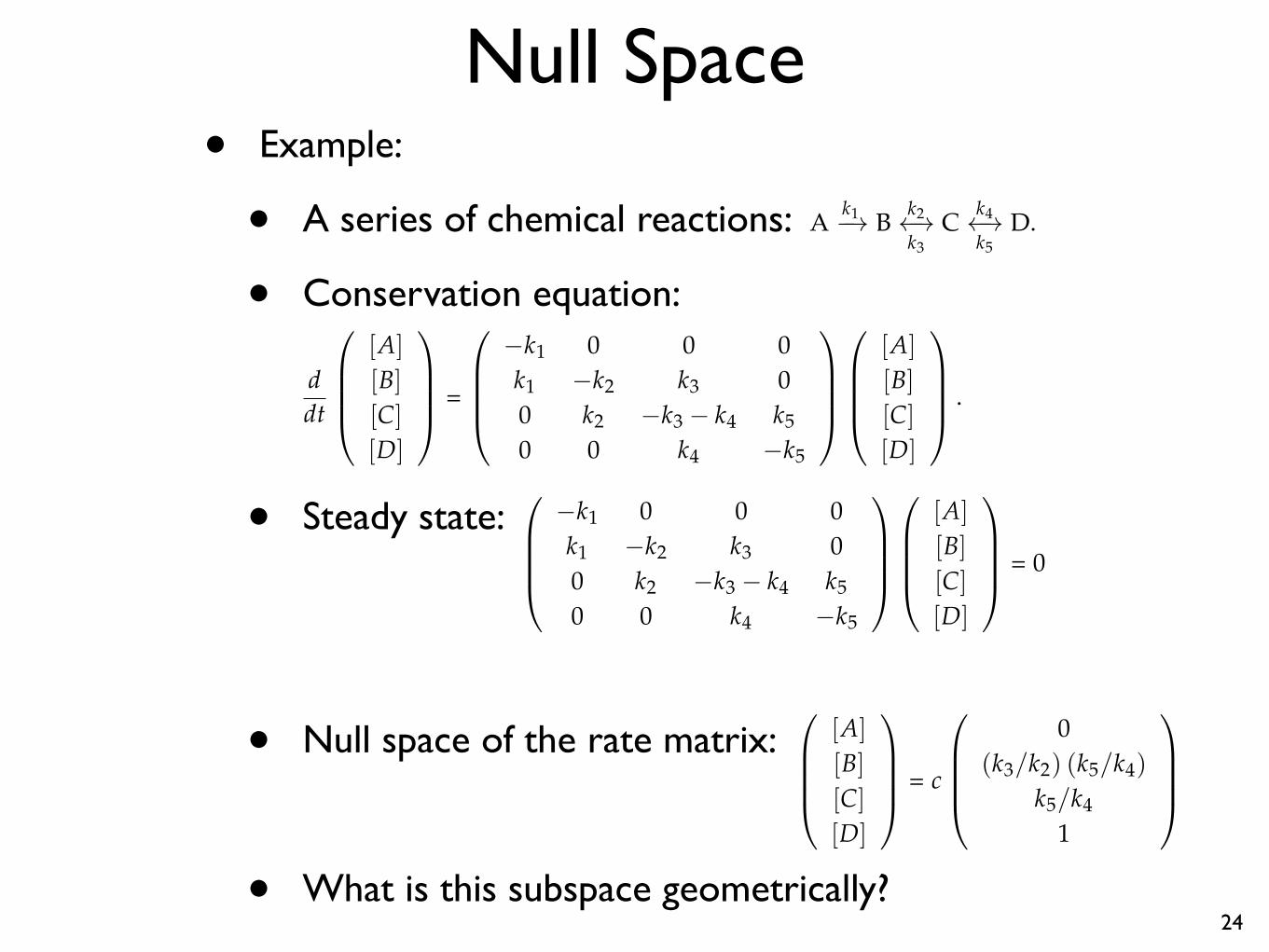
Null Space• Example:

• A series of chemical reactions:

• Conservation equation:

• Steady state:

• Null space of the rate matrix:

• What is this subspace geometrically?24

systems of linear equations 41

• For a matrix in CN⇥N , the secular equation is a polynomial of degreeN. There are N roots and thus N eigenvalues.

• Like the roots of a polynomial, the eigenvalues need not be distinct.The eigenvalues of the identity matrix are all unity, for instance.

• Eigenvalues may be real or complex valued.

• If a matrix belongs to RN⇥N , any complex eigenvalues will appear asconjugate pairs. That is, for each complex eigenvalue, l, its complexconjugate, l̄, is also an eigenvalue.

• For a matrix A 2 CN⇥N , det(A) = l1l2 . . . lN .

• For a matrix A 2 CN⇥N , tr(A) = l1 + l2 + . . . lN .

An example

Consider the reaction network:

Ak1�! B

k2 !k3

Ck4 !k5

D.

If the reaction takes place in a well mixed, batch vessel, then the rate ofchange of concentration of each species is

ddt

0

B

B

B

@

[A]

[B]

[C]

[D]

1

C

C

C

A

=

0

B

B

B

@

�k1 0 0 0k1 �k2 k3 00 k2 �k3 � k4 k5

0 0 k4 �k5

1

C

C

C

A

0

B

B

B

@

[A]

[B]

[C]

[D]

1

C

C

C

A

.

When the reaction reaches its steady-state (d/dt[⇤] = 0), the rate equa-tion is simply:

0

B

B

B

@

�k1 0 0 0k1 �k2 k3 00 k2 �k3 � k4 k5

0 0 k4 �k5

1

C

C

C

A

0

B

B

B

@

[A]

[B]

[C]

[D]

1

C

C

C

A

= 0 or 0

0

B

B

B

@

[A]

[B]

[C]

[D]

1

C

C

C

A

,

There must be a non-trivial solution for the steady concentrations – aneigenvector corresponding to an eigenvalue of zero. The eigenvalues ofthe rate matrix are given by the secular equation:

0 = det

0

B

B

B

@

�k1 � l 0 0 0k1 �k2 � l k3 00 k2 �k3 � k4 � l k5

0 0 k4 �k5 � l

1

C

C

C

A

(2.52)

= l(l + k1)h

l

2 + (k2 + k3 + k4 + k4) l + k2k4 + k2k5 + k3k5

i

,

which has the obvious roots l = 0 and l = �k1 as well as two otherroots. Therefore l = 0 is indeed a root. Because the determinant of








An example


Ak1�! B

k2 !k3

Ck4 !k5

D.


ddt

0

B

B

B

@

[A]

[B]

[C]

[D]

1

C

C

C

A

=

0

B

B

B

@

�k1 0 0 0k1 �k2 k3 00 k2 �k3 � k4 k5

0 0 k4 �k5

1

C

C

C

A

0

B

B

B

@

[A]

[B]

[C]

[D]

1

C

C

C

A

.


0

B

B

B

@

�k1 0 0 0k1 �k2 k3 00 k2 �k3 � k4 k5

0 0 k4 �k5

1

C

C

C

A

0

B

B

B

@

[A]

[B]

[C]

[D]

1

C

C

C

A

= 0 or 0

0

B

B

B

@

[A]

[B]

[C]

[D]

1

C

C

C

A

,


0 = det

0

B

B

B

@

�k1 � l 0 0 0k1 �k2 � l k3 00 k2 �k3 � k4 � l k5

0 0 k4 �k5 � l

1

C

C

C

A

(2.52)

= l(l + k1)h

l

2 + (k2 + k3 + k4 + k4) l + k2k4 + k2k5 + k3k5

i

,









An example


Ak1�! B

k2 !k3

Ck4 !k5

D.


ddt

0

B

B

B

@

[A]

[B]

[C]

[D]

1

C

C

C

A

=

0

B

B

B

@

�k1 0 0 0k1 �k2 k3 00 k2 �k3 � k4 k5

0 0 k4 �k5

1

C

C

C

A

0

B

B

B

@

[A]

[B]

[C]

[D]

1

C

C

C

A

.


0

B

B

B

@

�k1 0 0 0k1 �k2 k3 00 k2 �k3 � k4 k5

0 0 k4 �k5

1

C

C

C

A

0

B

B

B

@

[A]

[B]

[C]

[D]

1

C

C

C

A

= 0

0

B

B

B

@

[A]

[B]

[C]

[D]

1

C

C

C

A

,


0 = det

0

B

B

B

@

�k1 � l 0 0 0k1 �k2 � l k3 00 k2 �k3 � k4 � l k5

0 0 k4 �k5 � l

1

C

C

C

A

(2.52)

= l(l + k1)h

l

2 + (k2 + k3 + k4 + k4) l + k2k4 + k2k5 + k3k5

i

,


42 10.34: numerical methods, lecture notes

a matrix is equal to a product of its eigenvalues, the rate matrix issingular. Physically, this must be the case since conservation of totalmass relates individual species rate equations. They are not linearlyindependent.

To the eigenvalue of zero, there is a corresponding eigenvector thatdescribes the chemical engineer’s intuition: at steady state, [A] = 0as it is depleted by only forward reactions, while [B], [C] and [D]obtain non-zero values set by the equilibrium of the reactions betweenthese species. This eigenvector is a set of non-zero concentrations thatbelongs to the null space of the reaction rate matrix. This set may bedetermined by assuming [D] = 1 and performing back substitution todetermine the concentrations of the other components. The family ofnon-zero vectors satisfying steady-state condition is

0

B

B

B

@

[A]

[B]

[C]

[D]

1

C

C

C

A

= c

0

B

B

B

@

0(k3/k2) (k5/k4)

k5/k41

1

C

C

C

A

. (2.53)

where c is an arbitrary scalar that is determined by a total mole bal-ance on the steady-state. Because the stoichiometric relationshipsbetween the components of the network is 1, the final number ofmoles in the vessel must match the initial number. Equivalently,c[0 + (k3/k2)(k5/k4) + (k5/k4) + 1] = N0/V, where N0 is the initial num-ber of moles in the vessel and V is the vessel’s volume. Thus,

c =N0

V[1 + (k5/k4)(1 + k3/k2)].

2.5.1 Eigenvalue decomposition

For an eigenvalue li of a matrix A 2 CN⇥N , the null space of A� liI

isN (A� liI) =

n

wi 2 CN : (A� liI)wi = 0o

. (2.54)

This null space is also called the “eigenspace” for li. It spans theeigenvectors associated with this eigenvalue. If li is a distinct root ofthe secular equation, then dim N (A� liI) = 1. If li is a multiple root:

p(l) = . . . (l � li)m . . . = 0, (2.55)

it is said to have algebraic multiplicity m. The dimension of N (A �liI) is termed the geometric multiplicity and reflects the number oflinearly independent eigenvectors associated with this eigenvalue. Thegeometric multiplicity is always greater than zero and less than m + 1.When the two coincide for all of the eigenvalues of A, the matrix issaid to have a complete set of linearly independent eigenvectors.

38 10.34: numerical methods, lecture notes

Matrix rank

The rank of a matrix, A 2 CN⇥M, is denoted r and defined as thedimension of its column space:

r = dim R(A). (2.46)

The dimension of the null space is necessarily r � M:

dim N (A) = r � M.

If the rank of a matrix equals the number of columns in the matrix,r = M, the dimension of the null space is zero. Such a matrix is saidto be full rank. The rank of a matrix can be determined by reducing itto row-echelon form: A ! U . This is done by following the Gaussianelimination procedure with pivoting. The row-echelon form matrix, U ,will have the structure:

. (2.47)

A square, non-singular matrix in CN⇥N , has rank r = N. The matrixis singular if r < N – the columns of the matrix are linearly dependent.A matrix in CN⇥M is termed rank deficient if r min(N, M). Likewise,when r < M, solutions, if any exist, are not unique.

Row space and left null space

The row space of a matrix A 2 CN⇥M is defined as the column spaceof AT : R(AT). If A has rank r, the dimension of the row space of Ais also r. The left null space of A is the null space of AT : N (AT). Thedimension of the left null space is N � r. Note that

R(AT) ⇢ CM ,

andN (AT) ⇢ CN .

The column space and left null space of A are subsets of the samevector space CN .

The column space and left null space are termed orthogonal compli-ments. Likewise, the row space and null space of A are subsets of CM

and are also orthogonal compliments. The orthogonal compliment of asubset S is a subset S?. By definition, every vector v 2 S is orthogonalto every vector v? 2 S?: v · v? = 0.

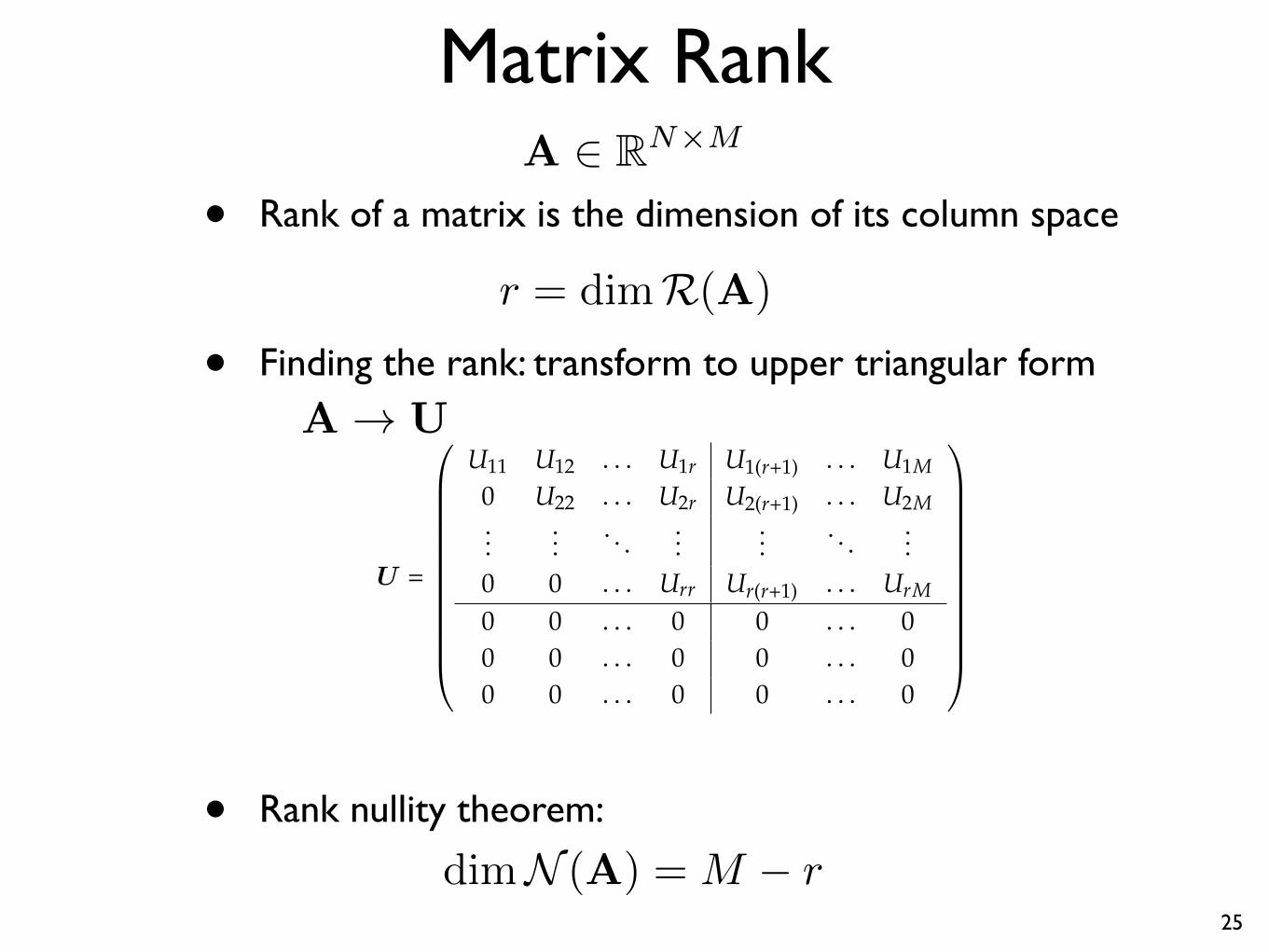
Matrix Rank A 2 RN⇥M

• Rank of a matrix is the dimension of its column space

r = dimR(A)

• Finding the rank: transform to upper triangular form A ! U

0

B

B

B

B

B

B

B

B

B

B

B

@

U11 U12 . . . U1r U1(r+1) . . . U1M

0 U22 . . . U2r U2(r+1) . . . U2M . . .

. . . . . .

. . . . . .

. . . . . .

U =

1

C

C

C

C

C

C

C

C

C

C

C

A

0

0

0

0

. . .

. . .

Urr

0

Ur(r+1)

0

. . .

. . .

UrM

0

0 0 . . . 0 0 . . . 0

0 0 . . . 0 0 . . . 0

• Rank nullity theorem:

dim N (A) = M � r 25

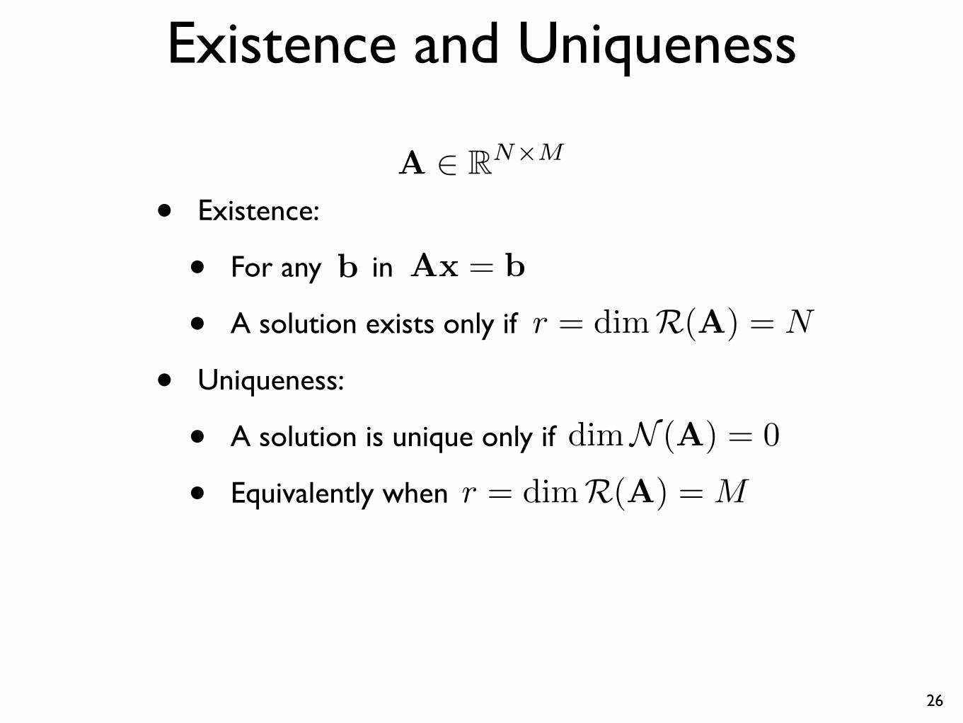
Existence and Uniqueness

A 2 RN⇥M

• Existence:

• For any b in Ax = b

• A solution exists only if r = dimR(A) = N

• Uniqueness:

• A solution is unique only if dim N (A) = 0

• Equivalently when r = dimR(A) = M

26

MIT OpenCourseWarehttps://ocw.mit.edu

10.34 Numerical Methods Applied to Chemical EngineeringFall 2015

For information about citing these materials or our Terms of Use, visit: https://ocw.mit.edu/terms.

https://ocw.mit.edu

https://ocw.mit.edu/terms

Documents

10.34: Numerical Methods Applied to Chemical Engineering