Embed Size (px)
Citation preview
04/20/23 COSC-3308-01, Lecture 10 1
Programming Language Concepts, COSC-3308-01Lecture 10
Relational ProgrammingConstraints programming
04/20/23 COSC-3308-01, Lecture 10 2
Reminder of the Last Lecture Introduction to Stateful Programming: what is state? Stateful programming
cells as abstract datatypes the stateful model relationship between the declarative model and the stateful
model indexed collections:
array model ports
system building component-based programming
Object-oriented programming Classes
04/20/23 COSC-3308-01, Lecture 10 3
Overview Relational programming
Choice and Fail Operations Constraints Programming
Basic Constraints, Propagators and Search
04/20/23 COSC-3308-01, Lecture 10 4
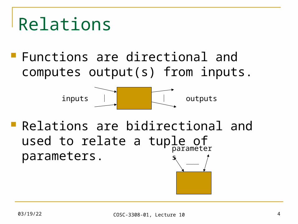
Relations
Functions are directional and computes output(s) from inputs.
Relations are bidirectional and used to relate a tuple of parameters.
inputs outputs
parameters
04/20/23 COSC-3308-01, Lecture 10 5
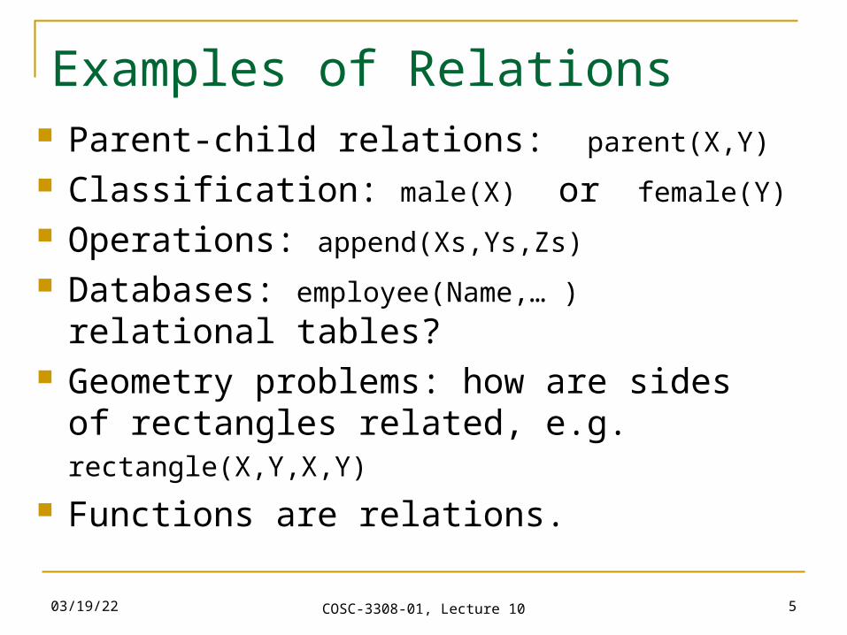
Examples of Relations Parent-child relations: parent(X,Y) Classification: male(X) or female(Y) Operations: append(Xs,Ys,Zs) Databases: employee(Name,… ) relational
tables? Geometry problems: how are sides of
rectangles related, e.g. rectangle(X,Y,X,Y) Functions are relations.
04/20/23 COSC-3308-01, Lecture 10 6
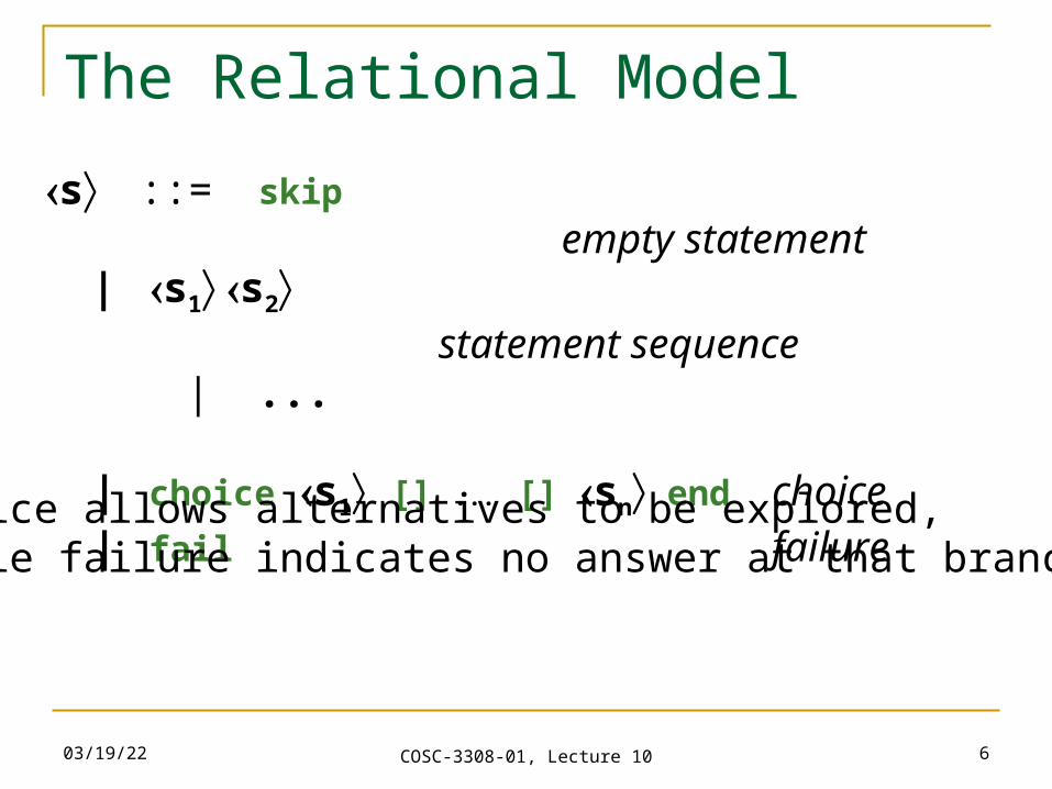
The Relational Model
s::= skip empty statement| s1 s2 statement sequence
| ... | choice s1 [] ... [] sn end choice| fail failure
Choice allows alternatives to be explored, while failure indicates no answer at that branch.
04/20/23 COSC-3308-01, Lecture 10 7
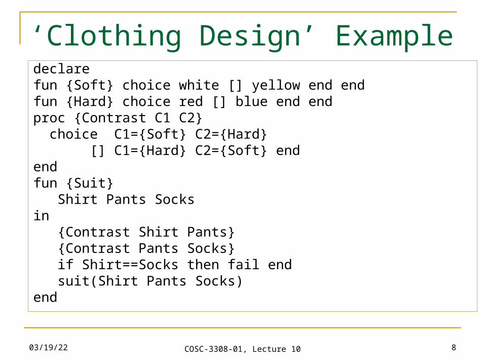
‘Clothing Design’ Example
Goal: help the clothing designer pick colors for a man’s casual suit.
A man’s casual suit is made of: Shirt Pants Socks
Constraints for the choices: Adjacent garments are in contrasting colors; Shirt and socks are of different colors.
04/20/23 COSC-3308-01, Lecture 10 8
‘Clothing Design’ Exampledeclarefun {Soft} choice white [] yellow end endfun {Hard} choice red [] blue end endproc {Contrast C1 C2} choice C1={Soft} C2={Hard} [] C1={Hard} C2={Soft} endendfun {Suit} Shirt Pants Socks in {Contrast Shirt Pants} {Contrast Pants Socks} if Shirt==Socks then fail end suit(Shirt Pants Socks)end
04/20/23 COSC-3308-01, Lecture 10 9
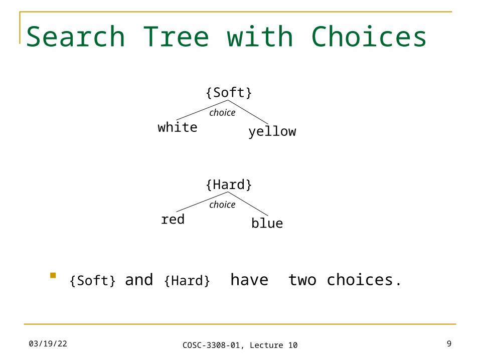
Search Tree with Choices
{Soft}
white yellowchoice
{Hard}
red bluechoice
{Soft} and {Hard} have two choices.
04/20/23 COSC-3308-01, Lecture 10 10
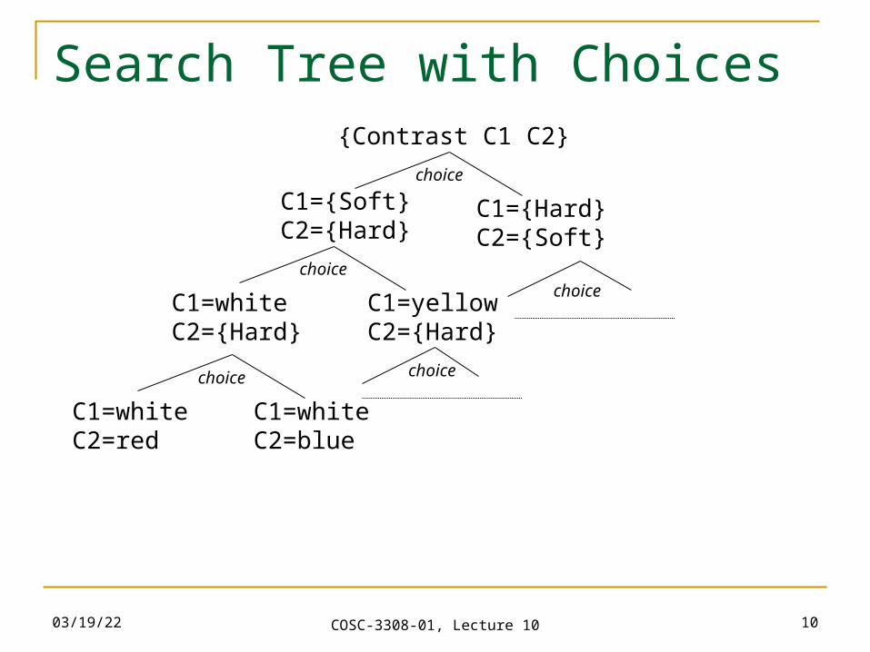
Search Tree with Choices{Contrast C1 C2}
C1={Soft}C2={Hard}
choice
C1={Hard}C2={Soft}
C1=whiteC2={Hard}
C1=yellowC2={Hard}
choice
C1=whiteC2=red
C1=whiteC2=blue
choice choice
choice
04/20/23 COSC-3308-01, Lecture 10 11
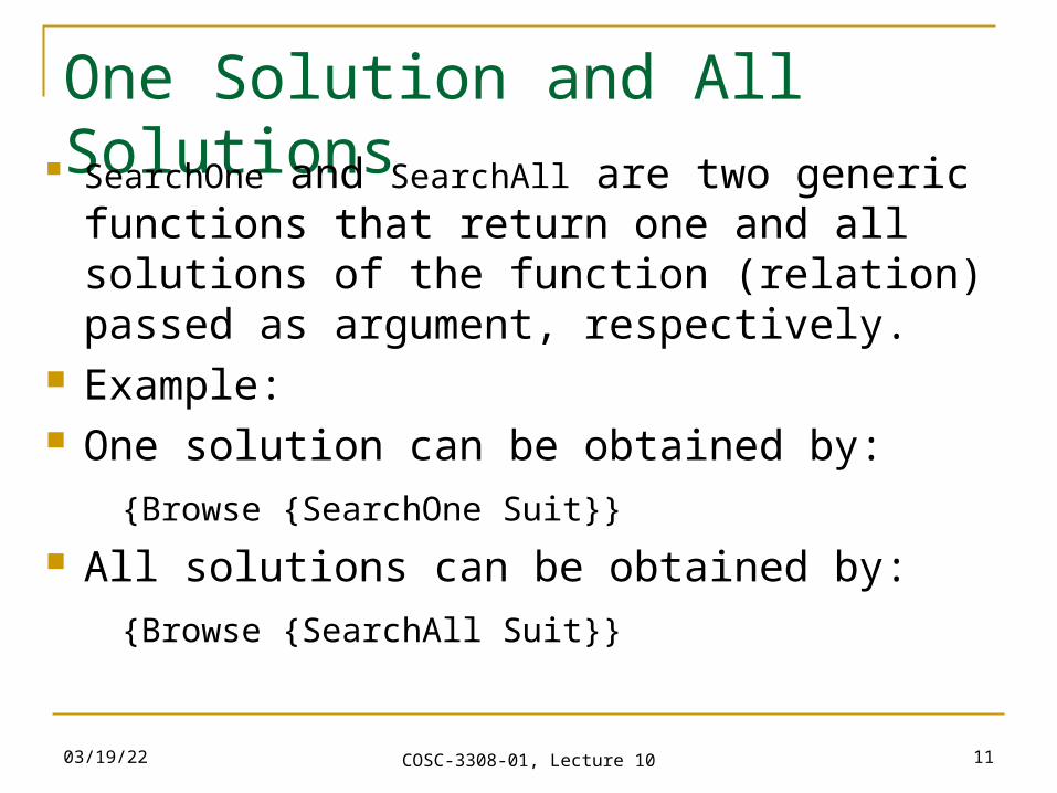
One Solution and All Solutions SearchOne and SearchAll are two generic functions that return one and all solutions of the function (relation) passed as argument, respectively.
Example: One solution can be obtained by:
{Browse {SearchOne Suit}} All solutions can be obtained by:
{Browse {SearchAll Suit}}
04/20/23 COSC-3308-01, Lecture 10 12
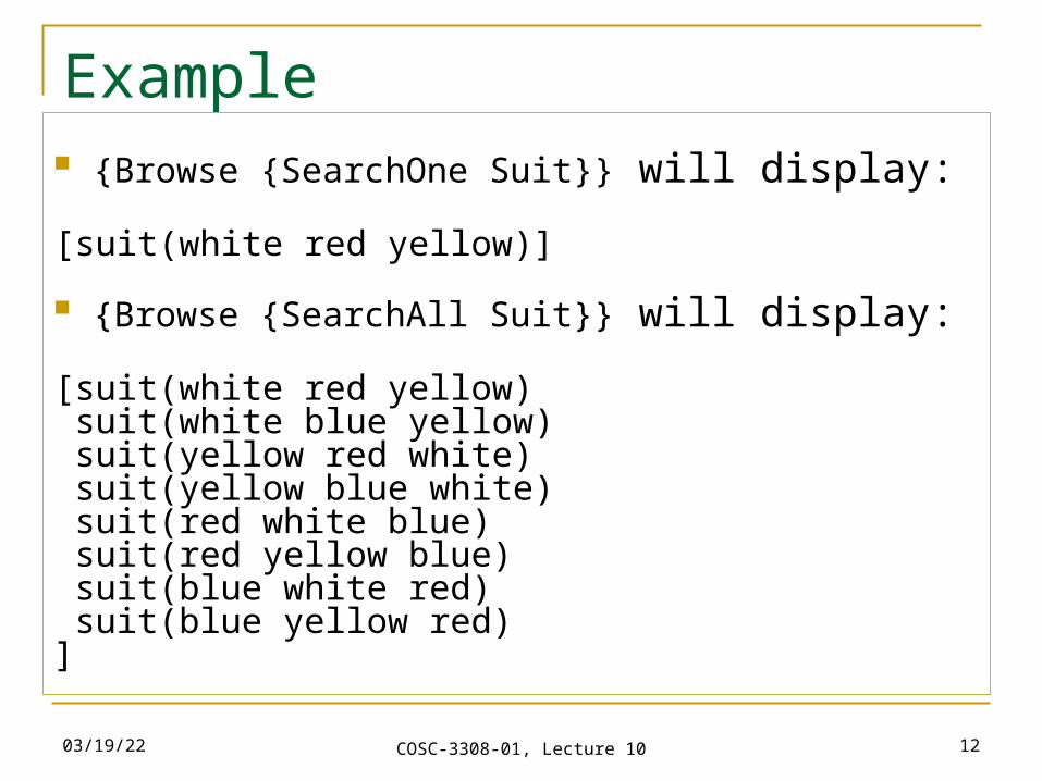
Example {Browse {SearchOne Suit}} will display:
[suit(white red yellow)]
{Browse {SearchAll Suit}} will display:
[suit(white red yellow) suit(white blue yellow) suit(yellow red white) suit(yellow blue white) suit(red white blue) suit(red yellow blue) suit(blue white red) suit(blue yellow red)]
04/20/23 COSC-3308-01, Lecture 10 13
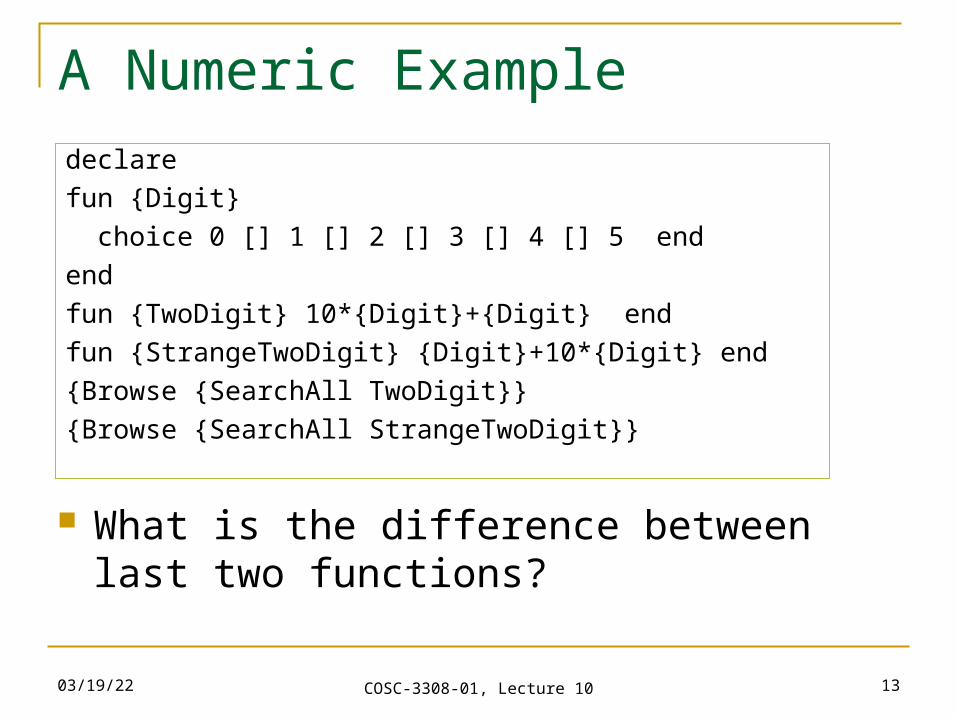
A Numeric Exampledeclare
fun {Digit}
choice 0 [] 1 [] 2 [] 3 [] 4 [] 5 end
end
fun {TwoDigit} 10*{Digit}+{Digit} end
fun {StrangeTwoDigit} {Digit}+10*{Digit} end
{Browse {SearchAll TwoDigit}}
{Browse {SearchAll StrangeTwoDigit}}
What is the difference between last two functions?
04/20/23 COSC-3308-01, Lecture 10 14
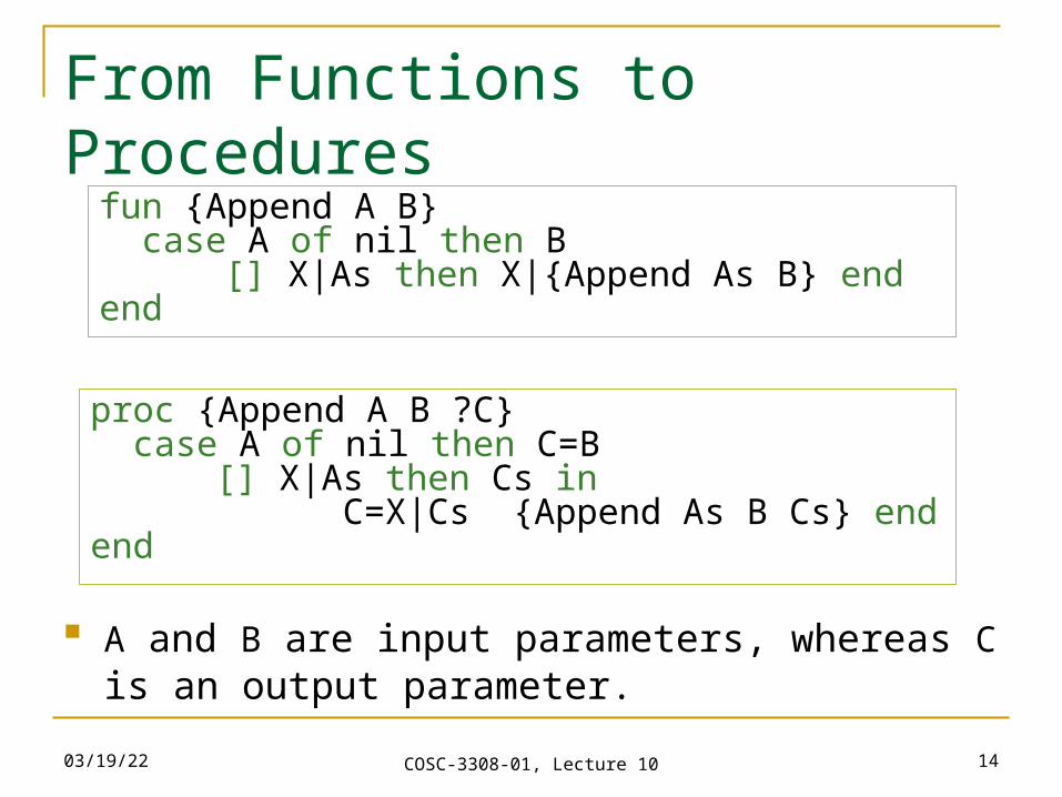
From Functions to Proceduresfun {Append A B} case A of nil then B [] X|As then X|{Append As B} end
end
proc {Append A B ?C} case A of nil then C=B [] X|As then Cs in
C=X|Cs {Append As B Cs} endend
A and B are input parameters, whereas C is an output parameter.
04/20/23 COSC-3308-01, Lecture 10 15
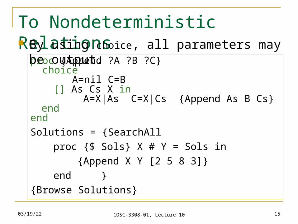
To Nondeterministic Relations
proc {Append ?A ?B ?C} choice A=nil C=B [] As Cs X in
A=X|As C=X|Cs {Append As B Cs} end
end
Solutions = {SearchAll
proc {$ Sols} X # Y = Sols in
{Append X Y [2 5 8 3]}
end }
{Browse Solutions}
By using choice, all parameters may be output.
04/20/23 COSC-3308-01, Lecture 10 16
Constraint Programming
Ultimate in declarative modelling. Here, we focus on Finite Domain Constraint
Programming CP(FD); CP initially conceived as framework CLP(X) [Jaffar, Lassez; 1987]
Within CP(FD), we focus on constraint-based tree search.
04/20/23 COSC-3308-01, Lecture 10 17
Definitions and Notations I
Finite domain: is a finite set of nonnegative integers. The notation m#n stands for the finite domain m...n.
Constraints over finite domains: is a formula of predicate logic. Examples:
X=5 X1#9 X2-Y2=Z2
04/20/23 COSC-3308-01, Lecture 10 18
Definitions and Notations II Domain constraint:
takes the form XD, where D is a finite domain. Domain constraints can express constraints of the form X=n, being equivalent to Xn#n.
Basic constraint: takes one of the following forms: X=n, X=Y, or XD,
where D is a finite domain. Finite domain constraint problem:
is a finite set P of quantifier-free constraints such that P contains a domain constraint for every variable occurring in a constraint of P.
04/20/23 COSC-3308-01, Lecture 10 19
Definitions and Notations III A typical finite domain constraint problem or
constraint satisfaction problem (CSP) consists of: Input:
number of variables: n constraints: c1,…,cm
n
Goal: find a = (v1,…,vn) n such that a ci, for all 1 i m
Variable assignment: is a function mapping variables to integers.
Solution of a finite domain constraints problem P: is a variable assignment that satisfies every constraint in P.
04/20/23 COSC-3308-01, Lecture 10 20
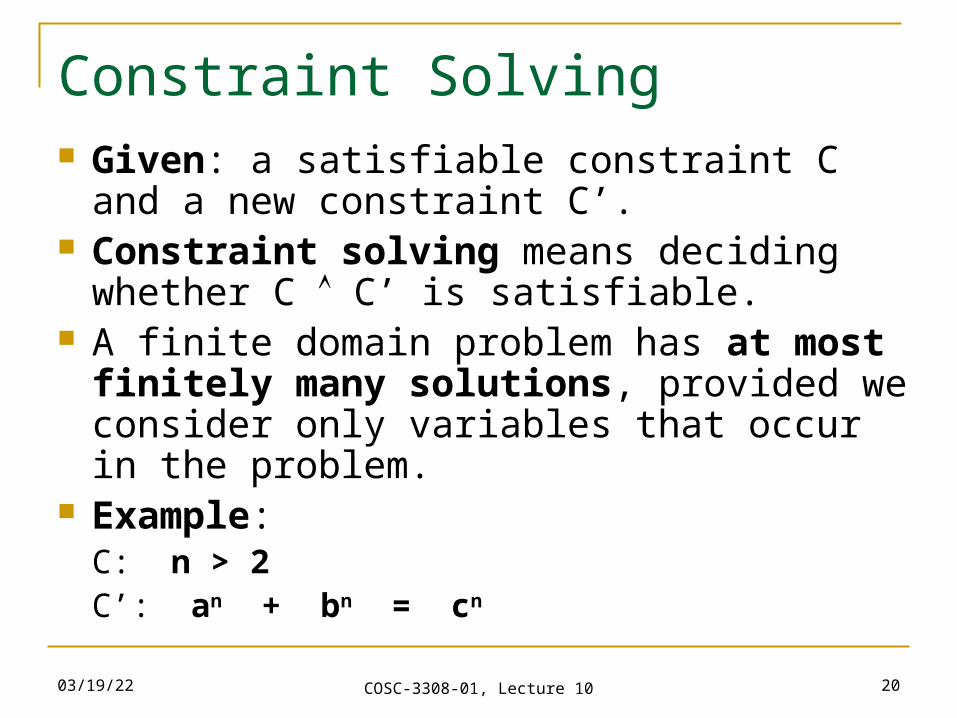
Constraint Solving Given: a satisfiable constraint C and a new
constraint C’. Constraint solving means deciding whether
C C’ is satisfiable. A finite domain problem has at most finitely
many solutions, provided we consider only variables that occur in the problem.
Example: C: n > 2C’: an + bn = cn
04/20/23 COSC-3308-01, Lecture 10 21
Constraint Solving
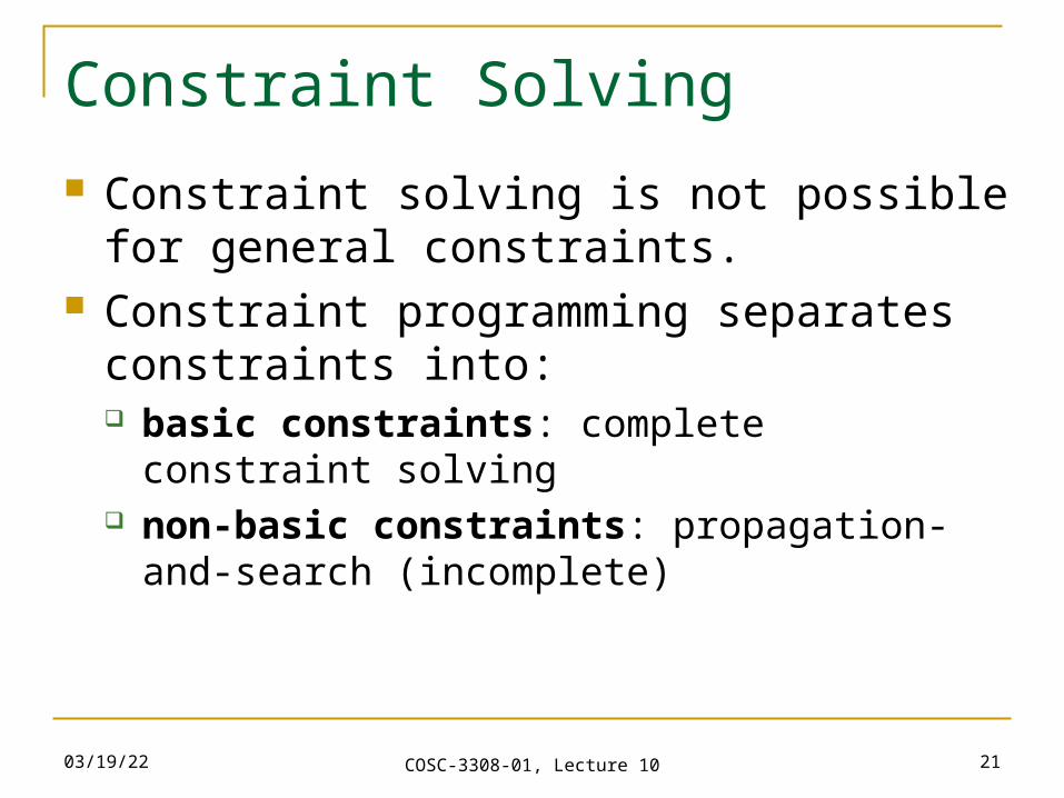
Constraint solving is not possible for general constraints.
Constraint programming separates constraints into: basic constraints: complete constraint solving non-basic constraints: propagation-and-search
(incomplete)
04/20/23 COSC-3308-01, Lecture 10 22
Basic Constraints in Finite Domain Constraint Programming
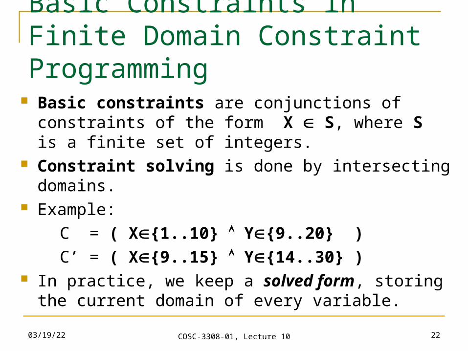
Basic constraints are conjunctions of constraints of the form X S, where S is a finite set of integers.
Constraint solving is done by intersecting domains. Example:
C = ( X{1..10} Y{9..20} ) C’ = ( X{9..15} Y{14..30} ) In practice, we keep a solved form, storing the current
domain of every variable.
04/20/23 COSC-3308-01, Lecture 10 23
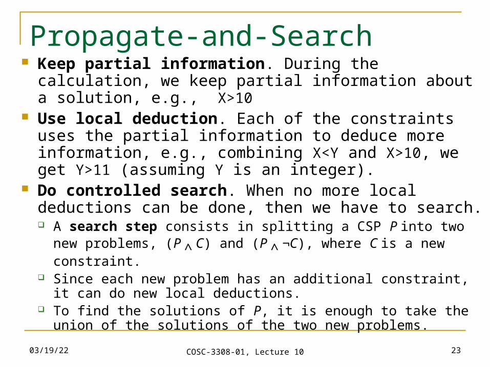
Propagate-and-Search Keep partial information. During the calculation, we
keep partial information about a solution, e.g., X>10 Use local deduction. Each of the constraints uses the
partial information to deduce more information, e.g., combining X<Y and X>10, we get Y>11 (assuming Y is an integer).
Do controlled search. When no more local deductions can be done, then we have to search. A search step consists in splitting a CSP P into two new
problems, (P ^ C) and (P ^ ¬C), where C is a new constraint. Since each new problem has an additional constraint, it can do
new local deductions. To find the solutions of P, it is enough to take the union of the
solutions of the two new problems.
04/20/23 COSC-3308-01, Lecture 10 24
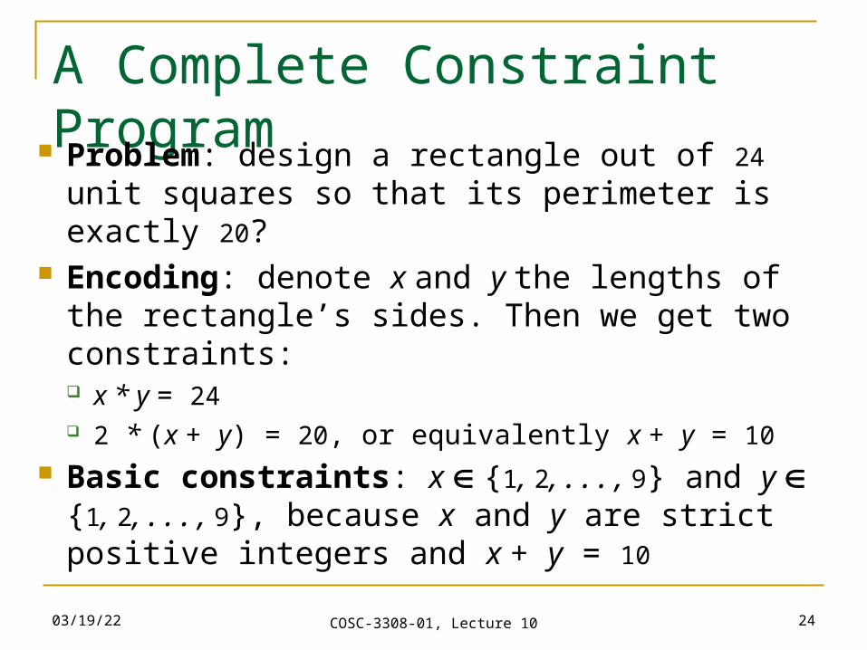
A Complete Constraint Program Problem: design a rectangle out of 24 unit squares so that its perimeter is exactly 20?
Encoding: denote x and y the lengths of the rectangle’s sides. Then we get two constraints: x * y = 24 2 * (x + y) = 20, or equivalently x + y = 10
Basic constraints: x {1, 2, . . . , 9} and y {1, 2, . . . , 9}, because x and y are strict positive integers and x + y = 10
04/20/23 COSC-3308-01, Lecture 10 25
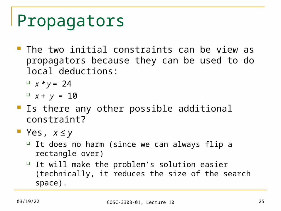
Propagators
The two initial constraints can be view as propagators because they can be used to do local deductions: x * y = 24 x + y = 10
Is there any other possible additional constraint? Yes, x ≤ y
It does no harm (since we can always flip a rectangle over) It will make the problem’s solution easier (technically, it
reduces the size of the search space).
04/20/23 COSC-3308-01, Lecture 10 26
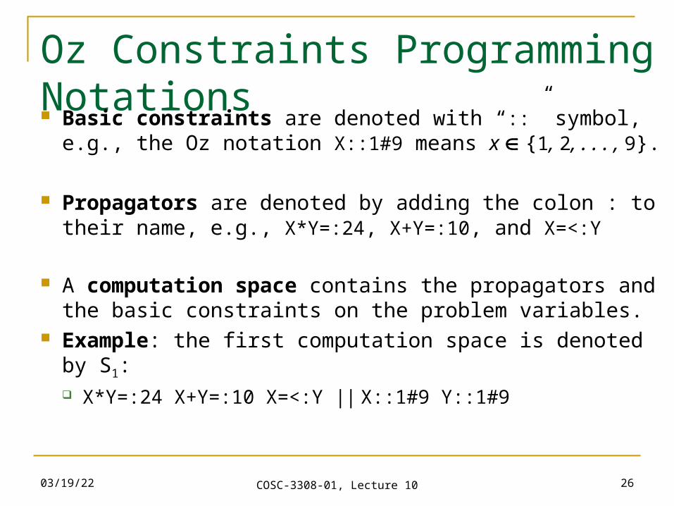
Oz Constraints Programming Notations Basic constraints are denoted with “::” symbol, e.g.,
the Oz notation X::1#9 means x {1, 2, . . . , 9}.
Propagators are denoted by adding the colon : to their name, e.g., X*Y=:24, X+Y=:10, and X=<:Y
A computation space contains the propagators and the basic constraints on the problem variables.
Example: the first computation space is denoted by S1: X*Y=:24 X+Y=:10 X=<:Y || X::1#9 Y::1#9
04/20/23 COSC-3308-01, Lecture 10 27
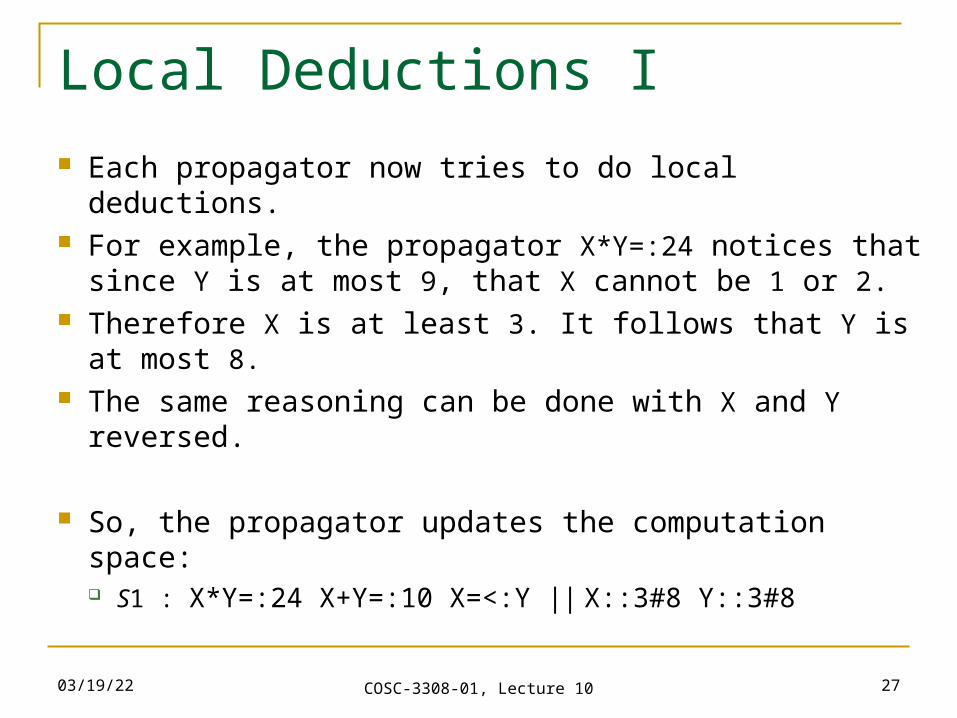
Local Deductions I
Each propagator now tries to do local deductions. For example, the propagator X*Y=:24 notices that
since Y is at most 9, that X cannot be 1 or 2. Therefore X is at least 3. It follows that Y is at most 8. The same reasoning can be done with X and Y
reversed.
So, the propagator updates the computation space: S1 : X*Y=:24 X+Y=:10 X=<:Y || X::3#8 Y::3#8
04/20/23 COSC-3308-01, Lecture 10 28
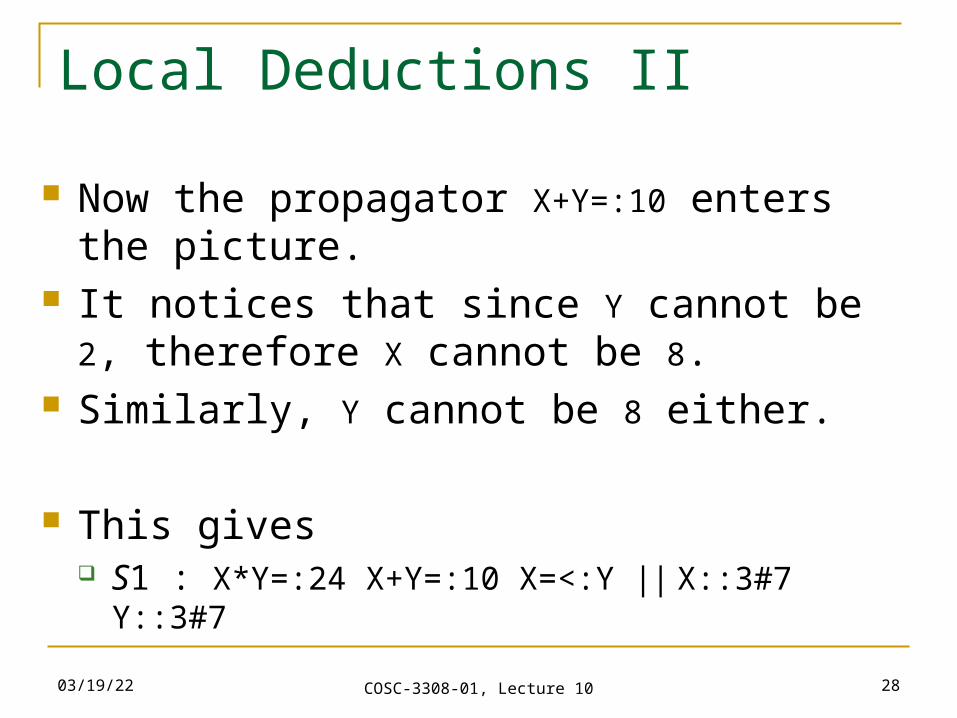
Local Deductions II
Now the propagator X+Y=:10 enters the picture. It notices that since Y cannot be 2, therefore X
cannot be 8. Similarly, Y cannot be 8 either.
This gives S1 : X*Y=:24 X+Y=:10 X=<:Y || X::3#7 Y::3#7
04/20/23 COSC-3308-01, Lecture 10 29
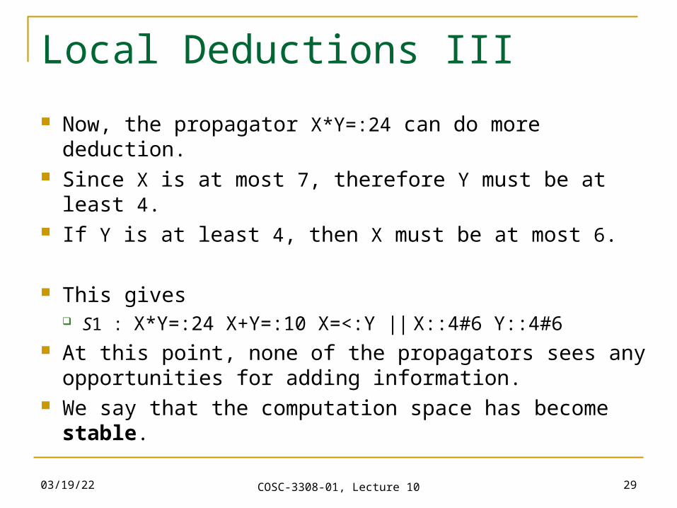
Local Deductions III
Now, the propagator X*Y=:24 can do more deduction. Since X is at most 7, therefore Y must be at least 4. If Y is at least 4, then X must be at most 6.
This gives S1 : X*Y=:24 X+Y=:10 X=<:Y || X::4#6 Y::4#6
At this point, none of the propagators sees any opportunities for adding information.
We say that the computation space has become stable.
04/20/23 COSC-3308-01, Lecture 10 30
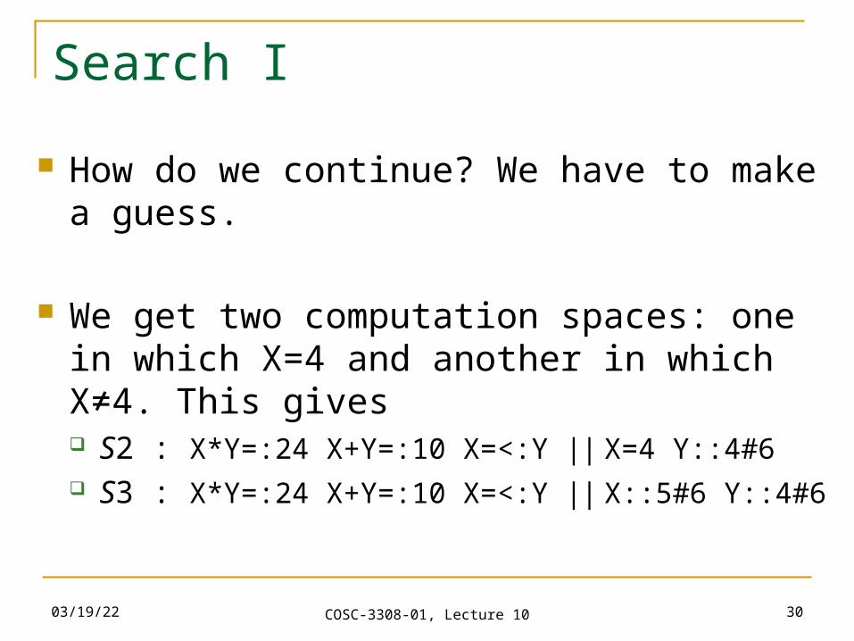
Search I
How do we continue? We have to make a guess.
We get two computation spaces: one in which X=4 and another in which X≠4. This gives S2 : X*Y=:24 X+Y=:10 X=<:Y || X=4 Y::4#6 S3 : X*Y=:24 X+Y=:10 X=<:Y || X::5#6 Y::4#6
04/20/23 COSC-3308-01, Lecture 10 31
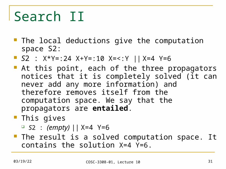
Search II
The local deductions give the computation space S2: S2 : X*Y=:24 X+Y=:10 X=<:Y || X=4 Y=6 At this point, each of the three propagators notices
that it is completely solved (it can never add any more information) and therefore removes itself from the computation space. We say that the propagators are entailed.
This gives S2 : (empty) || X=4 Y=6
The result is a solved computation space. It contains the solution X=4 Y=6.
04/20/23 COSC-3308-01, Lecture 10 32
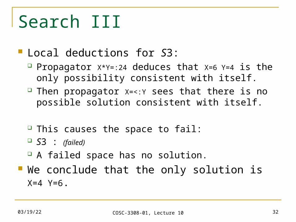
Search III
Local deductions for S3: Propagator X*Y=:24 deduces that X=6 Y=4 is the
only possibility consistent with itself. Then propagator X=<:Y sees that there is no
possible solution consistent with itself.
This causes the space to fail: S3 : (failed) A failed space has no solution.
We conclude that the only solution is X=4 Y=6.
04/20/23 COSC-3308-01, Lecture 10 33
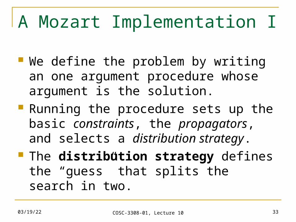
A Mozart Implementation I
We define the problem by writing an one argument procedure whose argument is the solution.
Running the procedure sets up the basic constraints, the propagators, and selects a distribution strategy.
The distribution strategy defines the “guess” that splits the search in two.
04/20/23 COSC-3308-01, Lecture 10 34
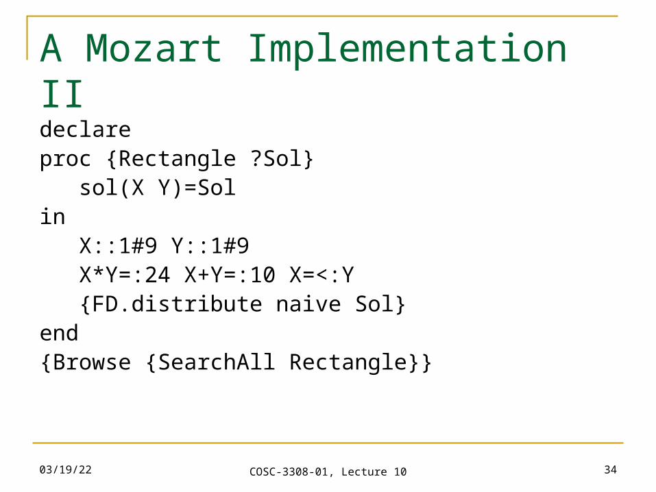
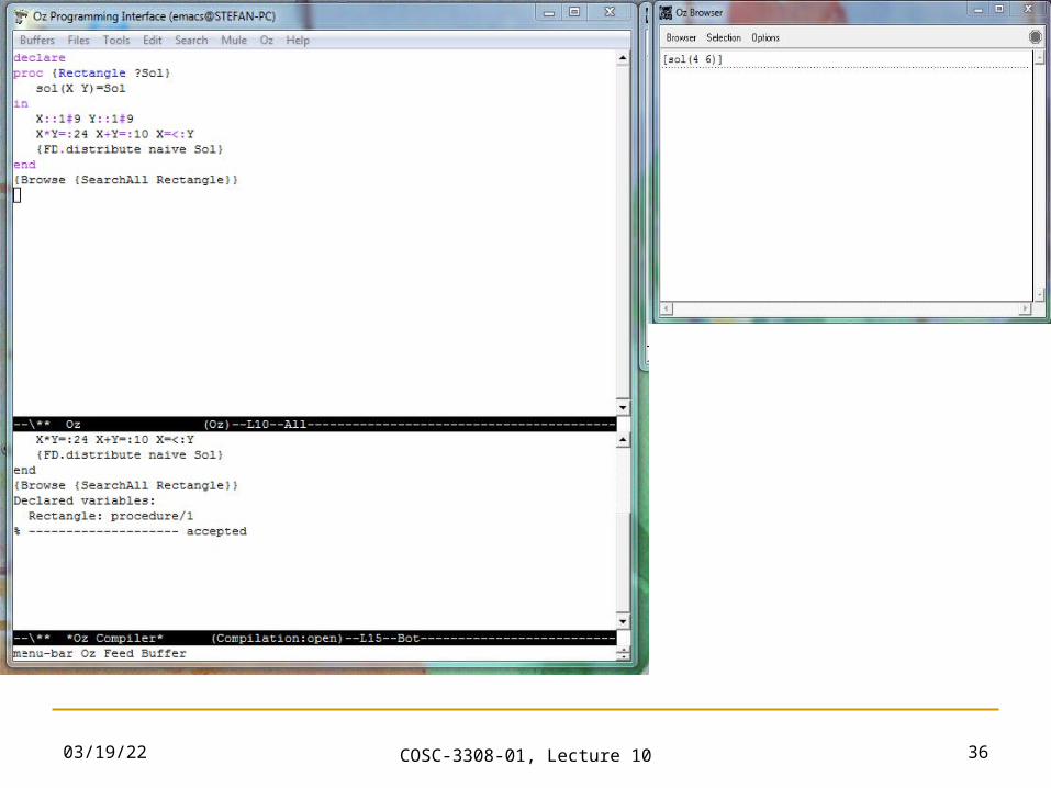
A Mozart Implementation II
declareproc {Rectangle ?Sol} sol(X Y)=Solin X::1#9 Y::1#9 X*Y=:24 X+Y=:10 X=<:Y {FD.distribute naive Sol}end{Browse {SearchAll Rectangle}}
04/20/23 COSC-3308-01, Lecture 10 35
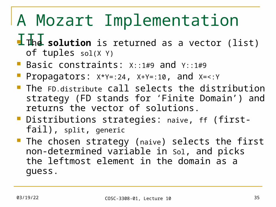
A Mozart Implementation III The solution is returned as a vector (list) of tuples
sol(X Y) Basic constraints: X::1#9 and Y::1#9 Propagators: X*Y=:24, X+Y=:10, and X=<:Y The FD.distribute call selects the distribution strategy
(FD stands for ‘Finite Domain’) and returns the vector of solutions.
Distributions strategies: naive, ff (first-fail), split, generic
The chosen strategy (naive) selects the first non-determined variable in Sol, and picks the leftmost element in the domain as a guess.
04/20/23 COSC-3308-01, Lecture 10 36
04/20/23 COSC-3308-01, Lecture 10 37
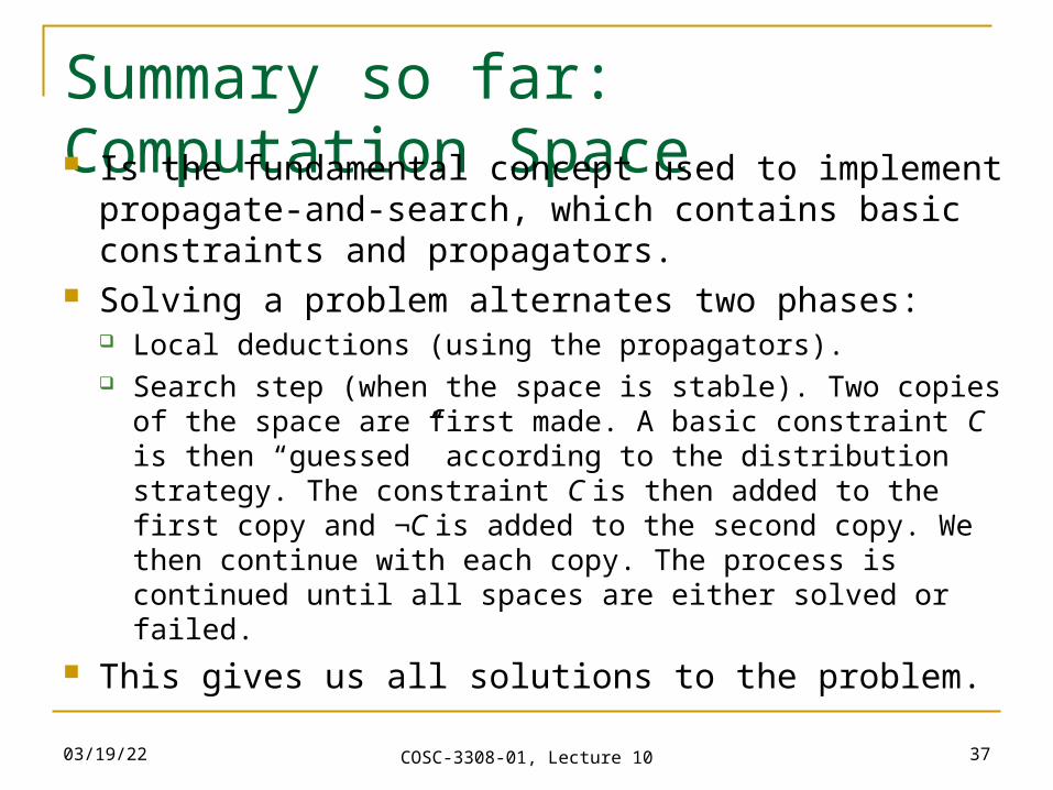
Summary so far: Computation Space Is the fundamental concept used to implement
propagate-and-search, which contains basic constraints and propagators.
Solving a problem alternates two phases: Local deductions (using the propagators). Search step (when the space is stable). Two copies of the
space are first made. A basic constraint C is then “guessed” according to the distribution strategy. The constraint C is then added to the first copy and ¬C is added to the second copy. We then continue with each copy. The process is continued until all spaces are either solved or failed.
This gives us all solutions to the problem.
04/20/23 COSC-3308-01, Lecture 10 38
Constraint Programming in a Nutshell
SEND MORE MONEY
04/20/23 COSC-3308-01, Lecture 10 39
Constraint Programming in a Nutshell
SEND + MORE = MONEY
04/20/23 COSC-3308-01, Lecture 10 40
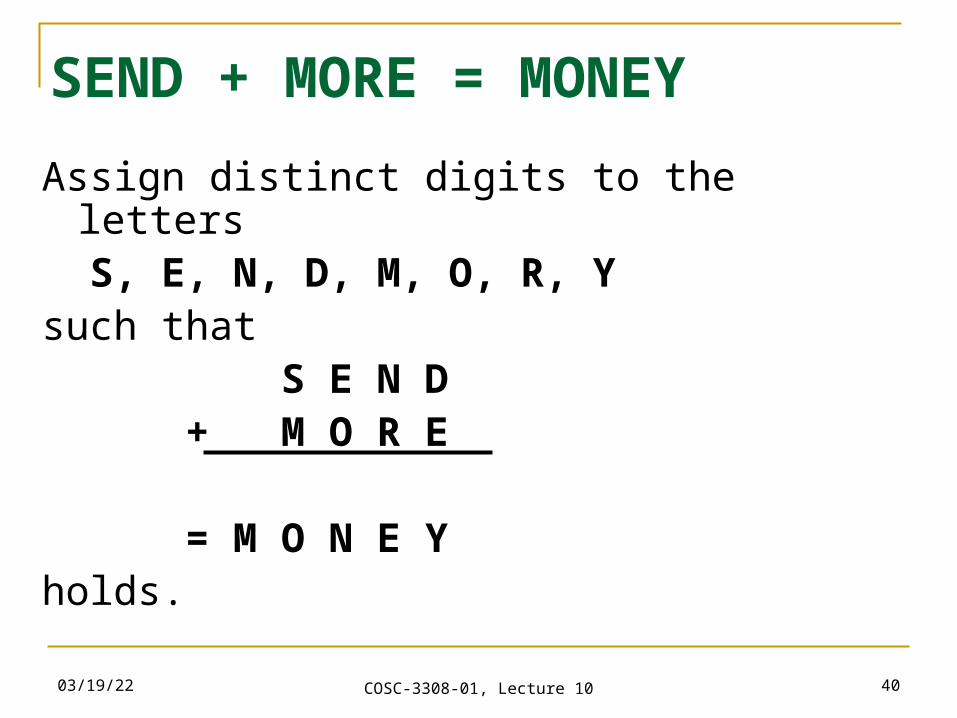
SEND + MORE = MONEY
Assign distinct digits to the letters S, E, N, D, M, O, R, Ysuch that S E N D + M O R E = M O N E Yholds.
04/20/23 COSC-3308-01, Lecture 10 41
SEND + MORE = MONEY
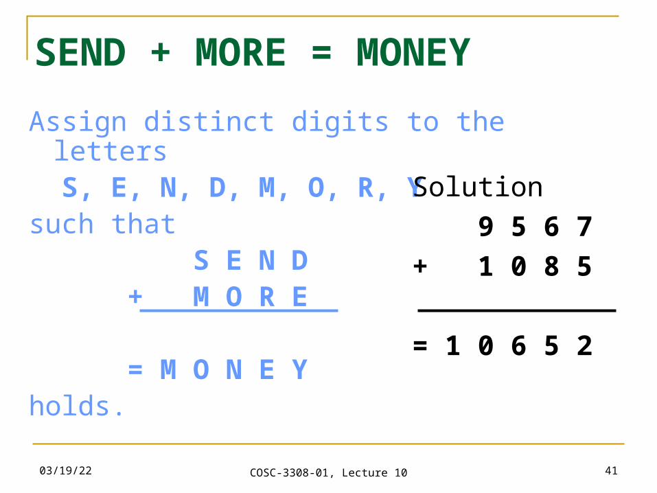
Assign distinct digits to the letters S, E, N, D, M, O, R, Ysuch that S E N D + M O R E = M O N E Yholds.
Solution
9 5 6 7
+ 1 0 8 5
= 1 0 6 5 2
04/20/23 COSC-3308-01, Lecture 10 42
Modeling
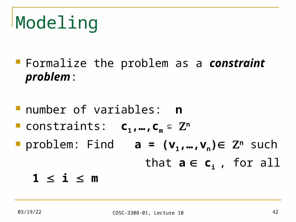
Formalize the problem as a constraint problem:
number of variables: n constraints: c1,…,cm
n
problem: Find a = (v1,…,vn) n such
that a ci , for all 1 i m
04/20/23 COSC-3308-01, Lecture 10 43
A Model for MONEY
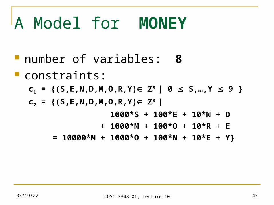
number of variables: 8 constraints: c1 = {(S,E,N,D,M,O,R,Y) 8 | 0 S,…,Y 9 }
c2 = {(S,E,N,D,M,O,R,Y) 8 |
1000*S + 100*E + 10*N + D
+ 1000*M + 100*O + 10*R + E
= 10000*M + 1000*O + 100*N + 10*E + Y}
04/20/23 COSC-3308-01, Lecture 10 44
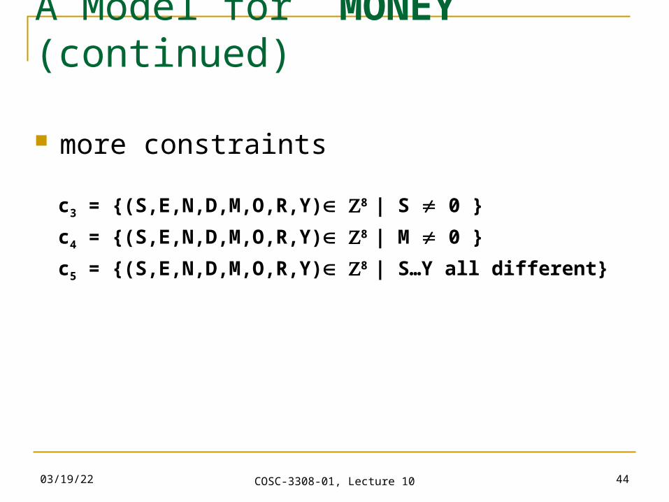
A Model for MONEY (continued)
more constraints
c3 = {(S,E,N,D,M,O,R,Y) 8 | S 0 }
c4 = {(S,E,N,D,M,O,R,Y) 8 | M 0 }
c5 = {(S,E,N,D,M,O,R,Y) 8 | S…Y all different}
04/20/23 COSC-3308-01, Lecture 10 45
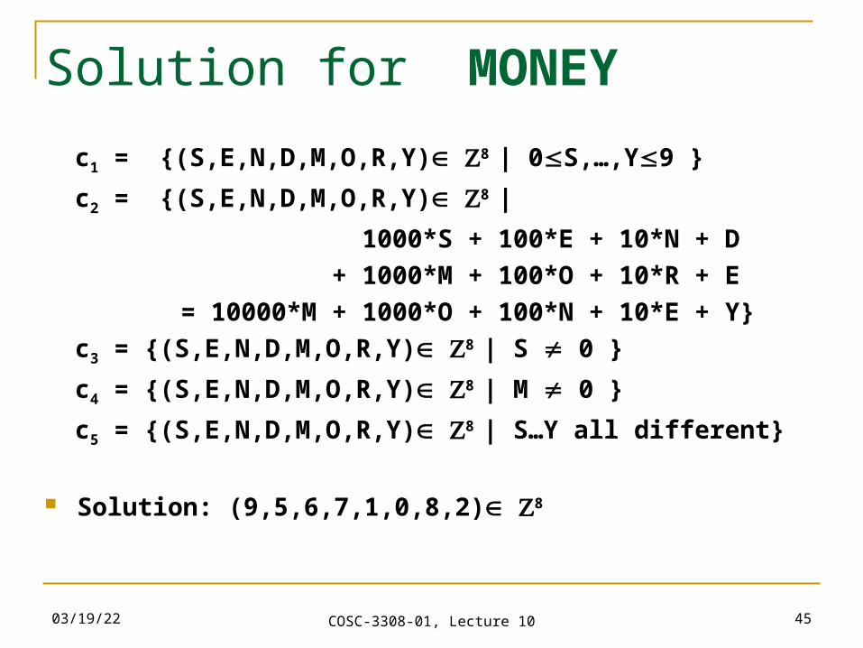
Solution for MONEY
c1 = {(S,E,N,D,M,O,R,Y) 8 | 0S,…,Y9 }
c2 = {(S,E,N,D,M,O,R,Y) 8 |
1000*S + 100*E + 10*N + D
+ 1000*M + 100*O + 10*R + E
= 10000*M + 1000*O + 100*N + 10*E + Y}
c3 = {(S,E,N,D,M,O,R,Y) 8 | S 0 }
c4 = {(S,E,N,D,M,O,R,Y) 8 | M 0 }
c5 = {(S,E,N,D,M,O,R,Y) 8 | S…Y all different}
Solution: (9,5,6,7,1,0,8,2) 8
04/20/23 COSC-3308-01, Lecture 10 46
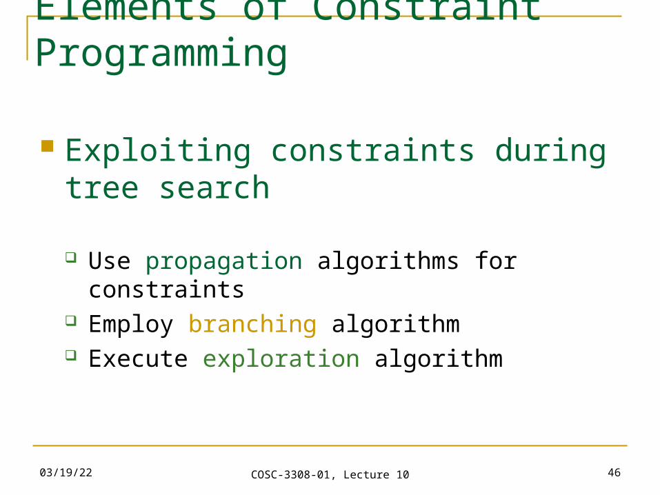
Elements of Constraint Programming
Exploiting constraints during tree search
Use propagation algorithms for constraints Employ branching algorithm Execute exploration algorithm
04/20/23 COSC-3308-01, Lecture 10 47
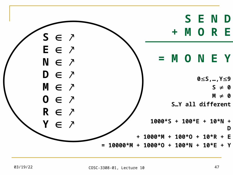
S E N D+ M O R E
= M O N E Y
S E N D M O R Y
0S,…,Y9 S 0M 0
S…Y all different
1000*S + 100*E + 10*N + D
+ 1000*M + 100*O + 10*R + E
= 10000*M + 1000*O + 100*N + 10*E + Y
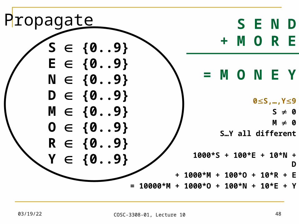
04/20/23 COSC-3308-01, Lecture 10 48
S E N D+ M O R E
= M O N E Y
Propagate
S {0..9}E {0..9}N {0..9}D {0..9}M {0..9}O {0..9}R {0..9}Y {0..9}
0S,…,Y9 S 0M 0
S…Y all different
1000*S + 100*E + 10*N + D
+ 1000*M + 100*O + 10*R + E
= 10000*M + 1000*O + 100*N + 10*E + Y
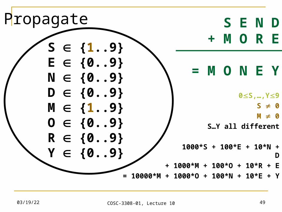
04/20/23 COSC-3308-01, Lecture 10 49
S E N D+ M O R E
= M O N E Y
Propagate
S {1..9}E {0..9}N {0..9}D {0..9}M {1..9}O {0..9}R {0..9}Y {0..9}
0S,…,Y9 S 0M 0
S…Y all different
1000*S + 100*E + 10*N + D
+ 1000*M + 100*O + 10*R + E
= 10000*M + 1000*O + 100*N + 10*E + Y
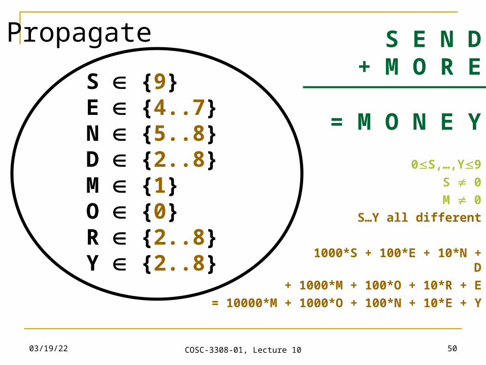
04/20/23 COSC-3308-01, Lecture 10 50
S E N D+ M O R E
= M O N E Y
S {9}E {4..7}N {5..8}D {2..8}M {1}O {0}R {2..8}Y {2..8}
Propagate
0S,…,Y9 S 0M 0
S…Y all different
1000*S + 100*E + 10*N + D
+ 1000*M + 100*O + 10*R + E
= 10000*M + 1000*O + 100*N + 10*E + Y
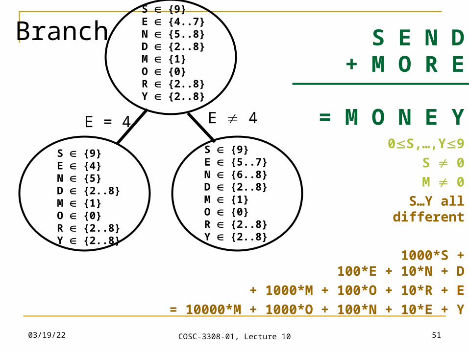
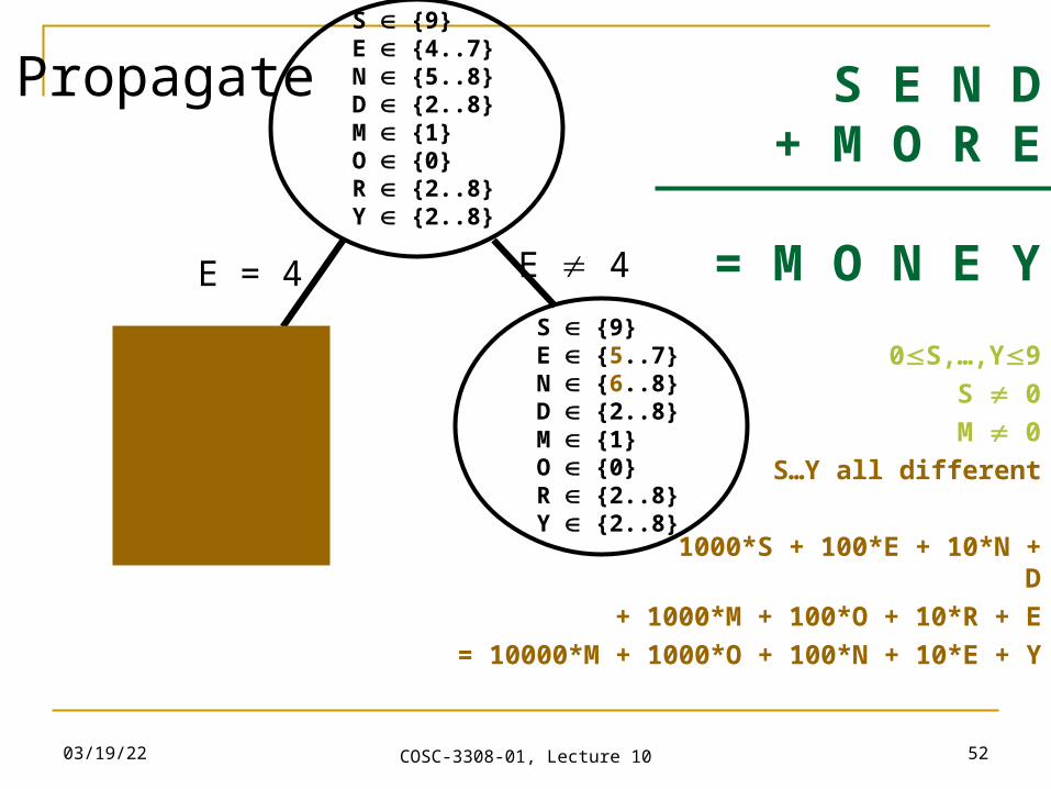
04/20/23 COSC-3308-01, Lecture 10 51
S E N D+ M O R E
= M O N E Y
S {9}E {4..7}N {5..8}D {2..8}M {1}O {0}R {2..8}Y {2..8}
S {9}E {4}N {5}D {2..8}M {1}O {0}R {2..8}Y {2..8}
S {9}E {5..7}N {6..8}D {2..8}M {1}O {0}R {2..8}Y {2..8}
E = 4 E 4
Branch
0S,…,Y9 S 0M 0
S…Y all different
1000*S + 100*E + 10*N + D
+ 1000*M + 100*O + 10*R + E
= 10000*M + 1000*O + 100*N + 10*E + Y
04/20/23 COSC-3308-01, Lecture 10 52
0S,…,Y9 S 0M 0
S…Y all different
1000*S + 100*E + 10*N + D
+ 1000*M + 100*O + 10*R + E
= 10000*M + 1000*O + 100*N + 10*E + Y
S E N D+ M O R E
= M O N E Y
S {9}E {4..7}N {5..8}D {2..8}M {1}O {0}R {2..8}Y {2..8}
S {9}E {5..7}N {6..8}D {2..8}M {1}O {0}R {2..8}Y {2..8}
E = 4 E 4
Propagate
04/20/23 COSC-3308-01, Lecture 10 53
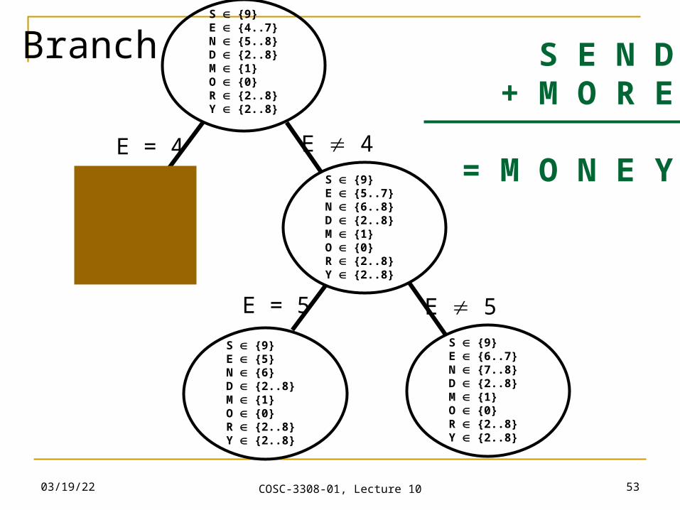
S E N D+ M O R E
= M O N E Y
S {9}E {4..7}N {5..8}D {2..8}M {1}O {0}R {2..8}Y {2..8}
S {9}E {5..7}N {6..8}D {2..8}M {1}O {0}R {2..8}Y {2..8}
E = 4 E 4
Branch
S {9}E {6..7}N {7..8}D {2..8}M {1}O {0}R {2..8}Y {2..8}
E = 5 E 5
S {9}E {5}N {6}D {2..8}M {1}O {0}R {2..8}Y {2..8}
04/20/23 COSC-3308-01, Lecture 10 54
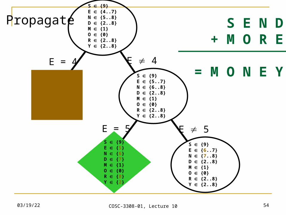
S E N D+ M O R E
= M O N E Y
S {9}E {4..7}N {5..8}D {2..8}M {1}O {0}R {2..8}Y {2..8}
S {9}E {5..7}N {6..8}D {2..8}M {1}O {0}R {2..8}Y {2..8}
E = 4 E 4
Propagate
S {9}E {6..7}N {7..8}D {2..8}M {1}O {0}R {2..8}Y {2..8}
E = 5 E 5S {9}E {5}N {6}D {7}M {1}O {0}R {8}Y {2}
04/20/23 COSC-3308-01, Lecture 10 55
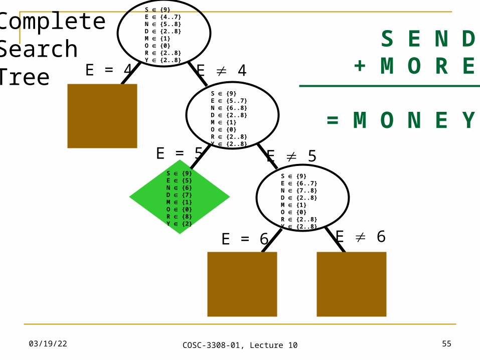
S E N D+ M O R E
= M O N E Y
CompleteSearchTree
S {9}E {4..7}N {5..8}D {2..8}M {1}O {0}R {2..8}Y {2..8}
S {9}E {5..7}N {6..8}D {2..8}M {1}O {0}R {2..8}Y {2..8}
E = 4 E 4
S {9}E {6..7}N {7..8}D {2..8}M {1}O {0}R {2..8}Y {2..8}
E = 5 E 5S {9}E {5}N {6}D {7}M {1}O {0}R {8}Y {2}
E = 6 E 6
04/20/23 COSC-3308-01, Lecture 10 56
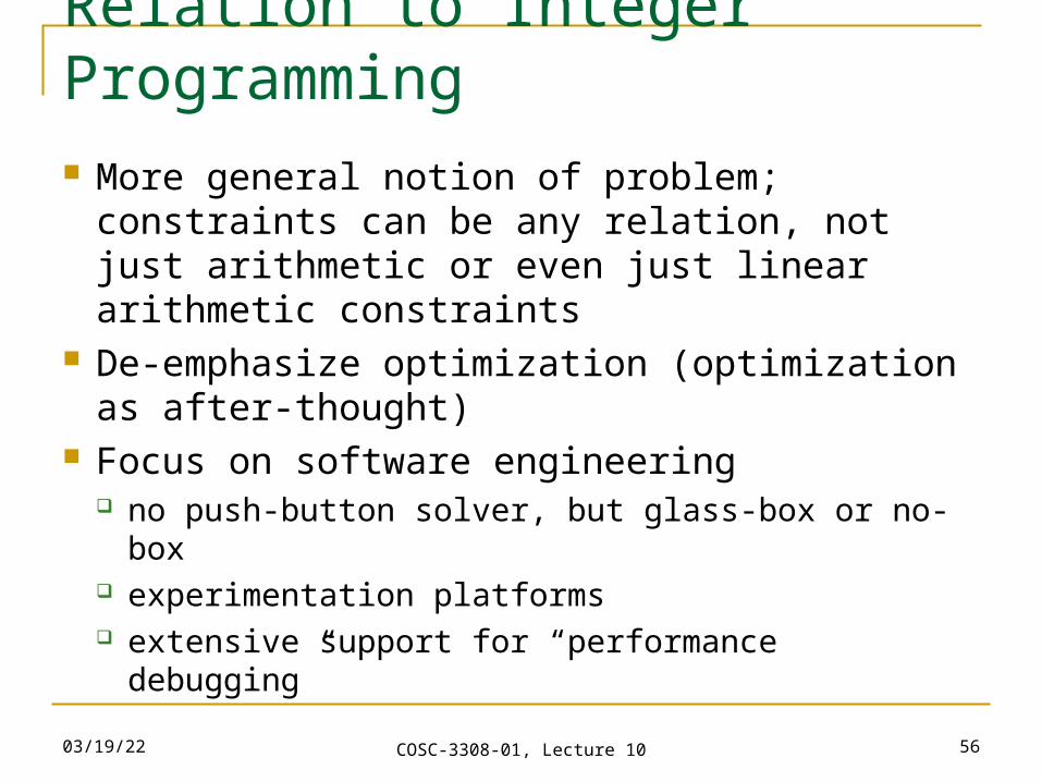
Relation to Integer Programming More general notion of problem; constraints
can be any relation, not just arithmetic or even just linear arithmetic constraints
De-emphasize optimization (optimization as after-thought)
Focus on software engineering no push-button solver, but glass-box or no-box experimentation platforms extensive support for “performance debugging”
04/20/23 COSC-3308-01, Lecture 10 57
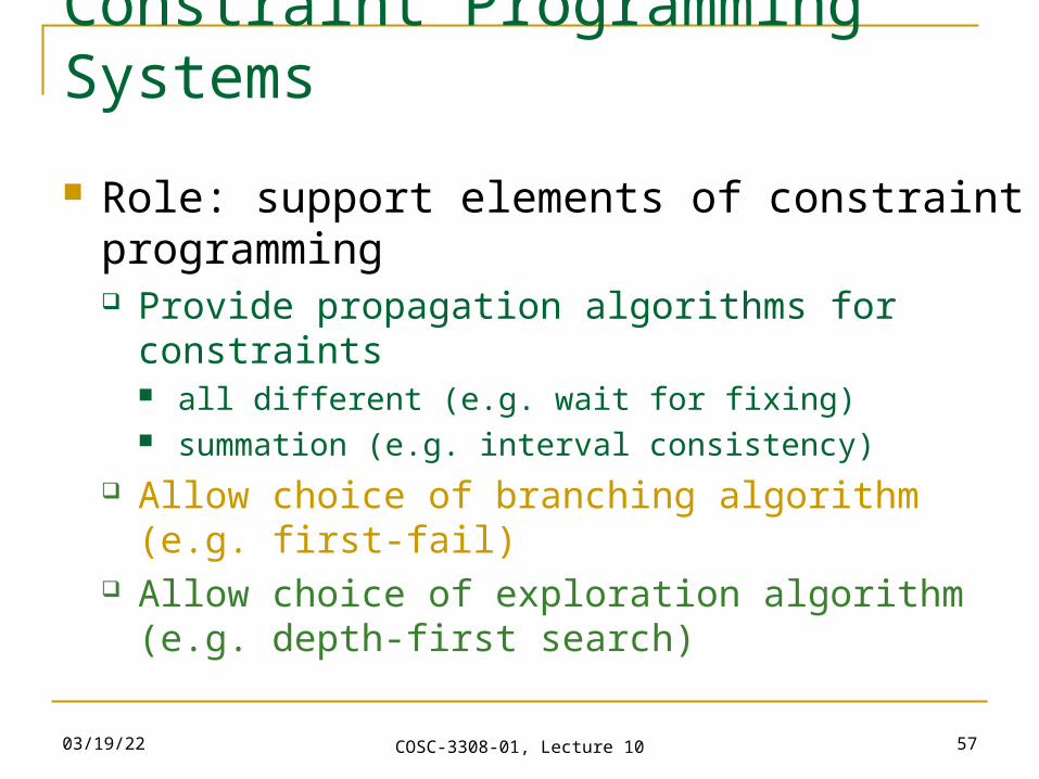
Constraint Programming Systems
Role: support elements of constraint programming Provide propagation algorithms for constraints
all different (e.g. wait for fixing) summation (e.g. interval consistency)
Allow choice of branching algorithm (e.g. first-fail) Allow choice of exploration algorithm (e.g. depth-first
search)
04/20/23 COSC-3308-01, Lecture 10 58
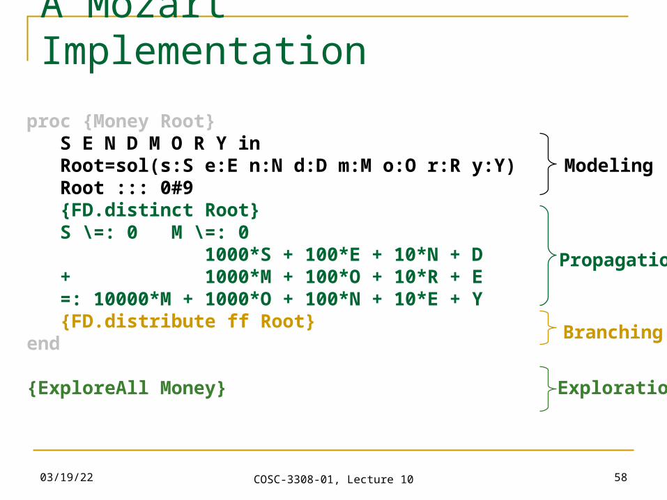
A Mozart Implementation
proc {Money Root} S E N D M O R Y in Root=sol(s:S e:E n:N d:D m:M o:O r:R y:Y) Root ::: 0#9 {FD.distinct Root} S \=: 0 M \=: 0 1000*S + 100*E + 10*N + D + 1000*M + 100*O + 10*R + E =: 10000*M + 1000*O + 100*N + 10*E + Y {FD.distribute ff Root}end
{ExploreAll Money}
Modeling
Propagation
Branching
Exploration
04/20/23 COSC-3308-01, Lecture 10 59
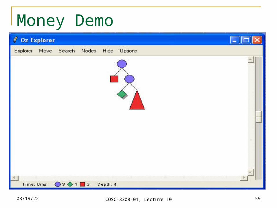
Money Demo
04/20/23 COSC-3308-01, Lecture 10 60
Money Demo
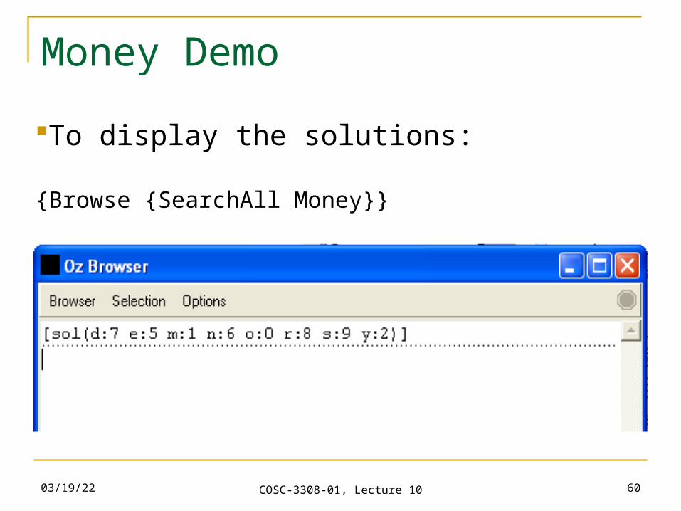
To display the solutions:
{Browse {SearchAll Money}}
04/20/23 COSC-3308-01, Lecture 10 61
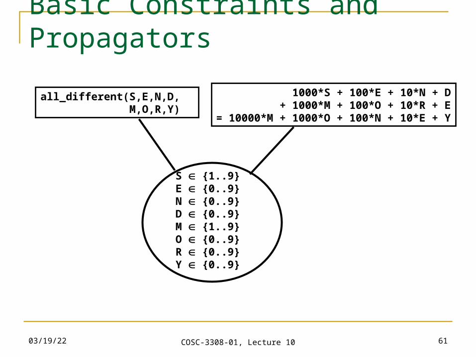
Basic Constraints and Propagators
S {1..9}E {0..9}N {0..9}D {0..9}M {1..9}O {0..9}R {0..9}Y {0..9}
all_different(S,E,N,D, M,O,R,Y)
1000*S + 100*E + 10*N + D + 1000*M + 100*O + 10*R + E= 10000*M + 1000*O + 100*N + 10*E + Y
04/20/23 COSC-3308-01, Lecture 10 62
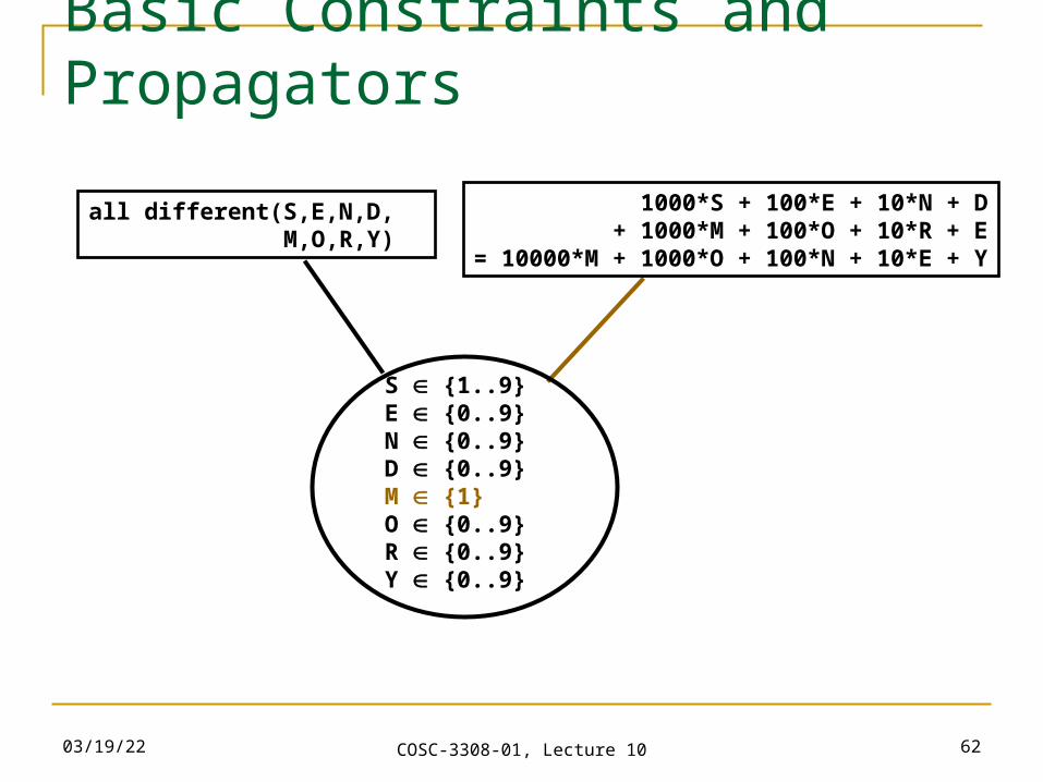
Basic Constraints and Propagators
S {1..9}E {0..9}N {0..9}D {0..9}M {1}O {0..9}R {0..9}Y {0..9}
all different(S,E,N,D, M,O,R,Y)
1000*S + 100*E + 10*N + D + 1000*M + 100*O + 10*R + E= 10000*M + 1000*O + 100*N + 10*E + Y
04/20/23 COSC-3308-01, Lecture 10 63
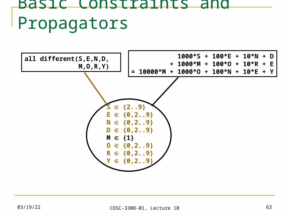
Basic Constraints and Propagators
S {2..9}E {0,2..9}N {0,2..9}D {0,2..9}M {1}O {0,2..9}R {0,2..9}Y {0,2..9}
all different(S,E,N,D, M,O,R,Y)
1000*S + 100*E + 10*N + D + 1000*M + 100*O + 10*R + E= 10000*M + 1000*O + 100*N + 10*E + Y
04/20/23 COSC-3308-01, Lecture 10 64
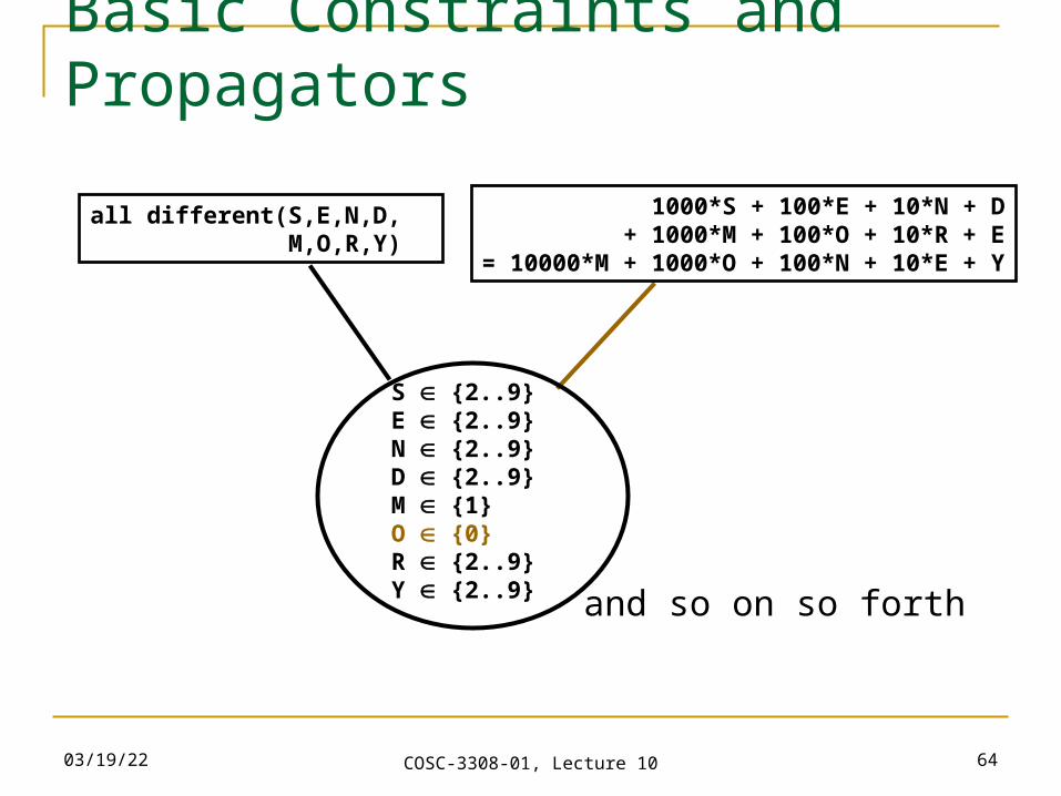
Basic Constraints and Propagators
S {2..9}E {2..9}N {2..9}D {2..9}M {1}O {0}R {2..9}Y {2..9}
all different(S,E,N,D, M,O,R,Y)
1000*S + 100*E + 10*N + D + 1000*M + 100*O + 10*R + E= 10000*M + 1000*O + 100*N + 10*E + Y
and so on so forth
04/20/23 COSC-3308-01, Lecture 10 65
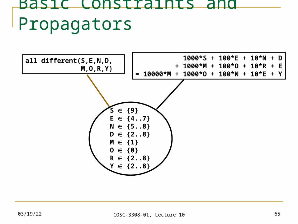
Basic Constraints and Propagators
S {9}E {4..7}N {5..8}D {2..8}M {1}O {0}R {2..8}Y {2..8}
all different(S,E,N,D, M,O,R,Y)
1000*S + 100*E + 10*N + D + 1000*M + 100*O + 10*R + E= 10000*M + 1000*O + 100*N + 10*E + Y
04/20/23 COSC-3308-01, Lecture 10 66
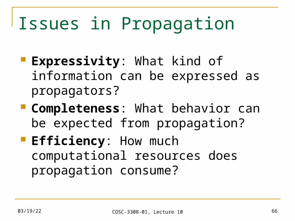
Issues in Propagation
Expressivity: What kind of information can be expressed as propagators?
Completeness: What behavior can be expected from propagation?
Efficiency: How much computational resources does propagation consume?
04/20/23 COSC-3308-01, Lecture 10 67
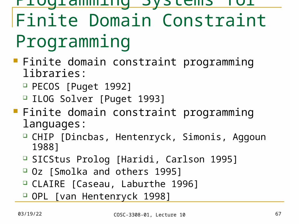
Programming Systems for Finite Domain Constraint Programming Finite domain constraint programming libraries:
PECOS [Puget 1992] ILOG Solver [Puget 1993]
Finite domain constraint programming languages: CHIP [Dincbas, Hentenryck, Simonis, Aggoun 1988] SICStus Prolog [Haridi, Carlson 1995] Oz [Smolka and others 1995] CLAIRE [Caseau, Laburthe 1996] OPL [van Hentenryck 1998]
04/20/23 COSC-3308-01, Lecture 10 68
Summary
Relational programming Choice and Fail Operations
Constraints Programming Basic Constraints, Propagators and Search
04/20/23 COSC-3308-01, Lecture 10 69
Reading suggestions
From [van Roy,Haridi; 2004] Chapter 9, sections 9.1-9.3 Exercises 9.8.1-9.8.5 Chapter 12, sections 12.1-12.3 Exercises 12.4.1-12.4.4
04/20/23 COSC-3308-01, Lecture 10 70
Coming up next
Final-Exam Chapters 1, 2, 3, 4, 5, 6, 7, 9, and 12
04/20/23 COSC-3308-01, Lecture 10 71
Survey of Programming Languages Concepts
COSC-3308-01 is a 3 credit points module Assignments: 30% Mid-Term exam: 20% Tutorials: 10% Written final exam: 40%, open book, December 10,
2010, 8:00 a.m. - 10:30 a.m. (Friday) Lectures: 9:05am-10:00am, room 111, on MWF
Module homepage http://galaxy.cs.lamar.edu/~sandrei/cosc-3308-01
04/20/23 COSC-3308-01, Lecture 10 72
Module Summary Slides: clear + complete (remainder,
summary, definitions, examples, history, motivation, industrial impact, research ideas, comparison with other languages, reading suggestions)
Lab/Assignments 1, 2, 3, 4 Tutorials + Consultation + Email
04/20/23 COSC-3308-01, Lecture 10 73
Motivation for Oz It contains (almost) all the programming language
concepts (declarative, concurrent, stateful, and object-oriented).
We choose such a comprehensive language as Oz for your general knowledge about programming languages.
There exist conferences dedicated to this programming language, such as “International Mozart/Oz Conference” (http://www.cetic.be/moz2004/).
We followed a textbook published at the MIT Press. But … in industry, please don’t expect to have the same
impact factor as Java programming language (for example).
04/20/23 COSC-3308-01, Lecture 10 74
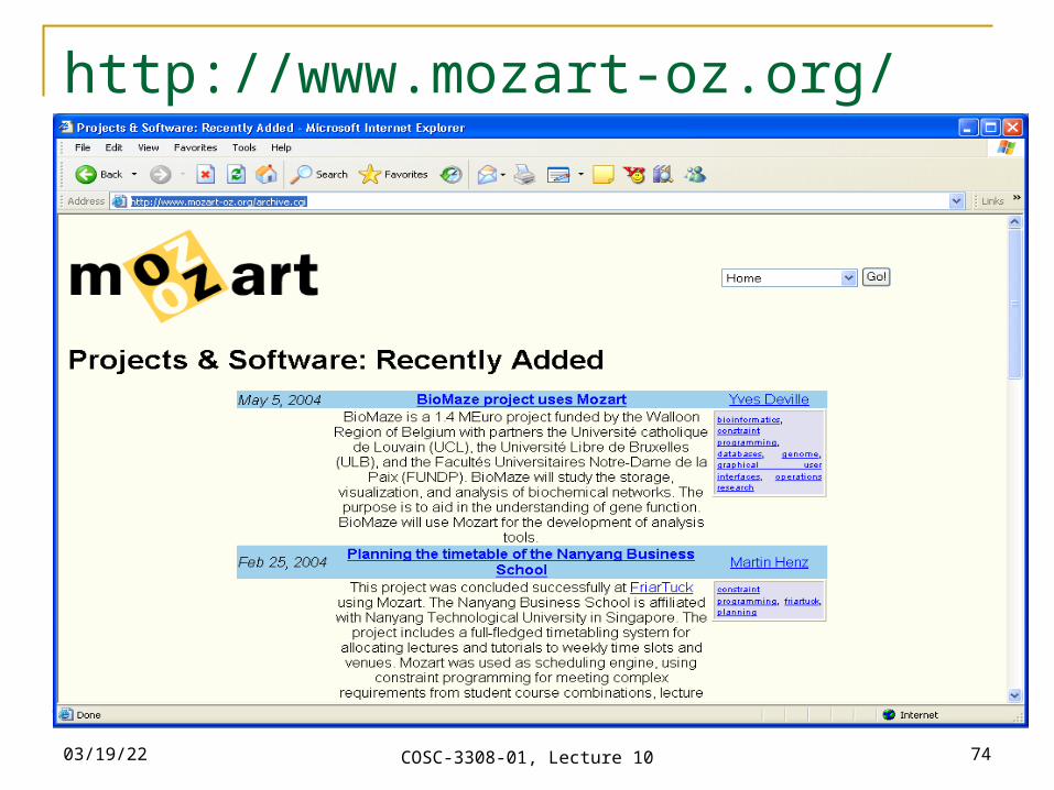
http://www.mozart-oz.org/archive.cgi
04/20/23 COSC-3308-01, Lecture 10 75
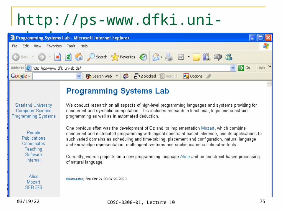
http://ps-www.dfki.uni-sb.de/

04/20/23 COSC-3308-01, Lecture 10 76
Outlook of the Exam Paper
04/20/23 COSC-3308-01, Lecture 10 77
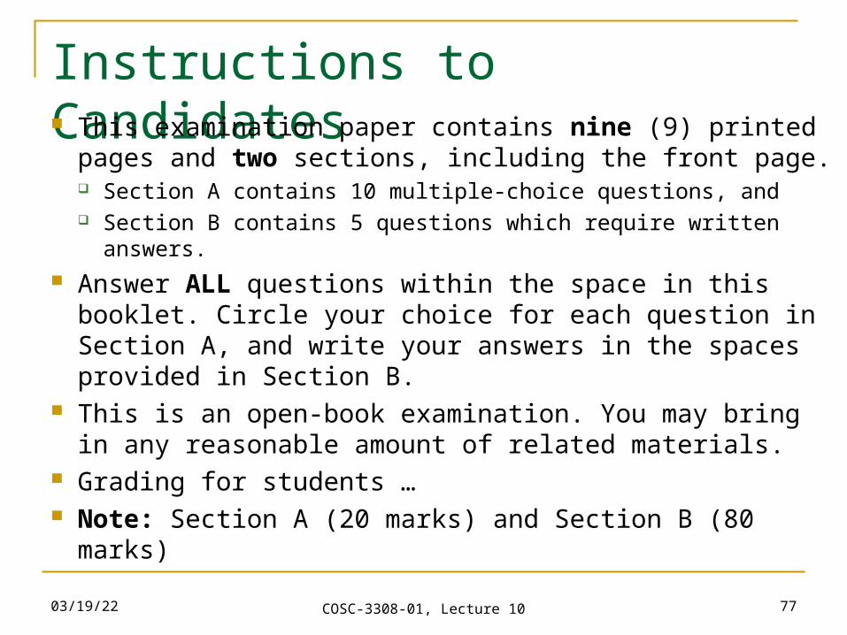
Instructions to Candidates This examination paper contains nine (9) printed pages
and two sections, including the front page. Section A contains 10 multiple-choice questions, and Section B contains 5 questions which require written answers.
Answer ALL questions within the space in this booklet. Circle your choice for each question in Section A, and write your answers in the spaces provided in Section B.
This is an open-book examination. You may bring in any reasonable amount of related materials.
Grading for students … Note: Section A (20 marks) and Section B (80 marks)
04/20/23 COSC-3308-01, Lecture 10 78
Reading and Understanding Suggestions Lectures 1-10 Tutorials 1-10 Lab/Assignments 1-4 Chapters 1, 2, 3, 4, 5, 6, 7, 9, and 12 from
[van Roy,Haridi; 2004]
04/20/23 COSC-3308-01, Lecture 10 79
Thank you for your attention!
Questions?