04/20/23 COSC-4301-01, Lecture 17 1

Real-Time Systems, COSC-4301-01, Lecture 17

Stefan Andrei

04/20/23 COSC-4301-01, Lecture 17 2

Reminder of the last lecture

Modechart – Chapter 6, section 6.8 of [Cheng; 2002]

04/20/23 COSC-4301-01, Lecture 17 3

Overview of This Lecture

Model checking of finite-state systems Chapter 4 of [Cheng; 2002]

04/20/23 COSC-4301-01, Lecture 17 4

Motivation One way to show that a program or system meets the

designer’s specification is to manually construct a proof using axioms and inference rules in a deductive system such as temporal logic, a first-order logic capable of expressing relative ordering of events.

This traditional (and manual approach) to concurrent program verification is tedious and error-prone even for small programs.

For finite-state (concurrent) systems, we can use model checking instead of proof construction to check their correctness relative to their specification.

04/20/23 COSC-4301-01, Lecture 17 5

Model checking approach Represents the (concurrent) system as a finite-state

graph, which can be viewed as a finite Kripke structure. The specification and/or safety assertion is/are

expressed in propositional temporal logic formulas. We can then check whether the system meets its

specification using an algorithm called a model checker. So, the model checker determines whether the Kripke

structure is a model of the formula(s). Example of model checkers:

[Clarke, Emerson, Sistla; 1986] [Burch, et al; 1990]

04/20/23 COSC-4301-01, Lecture 17 6

[Clarke, Emerson, Sistla; 1986]’s approach The system to be checked is represented by a labeled

finite-state graph and the specification is written in a propositional, branching-time temporal logic called computation tree logic (CTL).

The use of linear-time temporal logic (LTL), which can express fairness properties, is ruled out since a model checker such as a logic has high complexity.

Instead, fairness requirements are moved into the semantics of CTL.

We use the terms program and system interchangeably.

04/20/23 COSC-4301-01, Lecture 17 7

System specification To construct the finite-state graph corresponding to a

given concurrent program, we can begin with the initial state labeled with the initial values of all program variables or attributes (called labels here).

For each possible statement, we execute the statement and examine any change to one or more program variables.

We construct a new state if it is different from any existing state, together with an edge between these states.

We repeat this state and edge construction steps until there are no states to consider.

04/20/23 COSC-4301-01, Lecture 17 8

Finite-state graph. Railroad crossing CTL structure for the railroad crossing system:

Figure 4.1 of [Cheng; 2005], page 88

04/20/23 COSC-4301-01, Lecture 17 9

The CTL structure The CTL structure (state graph) is a triple,

M=(S, R, P), where: S is a finite set of states, R is a binary relation on S which gives the possible

transitions between states, P assigns to each state the set of atomic

propositions true in that state. Example:

The previous figure shows each state with two variables (gate-position, train-position).

The initial state is S0.

04/20/23 COSC-4301-01, Lecture 17 10

The correctness of hardware and software systems

Four principal techniques for ensuring the correctness of hardware and software systems: Simulation Testing Deductive Verification Model Checking

04/20/23 COSC-4301-01, Lecture 17 11

System Verification System Verification via Model Checking What is Model Checking? Comparison with other techniques

04/20/23 COSC-4301-01, Lecture 17 12

The Process of Model Checking Three Steps of the Model Checking

modeling specification verification.

04/20/23 COSC-4301-01, Lecture 17 13

Step 1 --- Modeling Modeling is the conversion of the system into

a formalism. For modeling of systems we use finite

automata. Owing to limitations on time and memory, the

modeling of a design may require the use of abstraction.

We use a type of state transition graph called a Kripke structure to model a system.

04/20/23 COSC-4301-01, Lecture 17 14

The Kripke structure A Kripke structure over a set of atomic

propositions AP is a four-tuple, M = (S, S0, R, L), where S is a finite set of states. S0 S is the set of initial states. R S × S is a transition relation. L: S2AP is a function that labels each state

with the set of atomic propositions true in this state.

04/20/23 COSC-4301-01, Lecture 17 15

Kripke-Structure. Micro-oven cooking Example

04/20/23 COSC-4301-01, Lecture 17 16

Kripke-Structure. Micro-oven cooking Example M = (S, S1, R, L)

S = {S1, S2, S3, S4} S1 is the initial state. R = {(S1, S2), (S2, S1), (S1, S4), (S4, S2), (S2, S3),

(S3, S2), (S3, S3)} L (S1) = {¬close, ¬start, ¬cooking} L (S2) = {close, ¬start, ¬cooking} L (S3) = {close, start, cooking} L (S4) = {¬close, start, ¬cooking}

04/20/23 COSC-4301-01, Lecture 17 17

Step 2 --- Specification

What is Specification? Classical Logic Temporal Logic

04/20/23 COSC-4301-01, Lecture 17 18

Operators for the Temporal Logic Four basic temporal operators:

1. X (‘‘next time’’)

2. F (‘‘in the future’’)

3. G (‘‘globally’’)

4. U (‘‘until’’) Two quantifiers for the Temporal Logic:

1. A (‘‘always’’)

2. E (‘‘exists’’)

04/20/23 COSC-4301-01, Lecture 17 19

Three main ways to represent Temporal Logic:

CTL* (Computation Tree Logic*). CTL (Computation Tree Logic) with 8 basis

operators: AX and EX; AF and EF; AG and EG;

AU and EU. LTL (Linear Temporal Logic).

04/20/23 COSC-4301-01, Lecture 17 20

Semantics of CTL operators Literal p holds in state s iff p L(s). Formula ¬ holds in s iff does not hold in s. Formula 1 2 holds in s iff 1 and 2 hold in s.

Formula 1 2 holds in s iff 1 or 2 holds in s.

Formula 1 2 holds in s iff 1 does not hold in s or 2 hold in s.

Formula AX holds in s iff holds for all direct successors of s.

Formula EX holds in s iff holds for some direct successors of s.

04/20/23 COSC-4301-01, Lecture 17 21

Semantics of CTL operators Formula AG holds in s iff holds for all paths

beginning in s. A path is a set of states that are linked by arcs in the Kripke

structure. Formula holds for a path iff it holds for all states of that

path. Formula EG holds in s iff holds for a path

beginning in s. Formula AF holds in s iff for all paths beginning in s

then holds for some successor of s. Formula EF holds in s iff there is a path beginning in

s such that holds for some successor of s.

04/20/23 COSC-4301-01, Lecture 17 22

Semantics of CTL operators

Formula 1 U 2 holds in s iff there is a path beginning in s (say s=s1 s2 …) for which there exists si such that 2 holds in si and 1 holds in s1, …, si-1.

Formula A[1 U 2] holds in s iff all paths beginning in s satisfy 1 U 2.

Formula E[1 U 2] holds in s iff there is a path beginning in s that satisfies 1 U 2.

04/20/23 COSC-4301-01, Lecture 17 23

Model checking

Goal: Determine whether a formula holds in a state.

Problem: Formulas refer to infinite paths.

Solution: Only interested in checking sub-formulas at states. Collect states where sub-formulas are true.

Key observation: The number of states is finite.

04/20/23 COSC-4301-01, Lecture 17 24

Step 3 --- Verification

CTL* - Model-Checking CTL - Model-Checking LTL - Model-Checking Human assistance ? + Error trace

04/20/23 COSC-4301-01, Lecture 17 25

Verification

04/20/23 COSC-4301-01, Lecture 17 26

Algorithms for Model Checking State space explosion problem Number of states typically grows

exponentially in the number of process

04/20/23 COSC-4301-01, Lecture 17 27

Exponentially growing

04/20/23 COSC-4301-01, Lecture 17 28

The major techniques for tackling this problem

Based on Automata Theory Based on Symbolic Structure Other Methods -- Alternative Methods

04/20/23 COSC-4301-01, Lecture 17 29

Based on Automata Theory (1) On the Fly Technology

Definition Intersection in the “on-the-fly” model checking Advantage of on-the-fly model checking

04/20/23 COSC-4301-01, Lecture 17 30

Based on Automata Theory (2) Partial-Order Reduction Technologies

1. what is interleaving?

2. what is partial-order representation?

3. three kinds of the partial-order reduction technologies

dynamic partial-order reduction technology static partial-order reduction technology purely partial-order reduction technology

04/20/23 COSC-4301-01, Lecture 17 31

Based on Symbolic Structure

Symbolic Structure with a Boolean formula Binary Decision Diagram (BDD) 105 states -- 1020 states -- 10120 states SMV language and OBDD (Bryant's ordered

binary decision diagrams) Successful examples with SMV

04/20/23 COSC-4301-01, Lecture 17 32

Example When concurrent processes share a resource, it may

be necessary to ensure that they do not have access to it at the same time.

The solution should satisfy: Safety: the protocol allows only one process to be in its

critical section at any time. Liveness: whenever any process wants to enter its critical

section, it will eventually be permitted to do so. Non-blocking: a process can always request to enter its

critical section. No strict sequencing: processes need to enter their critical

section in strict order.

04/20/23 COSC-4301-01, Lecture 17 33

Modeling two processes

Each process can be in: Non-critical state (N) Trying to enter in its critical state (T) In its critical state/section (C)

Each individual process undergoes transitions in the cycle N T C N …, but the two processes interleave with each other.

04/20/23 COSC-4301-01, Lecture 17 34

First attempt of mutual exclusion

N1,N2

T1,N2

C1,T2

N1,T2

C1,N2

T1,T2

N1,C2

T1,C2

s0

s1

s3

s5

s2

s7

s4

s6

04/20/23 COSC-4301-01, Lecture 17 35

Verification of the four properties Safety: 1 = AG ¬(C1 C2).

Liveness: 2 = AG (T1 AF C1) and of course one similar for the second process: AG (T2 AF C2).

Non-blocking: 3 = AG (N1 EX T1) and of course AG (N2 EX T2).

No strict sequencing: 4 = EF (C1 E[C1 U (¬C1 E[¬C2 U C1])]) and

of course one similar for the second process: EF (C2 E[C2 U (¬C2 E[¬C1 U C2])])

04/20/23 COSC-4301-01, Lecture 17 36

Verifying Safety

1 = AG ¬(C1 C2) Clearly, ¬(C1 C2) is satisfied in the initial

state. So it is satisfied in every state because no

state has both C1 and C2.

04/20/23 COSC-4301-01, Lecture 17 37

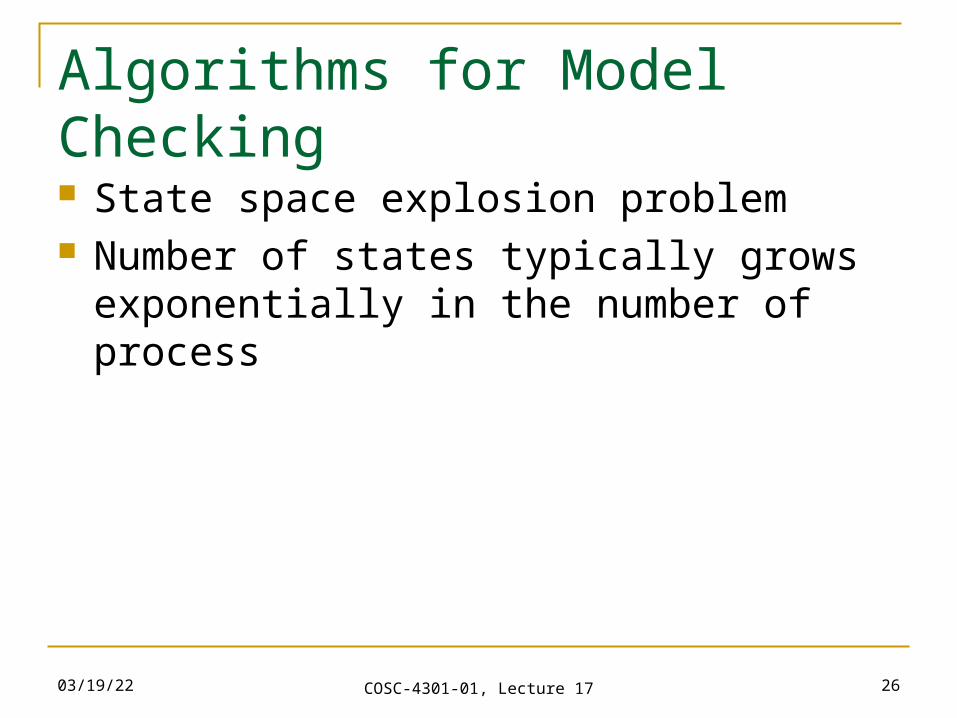
Verifying Liveness

2 = AG (T1 AF C1) This is not satisfied by the initial state. We can find a state accessible from the initial

state, namely s1, in which T1 is true, but AF C1 is false, because there is a computation path s1 s3 s7 s1 … on which C1 is always false!

So 2 does not hold.

04/20/23 COSC-4301-01, Lecture 17 38

Verifying Non-blocking

3 = AG (N1 EX T1)

Every N1 state (s0, s5 and s6) has an immediate T1 successor.

So 3 holds.

04/20/23 COSC-4301-01, Lecture 17 39

Verifying No strict sequencing 4 = EF (C1 E[C1 U (¬C1 E[¬C2 U C1])]) This is satisfied by the mirror path to the

computation path described for liveness, s5 s3 s4 s5 …

So 4 holds.

04/20/23 COSC-4301-01, Lecture 17 40

The second attempt

The reason liveness failed in our first attempt at modeling mutual exclusion is that non-determinism means it might continually favour one process over another.

The problem is that s3 does not distinguish between which of the processes first went to its trying state.

To fix this, we split s3 into two states.

04/20/23 COSC-4301-01, Lecture 17 41

Second attempt of mutual exclusion

N1,N2

T1,N2

C1,T2

N1,T2

C1,N2 T1,T2 T1,T2 N1,C2

T1,C2

s0

s1

s2s3

s4

s5

s8 s6

s7

04/20/23 COSC-4301-01, Lecture 17 42

Exercise

Verify the four properties for this new model.

04/20/23 COSC-4301-01, Lecture 17 43

The labeling algorithm Given a model M and a CTL formula , the

labeling algorithm outputs the set of states of the model that satisfy .

The CTL formula has only the connectives: , , , AF, EU, and EX (the others can be expressed using these connectives).

Next, we label the states of M with the sub-formulas of that are satisfied there, starting with the smallest sub-formulas and working towards .

04/20/23 COSC-4301-01, Lecture 17 44

Steps of the labeling algorithm Suppose is a sub-formula of and states

satisfying all the immediate sub-formulas of have already been labeled.

If is : then no states are labeled with . p: then label s with p if p L(s). 1 2: label s with 1 2 if s is already labeled with

both 1 and with 2. 1: label s with 1 if s is not already labeled with 1. EX 1: label any state with EX 1 if one of its

successors is labeled with 1.

04/20/23 COSC-4301-01, Lecture 17 45

Steps of the labeling algorithm (cont) AF 1:

If any state s is labeled with 1, label it with AF 1.

Repeat: label any state with AF 1 if all successors states are labeled with AF 1, until there is no change.

Figure 3.24 from [Huth and Ryan; 2004], page 223

04/20/23 COSC-4301-01, Lecture 17 46

Steps of the labeling algorithm (cont) E [1 U 2]

If any state s is labeled with 2, label it with E [1 U 2].

Repeat: label any state with E [1 U 2] if it is labeled with 1 and at least one of its successors is labeled with E [1 U 2], until there is no change.

Figure 3.25 from [Huth and Ryan; 2004], page 224

04/20/23 COSC-4301-01, Lecture 17 47

Example Checking E [c2 U c1] for mutual exclusion model. The labeling algorithm labels all states that have c1

during phase 1 with E [c2 U c1]: states s2 and s4.

During phase 2, it labels all states that does not satisfy c2 and have a successor state that is already labeled: states s1 and s3.

During phase 3, we label s0 because it does not satisfy c2 and has a successor state (s1) which is already labeled.

Thereafter, the algorithm terminates because no additional states get labeled: all unlabelled states either satisfy c2, or must pass through such a state to reach a labeled state.

04/20/23 COSC-4301-01, Lecture 17 48

Example (cont)Figure 3.27 from [Huth and Ryan; 2004], page 226

04/20/23 COSC-4301-01, Lecture 17 49

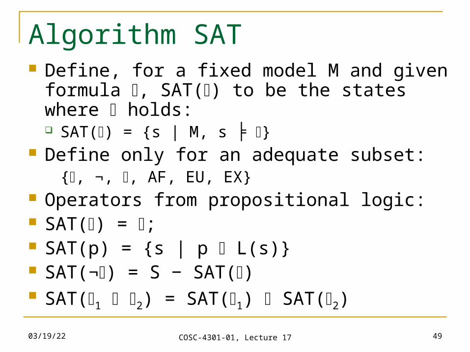
Algorithm SAT Define, for a fixed model M and given formula

, SAT() to be the states where holds: SAT() = {s | M, s ╞ }

Define only for an adequate subset:{, ¬, , AF, EU, EX}

Operators from propositional logic: SAT() = ; SAT(p) = {s | p L(s)} SAT(¬) = S − SAT() SAT(1 2) = SAT(1) SAT(2)

04/20/23 COSC-4301-01, Lecture 17 50

Algorithm SAT. Example

04/20/23 COSC-4301-01, Lecture 17 51

Algorithm SAT (cont)

SAT(1 2) = SAT(1) SAT(2)

SAT(1 2) = SAT(¬1 2) SAT(AX ) = SAT(¬EX ¬) SAT(EX ) = {s | s’.s s’ s’ SAT()} More algorithmically:

X = SAT(); Y = {s | s’.s s’ s’ X}; return Y;

04/20/23 COSC-4301-01, Lecture 17 52

Algorithm SAT (cont)

SAT(A[1 U 2]= SAT(¬E(¬2 U (¬1 ¬2)] EG ¬2)

SAT(E[1 U 2]) is given algorithmically by: W := SAT(1); X := ; Y := SAT(2); while (X ≠ Y) {

X := Y; Y := Y (W {s | s’.s s’ and s’ Y });

} return Y;

04/20/23 COSC-4301-01, Lecture 17 53

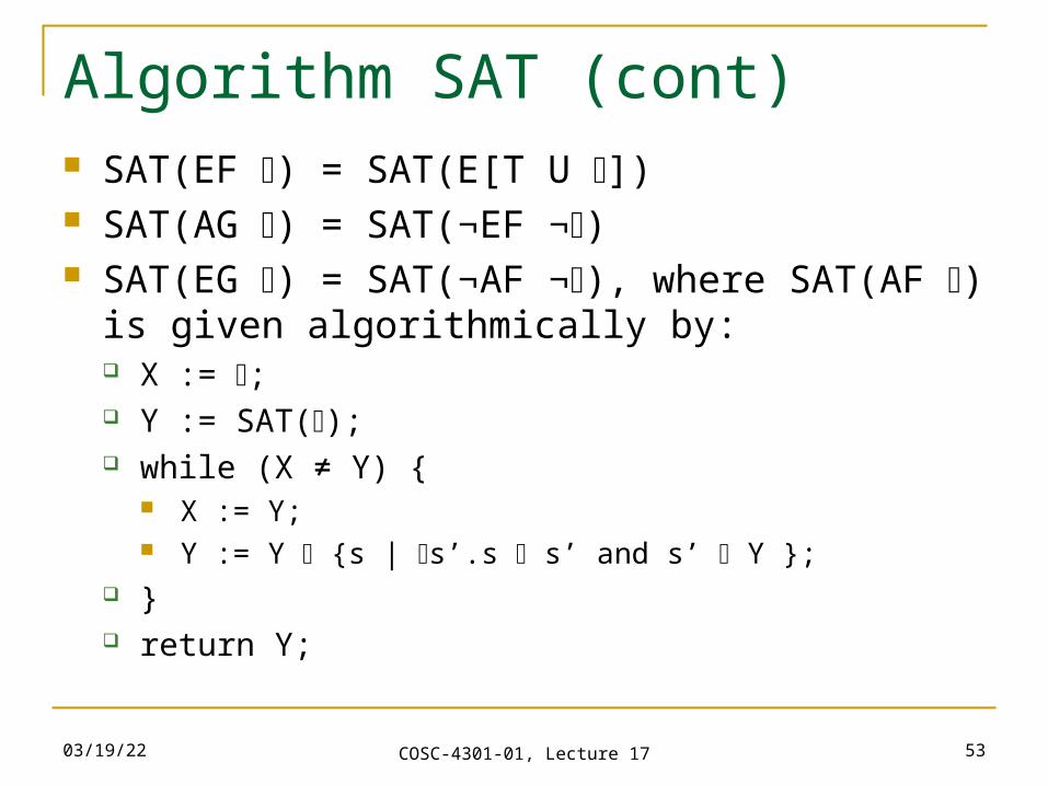
Algorithm SAT (cont) SAT(EF ) = SAT(E[T U ]) SAT(AG ) = SAT(¬EF ¬) SAT(EG ) = SAT(¬AF ¬), where SAT(AF ) is

given algorithmically by: X := ; Y := SAT(); while (X ≠ Y) {

X := Y; Y := Y {s | s’.s s’ and s’ Y };

} return Y;

04/20/23 COSC-4301-01, Lecture 17 54

Microwave-oven cooking. Example Specification with CTL-Formal:

AG (start AF cooking) AG ((close start) AF cooking)

04/20/23 COSC-4301-01, Lecture 17 55

Microwave-oven cooking. Example 1 CTL-Formula: AG (start AF cooking)

1. Change formal to ¬EF (start EG ¬cooking))2. From simple partial formulas to the more complicated

formulas, until all of the formulas are true. S (start) = {S3, S4} S (¬cooking) = {S1, S2, S4} S (EG ¬cooking) = {S1, S2, S4} (all conditions lie on a path) S (start EG ¬cooking) = {S4} S (EF (start EG ¬cooking)) = {S1, S2, S3, S4} (can be followed

with S4) S (¬(EF (start EG ¬cooking))) = { }

3. Result analyze: the initial formula is not a theorem (it does not hold in any of the states of Kripke structure)

04/20/23 COSC-4301-01, Lecture 17 56

Microwave-oven cooking. Example 2 CTL-Formula: AG ((close start) AF cooking)

1. Change formal to ¬EF(close start EG ¬cooking)2. Now the algorithm can be applied to the formula

S (close)= {S2, S3} S (start)= {S3, S4} S (¬cooking) = {S1, S2, S4} S (EG ¬cooking) = {S1, S2, S4} S (close start EG ¬cooking) = { } S (EF (close start EG ¬cooking) = { } S (¬(EF (close start EG ¬cooking)) = {S1, S2, S3, S4}

3. Result analyze: the initial formula is a theorem (it holds in all the states of Kripke structure)

04/20/23 COSC-4301-01, Lecture 17 57

Real-Time CTL

Existentially Bounded Until operator:

E[f1 U[x,y] f2] at state s0 means there exists a path beginning at s0 and some i such that x <= i <= y and f2 holds at state si and for all j < i, f1 holds at state sj

Min/max delays Min/max number of condition occurrences

04/20/23 COSC-4301-01, Lecture 17 58

Summary

Model checking of finite-state systems

04/20/23 COSC-4301-01, Lecture 17 59

Reading suggestions

Chapter 4 of [Cheng; 2005] Chapter 4 of [Huth and Ryan; 2004], where

this is: M. Huth and M. Ryan: Logic in Computer Science.

Modelling and Reasoning about Systems. Cambridge University Press, 2004, ISBN 978-0521-543101

04/20/23 COSC-4301-01, Lecture 17 60

Coming up next

Symbolic model checking of finite-state systems

(Ordered) Binary Decision Diagrams Chapter 4 of [Cheng; 2002]

04/20/23 COSC-4301-01, Lecture 17 61

Thank you for your attention!

Questions?