Embed Size (px)
Citation preview
INVESTIGATION OF QUEUEING PARAMETERS
FOR
EVALUATING
BOSTON HOUSING AUTHORITY MAINTNENANCE OPERATIONS
by
Theodore James Langton
B.A. Hampshire CollegeAmherst, Massachusetts
(1980)
Submitted to the Department ofUrban Studies and Planning
in Partial Fulfillment of theRequirements of the
Degree of
MASTER OF CITY PLANNING
at the
MASSACHUSETTS INSTITUTE OF TECHNOLOGY
June 1984
c Theodore J. Langton 1984
The author hereby grants to M.I.T. permission to reproduce and to distributecopies of this thesis document in whole or in part.
Signature of Author . -- --
Department of Urban Studies and Pl nning, 23 May 1984
Certified byAaron Fleisher
Thesis Supervisor
Accepted by
HUSETTS gisTOTECHN~Lwy
Ralph Gakenheimer, ChairmanDepartmental Graduate Committee
AUG 101984LIRAPiE3 otch
MA
i

ii
"Investigation of Queueing Parametersfor
EvaluatingBoston Housing Authority Maintenance Operations"
Masters Thesis in City PlanningTheodore Langton
Masachusetts Institute of TechnologyJune 1984
ABSTRACT
This paper analyses current problems in evaluating BHAmaintenance operations using recorded data, offers suggestions fordesigning monthly performance measures, and discusses criteria forevaluating proposed operations policies. On the assumption thataccurate projections of demand are preferable to strict preschedulingas a basis for designing maintenance systems that are responsive totenants needs, I have investigated the conditions necessary for usingstochastic queueing models to project the consequences of alternativeoperating policies.
The analysis uses Consistent System statistical programsdeveloped by the Laboratory of Architecture & Planning at MIT and runon the Multics operating system at MIT's Information ProcessingServices. In Chapter I the relationship of data structure tomaintenance operations is described and variables are chosen fromOctober 1983 work order data provided by the BHA. I then usetechniques from linear regression, analysis of variance, goodness offit tests and queueing theory in Chapter III to define the behavior ofwork order arrival processes. A similar analysis is presented forservice times in Chapter IV.
The results suggest that calls for service are not Poissondistributed, although the limited sample size makes it difficult todraw definitive conclusions. I also test the sensitivity of variousmethods for comparing observed and hypothesized probabilitydistributions at different arrival rates and sample sizes. Because itis likely that systematic maintenance problems are causing work ordersto be generated non-randomly, a method is outlined for identifyingbuilding systems failures from task code data to be recorded by amodified work order processing system. The extent to which work ordersare generated in a Poisson manner can then be used as one measure ofhow well buildings are being maintained.
Chapter IV provides reasonable evidence that service times arenot exponentially distributed and suggests that queue interdependencymay explain observed service time distributions. Poisson-basedqueueing models therefore would not currently provide acceptableaccuracy for use in evaluating proposed operating policies.
I then use more generally applicable relationships from queueingtheory in Chapter V to analyze turn-around times and queue lengths,and to compare priority policies. First, a regression model indicatesthat service priority is given to recent work orders rather than toemergencies per se. The tendency to delay the service of older workorders creates backlogs which are not fully reflected in mean
ii
turn-around times. In addition, since several work orders may begenerated for a single repair job, it is difficult to estimate thenumber of tenants in queue. The resulting ambiguities are notprimarily due to data structure, however, but to operating problems.Although the number of servers appears adequate, inefficientpriority-of-service policies and interdependent queues seriouslyhinder the system's responsiveness to demand. Therefore, suggestionsare made for reducing interdependency and a method is described forcomparing priority policies with respect to total expected waitingtimes.

i i i
Acknowledgements
I would like to warmly thank Aaron Fleisher, Professor of UrbanStudies & Planning, and Statistics Instructor Ed Kaplan at MIT fortheir time, teaching, suggestions, criticisms, encouragement andinspiration. I am also grateful to Gwen Friend, Ricardo Duran and theBoston Housing Authority for the time and effort they generouslydonated, and for the use of their information. Then there are myparents, whom I can never thank enough, and Cynthia Lagier - who didthe graphics, who understands what the Poisson distribution is allabout, and to whom I was a phantom for several months.

iv
"The first intimation that things were getting out of hand came
one early-fall evening in the late nineteen forties. What happened,
simply, was that between seven and nine o'clock on that evening the
Triborough Bridge had the heaviest concentration of outbound traffic
in its entire history...The bridge personnel, at any rate, was caught entirely unprepared.
A main artery of traffic, like the Triborough, operates under fairly
predictable conditions. Motor travel, like most other large-scale
human activities, obeys the Law of Averages - that great, ancient rule
that states that the actions of people in the mass will always follow
consistent patterns - and on the basis of past experience it had
always been possible to foretell, almost to the last digit, the number
of cars that would cross the bridge at any given hour of the day or
night. In this case, though, all rules were broken...
The incident was unusual enough to make all the front pages next
morning, and because of this many similar events, which might
otherwise have gone unnoticed, received attention... It was apparent
at last that something decidedly strange was happening. Lunchroom
owners noted that increasingly their patrons were developing a habit
of making runs on specific items; one day it would be the roast
shoulder of veal with pan gravy that was ordered almost exclusively,
while the next everyone would be taking the Vienna loaf and the roast
veal went begging. A man who ran a small notions store in Bayside
revealed that over a period of 4 days, 274 successive customers had
entered his shop and asked for a spool of pink thread...
At this juncture it was inevitable that Congress should be called
on for action... In the course of the committee's investigations it
had been discovered, to everyone's dismay, that the Law of Averages
had never been incorporated into the body of federal jurisprudence,
and though the upholders of States' Rights rebelled violently, the
oversight was at once corrected, both by Constitutional amendment and
by a law - the Hills-Slooper Act - implementing it. According to the
act, people were required to be average, and, as the simplest way of
assuring it, they were divided alphabetically and their permissible
activities catalogued accordingly. Thus, by the plan, a person whose
name began with "G," "N," or "U," for example, could attend the
theater only on Tuesdays, and he could go to baseball games only on
Thursdays, whereas his visits to a haberdashery were confined to the
hours between ten o'clock and noon on Mondays."
- Robert M. Coates, "The Law", 1947
v
CONTENTS
page
Chapter I
1)2)
3)
Chapter I
Introduction
Background and PurposeProjective Evaluation and Queueing AnalysisPerformance Measures for Reflective Evaluation
How Maintenance Operations Are Reflectedin the Structure of Work Order Data
1) Profile of Past Operations2) Recent and Proposed Operations
3) The Work Order Form4) Variables Chosen for Analysis
A) DevelopmentB) ClassC) CraftD) Class/Craft Combination
5) Conclusions
Chapter III Estimating Arrival Rates
1)2)
3)
4)5)6)
Changes
ObjectivesThe Poisson Arrival ProcessA Summary of Tests for Poisson Arrival Processes
A) Chi-Square and Regression TestsB) The Kolmogorov-Smirnov TestC) Measures of Central Tendency
Interpreting Test ResultsDiagnosing Systems FailuresSummary and Conclusions
Chapter IV Service Times
1) The Poisson Service Process2) Methods for Testing Exponential Service Times
A) Linear RegressionB) The K-S TestC) Measures of Central Tendency
3) Interpretation and Conclusions
Chapter V
1)2)
3)
Turn-Around Times
Uses for the DataA Regression Model for Observed Turn-Around TimesTotal Waiting Times & the Number of Tenants inQueue
1
35
791314
19
212225
303335
3739
42
4546
49
I

vi
4) Comparing Priority-of-Service Policies 53
Appendix I
- Key to Headings in Tables 58
Appendix _I
- Work Order Form 60- BHA Monthly Data Sample
Appendix III
- Linear Regression as a Test for ProbabilityDistributions 62
- Regression Results- Observed & Expected Arrival Distributions- Regression Sensitivity Test
- Kolmogorov-Smirnov Test Results & Calculations 72- K-S Sensitivity Test & Calculations
- Results of Central Tendency Regression forObserved Arrivals 78
Appendix IV
- Use of Regression for Testing ExponentialService Times 79
- Regression Results- Observed & Expected Service Time
Distributions- Kolmogorov-Smirnov Test Calculations 83- Central Tendency Regression Results 84
Appendix V
- Regression of Work Orders on Turn-Around Times 85
Bibl iography 88

page 1
CHAPTER IINTRODUCTION
1) Background & Purpose
Since 1980, when a long history of severe funding and management
problems culminated in a 33% vacancy rate in Boston public housing,
the Boston Housing Authority (BHA) has been in receivership. For
decades, one of the Authority's major problems has been the management
of maintenance operations. Consequently, much of the city's hopes for
getting the BHA out of receivership rest on the extent to which
maintenance operations can be improved.
A system based on tenant-initiated work order requests has been
in use for some time, and recently work order data have been recorded
on computer tapes so that summary profiles of maintenance operations
can be generated. Largely because of the heavy demands already placed
upon managers and operations staff, however, no systematic attempts
have been made to analyze work order data, despite the considerable
monthly effort required to record and store them. Although
performance measures developed from these summaries might provide
relatively unambiguous yardsticks for evaluation and scheduling, the
form of the data and their reliability have impeded the creation of
such performance measures.
It would be useful then to investigate tools and procedures that
might help feedback from past maintenance operations to inform
current practice and to project some likely waiting time consequences
of alternative operating policies and scheduling methods. First, we
would like to determine the feasibility of projectively evaluating

page 2
changes in priority of service policies. Before implementing new
policies, development managers and operations staff should be able to
make informed decisions based on the improvements expected from these
changes under a variety of conditions. Such changes might be
projected by a set of performance measures estimated from queueing
models. The degree to which improvements are expected from a given
policy would be assessed by comparing these projections to a similar
set of "observed" performance measures calculated statistically from
the previous month's work order data. Over time, this would allow
projections to be tested and refined, and day to day scheduling
operations better anticipated.
Before such models can be constructed, however, probability
distributions for the number of arrivals and service time completions
in a given time period must be estimated from recorded data, and the
reliability and structure of these data must be assessed. Another
purpose, therefore, is to suggest any changes in data structure that
could lead to more useful performance measures being culled from work
order data on a monthly basis. In addition to providing information
which can be compared with queueing models, these measures must also
be used to update inputs for such models. Observed performance
measures should be designed to be quickly and easily extracted, and
the structure of the information should help us to clearly interpret
changes in actual operations. In this sense, we are concerned both
with "projective" and "reflective" forms of evaluation.

page 3
2) Projective Evaluation and Queueing Analysis
From the data, simple statistics on the arrival rates of calls
for maintenance service and on service times can be isolated by
priority class (emergency, routine), craft (licensed, skilled) and
development. This information can be used to determine the extent to
which the consequences of alternative operations policies can be
projected. These consequences include the size of backlogs and the
costs and waiting times associated with projected levels of
congestion. If the system follows one of several well-known behavior
patterns, we will be able to make quite detailed queueing estimates.
The importance of probabilistic models lies in the fact that waiting
times often increase exponentially with only incremental increases in
calls for service. Such models can help suggest a policy which could
avert congestion by projecting the conditions under which it is likely
to occur.
If properly structured and carefully implemented, such
information could be usable by and useful to managers, supervisors,
craftspeople, tenants and operations staff, and could provide a method
of "planning for" work orders which are about to "happen" rather than
requiring they be prescheduled long in advance. Strict advance
prescheduling can limit the system's ability to respond to new
information and therefore increase costs and waiting times for many
calls. Conversely, a greater ability to dynamically respond to,
create and communicate information would provide an opportunity to
choose from among a wider range of operating policies, scheduling
methods and crafts roles than at present.

page 4
While the testing of more complex systems and policies would be
more easily done on a mainframe computer, enormous centralization of
information and operations is not a technical requirement of a good
evaluation system. The present analysis was intentionally undertaken
with little prior knowledge of on-site maintenance operations in order
to test the ability of the data themselves to provide information
useful to central operations staff. In practice, however, the value
cannot be overemphasized of having dedicated people at each
development capable of linking simple but well structured data
analysis to day-to-day operations. Indeed, solutions to a host of
system design, implementation and policy questions need to
continuously adapt. At any time, most of these issues should be able
to be resolved outside of central operations - in the developments,
where maintenance operations take place. One performance measure of
the BHA work order processing & evaluation system's design might even
be the degree to which decision making power is enhanced and the range
of choices increased for those working (and living) at any place in
the system.
A dynamic scheduling, processing and evaluation system as
outlined here is based on the idea that noone knows exactly when and
where the next need for maintenance will "happen", or what crafts will
be required to service it, but that we can make reasonable projections
of many calls that are likely to occur. We have called this process
"projective evaluation" because it is concerned with how anticipated
decisions result from and help create information which continuously
evaluates the system. The extent to which this process operates
continuously and maintains its adaptability over time may be another

page 5
measure of its success.
3) Performance Measures for Reflective Evaluation
If observed arrivals and service times do not behave in ways that
allow more powerful probabilistic models to be constructed, other
general relationships in queueing theory should still enable us to
estimate several types of congestion. Either way, to undertake
"reflective evaluation" the system first needs the ability to draw
meaningful summary statistics (performance measures) from recorded
data. These measures can then be used to observe (rather than test)
how general policies have worked in practice and how demands change
over time. They also help specify more complex policies and queueing
models we might want to test.
Averaged performance measures produced by reflective evaluations
could already increase the system's ability to respond to demand,
since they provide somewhat the same type of information as queueing
models. One difference is that these performance measures may be used
as inputs to a probabilistic model. By themselves, however, many
reflective measures are simply percents and averages taken from
monthly data when these data are in a form that permits clear
interpretation. As currently recorded, it is difficult to make use of
observed maintenance data. One problem is that observed measures may
be affected by other variables than those we wish to measure, and it
may be difficult to attribute performance changes to specific changes
in policy. Therefore we also want to distinguish between operating
problems and data structure problems, and suggest what questions

page 6
performance measures may be designed to answer.
Samples of these performance measures for reflective evaluation
have been included in subsequent chapters. Like the projective
evaluation system which could grow from them, such measures should
also provide information useful to those throughout the maintenance
system. Using sample data from October 1983, steps have been
demonstrated for extracting several monthly performance measures,
mostly making use of simple database management routines. Finally,
several operating policies are listed which might improve maintenance
operations as profiled by these performance measures, and suggestions
are made for reducing ambiguities in retrospectively evaluating trial
policies.

page 7
CHAPTER 11
HOW MAINTENANCE OPERATIONS ARE REFLECTED
IN THE STRUCTURE OF WORK ORDER DATA
1) Profile of Past Operations
In any year, the BHA maintenance system generates nearly 60,000
work orders. To make this information useful to the system, we need
to have a clear image of how maintenance has happened operationally. A
primary investigation should help us choose a sample for observation
and suggest how the data might be "sliced" to provide useful feedback.
A balance must be struck between an overly fine grained analysis that
prevents us from drawing general conclusions and one so global that it
is useless for suggesting specific operating solutions.
To get a sense of the relationship between maintenance operations
and the structure of work order data, several interviews were held at
the BHA with Gwen Friend, who also provided recent literature. These
enabled the following general profile of operations to be drawn.
The process generating work orders can be seen as one in which
calls for service arrive at a processing facility. Each large
development at the BHA typically has an office that generates these
work orders. In most cases, a tenant discovers a need for performing
some type of repair, whether in his or her own apartment, or somewhere
in the development. The tenant then calls the maintenance office,
where a work order clerk asks a series of questions to determine
whether repair is needed, and if so, how it shall be described on the
work order form. In the case of repairs requiring service by a

page 8
variety of craftsmen with different skills, a work order is generated
for each component of the repair job. Thus, repairing a hole in a
wall may require separate work orders for carpentry, plastering and
painting.
Throughout the day, these work orders are collected by the
development's maintenance supervisor, sorted by priority according to
emergency or routine status, and scheduled for service later that day
or on following days, together with those orders outstanding from
previous days. As the supervisor sorts work orders, he also estimates
the service time and the cost for each job.
Each supervisor is in charge of a maintenance crew specific to
that development. With a few exceptions, crews at large developments
do not service work orders from other developments, but operate
semi-autonomously at their own locations. These crews are of
different sizes and receive calls for service at different rates.
Furthermore, maintenance crews are composed of craftspersons from
several specialized craft or skill types, and workers in each category
only service work orders corresponding to their particular craft.
Therefore, as the supervisor sorts work orders by priority class,
he also sorts them by craft type. Within each priority class and
craft category, work orders are to some extent serviced in a
first-come, first-served (or FIFO - first-in, first-out) manner.
Although supervisors maintain different scheduling styles, a set of
limited guidelines for priority scheduling were centrally adopted
three years ago. There has been a tendency throughout the BHA,
however, to backlog work orders which are either more diffcult to
service (those involving heavy budgetary demands, hard-to-get parts

page 9
and supplies, seasonal work, etc), or are considered trivial because
they will be serviced by other long-run maintenance operations, or
both. The type of orders backlogged may also vary from one development
to another, depending on any other development-wide projects that may
have priority, such as landscaping or general infrastructure repair.
This profile roughly outlines the system for several years prior
to February 1984. It also indicates that the data available describe
a maintenance system which for some time had not undergone major
changes, and that sample data may be used to create a more detailed
profile of system operations for this period. October 1983 was chosen
as a sample for the analysis, because it is one of the more recent
months for which information seems to be representative of year-round
maintenance operations.
2) Recent and Proposed Operations Changes
As this continuous but uneasy Pax Romana may be both too complex
and expensive to maintain, however, several major changes have
recently been made, and others are in store. In February 1984, a
policy was announced by which all outstanding work orders more than a
month old were to be purged, other than emergencies and those
involving energy conservation, cost savings and inspections. In
addition, no new work orders are to be accepted outside of these
categories. This move followed the expansion of the Living Unit
Inspection (LUI) program, designed to eliminate tenant-initiated
routine work orders by servicing them once yearly for each apartment.
Under the LUI program, each apartment is prescheduled for inspection

page 10
on a particular day of the year. Apartments are inspected in
succession, and one round of inspections (a visit to all apartments)
is supposed to take one year.
The idea is that most minor or routine tasks will thereby be
discovered, and that routine work orders for each apartment will be
generated once yearly by the inspector. A tenant calling the
maintenance office with a request for routine service is then told to
wait until the date on which his or her apartment is scheduled for
inspection, even if that date is eight months away. Although the
strictness with which development managers and super
these rules may vary, the policy assumption is that a
time for routine service is far less costly to the tena
of waiting time for emergency service. Reductions
times for tenant-initiated emergency service are expec
from the increased efficiency of servicing all rout
simultaneously for a given apartment. Further reduc
turn-around and total service times are expected
inspections discover more general signs of decay and
visors
unit of
nt than
in tur
ted to
ine wor
tions
as liv
take
these problems before they degenerate into emergencies.
Comparison of this system with the earlier, backlogged
October 1983 would be a fascinating exercise, but
system will not be rel
for several months. Such
reasons, however. Firs
effectively been waiting
apartment is inspected.
costs associated with
version of
data for the new
iable until the program has been in operation
a comparison would be difficult for three
t, one cannot know how long a tenant has
for routine service up to the time his or her
Under the assumption that the tenant-borne
routine waiting times are negligible, the new
enforce
waiting
a unit
n-around
follow
k orders
in both
ing unit
care of
page 11
system would probably compare favorably with that operating in
October. But the implications of other assumptions are more difficult
to measure. Second, the decision to purge backlogged work orders will
exaggerate the reductions in turn-around times which are a consequence
of the upgraded LUI program by mixing them with reductions resulting
from purges. This difficulty can partly be overcome by looking at the
October turn-around times on a restricted interval of 1 to 20 working
days - as if the purges had also been in effect in October. But here,
the effect of congestion would have been to also raise turn-around
times for those work orders served relatively quickly, and there may
be no way to eliminate the interaction effect. Third, a new
maintenance contract has recently been negotiated under which many
tasks formerly coded as "specialized" (and thus requiring service from
a craftsperson only of that skill type) have been reclassified as
"neutral". This permits a wider range of craftspeople to service many
routine tasks, reducing the total response time required for
multicraft routine maintenance requests.
There are also further changes ahead. These concern the process
by which and the form in which information generated by work orders
will be recorded and used for evaluation. In September of this year,
the BHA is scheduled to adopt a modified version of' the Dallas Housing
Authority's work order processing system, together with the computer
hardware and software which is an integral part of it. While the
final form the system will take is still unclear, each maintenance
request is expected to be specifically coded on the work order form,
resulting in about 400 distinct task codes organized into 9 basic
crafts. It is hoped that the increased detail will enable materials

page 12
and labor costs to be standardized by job code.
In addition, the creation of a centralized work order processing
office is foreseen in order to automatically generate work order forms
and to reduce recording errors, which have plagued the decentralized,
development-based offices. These information processing changes will
not necessarily alter the way in which work orders are actually
serviced, but tenants will now call a central maintenance facility
instead of a neighborhood office. Rather than centralize scheduling,
however, the new system is first of all intended to better monitor and
assist the actual servicing changes
through purges, a new union contract
High hopes are placed on the ab
to provide more detailed evaluative
use, however, also has a detail
Although only slightly less elegant
scheme is used only intermittently.
usable detail in the proposed system
form this information takes, but
Given the underutilization of data
forms, we need to ask how much is
that have already- taken place
and an expanded LUI program.
ility of the new work order form
information. The form in present
ed task categorization scheme.
than the one proposed, the present
It is possible that the amount of
will be increased by the improved
there are certainly no guarantees.
provided by current work order
due to the lack of a more elegant
data structure. We then ask what performance measures the future work
order form and processing system may be better designed to inform. A
major objective of this design should be to eliminate the errors and
overlapping variables that characterize the work order form used up to
the present. Let us then structure our data analysis by looking more
closely at the form this information takes.

page 13
3) The Work Order Form
Over the past several years, data have been collected for all of
the approximately 5,000 work orders serviced each month. Roughly 1,000
of these come from the smaller and generally newer elderly
developments, and the rest from family developments, which usually
have more severe maintenance problems. A typical monthly tape thus
contains about 5,000 records of raw data, - each record or line
summarizing information from a single work order. The data entries
represent categories of information found on any work order form, and
include:
- the work order number, development, apartment, supervisorand employee numbers;
- class, craft, cause and task code;- call-in date, assignment, completion and inspection dates;- estimated labor time, labor costs and materials costs;- actual labor time, labor costs, materials and total costs.
A copy of the work order form used during this period can be found in
table 1 of Appendix II. Several of these categories will not be used
for the analysis, and several more require some explanation.
(1)
The work order, apartment, supervisor and employee numbers do not
concern us here, although they are obviously useful for tracing the
history of a particular work order, for identifying building systems
problems and comparing employee performance. The cause category has
(1)A sample of recorded data from the October 83 tape can be found
in table 2 of the appendix. Only obvious errors have been deleted.Some variables have also been transformed to facilitate calculations.All weekends and holidays have been eliminated to create a working-dayprofile of operations.

page 14
also been dropped due to the ambiguities (and therefore errors)
associated with judging why a specific problem occurred. Such
judgements tend to vary from one worker to another. Task codes have
not been considered because the information is both too fine grained
for our analysis and too badly organized to specify standard costs per
task. Estimated and actual costs have also been left out of the
analysis, although in the future it will be interesting to study how
these costs change with new operating policies.
4) Variables Chosen for Analysis
~ We assume that turn-around times are the statistic of greatest
importance to tenants in need of service, and that they are also a
measure of how efficiently the system responds to demand. Tenants
bear implicit costs based on the lengths of these turn-around times,
and it is these "hidden" costs we want to know more about. Without
giving them explicit dollar values, we want to understand the
variables which affect turn-around times, using information on arrival
rates of calls for service and on service times associated with
different class and craft types. These parameter estimates, together
with information on the number of servers (or craftspersons) by
development, and the specification of the queueing discipline (rules
for the order in which calls are to be serviced), will usually be all
we need to specify a variety of models.
page 15
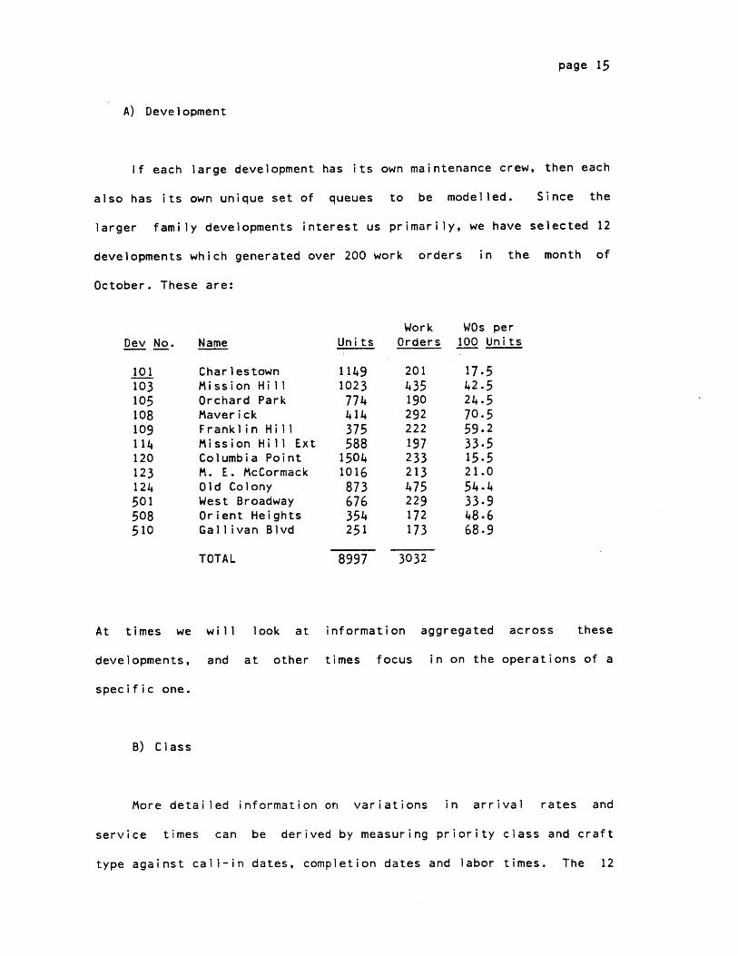
A) Development
If each large development has its own maintenance crew, then each
also has its own unique set of queues to be modelled. Since the
larger family developments interest us primarily, we have selected 12
developments which generated over 200 work orders in the month of
October. These are:
Dev No.
101103105108109114120123124501508510
Name
CharlestownMission HillOrchard ParkMaverickFranklin HillMission Hill ExtColumbia PointM. E. McCormackOld ColonyWest BroadwayOrient HeightsGallivan Blvd
TOTAL
Units
11491023
774414375588
15041016873676354251
8997
WorkOrders
201435190292222197233213475229172173
3032
WOs per100 Units
17.542.524.570.559.233.515.521.054.433.948.668.9
At times we
developments,
specific one.
will
and
look at
at other
information aggregated across these
times focus in on the operations of a
B) Class
More detai
service times
type against ca
led information on variations in arrival rates and
can be derived by measuring priority class and craft
11-in dates, completion dates and labor times. The 12

page 16
class codes are meant to describe the overall type of work order. In
one sense, orders are coded by priority (emergency, routine); in
another by special source, if any (Housing Inspection Dept, Emergency
Response Service, Court Order, LUI), and in yet another sense by
special reasons for which service might be required (lead paint,
vacancy, extraordinary, modernize, safety, security). Any work order
falls into at least one of these subcategories, but may fall into all
three. Since only one of these overlapping class codes is specified
on a work order form, however, a great deal of information can be lost
or misclassified. In the future, this information might be organized
into two unique and exhaustive categories covering priority and
source, with perhaps a third for any special characteristics not
detailed elsewhere.
For this analysis, we are primarily concerned with the priority
in which calls are serviced. Fortunately, central BHA policy has
attempted to sort each of the 12 class items by the order in which
they should be handled. Assuming that central policy has had some
effect, this allows us to retrospectively analyze all work orders by
priority. Hereafter, we will use the term "class" to refer to service
priority. The variable "class" takes on two values - emergency and
routine - with respect to which all work orders are defined. The
terms "emergency" and "routine" - used in a more comprehensive sense
than that in which they appear on a work order form - are defined to
include work orders coded as

page 17
Emergency Routine
1 emergency 4 vacancy2 lead paint 5 routine3 Housing Inspection 6 extraordinary
Department 7 modernize8 safety 12 Living Unit Inspection9 security
10 Emergency ResponseService
11 court order
This information could be used to model either the existence of one
priority-based queue for each development, or two independent queues -
one for each priority class.
C) Craft
The craft category refers to the type of craftsperson needed for
the maintenance service. According to union contracts no longer in
effect, each work order was required to be serviced by a craftsperson
of the corresponding type. This policy substantially increased the
costs and turn-around times associated with some jobs, since a
painter, for example, could not begin painting until an expensive,
licensed electrician had arrived to remove the light switch cover
plates. These rules apparently went much further than state law,
which only required that more complex tasks be performed by workers of
the corresponding specialized skill type. The fact that licensed
craftspersons are both more expensive and sometimes legally required
for certains tasks suggests that we differentiate licensed work orders
from those of other skill types. The 19 craft codes might then be
aggregated into two groups. Similar to our definition of class, the

page 18
variable "craft" takes on two values - licensed and skilled - by which
all work orders (except rare manager actions) can be defined.
Licensed Skilled
4 electrician 1 appliance10 plumber 2 auto mechanic
3 carpenter5 fireman6 glazier7 laborer8 painter9 plasterer
11 roof12 site,structure
13 steamfitter14 welder
16 exterminator17 tile setter18 bricklayer19 cement finisher
Although it can be argued that much information is lost by
grouping so many skills together, licensed work orders account for 42%
of all work orders generated, whereas any one skill type accounts for
very little. Since, for the period under study, craftspersons of a
particular type were required to service each order, one might assume
that a different queue exists for each craft. Workers in some queues
may therefore have a great deal more idle time than others. We have
ignored these distinctions here for two reasons: one is that
workorders are backlogged, usually by the hundreds, for each
development. This suggests that most workers always have calls in
queue. The other reason is that average service times do not appear to
differ dramatically by skill type. Although idle times by craft have
not been investigated here, such retrospective information could help
judge the accuracy of idle times projected by queueing models. Further
page 19
studies should certainly attempt more fine grained analyses, once the
new work order processing system is securely in place.
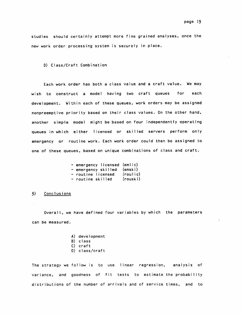
D) Class/Craft Combination
Each work order has both a class value and a craft value. We may
wish to construct a model having two craft queues for each
development. Within each of these queues, work orders may be assigned
nonpreemptive priority based on their class values. On the other hand,
another simple model might be based on four independently operating
queues in which either licensed or skilled servers perform only
emergency or routine work. Each work order could then be assigned to
one of these queues, based on unique combinations of class and craft.
- emergency licensed (emlic)- emergency skilled (emski)- routine licensed (roulic)- routine skilled (rouski)
5) Conclusions
Overall, we have defined four variables by which the parameters
can be measured.
A) developmentB) classC) craftD) class/craft
The strategy we follow is to use linear regression, analysis of
variance, and goodness of fit tests to estimate the probability
distributions of the number of arrivals and of service times, and to

page 20
see how these estimates differ with respect to the variables outlined
above. Turn-around times have been analyzed in a similar fashion to
provide a base for comparison with those which could eventually be
estimated by queueing models. Once reasonable assumptions can be made
regarding the forms taken by these distributions, parameter estimates
used as inputs to queueing models can then be easily calculated using
the same database management techniques which provide other reflective
performance measures.

page 21
CHAPTER III
ESTIMATING ARRIVAL RATES
1) Objectives
By observing arrival processes for the queues we have defined, we
can determine whether simple queueing models can be fit to these
arrivals. Here, a variety of methods are used to test whether
arrivals correspond to a Poisson process. Due to its pleasant
mathematical properties, this process has become the basis for some of
the simplest and most powerful queueing models in common use. Another
reason it is often used is that the Poisson process describes events
which occur randomly in time. Therefore, if systematic maintenance
problems are not occuring, we would expect work orders to arrive
approximately in a Poisson manner.
In the case of Poisson arrivals, scheduling operations may
clearly benefit from queueing models capable of projecting congestion.
We would therefore like to point out any Poisson arrival processes and
suggest models that may help reduce turn-around times. But since
Poisson processes describe random events, we can also use our test
results as criteria for determining whether maintenance problems are
ordinary or systematic. If arrivals are non-Poisson, then the
maintenance system would benefit from an ability to diagnose problems
by separating independent occurrences from systematic ones. We begin
with a short profile of Poisson processes, followed by an explanation
of test methods and results. An interpretation of these results can be
found at the end of this chapter.

page 22
2) The Poisson Arrival Process
The exact time at which a call for service will arrive is not
known in advance. If one were to visit a maintenance office, the time
interval between any two arrivals would be different each time. But
over a large number of observations, these interarrival times might
follow one of several classic probability distributions. If we take
one day as our time unit of analysis, we can observe a daily demand
function showing the aggregate number of work orders that arrived on a
particular day throughout the 12 high-demand developments we have
chosen. A plot of daily demand in October (fig 1), shows work orders
as a function, ) (t), of the working day on which they arrived.
Weekend days have been eliminated.
a = awos Daily demand function: figure 1
200 + work orders per day, October 1983
a
150 +a a
a a
a a aa a a a aaa a a
100 + aa
a
50 +
0 +------------------------------------------------
0 5 10 15 20
Day

page 23
Toward the end of the month, the number of arrivals appears to
drop because the data contain call-in dates only for those orders
serviced in October. Especially near the end of the month, calls are
arriving that will not be immediately serviced, and not appear in the
data until November. The mean arrival rate of these calls is 117 per
day with a standard deviation of 21. Further identification of errors
would probably raise the mean and reduce the standard deviation
somewhat.
We begin with the null hypothesis that arrivals can be modelled
as a time-homogenous Poisson process. This process has been shown
especially useful in approximating many aspects of urban service
systems. It typically applies when customers (arrivals) are drawn from
a large population, any one of which has a very small probability of
"arriving" on a given day. For general Poisson processes, the numbers
of arrivals occurring during non-overlapping time intervals are
statistically independent. If in addition the interarrival times
follow an exponential distribution, then the actual arrival pattern is
called a time-homogenous Poisson process. In any time interval, these
Poisson arrivals are said to occur "randomly" in time, and the
probability that there are exactly n work orders generated in a
particular day is given by
Pr(n/day) = Pr n = (_t) e t = 1 day
n = arrivals/day
If this equation fits the distribution of the number of arrivals as we
observe them in the data, then other well-known properties of
homogenous Poisson arrival processes will enable us to define the
system's behavior particularly well.

page 24
There are a variety of methods for testing whether this
hypothesis is true for the observed arrivals. First, we plot a
histogram showing the number of days in October on which n arrivals
occurred (fig 2).
figure 2
wos /day frequencies
90 xx 2100 'xx 2110 xxxxxxx 7120 xxx 3130 xx 2140 xx 2150 x 1160 0170 0180 Ix I
With the exception of the outlier to the right, the histogram
resembles that of a Poisson probability mass function (pmf), and
suggests we test the actual pmfs more closely for specific
developments. For each development, we then calculate means and
variances of daily arrival rates (A) by class, craft, and class/craft
combination (table 3).
Choosing development 108, a relatively busy project, we next
create table 1, showing the daily demand function. From column 1, we
can make a separate matrix (table 2) to show the number of arrivals
per day and the fraction of days on which they were observed. This is
the observed probability mass function ("frac", fig 3a). Using the
observed mean arrival rate A , we also generate a theoretical pmf
(Pr_n_arr) showing how arrivals per day would be distributed if they
corresponded perfectly to a time-homogenous Poisson process. This is
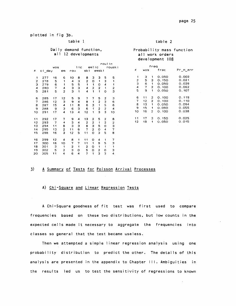
page 25
plotted in fig 3b.
table 1
Daily demand function,all 12 developments
wosci day
277 16278 5279 6280 7281 5
285 17286 12287 15288 9291 17
292 17293 7294 11295 13298 16
299 12300 18301 3302 5305 11
em
6
42
123434
74823
410
124
roul irclic emlic
rou ski emski
10 8 8 3 34 3 2 0 15 5 1 1 03 3 4 2 23 1 4 1 1
5 9 7 7 59 4 8 1 2
11 8 6 3 16 3 6 1 213 4 12 1 3
9 4 13 2 53 4 2 2 13 3 8 3 5
11 6 7 2 012 5 11 0 3
8 1 11 0 47 7 11 1 92 1 2 0 13 0 5 0 26 4 7 1 3
table 2
Probability mass functionall work ordersdevelopment 108
f reqrouski#
2345
678910
1112
5
23
366410
82378
73
34
wos
35679
1112131516
1718
13121
22
2
31
f rac
0.0500.1500.0500.1000.050
0.1000. 1000.0500.0500.100
0.1500.050
Pr_n arr
0.0030.0210.0390.0620.107
0.1190.1100.0940.0550.038
0.0250.015
3) A Summary of Tests for Poisson Arrival Processes
A) Chi-Square and Linear Regression Tests
A Chi-Square goodness of fit test was first used to compare
frequencies based on these two distributions, but low counts in the
expected cells made it necessary to aggregate the frequencies into
classes so general that the test became useless.
Then we attempted a simple linear regression analysis using one
probability distribution to predict the other. The details of this
analysis are presented in the appendix to Chapter IlM. Ambiguities in
the results led us to test the sensitivity of regressions to known
2345
678910
1112131415
1617181920

page 25a
PMF for arrivals, 108
f = frac
16.0000*10**-2
14.0000*10**-2
12.0000
figure 3a
+
+
f f
+
*10**-2
10.0000 +*10**-2
8.0000*10**-2
6.0000*10**-2
4.0000*10**-2
f f f f
+
+
+
f f
0 5 10 15 20
wos
Poisson arrivals, dev1O8
P = Pr_n arr
0. 1200 +
0. 1000 +
0.0800 +
0.0600 +
0.0400 +
0.0200 +
0.0000 +
P
figure 3b
P
P
p
P
P
P
P
P
P
P
P
0 5 10 15 20
wos

page 26
differences between probability distributions. For low arrival rates
and small sample sizes, regression results appear to underestimate
these differences. The tests are especially insensitive to differences
between cumulative distributions.
Finally, we found that non-constant variances require that a
weighted least squares approach be used. Such a regression test would
account for inhomogenous variances (just as the Chi-Square test does),
but it would also indicate how consistently and in what direction the
distributions differ. No time was available to execute a weighted
least squares regression test, however.
B) The Kolmogorov-Smirnov Test
Another method for testing the degree of agreement between a
cumulative function of observed probabilities and an hypothesized
cumulative distribution is the Kolmogorov-Smirnov (K-S) goodness of
fit test. This avoids the problem of glossing over differences
between the two distributions because it subtracts each cell in the
observed function from the corresponding cell of the expected or
hypothesized distribution, and uses the maximum resulting difference
as a test statistic, D, whose distribution in repeated sampling is
known.
D = maximumlexpected - observedi
Here, D is small under the null hypothesis that the observed
probabilities are equal to the Poisson. A large D, however, leads us
to reject the Poisson model at some chosen significance level, whose

page 27.
critical value depends on the sample size, n. Like many tests, the K-S
statistic tends to favor the null hypothesis for small sample sizes.
In our case, we want to be careful because the finer our class and
craft categories are sliced, the more the arrival processes may appear
Poisson.
We can give the non-Poisson alternative the benefit of the doubt
by choosing a significance level of a=0.20. By this decision rule, we
are willing
non-Poisson
to re
whi
Critical values
reference. But
provides us with
Table 4 in
for development
statistic D are
the regression
judges all arriv
significance.
randomly generated p
different values of
sensitive to changes
regressions has to
rather than observed
rate).
n
ject the Poisson model if our
le allowing a 20% probability
at the 0.05 level have also
either decision rule accounts for
a defin
Appendix
108.
tive answer.
III summarizes the
The distributions
observations appear
of chance error.
been provided for
recording errors or
outcomes of the K-S
used to calculate the
given in table 5 and figure 2 of the
on cumulative probability
al processes to be Poisson
distri
at any
appendix.
butions, the
reasonable
K-S
level
test
test
Like
test
of
An analysis using the K-S test to compare a series of
robabilities to a Poisson distribution based on
the mean arrival rate shows the test to be highly
in this rate. The problem faced with cumulative
some extent been overcome (here we used random
distributions to test for changes in the arrival
The interesting conclusion, however, is that the K-S statistic
also appears highly sensitive to changes in sample size. Our tests
for development 108 used a sample of 20 days and found arrivals to be
i

page 28
Poisson. But for the same sample size, the K-S test also judges a
cumulative distribution of random uniform probabilities to be Poisson,
provided we use the mean arrival rate implied by those random numbers
as our estimate of lambda in generating the expected Poisson
distribution. The same is generally true for all sample sizes less
than 60. At 60, the test discriminates well between hypothesized and
random distributions for an arrival rate of 18 work orders per day,
but not for 12. It is only for sample sizes of at least 100, however,
that it appears clearly useful for testing hypotheses throughout the
range of the arrival rates in our observed distributions. The test is
therefore inadequate for estimating arrival distributions from monthly
samples. The results of these investigations are presented in tables 6
and 7 of Appendix Ill.
C) Measures of Central Tendency Across Developments
Finally, Poisson arrival processes also have the property that
the mean number of Poisson events occurring in a given time period is
precisely equal to the variance. The means and variances of daily
arrival rates are given in tables 3a and 3b by class, craft,
class/craft and development. If the means and variances for any
development are equal, this does not prove the arrivals are Poisson,
but very different means and variances would suggest that they are
not.
Using data from all 12 developments, linear regressions were run
to test how well the observed means predict the variances. While this
masks the differences between any two developments, it permits us to
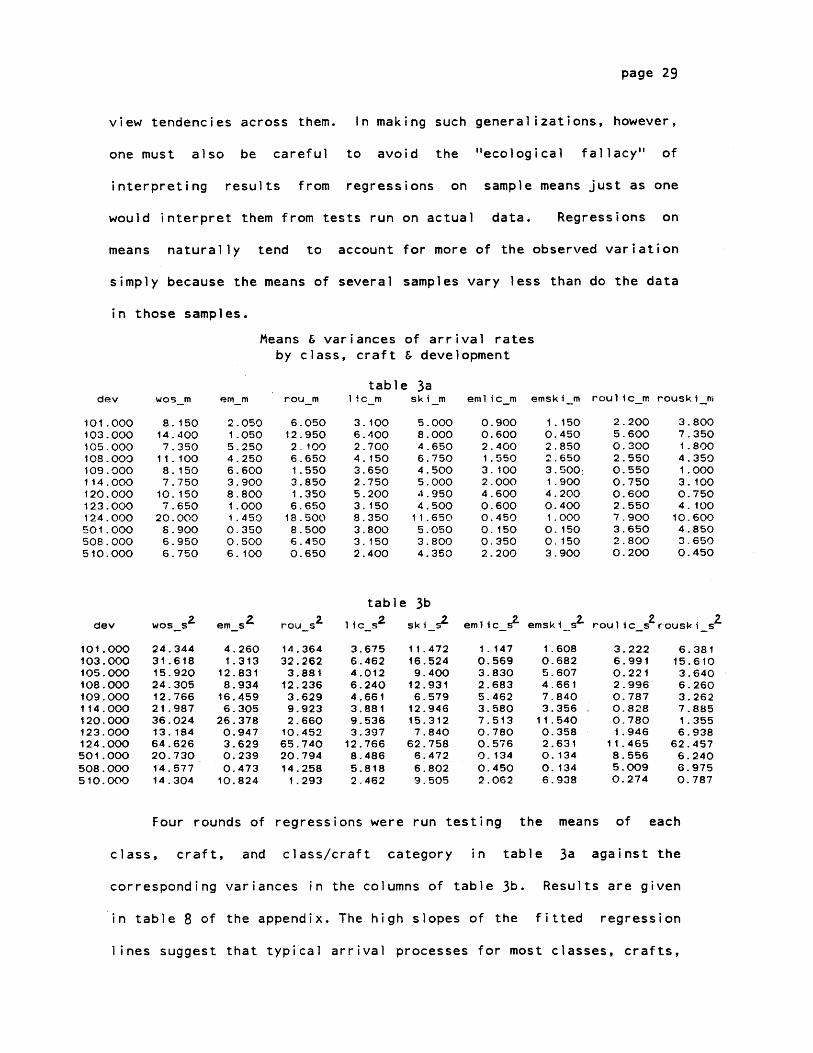
page 29
view tendencies across them. In making such generalizations, however,
one must also be careful to avoid the "ecological fallacy" of
interpreting results from regressions on sample means just as one
would interpret them from tests run on actual data. Regressions on
means naturally tend to account for more of the observed variation
simply because the means of several samples vary less than do the data
in those samples.
Means & variances of arrival ratesby class, craft & development
wos-m emm
8.15014.4007.350
11.1008.1507.750
10.1507.650
20.000S.9006.9506.750
2.0501.0505.2504.2506.6003.9008.8001.0001.4500.3500.5006.100
table 3arou m lic_m ski m
6.05012.9502.1006.6501.5503.8501.3506.650
18.5008.5006.4500.650
3.1006.4002.7004.1503.6502.7505.2003.1508.3503.8003.1502.400
5.0008.0004.6506.7504.5005.0004.9504.50011.6505.0503.8004.350
emlic m emskim roulicm rouski m
0.9000.6002.4001.5503.1002.0004.6000.6000.4500.1500.3502.200
1.1500.4502.8502.6503.500,1.9004.2000.4001.0000.1500.1503.900
2.2005.6000.3002.5500.5500.7500.6002.5507.9003.6502.8000.200
3.8007.3501.8004.3501.0003.1000.7504.100
10.6004.8503.6500.450
table 3b
wossA em-s A rousa 1i cs2 sk i-s2
24.34431.61815.92024.30512.76621.98736.02413.18464.62620.73014.57714.304
4.2601.313
12.8318.934
16.4596.305
26.3780.9473.6290.2390.473
10.824
14.36432.262
3.88112.2363.6299.9232.660
10.45265.74020.79414.258
1.293
3.6756.4624.0126.2404.6613.88 19.5363.397
12.7668.4865.8182.462
11.47216.5249.400
12.9316.579
12.94615.3127.840
62.7586.4726.8029.505
eml i c_sA emsk ils2 roul i c sz rousk i s
1.1470.5693.8302.6835.4623.5807.5130.7800.5760.1340.4502.062
1.6080.6825.6074.6617.8403.356
11. 5400.3582.6310.134
0.1346.938
3.2226.9910.2212.9960.7870.8280.7801.946
11.4658.5565.0090.274
6.38115.6103.6406.2603.2627.8851.3556.938
62.4576.2406.9750.787
Four rounds of regressions were run testing the means of each
class, craft, and class/craft category in table 3a against the
corresponding variances in the columns of table 3b. Results are given
in table 8 of the appendix. The high slopes of the fitted regression
lines suggest that typical arrival processes for most classes, crafts,
dev
101.000103.000105.000108.000109.000114.000120.000123.000124.000501.000508.000510.000
dev
101.000103.000105.000108.000109.000114.000120.000123.000124.000501.000508.000510.000
page 30
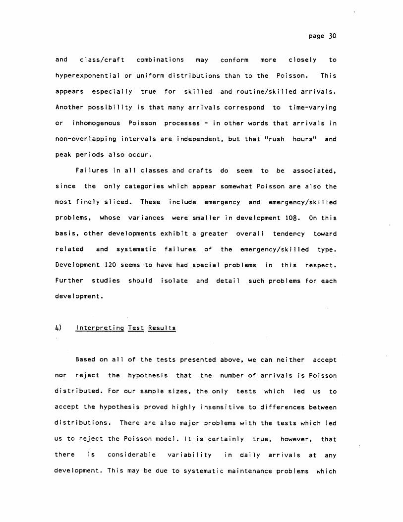
and class/craft combinations may conform more closely to
hyperexponential or uniform distributions than to the Poisson. This
appears especially true for skilled and routine/skilled arrivals.
Another possibility is that many arrivals correspond to time-varying
or inhomogenous Poisson processes - in other words that arrivals in
non-overlapping intervals are independent, but that "rush hours" and
peak periods also occur.
Failures in all classes and crafts do seem to be associated,
since the only categories which appear somewhat Poisson are also the
most finely sliced. These include emergency and emergency/skilled
problems, whose variances were smaller in development 108. On this
basis, other developments exhibit a greater overall tendency toward
related and systematic failures of the emergency/skilled type.
Development 120 seems to have had special problems in this respect.
Further studies should isolate and detail such problems for each
development.
4) Interpreting Test Results
Based on all of the tests presented above, we can neither accept
nor reject the hypothesis that the number of arrivals is Poisson
distributed. For our sample sizes, the only tests which led us to
accept the hypothesis proved highly insensitive to differences between
distributions. There are also major problems with the tests which led
us to reject the Poisson model. It is certainly true, however, that
there is considerable variability in daily arrivals at any
development. This may be due to systematic maintenance problems which
page 31
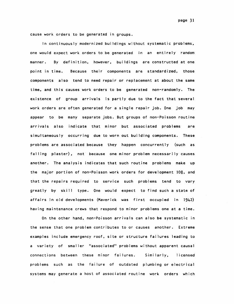
cause work orders to be generated in groups.
In continuously modernized buildings without systematic problems,
one would expect work orders to be generated in an entirely random
manner. By definition, however, buildings are constructed at one
point in time. Because their components are standardized, those
components also tend to need repair or replacement at about the same
time, and this causes work orders to be generated non-randomly. The
existence of group arrivals is partly due to the fact that several
work orders are often generated for a single repair job. One job may
appear to be many separate jobs. But groups of non-Poisson routine
arrivals also indicate that minor
simultaneously occurring due to worr
problems are associated because they
falling plaster), not because one
another. The analysis indicates that
the major portion of non-Poisson work
that the repairs required to service
greatly by skill type. One would
affairs in old developments (Maverick
having maintenance crews that respond
On the other hand, non-Poisson ar
the sense that one problem contributes
examples include emergency roof, site
a variety of smaller "associated"
connections between these minor fa
but associated problems are
out building components. These
happen concurrently (such as
minor problem necessarily causes
such routine problems make up
orders for development 108, and
such problems tend to vary
expect to find such a state of
was first occupied in 1942)
to minor problems one at a time.
rivals can also be systematic in
to or causes another. Extreme
or structure failures leading to
problems without apparent causal
iilures. Similarly, licensed
problems such as the failure of outdated plumbing or electrical
systems may generate a host of associated routine work orders which

page 32
appear unrelated. Such bunches of routine work orders could well
indicate that more serious problems are about to happen, and that
there are major problems underlying these minor failures.
The fact that we are unable to assume arrivals to be Poisson
distributed does not help us to construct simple and accurate queueing
models. But it does suggest that the more serious (and interesting)
maintenance problems involve precisely those work orders which do not
arrive in a Poisson manner. We can use this fact to help us identify
possible systematic failures.
It is important that we not confuse service priorities with the
degree to which a problem may result from systematic failures.
Emergency work orders
serious systems pro
emergencies can be
occurrences. If mos
view work orders a
systematically gener
these problems are th
as systematically,
which are likely to
are not ne :essar i 1 y the main indicators of
blems. While they require priority service, these
the result of either related or isolated
t arrival categories are non-Poisson, we should
s symptoms of a maintenance process that
ates certain types of problems. By definition,
e cumulative effects of systematic neglect. Just
therefore, we must define the underlying failures
be causing different "bunches" of associated
problems, whether they be emergency or routine, licensed or skilled.

page 33
5) Diagnosing Systems Failures
A) The Bottom-Up Approach
A method for identifying system failures can be briefly outlined
as follows. One first identifies a specific bunch of problems that are
regularly occurring. Again, these problems are "associated" because
they are of the same type, rather than because they necessarily cause
each other. Only rarely will bunches will be observable in the space
of one day, since failures may not create symptoms all at once. It is
more likely that neglected systems will be identified by isolating
"bunches" that form over periods of several weeks or even months.
Each bunch can then be viewed as one element in a hypothetical
set of such symptoms. At the disaggregated level, these bunches may
appear unrelated to other elements of the same set. Indeed, workers
may fail to notice (or to record) the existence of a "set" of
problems, since they tend to service work orders of a particular type.
But these diverse elements may in fact be related through systems
failures. The bottom-up approach asks what possible systems failures
are implied by the diverse non-random problems we observe in work
order data.
B) The Top-Down Approach
The same method for identifying systems failures can be seen from
another perspective. First, a list of possible systems failures is
created. From these, one can generate hypothetical sets of problems

page 34
which could follow from such failures. Each set implies a
corresponding systems failure, and each element in a set constitutes a
symptom or bunch of associated work orders which would appear in the
data if the related systems problem may be occurring. Any systems
problem may therefore imply a variety of possible symptoms, not all of
which would necessarily manifest themselves in the event such failures
exist. From the appearance of a few symptoms or bunches, one could
then diagnose possible failures. Furthermore, if a given underlying
problem is suspected, one should be able to anticipate other bunches
of work orders that may "happen", since these are simply the remaining
elements of the system's set. The diagnosis is complicated somewhat,
however, by the fact that a given symptom may imply a variety of
systems failures, and therefore belong to several sets at once. This
should be clear from the diagram (figure 4) on the following page.
The term "systems failures" should not conjure images of
exploding boilers, flooded corridors and collapsing ruins, however.
The reason we need a method for diagnosing them is precisely that they
may otherwise go unrecognized. The method outlined here is essentially
meant to be used for analyzing neglected or undermaintained building
systems, since they may be hidden behind work orders which appear to
workers as isolated events. Rather than cataloguing every imaginable
system, the bottom-up approach should be used initially to identify
those "most neglected" systems for which system sets should be
constructed. The detailed task code scheme provided by the new work
order processing system should be quite useful for this.

Figure 4. DIAGNOSING SYSTEMS FAILURE3 FROM TASK CODE DATA.
Y5TE MS FAIL
5YMPTOM 5E
5YMPTOMS.THERE MAY NOAPPARE NT RELATIONBE TWEEN BUNCHUA
VwCo
'-'3
C)

page 35
6) Summary & Conclusions
Our analysis of arrival rates therefore indicates that
1) A variety of non-random problems are occurri-ng;
2) These failures are associated but are not necessarily
causing other failures to occur;
3) Underlying systems failures which may be causing diverse
types of non-random problems are not always recognized
in the field or by monthly reviews of work order data, but
4) they can be identified by constructing sets of
symptoms which appear in the data as bunches of
associated work orders. These sets can then be used to
structure monthly reviews.
5) Data should be organized by the new work order processing
system so that work orders can be sorted into bunches
by task code, and
6) Living Unit Inspection data should be structured to further
identify such problems by classifying the condition of
components common to many apartments.
Finally, waiting time consequences for most arrival processes
might not be approximated with acceptable accuracy by simple
Poisson-based queueing models. It appears quite likely that work order
arrivals are uniformly distributed, although other models may apply.
Conversely, however, the degree to which arrival distributions change
over time into Poisson processes may be used as a measure for
evaluating improvements in building conditions. As systematic and
associated failures are identified and serviced, one would expect
page 36
arrivals of subsequent work orders to
distributions. In turn, this would enable
to be made from simple queueing models.
modified and expanded LUI program and the
proposed work order processing system seem
general direction.
more closely follow Poisson
more accurate projections
From this perspective, the
task code scheme of the
to be oriented in the right

page 37
CHAPTER IV
SERVICE TIMES
1) The Poisson Service Process
Service times measure the time actually spent performing
maintenance tasks. These are usually very small in comparison with
the time customers spend in queue (by far the largest component of
turn-around times), but they play an important role in determining the
lengths of those queues.
<-----------turn -around time---------
--------- waiting time--------' +
cal-ndays.horcall-in completiondate. da t.
The strategy for estimating service time distributions is similar
to the one we used for analyzing arrivals. There, we tested to see if
the interarrival times follow an exponential distribution, which is
equivalent to saying that the arrival rates could be modelled by a
Poisson probability mass function. We assumed the interarrival times
to be independent, and tested this assumption by measuring events per
unit time with the aid of the pmf.
For a Poisson service process, however, it is the time between
service completions (the service times) that are independent and which
follow an exponential distribution. Instead of measuring probability
distributions of events in a fixed time interval, we now measure
probabilities that the time interval needed for an event to occur will

page 38
assume some value. Therefore, we approximate a Poisson service
process by calculating expected probabilities using the probability
density function (pdf) for a negative exponential distribution, which
is given by-ut
Pr{ste (t,t+dt)} = ue dt t > 0
This is the set of probabilities that a service completion occurs in
any given time interval, or, equivalently, the probabilities that
service times are of a given duration.
As A stood for the mean arrival rate of calls per day, here u
equals the mean service rate per hour and t is the independent random
variable describing the number of hours. Mean service times calculated
from the data, however, are given by 1/u. Tables 4a and 4b present
means and standard deviations for these service times by development,
class, craft, and class-craft combination.
(1)
Taking the inverse of the observed mean service time (1/u) for
development 108 transforms it to a mean service rate (u), which can be
substituted into the formula for the negative exponential
distribution. Integrating the areas under the curve for each service
rate then gives the expected probability density function for our
hypothesized Poisson service process.
In table 1, development 108 work orders have been sorted by
service times for all class and craft categories. The aggregate column
(1)For further reference, table 1 in Appendix IV shows the actual number
of workorders in each service time category by class, craft, andclass-craft. These figures are aggregated across all 12 developments.
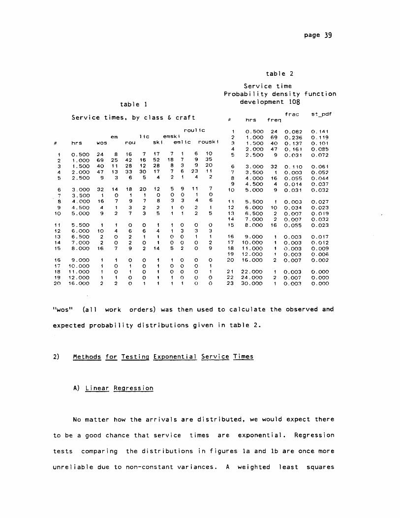
table 2
Service timeProbability density
development 108
Service times, by class & craft # hrs freqfrac stpdf
# hrs wos
12345
67
910
1112131415
1617181920
0.5001.0001.5002.0002.500
3.0003.5004.0004.5005.000
5.5006.0006.5007.0008.000
9.00010.00011.00012.00016.000
246940479
321
1649
1102216
11
2
roul icem lic emski
rou ski emlic rouski
82511133
140712
14007
100i2
"wos" (all work
164228336
18
937
06229
0
00
71612305
201723
06102
0000O1
175228174
1208
25
4411
14
718872
503
11
110
5
1
11
699
234
11
4
22
03100
0000O)
103520112
706
5
03129
0110O0
1 0.5002 1.0003 1.5004 2.0005 2.500
6 3.0007 3.5008 4.0009 4.500
10 5.000
1112131415
1617181920
212223
5.5006.0006.5007.0008.000
9.00010.00011.00012.00016.000
22.00024.00030.000
246940479
321
1649
10
2216
2
12
1
0.0820.2360. 1370. 1610.031
0.1100.0030.0550.0140.031
0.0030.0340.0070.0070.055
0.0030.0030.0030.0030.007
0.0030.0070.003
0.141
0.1190.1010.0850.072
0.0610.0520.0440.0370.032
0.0270.0230.0190.0320.023
0.0170.0120.0090.0060.002
0.0000.0000.000
orders) was then used to calculate the observed and
expected probability distributions given in table 2.
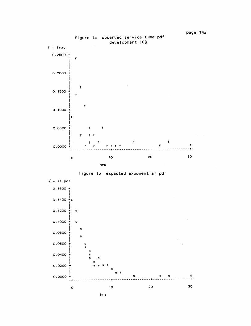
2) Methods for Testing Exponential Service Times
A) Linear Regression
No matter how the arrivals are distributed, we would expect there
to be a good chance that service times are exponential. Regression
tests comparing the distributions in figures la and lb are once more
unreliable due to non-constant variances. A weighted least squares
page 39
table 1
function
page 39a
figure la observed service time pdfdevelopment 108
f = frac
0.2500 +
0.2000 +
. +0.1500 +
0. 1000 +
if
0.0500 + f f
I f f f0.0000 4 f f f f f f f f
-- - - - --- - - - - - - -----------------------------
o 10 20 30
hrs
figure 1b expected exponential pdf
s = st_pdf
0. 1600 +
0. 1400 +s
0.1200 + s
0.1000+ S
I S
0.0800 +i S
0.0600 + S
0.0400 + SS S
S
0.0200 + S S S S
ssi ~ s S
0.0000 + s S S S0-----------------------------
0 10 20 30
hrs

page 40
approach is again necessary if a regression test is to be used.
Details of simple regression results are given in Appendix IV.
B) The Kolmoqorov-Smirnov Test
Service time distributions can be reviewed, however, using the
Kolmogorov-Smirnov goodness of fit test. We avoid the problem of
small sample size here, because our sample is the number of work
orders rather than the number of days. Results of the tests are given
in table 3, and the calculations are in table 4 of the appendix. For
all large sample sizes, the K-S statistic leads us to reject the
exponential hypothesis.
C) Measures of Central Tendency
For arrival processes, we used the fact that Poisson means and
variances are precisely equal as a final test of the degree to which
the observed arrivals in development 108 are representative of those
in the other 11. With the exception of emergency, emergency/licensed
and routine/licensed jobs, we found the variances to be much higher
than the means, - suggesting that uniform or hyperexponential
distributions may be more accurate predictors of some arrival
processes.
We can follow an analogous strategy as a final test for
exponential service times. For development 108, a K-S test has
provided reasonable evidence that service times are not exponentially
distributed. A comparison of the means and variances may enable us to

Kolmogorov-Smirnov Goodness of Fit Testfor
Observed vs. Expected Poisson Service Time Distributions, by Class & Craft,Development 108
Ho: observed = exponentialH1: observed i exponential
Class/CraftCategory
D stat.Sample size
n
Critical Value
a = .20 a = .05
All workorders
Emergency
Routine
Licensed
Skilled
Emlic
Emski
Roulic
Rouski
.177
.135
.189
.193
.216
.173
.185
.200
292
100
188
114
174
37
62
76
.063 .080
.107
.078
.100
.081
.175
.136
.123
.136
.099
.127
.103
.223
.173
.160
reject Ho
accept at .05
reject
reject
reject
accept at .20
reject
reject
.102 .130 reject
Decision
-h0
00
D 0
0
M 0'
0 <
r+
CD
00
a
a--,
CL
0
r+
0-r-
0W)
.228 109

page 41
table 4
Means & standard deviations of service timesby class, craft & development
wos_m em m rou m lic-m skim emlicm emskim roulicm rouski m
2.5123.3973.0953.0094.0273.4292.4704.1852.2203.7533.9652. 173
2.3533.0833.1653.0203.1483.8681.7845.8262.2166.9441.9172.083
2.5743.4562.9303.0378.2633.0205.8853.9872.2243.6374.1192.795
1. 9692.8903.4672.8423.1004.0341.8213.1221.7902.4782.1342.636
2.8913.8562.9223.0894.6293.1763.1254.9062.5334.6205.2521 .934
2.2273.0153.6133.2572.7044.2621.8254.0772.500
14.2501.7782.716
2.4483.2352.8672.8633.4503.5571.7398.1002.0801.2502.3331.760
1.8732.8222.3572.6515.1073.4381.7942.9521.7451.9242. 1852.125
3.0514.0343.0103.271
10. 1042.9429.0454.6322.5864.7525.3423.179
dev wos_S
101.000103.000105.000108.000109.000114.000120.000123.000124.000501.000508.000510.000
3.9074.6633.9723.5756.8435.5165.2815.3223.2087.7577.2012.018
em s rou_s lic_s sk i_s emlic_s emsk is roulic s rouski s
3.0424.2044.4342.9785.2045.8031.9645.6802.219
11.6901. 1651.814
4.1814.8032.6233.890
11. 1465.229
11.6745.2583.2827.5797.4393.062
1.3862.9055.7312.8432.5993.5432.1842.5622.1024.0092.3042.191
4.9215.7392.8404.0068.4556.1487.1126.4753.7899.3748.9951.888
1.8174.0786.0632.8762.0193.7682.2672.2162.374
15.3541.1212.232
3.7454.3782.9213.0726.4787.0331.5917.8842.1780.6451.4431.469
1.1912.6171.6512.8414.0632.8921.6682.5962.0831 .2282.4301 .959
5.2826.1042.7344.496
13.4515.565
14.8486.3063.9199.5249.1153.555
tentatively extend these conclusions to other developments.. The
method is similar to the one employed for arrivals, but not identical,
because service time distributions have been modelled using a pdf
rather than a pmf. For a Poisson service process, the mean service
time is 1/u and the variance is 1/u2 . Therefore, the standard
deviation (rather than the variance) is precisely equal to the mean,
since
To test how closely the values in the columns of table 4a match those
of table 4b, we use the same method as in comparing the means and
dev
101.000103.000105.000108.000109.000114.000120.000123.000124.000501.000508.000510.000

page 42
variances of arrival rates. A first glance suggests that the means in
each class and craft category are fairly close to their corresponding
standard deviations. Results of the regressions are presented in table
5 of Appendix IV.
The r-square terms are uniformly higher than tests run for
development 108 alone, as one would expect from regressions run on
sample means. The slopes of lines fit by the regressions, however, are
fairly close to one. Means and standard deviations are furthest from
matching for skilled jobs, but we expect more variation here, due to
the greater variety of job types in this category.
3) Interpretation & Conclusions
If we had found service times to be exponential, then the time
remaining until the next service completion would be independent of
the particular time at which we choose to view the service process. It
would also be independent of the type of work order previously
serviced. This is the Markov or "no memory" property of Poisson
service processes. Exponential service times would therefore indicate
that different types of repairs are being done within any class or
craft category, since these repairs are taking different amounts of
time to service. Such repairs would be unassociated and not
consequences of systems failures. We might then expect any categories
of Poisson arrivals to correspond to exponential service time
categories.
But matters are more complicated than this. Two unrelated jobs
may take the same time to be serviced, just as two associated jobs may

page 43
have different service times. The fact that several workers may be
needed to handle a given problem indicates that some jobs are
interdependent and that the service times for these jobs are mixed
together. Service interdependency means that queues can form on queues
as some tasks are delayed in mid-service until help arrives from
workers of another specialized skill needed to complete the task.
Furthermore, this additional server may himself leave
standing in a second queue while he is servicing minor
first. Given this interdependent operating method, Pois
and service processes would not necessarily correspond.
Recording is another difficulty. "Bumps" appear in
time distributions for jobs that take convenient time
service (4 hours, 8 hours, 16 hours, 40 hours). These
contain rounding errors and thus not correspond to
durations of particular types of service. Rounding errors
other jobs
tasks
son
in
arr
the
val
the service
intervals to
times may
theoretical
for the many
short service times may be especially large relative to theoretical
service times.
Despite these recording errors, systematic maintenance problems
and job interdependency appear to be more important reasons we observe
no mathematically neat distribution underlying service times.
There is a more important explanation, however, for the observed
service time distributions than all those we have discussed so far.
It is based on the fact that means and standard deviations do not
merely correspond within class and craft categories; these measures of
central tendency are also remarkably similar across those categories.
Service times are on the whole much more regular or homogenous than
the arrival rates we observed. This is an indication that maintenance

page 44
crews are responding to calls by cosmetically treating diverse
problems in similar ways.
Rather than undertaking projects aimed at the long term
improvement of conditions, crews may be so used to operating in a
"reactive mode" that the solutions they prescribe and apply merely
alleviate symptoms in the short run where they should be diagnosing
and treating underlying failures. Crews appear overworked and
yet this may indicate a need to reorganize service
priorities and methods, rather
Unit Inspection program seems o
modes of operation. But it
concentrate their efforts so he
are unable to devote attention
Systematic problems often
reaction. A structure therefore
avoids the tendency merely
encourages workers to initiate
than to expand personnel. The Living
ne way to begin to explore "initiatory"
is important that these inspections not
avily on apartment interiors that they
to more global buildings systems.
cannot be resolved through piecemeal
must be found for the LUI program that
to react to scheduling routines, and
diagnoses. Because of their diverse
nature, many systematic problems will not be isolated through data
analysis, but can only be discovered in the field by craftspersons and
supervisors who operate diagnostically.
The method for constructing system arrival sets outlined in the
previous chapter can also be used to create corresponding service
solution sets and to define system-oriented schedules that coordinate
the diverse maintenance operations needed to upgrade undermaintained
systems.
understaffed,
page 45
CHAPTER VTURN-AROUND TIMES
1) Uses for the Data
For all jobs serviced in October, turn-around time (tat) data
indicate how many working days each order spent in the queueing system
from the day on which the request was called in through the day
service was completed. Weekend days and holidays have been eliminated
so that turn-around times more accurately reflect the actual working
time required for the system to respond to demand. Of course, from
tenants' point of view, weekend days are included in the time they
must wait for service. But the inclusion of weekend days also
exaggerates working day turn-around times by as much as 30 days for
calls which are backlogged several months. Eliminating non-working
days may therefore help us to better understand the relationship
between actual system operations and turn-around times.
Had we been able to conclude in the previous chapter that arrival
and service time distributions follow a Poisson process, then we could
have modelled maintenance operations for development 108 as an M/M/n
queueing system. This would have allowed us to compare hypothetical
operating policies and to draw relatively specific conclusions, such
as: "For policy x, 90% of emergency work orders will be serviced
within 24 hours"; or "The expected average waiting time for routine
calls is 5.5 days"; or "There is an 80% probability
or less will be in queue at time t".
that w work orders
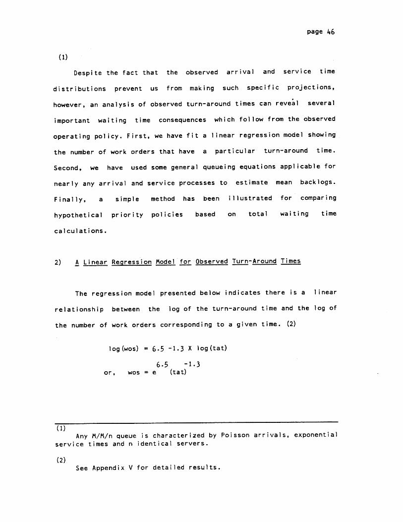
page 46
(1)
Despite the fact that the observed arrival and service time
distributions prevent us from making such specific projections,
however, an analysis of observed turn-around times can reveal several
important waiting time consequences which follow from the observed
operating policy. First, we have fit a linear regression model showing
the number of work orders that have a particular turn-around time.
Second, we have used some general queueing equations applicable for
nearly any arrival and service processes to estimate mean backlogs.
Finally, a simple method has been illustrated for comparing
hypothetical priority policies based on total waiting time
calculations.
2) A Linear Regression Model for Observed Turn-Around Times
The regression model presented below indicates there is a linear
relationship between the log of the turn-around time and the log of
the number of work orders corresponding to a given time. (2)
log(wos) = 6.5 -1.3 X log(tat)
6.5 -1.3or, wos = e (tat)
(1)Any M/M/n queue is characterized by Poisson arrivals, exponential
service times and n identical servers.
(2)See Appendix V for detailed results.

page 47
This equation defines the number of work orders which spent t days in
the queueing system. Because both variables in the regression
equation have been logged, the resulting linear relationship can be
interpreted as a constant elasticity. In other words, a 1% change in
the number of work orders is accompanied by a 1% change in the length
of the turn-around time.
This equation can be used to compare October turn-around times
with those following from recent operations changes. However,
reductions in routine times following these changes will be
exaggerated by the fact that routine work orders are now generated
solely by the Living Unit Inspection program.
figure 1
Fitted and actual relationshipsbetween
work orders and turn-around time
f = fitted
1 = Intat
5 +
4 +f1 f f f' f1 1 f fII
f 11f11fI f f f 1
3 + f fif 1fl1i
f f 1
fif
2+ fiff I
f 1
f
0 +1-------- +------------------- +-------------------- +--------------------
0 2 4 6 8
Inwos

page 48
Figure 1 shows how closely the fitted regression line corresponds
to the data. The equation also holds for all classes and crafts of
work orders (see Appendix V) and suggests that over all developments
there is no appreciable difference between emergency and routine
turn-around times.
In a truly priority-based queueing system, newly arriving routine
calls would not be serviced until all emergencies had been handled.
The data, however, are more representative of a maintenance system in
which separate queues exist for emergency and routine work orders. If
for example one crew services only emergencies, while another handles
only routine calls, then both queues may be equally congested.
In addition, BHA staff have noted the difficulty of comparing
mean turn-around times in any one development or month with those of
another. The difficulty arises because those crews operating quickly
in any month (or receiving fewer calls) will begin to service
backlogged orders toward the end of that month. Because these orders
have been in the system a long time, the crew's mean turn-around time
will be driven upward by the act of servicing them. Reliance on such
statistics for comparing month-to-month performance creates incentives
to "wish away" or purge backlogged orders.
The resulting confusion (table 1) is not due to the structure of
the data, however, but rather to the operating method in use. By this
method, work orders which have already spent a month in queue are sent
back to the end of the line, where they are ignored until the system
is uncongested enough to deal with them. Service priority is above all
given to work orders arriving in the current month, rather than to
emergency calls per se. Only if older work orders cease to be sent to
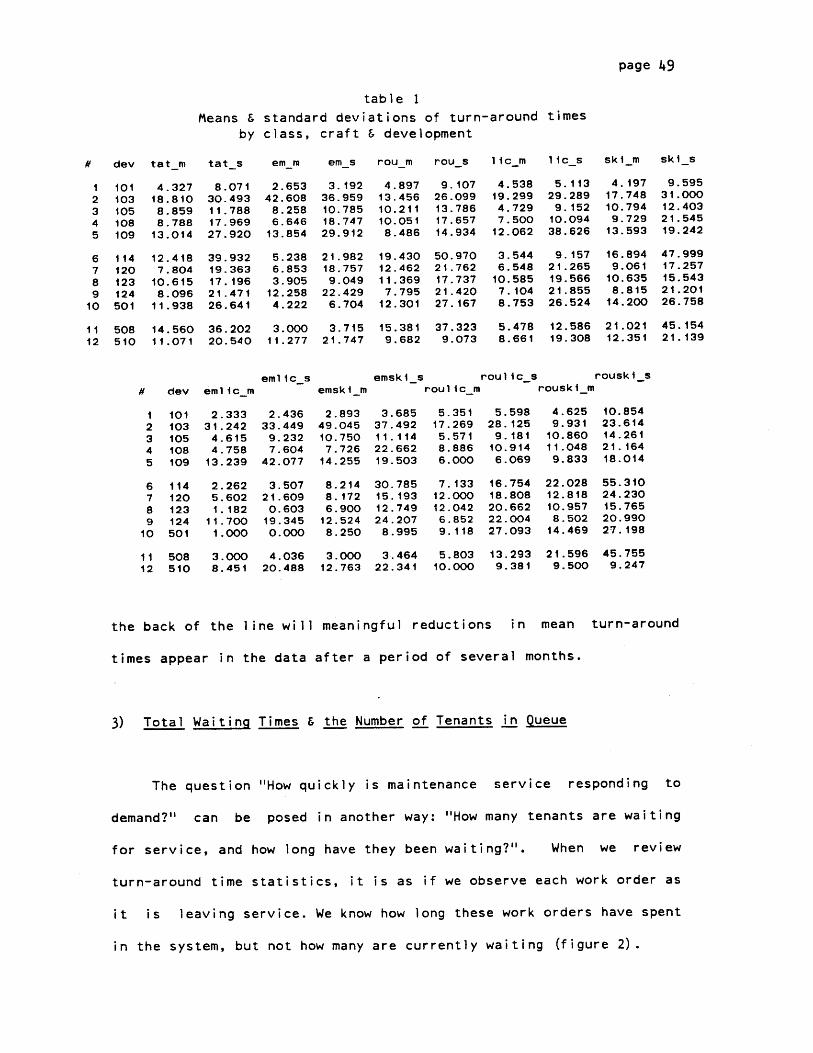
page 49
table 1Means & standard deviations of turn-around times
by class, craft & development
# dev tat-m
12345
6789
10
101103105108109
114120123124501
4.32718.8108.8598.788
13.014
12.4 187.804
10.6158.096
11.938
tat_s
8.07130.49311.78817.96927.920
39.93219.36317.19621.47126.641
em-m em-s rou-m
2.65342.6088.2586.646
13.854
5.2386.8533.905
12.2584.222
3.19236.95910.78518.74729.912
21.98218.7579.049
22.4296.704
4.89713.45610.21110.0518.486
19.43012.46211.3697.795
12.301
rou-s lic-m lic-s ski-m ski-s
9.10726.09913.78617.65714.934
50.9702 1 . 76217.73721.42027.167
4.53819.2994.7297.500
12.062
3.5446.548
10.5857.1048.753
5.11329.2899.152
10.09438.626
9.15721.26519.56621.85526.524
4. 19717.74810. 7949.729
13.593
16.8949.061
10.6358.815
14.200
9.59531.00012.40321.54519.242
47.99917.25715.54321.20126.758
11 508 14.560 36.202 3.000 3.715 15.381 37.323
12 510 11.071 20.540 11.277 21.747 9.682 9.0735.478 12.586 21.021 45.1548.661 19.308 12.351 21.139
# dev em1 i c_m
I 1012 1033 1054 1085 109
6 1147 1208 1239 124
10 501
11 50812 510
2.33331.2424.6154.758
13.239
2.2625.6021. 182
11.7001.000
emlic_s
2.43633.4499.2327.604
42.077
3.50721.6090.603
19.3450.000
emsk I_m
2.89349.04510.7507.726
14.255
8.2148.1726.900
12.5248.250
emskis
3.68537.49211.11422.66219.503
30.78515.19312.74924.207
8.995
roul ic_m
5.35117.2695.5718.8866.000
7.13312.00012.0426.8529.118
roulic_5s
5.59828.125
9.18110.9146.069
16.75418. 80820.66222.00427.093
rousk i _m
4.6259.931
10.86011.0489.833
22.02812. 81810.9578.502
14.469
rouski s
10.85423.61414.26121.16418.014
55.31024.23015.76520.99027.198
3.000 4.036 3.000 3.464 5.803 13.293 21.596 45.755
8.451 20.488 12.763 22.341 10.000 9.381 9.500 9.247
the back of the line will meaningful reductions in mean turn-around
times appear in the data after a period of several months.
3) Total Waiting Times & the Number of Tenants in Oueue
The question "How quickly is maintenance service responding to
demand?" can be posed in another way: "How many tenants are waiting
for service, and how long have they been waiting?". When we review
turn-around time statistics, it is as if we observe each work order as
it is leaving service. We know how long these work orders have spent
in the system, but not how many are currently waiting (figure 2).

page 50
f i gure 2
A General Queueing 5yst em.
QueuesX X X X x X
xx x x x x x
I number in queueI waiting time
x
ser vice facilityserver i
3
( r-lxri
| | number in service1 i service time j
Fortunately, BHA Monthly Management Reports contain estimates of
the number of outstanding work orders by development. The size of
these backlogs does not change dramatically from one month to the next
and suggests that the system is approximately in a steady state. This
means that the number of tenants in the queueing system remains
roughly constant over time. A general relationship in queueing theory
known as "Little's formula" can be used to compare BHA backlog
estimates with those expected from a steady state system with the same
arrival and turn-around time statistics.
Little's formula
meanarri valrate
completedwork
orders01
L = 2 W

page 51
Here L is the expected steady state number of work orders in the
queueing system, - is the mean arrival rate (Poisson or not), and W
is the expected steady state time in the system for a given work
order, or the mean turn-around time.
Tenants in
Mean Tat
W
4.3318.818.868.79
13.01
12.427.8010.628.10
11.94
14.5611.07
the Queueing
Estimatew/Little'sFormula
L
352716598106
967981
162106
10175
System
BHA Estimate
352671154140219
21165
284627294
14377
Calculations of L based on Little's formula underestimate the
number of outstanding work orders as given in Monthly Management
Reports (table 2). More tenants are actually waiting than we would
expect to find. The problem is not that mean turn-around times have
been skewed upward by the servicing of backlogged orders in any month,
but rather that they fail to reflect the higher turn-around times
associated with those orders still unserviced. Real mean turn-around
times are higher than they appear in the data, and therefore actual
backlogs are larger than those estimated by Little's formula.
One reason actual turn-around times are so long (and backlogs so
table 2
Dev
101103105108109
114120123124501
508510
Estimated
ArrivalRate
;k x
8.1514.407.3511.108.15
7.7510-157.65
20.008.90
6.956.75

page 52
large) is that some older work orders are repeatedly being sent to the
back of the line. But this may not account for all of the difference
between L and the BHA estimate. Another reason may be that many repair
jobs involve several work orders (and servers), since more than one
skill may be required to perform the repair. For such interdependent
jobs, servers in one queue may be kept waiting for related or
prerequisite orders to be serviced by those in another. There is also
then a queueing process operating for these servers, many of whom may
be kept "busy" waiting in the queue.
For a steady state queueing system,
/02 <1 k = number of serversku
must be true. If/ (rho) is greater than one, there will be no
steady state, since calls are arriving faster than servers are
theoretically able to handle them. In "unstable" queues of this type,
even minor increases in the arrival rate lead to major congestion.
Because wild fluctuations in backlog are not occurring, we assume that
a steady state exists and that the number of servers is theoretically
adequate. A good deal of the actual backlog may therefore be due to
the existence of tandem or interdependent queues. In order for
turn-around times to be reduced, the interdependencies leading to
"server queueing" also must be reduced. The recent reclassification of
many tasks as "neutral" should certainly improve the situation, but
the "neutral" job category may have to be expanded to include a wider
range of tasks. It is important to know which tasks contribute most

page 53
heavily to queue interdependency. These will appear as "bunches" of
work orders in monthly data.
We have seen how the operating policy with respect to backlogs
and the delays due to interdependent servicing account for the low
estimate of'L given by Little's formula. In addition, the fact that
several work orders may be generated for one repair job means that BHA
backlog figures provide too high an estimate of the steady state
number of apartments (tenants) in the queueing system. If only one
work order were generated per job, and if backlog policy were changed
and queue interdependency eliminated, then Little's formula should
provide an accurate estimate of those in the system. To find the
steady state number in queue (Lq), we subtract the number in service
on any day (A/u) from L. Here u has been transformed to a daily
service rate.
Lq = kWq = Z(W - _I) - AW - _ L - _u u u
In a one-order-per-job operating system, Lq would also equal the
steady state number of outstanding work orders. The waiting times for
such a system can be summed to give the total time tenants spend in
queue. Various queueing. disciplines (priority policies) can then be
compared with respect to total tenant waiting times.
4) Comparing Priority-of-Service Policies
A method for comparing queueing disciplines can be briefly
illustrated using two hypothetical priority policies. One policy is
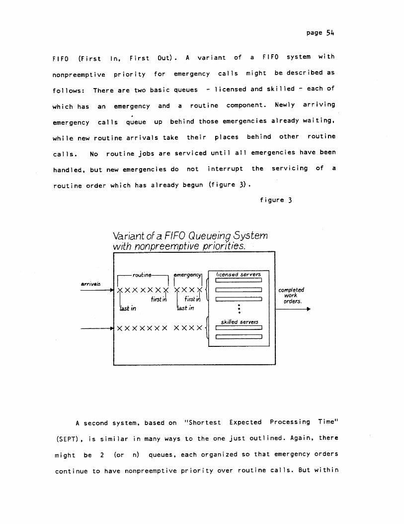
page 54
FIFO (First In, First Out). A variant of a FIFO system with
nonpreemptive priority for emergency calls might be described as
follows: There are two basic queues - licensed and skilled - each of
which has an emergency and a routine component. Newly arriving
emergency calls queue up behind those emergencies already waiting,
while new routine arrivals take their places behind other routine
calls. No routine jobs are serviced until all emergencies have been
handled, but new emergencies do not interrupt the servicing of a
routine order which has already begun (figure 3).
figure 3
Variant of a FIFO Queueing 5ystemwith nonpreemptive priorities.
arri. V4ls rouhne emergencyl licensed servers
XXX XXXXX X X X completedI I work
first m_ frst in - \ orders.Wkin Lfin
skilled server.sXXXXXXX XXXX
A second system, based on "Shortest Expected Processing Time"
(SEPT), is similar in many ways to the one just outlined. Again, there
might be 2 (or n) queues, each organized so that emergency orders
continue to have nonpreemptive priority over routine calls. But within

page 55
each emergency or routine sub-queue, those jobs are serviced first
which have the shortest expected processing (service) time. On any
day, this priority is assigned by the maintenance supervisor without
considering how long a given call may have already waited for service
(figure 4).
figure 4
A SEPT Queueing Systemwith nonpreemptive priorit le5.
routine emergency licensed servers
arrivals IIXXXXXXX XXX completed
workorders.
sept sept
skilled server.,XXXXXXX XXXX(
The FIFO and SEPT queueing systems can be compared with respect
to the total time tenants spend waiting in each system. Using monthly
data, a FIFO work order profile can be created by sorting calls at any
development according to craft (licensed or skilled) and then in
ascending order by arrival date. Note that "class" distinctions have
been ignored, since knowing when the emergency queue is empty involves
a more complex analysis, while the simplification used here does not
affect a comparison of the two policies.
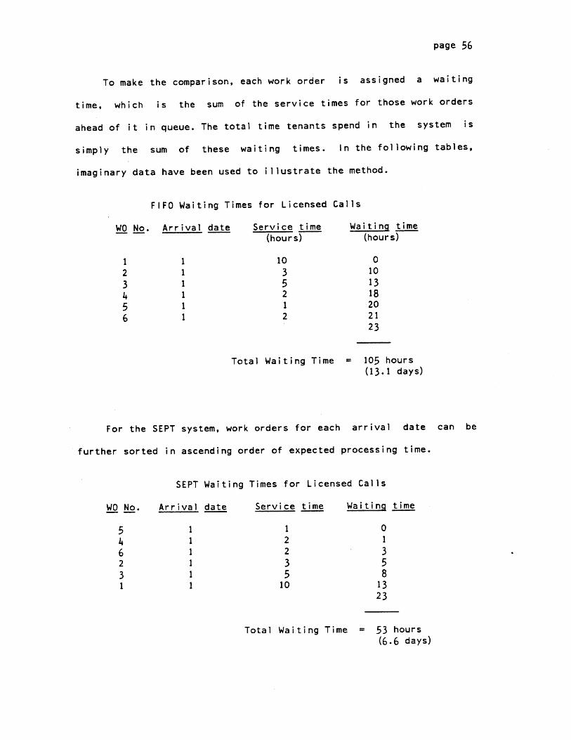
page 56
To make the comparison, each work order is assigned a waiting
time, which is the sum of the service times for those work orders
ahead of it in queue. The total time tenants spend in the system is
simply the sum of these waiting times. In the following tables,
imaginary data have been used to illustrate the method.
FIFO Waiting Times for Licensed Calls
WO No. Arrival date Service time Waiting time
(hours) (hours)
1 1 10 0
2 1 3 10
3 1 5 134 1 2 18
5 1 1 20
6 1 2 2123
Total Waiting Time 105 hours(13.1 days)
For the SEPT system, work orders for each arrival date can be
further sorted in ascending order of expected processing time.
SEPT Waiting Times for Licensed Calls
WO No. Arrival date Service time Waiting time
5 1 1 04 1 2 16 1 2 32 1 3 53 1 5 81 1 10 13
23
Total Waiting Time 53 hours
(6.6 days)

page 57
In practice, work orders are continuously arriving that have shorter
service times than some which may have just been serviced. Therefore,
the total waiting times calculated by this method are only
approximations of those we would actually witness. Nevertheless, a
comparison of these hypothetical policies provides reasonable evidence
that a queueing discipline based on Shortest Expected Processing Time
would be preferable to a simple FIFO system in terms of reducing the
total time tenants spend waiting for service. For equity reasons,
supervisors might want to put an upper limit on the time a work order
may be delayed due to its long expected processing time.
Other queueing disciplines could be evaluated in a similar
fashion by comparing the total waiting times implied by each policy.

page 58
APPENDIX I
Key to Tables in the Appendices
Appendix III
Tables 1,2 & Figure 1
- wos work orders. This is the number of work orders arriving perday.
- em emergency work orders- rou routine "- lic licensed " " "
- ski skilled " "
- emlic : emergency/licensed work orders arriving per day- emski : emergency/skilled " " " " " " "
- roulic : routine/licensed " " " " " "
- freq : frequencies or days on which n arrivals occurred- frac : the observed probability mass function, or the fraction of
days on which n arrivals occurred- Prn : the "expected" Poisson pmf. The observed mean arrival rate
used to calculate this distribution is the weighted mean ofthe orders arriving times the number of days on whichn arrive. The expected pmf is therefore a likely profile ofthe observed distribution if the observed is Poisson.
Table 3 :
- The calculations used for this test are pmfs given in table 7.
Table 4,5 & Figure 2
- Symbols are as in table 1 above. Also
- cumPrn : the cumulative expected pmf, or cumulative distributionfunction
- cumfrac : the cumulative observed pmf
- allKS : For all arrivals, this is the difference between cumPr_nand cumfrac, whose maximum value used as the D estimate inthe K-S test.
- eKS : same as allKS, but for emergency arrivals- rKS : " ' " "' "' routine "' "1- IKS : "o "t "' " licensed " "1
" " " " routine/skilled arrivals- rsKS : "

page 59
Tables 6,7 :
- wos : arrivals per day for all work orders- un20, un40, 60, 100 A set of 20, 40, 60, 100 uniformly
distributed random frequencies (days) onwhich n arrivals would occur.
- frac20, 40, 60, 100 Random uniform pmf based on un20, 40, ...100- uncdf20, 40, ...100 uniform cdfs based on frac20, ...100- poi_pmf20, 40, ...100 : Expected poisson pmfs were generated using
the mean arrival rate implied by theuniform istribution. Because they have thesame mean, we are testing how sensitive theregression and K-S tests are to the formsthe distributions take.
- poicdf20, ...100 : cdfs based on the poipmf20, ...100- D20, ...100 : Differences between the uncdf20, ...100 and
poicdf20, ...100. The maximum in this set is the Dstatistic used to test K-S sensitivity at samplesizes 20 to 100.
Appendix IV
Table 3 :
- hrs : service times in hours- emfrac observed pdf for emergency service times- rfrac " " " routine " " "
- rsfrac " " " " routine/skilled service times
- epdf : expected pdf for emergency service times- rpdf :" " " " routine " " "
- rspdf " " " " routine/skilled service times.
Table 4
- cepdf cumulative expected pdf for emergency service times- cefrac S " observed " " " " " "
- eks : differences between cepdf and cefrac

134817 BOSTON HOUSING AUTHORITY MAINTENANCE WORK ORDER
tLL W I I I I I0 E V U N I T
I I I 1 - I I IM M D D Y Y
DEV.NAME:
TENANT LAST NAME
REQUESTER - IF DIFFERENT FROM ABOVE
TEL NO.
TEL NO.
ADDRESS:
UNITFLOOR: SIZE: - BR.
(SEE REVERSE)
CLASS CRAFT
ERS?/L I I I I I ICLERK .D. INmALS
ASSIGNED:
DATE
STOCK NO. ITEM OUAN. UNIT 0 EXTENDED
TOTAL
CRAFTSMAN'S WORK DESCRIPTION
EMPLOYEE NO. NAME HRS. MINS. CODES
I I I I ISUPER ID. NO.
TIME
L IJ L J iEST. HRS. EST. LABOR EST. MATERIAL
TENANTS PERMISSION TO ENTER OR PERMISSION RECENED BY
DATE NOT HOME DATE NOT HOME DATE - VOID
(SEECAUSE: REVERSE)
TENANT ACCEPTANCE
COMPLETED BY
INSPECTED BY
M M D D
-I _jM M D D
M M D D
0c
0
~1
'I
0
0
r+0
0
c
0
C)
0
00%.#
.-
guz
-oQI
0 R
SUPERVISOR M M 0 D
BLUE: WORKMANIEDP WHITE: WORKMAN/SUPER YELLOW: TENANT PINC: W.O. CLERK
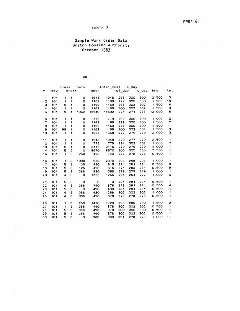
page 61
table 2
Sample Work Order DataBoston Housing Authority
October 1983
wo
class mats totalcost aday# dev craft labor ci day cday hrs tat
i 101 1 1 0 1948 1948 298 300 300 2.500 32 101 1 1 0 1169 1169 277 300 300 1.500 183 101 5 1 0 1169 1169 295 302 302 1.500 64 101 1 1 0 1169 1169 300 302 302 1.500 35 101 5 1 1962 12540 14502 271 274 278 12.000 6
6 101 1 1 0 779 779 299 300 300 1.000 27 101 1 1 0 1169 1169 299 300 300 1.500 28 101 1 1 0 1169 1169 286 300 300 1.500 119 101 99 1 0 1169 1169 300 302 302 1.500 3
10 101 1 1 0 1558 1558 277 279 279 2.000 3
11 101 1 1 0 1948 1948 279 277 279 2.500 112 101 1 1 0 779 779 294 302 302 1.000 713 101 5 1 0 3116 3116 279 279 279 4.000 114 101 5 2 0 8670 8670 305 305 305 7.500 115 101 1 3 250 490 740 278 278 278 0.500 1
16 101 1 3 1390 980 2370 298 298 298 1.000 117 101 5 3 125 490 615 271 281 281 0.500 918 101 5 3 125 490 615 271 283 291 0.500 919 101 5 3 388 980 1368 279 279 279 1.000 120 101 4 3 0 1256 1256 264 264 277 1.000 10
21 101 5 3 0 0 0 281 281 281 0.500 122 101 4 3 388 490 878 278 281 281 0.500 423 101 5 3 0 490 490 281 281 281 0.500 124 101 4 3 388 980 1368 302 302 302 1.000 125 101 4 3 388 490 878 278 278 278 0.500 1
26 101 1 3 250 1470 1720 298 286 299- 1.500 227 101 1 3 388 490 878 302 302 302 0.500 128 101 5 3 388 490 878 300 300 300 0.500 129 101 5 3 388 490 878 302 302 302 0.500 130 101 5 3 0 980 980 264 278 278 1.000 11

page 62
APPENDIX III -
1) Linear Regression as a Test of Probability Distributions
A simple regression test was devised to observe how closely the two
pmfs correspond by using one distribution as the independent
variable or predictor of the other. We assumed
the two sets of probabilities would match perfectly if the test
accounted for all
of the variation by fitting a line of slope-1, passing directly through
the origin.
Since we did not precisely know the extent of errors in the data,
the tests were run in several ways. First,
the observed pmf was used as the independent variable
to explain variations in the expected probabilities.
Pr{expected} = BO + B1 X Pr{observed} (1a)
This is a regression of the "expected on the observed" probabilities.
The relationship was then turned around to test how well the expected
Poisson pmf explained the observed variation.
Pr{observed} = BO + B1 X Pr{expected} (1b)
Although the fraction of total variation explained (r-square) is the
same in each case, the slopes (B1) and y-intercepts (BO) may differ.
We controlled the y-intercepts by eliminating the constant terms from
the equations and forcing the fitted lines to pass through the origin.
This second round of tests gave both different slopes and different

page 63
r-square values.
Pr{expected} = BI X Pr{observed}
Pr{observed} = BI X Pr{expected}
(2a)
(2b)
A comparison of the results from each of these four regressions was
initially used to indicate whether all arrivals to development 108
taken as a group could be approximated by a Poisson model. The test
results were
Pr {exp}
Pr {obs}
- 0.07
- 0.09
Pr {exp}
Pr {obs}
- 0.11 X Prfobs}
- 0.10 X Prfexp}
= 0.56 X Prfobs}
= 0.96 X Pr{exp}
r
r*-
r'-
r.r=
0.01
0.01
error
error
(1a)
(Ib)
(2a)
(2b)
Development
overall.(1)
108 arrivals certainly did not appear to be Poisson
We thought that arrivals for some classes and crafts
been more closely approximated by the Poisson model, however
summarizes regression results for each of the four equations
craft, and class/craft combination. The observed and
probabilities for each category are given in table
distributions are plotted in figures la through 1d.
All four series of regressions indicated that only e
licensed, emergency/licensed and emergency/skilled arriva
may have
. Table 1
by class,
expected
2. The
mergency,
Ils might
(1)In cases for which the correlation of the dependent and
independent variables is extremely small, the "rgop" program in the
Consistent System sometimes yields negative values for r-square when
the constant term is forced out of the model.

page 64
follow nearly Poisson patterns. All other classes and crafts appeared
to have non-Poisson arrivals, as indicated both by their low r-square
values and slopes nearer to zero than to one. But how reliable were
these results?
We then tested the regression test itself by generating a
distribution of random uniform probabilities and using regression to
compare them with a Poisson distribution. To calculate our Poisson
values, we used the mean arrival rate implied by the corresponding
uniform probabilities as our estimate of lambda. If the test showed no
correlation between the distributions (as we would expect), then we
would have had some evidence that the regression method used was
accurate enough for our purposes.
The results of these tests are given in table 3. They indicate
that regression is an inadequate tool for comparing noncumulative
probability distributions based on small samples. This explains why
our finely sliced categories appeared to be nearer to Poisson
distributions. For larger samples, the test distinguishes between
uniform and Poisson distributions, but not between the Poisson and the
normal. In addition, regressions using cumulative distributions were
shown to be extremely insensitive to any differences between
distributions.
Most important, however, the non-constant variances in the
distributions suggest the need for a weighted least squares approach
if regression models are to be used. Unfortunately, no time was
available to execute this test. On the basis of simple regression
tests, we could therefore neither accept nor reject the hypothesis
that observed arrivals are Poisson distributed.

Linear Regressions of Observed Arrivals on Expected Poisson Arrivals
Class/CraftCategory
Expected on Observed
2r BO B1i
Observed on Expected
2r B0 B1i
Exp. on Obs.
2r B1i
Obs. on Exp.
2r B1
All workorders
Emergency
Routine
Licensed
Skilled
Emlic
Emski
Roulic
Rouski
.01 .07*
.57
.00
.02
.08
.54 .02
.10 .04
.11
.63
.03
.71
.40
.90 -. 03 1.07
.53
.07
.10
*.02 .83
.08 .50
*.07 .34
.01 .09 -. 10
.57
.00
.54
.10
.90
.53
*.03
.08
.04
.08
.91
.04
.76
.24
.04 .84
*.06 .64
.07 .14 .15
.10 .08 .29
error .56
.54 .74
error .69
.53 .81
error .96 0
.52 1.13
error .75
.44 1.03
.03 .71 error .92
.89
.52
.96
.92
error .93
error .83
.85 1.01
.36 .94
error .90
error .85
* - insigcnificant WO coefficient, indicating the fittedl line may nass through the origin.
I-
Di
CT'
0
a a Ca
om
0
oo -< --
0Di'
0
r+
0-ow
0
"0:3
In DitoID
0*'I.,,

table 2 Observed & Expected Poisson Probability Mass Functionsby Class & Craft, Development 108
frac Pr_n
0.050 0.0030.150 0.0210.050 0.0390.100 0.0620.050 0.1070. 100 0.1190.100 0.1100.050 0.0940.050 0.0550.100 0.0380.150 0.0250.050 0.015
f reqem frac Pr n.
1 32 33 34 66 1
7 18 1
10 112 1
0.150 0.0610.150 0.1290.150 0.1830.300 0.1940.050 0.117
0.050 0.0710.050 0.0380.050 0.0080.050 0.001
t reqrou frac Pr_n
2 1 0.050 0.0293 5 0.250 0.0634 1 0.050 0.1055 2 0.100 0.1406 2 0.100 0.1557 1 0.050 0.1488 1 0.050 0.1239 2 0.100 0.09110 1 0.050 0.06011 2 0.100 0.036
12 1 0.050 0.02013 1 0.050 0.010
lic fracf req
1 3 0.153 4 0.204 5 0.255 2 0.106 1 0.05
7 18 29 10 1
f reqski f rac Pr_nPr_n
0 0.0650 0.1880 0.1950 0.1620 0.112
1 1 0.0502 3 0.1504 2 0.1005 1 0.0506 2 0.100
7 3 0.1508 3 0.150
11 3 0.15012 1 0.05013 1 0.050
0.050 0.0660.100 0.0340.050 0.0160.050 0.016
eml icfreq f rac Pr_n
1 7 0.350 0.3292 4 0.200 0.2553 3 0.150 0.1327 1 0.050 0.0010 5 0.-250 0.212
roul icfreqfrac Pr_n
1 3 0.150 0.1992 4 0.200 0.2543 4 0.200 0.2164 2 0.100 0.1385 4 0.200 0.0700 3 0.150 0.078
emsk if req f rac Pr_n
1 5 0.250 0.1872 4 0.200 0.2483 4 0.200 0. 2194 1 0.050 0.1455, 3 0.150 0.0779 1 0.050 0.0010 2 0.100 0.071
rousk ifreqfrac Pr_n
1 3 0.150 0.0562 2 0. 100 0.1223 5 0.250 0. 1774 2 0.100 0.1935 1 0.050 0. 1686 2 0.100 0. 1217 2 0.100 0.0758 2 0.100 0.041
10 1 0.050 0.009
Column 1 = number of arrivalsColumn 2 = freqencies ,(days)Column 3 = "frac" = observed probabilitiesColumn 4 = "Pr n" = exTected Poisson omf
f req
page 66
wos
3567911121315161718
0.0080.0270.1010.1370. 154
0.1480. 1250.0390.0220.011
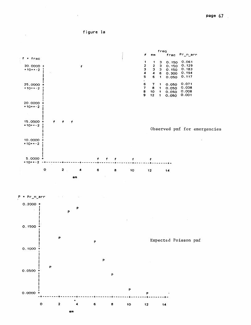
page 67
figure la
f req# em frac Pr_narr
2345
12346
3336i
6 7 17 818 10 19 12 1
0. 1500.1500.1500.3000.050
0.0500.0500.0500.050
0.0610.1290. 1830. 1940. 117
0.0710.0380.0080.001
15.0000 +*10*-2
10.0000 +*10**-2
5.0000 +*10**-2 -+-
f f f
Observed pmf for emergencies
f f f f f------------- + ----------- --------------------- +-----------
0 2 4 6 8 10 12 14
em
P - Pr_n_arr
0.2000 +
I-0. 1500 +
0. 1000 +
0.0500 +
0.0000 +
P
P
P
Expected Poisson pmfP
P
P
P
PP
--2- 46-8-1-1+---------------------------------------------
0 2 4 6 a 10 12 14
em
f = f rac
30.0000 +*10**-2
25.0000 +*10**-2
f
20.0000*10**-2
+
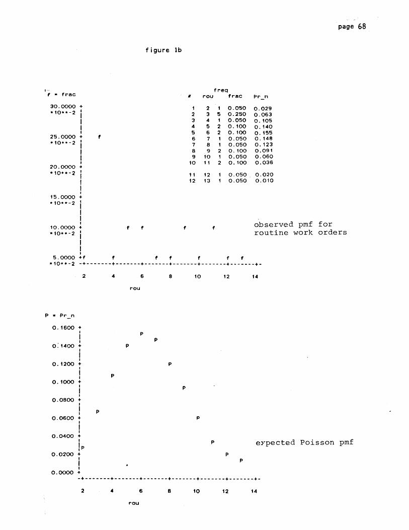
f
page 68
figure lb
f = frac
30.0000 +*10**-2
25.0000 +*10**-2
20.0000 +*10**-2
15.0000 +*10**-2
10.0000 +*10**-2
5.0000 +f*10**-2 -+-
f req# rou frac Pr_n
123456789
10
23456789
1011
i5222
1
2
2
0.0500.2500.0500.1000.1000.0500.0500.1000.0500. 100
0.0290.0630.1050.1400. 1550. 1480.1230.0910.0600.036
11 12 1 0.050. 0.02012 13 1 0.050 0.010
f f
f f---- +--------------
f
f
f observed pmf forroutine work orders
f f f----------------------
2 4 6 8 10 12 14
rou
P = Pr n
P
P
P
P
P
P
erpected Poisson pmf
P
- 4 62-----.----------- 1----------------------------4
2 4 6 a 10 12 14
P
PP
0. 1600 +
0.1400 +
0.1200 +
0.1000 +
0.0800 +
0.0600 +
0.0400 +
0.0200 +
0.0000 +
P
rou
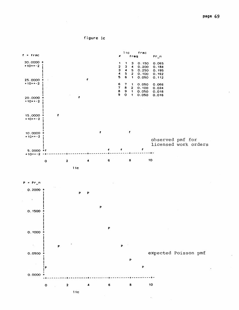
page 69
figure ic
f = frac
30.0000 +*10**-2
25.0000 +*10**-2
20.0000 +*10**-2
15.0000 +*10.*-2
10.0000 +*10+*-2
5.0000 +f*10**-2 -+-
0
f
ic frac# freq
1 1 3 0.1502 3 4 0.2003 4 5 0.2504 5 2 0.1005 6 1 0.050
6 7 1 0.0507 8 2 0.1008 9 1 0.0509 0 1 0.050
Pr-n
0.0650.1880. 1950. 1620.112
0.0660.0340.0160.016
f
f f
observed pmf forlicensed work orders
f f f------------+--------------+----------------------------
2 4 6 8 10
l ic
P = Pr_n
0.2000 +
0. 1500 +I
0. 1000 +
0.0500 +
.P
0.0000 +
0
P P
P
P
P P
expected Poisson pmf
P
P
-+-------- ----- +-----------+---------------------------
2 4 6 8 10
lic

page 70,
figure Id
f req# ski frac Pr_n
1 1 1 0.0502 2 3 0.150
f 3 4 2 .1004 5 1 0.0505 6 2 0.100
0.1500. 1500.1500.0500.050
6 7 37 8 38 11 39 12 1
10 13 1
0.0080.0270.1010. 1370. 154
0.1480. 1250.0390.0220.011
observed pmf forskilled work orders
f f
4 6 8 10 12 14
ski
PP
P
P
P
P
P+ P
P+
expected Poisson pmfP
4 6 8 10 12 14
+
+
+
f f
f = frac
16.0000*10**-2
14.0000*10**-2
12.0000*10**-2
10.0000* 10** -2
8.0000*10**-2
6.0000* 10**-2
4 .0000*10**-2
+
++
f
0 2
P = Pr n
0. 1600 +
0..1400 +
0. 1200 +
0.1000 +
0.0800 +
0.0600 +
0.0400 +
0.0200
0.0000
0 2
ski
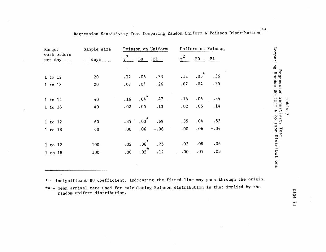
R s *Regression Sensitivity Test Comparing Random Uniform & Poisson Distributions
Range:work ordersper day
1 to 12
1 to 18
1 to 12
1 to 18
1 to 12
1 to 18
1 to 12
1 to 18
Sample size
days
20
20
40
40
60
60
100
100
Poisson on Uniform
2r BO B1
.12 .06 .33
.07 .04
.16 .04
.02 .05
*.35 .03
.26
.47
.13
.69
.00 .06 -. 06
*.02 .06
*.00 .05
.25
.12
Uniform on Poisson
2r BO B1
*.12 .05 .36
.07 .04 .25
.16 .06 .34
.02 .05 .14
.35 .04 .52
.00 .06 -.04
.02 .08 .06
.00 .05 .03
* - insignificant BO coefficient, indicating the fitted line may pass through the origin.
** - mean arrival rate used for calculating Poisson distribution is that implied by the
random uniform distribution.
C)0
Xh M
0~0
0
0-I
o" r+
r+
=1
Cr
0
-u

TABLE 4 Appendix III Kolmogorov-Smirnov Goodness of Fit Test for Arrivals, by Class & Craft,Developmvent 108
Class/CraftCategory
All workorders
Emergency
Routine
Licensed
Skilled
Emlic
Emski
Roulic
Rouski
D statistic
.213
.184
.199
.086
.164
.038
.100
.156
.145
n (sample size)
20
20
20
20
20
20
20
20
20
Critical Values
a=.20 a=.05
.231
.231
.231
.231
.231
.231
.231
.231
.231
.294
.294
.294
.294
.294
.294
.294
.294
.294
Decision
accept
accept
accept
accept
accept
accept
accept
accept
accept
Ho: observed=PoissonHI: observedtPoisson
0
0(00in0
0. C- 0(/1
(<<
CD 0 M~-- 0
oo
0.- 0UCO -
r+ '
rtlu
CD
--I
r+
0~1
"-a

page 73
table 5
oumfrac2cumPr n
0.0050.0350.0750.1370.330
0.5670.6780.7720.9020.940
0.9650.981
0.0500.2000.2500.3500.400
0.5000.6000.6500.7000.800
0.9501.000
Kolmogorov-Smirnov Test Calculationsby class & craft
al IKS
-0.045-0.165-0.175-0.213-0.070
0.0670.0780.1220.2020.140
0.015-0.019
development 108
freqem cumfrac
1 3 0.1502 3 0.3003 3 0.4504 6 0.7506 1 0.800
7 1 0.8508 1 0.900
10 1 0.95012 1 ' 1.000
cumPr
0.0610.1890.3720.5660.847
0.9180.9560.9810.985
eKS
-0.089-0.111-0.078-0.1840.047
0.0680.0560.031
-0.015
f reqrou cumfrac
2 13 54 15 26 2
7891011
212
curnPr
0.050 0.0370.300 0.1010.350 0.2060.450 0.3460.550 0.502
0.600 0.6490.650 0.7720.750 0.8630.800 0.9230.900 0.960
12 1 0.950 0.98013 1 1.000 0.990
lic cumfracfreq cumPr 1KS
f reqski cumfrac
1 3 0.150 0.1313 4 0.350 0.3514 5 0.600 0.5465 2 0.700 0.7086 1 0.750 0.820
7 1 0.800 0.8868 2 0.900 0.9209 1 0.950 0.9360 1 1.000 0.952
-0.0190.001
-0.0540.0080.070
0.0860.020
-0.014-0.048
1 1 0.050 0.0092 3 0.200 0.0364 2 0.300 0.1975 1 0.350 0.3346 2 0.450 0.488
7 3 0.600 0.6368 3 0.750 0.761
11 3 0.900 0.95712 1 0.950 0.97913 1 1.000 0.990
emlic cumfracfreq cumPr elKS
emski cumfracfreq cumPr esKS ,
1 7 0.350 0.329 -0.0212 4 0.550 0.584 0.0343 3 0.700 0.716 0.0167 1 0.750 0.788 0.0380 5 1.000 1.000 -0.000
1 5 0.250 0.187 -0.0632 4 0.450 0.435 -0.0153 4 0.650 0.654 0.0044 1 0.700 0.800 0.1005 3 0.850 0.877 0.027
9 1 0.900 0.929 0.0290 2 1.000 1.000 -0.000
cumfracroulic
freq cumPr rIKSrouski cumfrac
freq cumPr rsKS
1 3 0.150 0.199 0.0492 4 0.350 0.453 0.1033 4 0.550 0.669 0.1194 2 0.650 0.806 0.1565 4 0.850 0.876 0.026
0 3 1.000 0.955 -0.045
1 3 0.150 0.056 -0.0942 2 0.250 0.178 -0.0723 5 0.500 0.355 -0.1454 2 0.600 0.548 -0.0525 1 0.650 0.715 0.065
6 2 0.750 0.837 0.0877 2 0.850 0.912 0.0628 2 0.950 0.953 0.00310 1 1.000 0.982 -0.018
cumPrsKS
-0.041-0.164-0.103-0.0160.038
0.0360.0110.0570.029
-0.010
rKS
-0.013-0. 199-0.144-0.104-0.048
0.0490.1220.1130. 1230.060
0.030-0.010

page 74figure 2
c = cumfrac
C1.0000
0.8000
C
C
CC
0.6000 +
0.4000 +
0.2000 +
0.0000
0
C
C
CC
CC
C observed cdf, allwork orders
5 10 15 20
wos
c = cumPr_n
1.0000 +
0.8000 +
0.6000 +
0.4000 +
0.2000 +
0.0000 +
0
CC C
C
C
C
C
C
Cexpected Poisson cdfc
CC
1o 15 20
wos

Kolmogorov-Smirnov Sensitivity Test Comparing Random Uniform and Poisson Distributions *
Pange:work ordersner day
1 to 12
1 to 18
1 to 12
I to 18
1 to 12
1 to 18
1 to 12
1 to 18
Sample size
n
20
20
40
40
60
60
100
100
D statistic
D
.147
.236
.166
.176
.104
.227
.152
.199
Critical Values
a = .20 a = .05
.231
.231
.169
.169
.138
.138
.107
.107
.294
.294
.215
.215
.176
.176
.136
.136
Decision
accept Ho
reject at
accept at
accept Ho
reject at
accept at
accept Ho
reject Ho
reject Ho
reject Ho
.20
.05
.20
.05
Ho: uniform = Poisson(test insensitive todifferences at this n)
Hi: test sensitive atleast to differencesbetween uniform & Poissonat this n
0
0I0
0-,
930VV <0w 1
r+ M
EnC r
0 0-D 1r
* - mean arrival rate used for calculating Poisson distribution is that implied by the
random uniform distribution.
w
a'
-UDi£0CD
'-TI
Table 6
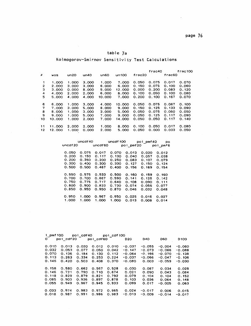
page 76
table 7a
Kolmogorov-Smirnov Sensitivity Test Calculations
wos un20 un40 un60 unIO frac20
1.0002.0003.0004.0005.000
6.0007.0008.0009.000
10.000
1.0003.0000.0002.0004.000
1.0003.0001.0001.0001.000
3.0003.0008.0002.0004.000
3.0005.0003.0005.0002.000
1.0006.0005.0006.000
10.000
4.0008.0003.0007.0007.000
7.0006.000
12.0008.0007.000
10.0009.0005.0009.000
14.000
0.0500.1500.0000.1000.200
0.0500.1500.0500.0500.050
frac40
0.0750.0750.2000.0500.100
0.0750.1250.0750.1250.050
frac 100frac60
0.0170.1000.0830.1000.167
0.0670.1330.0500.1170.117
0.0700.0600.1200.0800.070
0.1000.0900.0500.0900.140
11 11.000 2.000 2.000 1.000 8.000 0.100 0.050 0.017 0.08012 12.000 1.000 0.000 2.000 5.000 0.050 0.000 0.033 0.050
uncdf 20
0.0500.2000.2000.3000.500
0.5500.7000.7500.8000.850
Uncdf 40
0.0750.1500.3500.4000.500
0.5750.7000.7750.9000.950
uncdf6C
0.0170.1170.2000.3000.467
0.5330.6670.7170.8330.950
uncdfiOO poi_pmf4O POpoipmf2O poi_pmf6
0.0700.1300.2500.3300.400
0.5000.5900.6400.7300.870
0.0130.0400.0830.1270.156
0.1600.1410.1080.0740.046
0.0200.0570.1070.1500.169
0.1590.1280.0900.0560.032
0.0120.0380.0790.1240.154
0.1600. '420.1110.0770.048
0.950 1.000 0.967 0.950 0.025 0.016 0.0271.000 1.000 1.000 1.000 0.013 0.008 0.014
i_pmf 100 poi_cdf40 poi-cdfIOC0 poicdf2O poilcdf6O
0.0130.0530.1360.2630.420
0.5800.7210.8290.9030.949
0.0200.0770.1840.3340.503
0.6620.7900.8790.9360.967
0.0120.0500.1300.2530.408
0.5670.7100.8210.8970.945
0.0100.0420.1120.2240.370
0.5280.6740.7920.8780.933
D20 D40 D60 DiO0
-0.037-0.147-0.064-0.037-0.080
0.0300.0210.0790.1030.099
-0.055-0.073-0.166-0.0660.003
0.0870.0900.1040.0360.017
-0.004-0.066-0.070-0.047-0.059
0.0340.0430.1040.064
-0.005
-0.060-0.088-0.138-0.106-0.030
0.0280.0840.1520. 1480.063
0.033 0.974 0.983 0.972 0.965 0.024 -0.017 0.006 0.0150.018 0.987 0.991 0.986 0.983 -0.013 -0.009 -0.014 -0.017
12345
678910
0.0100.0320.0700.1130.146
0.1580.1460.1180.0850.055

page 77
table 7bKolmogorov-Smirnov Sensitivity Test Calculations
# wos2 un20 un40 un6O uniO frac20
1.0002.0003.0004.0005.000
6.0007.0008.0009.000
10.000
11.00012.00013.00014.00015.000
16.00017.00018.000
1.0001.0001.0003.0000.000
0.0001.0001.0002.0003.000
2.0000.0001.0002.0001.000
1.000.0.0000.000
0.0003.0003.0001.0002.000
3.0002.0000.0000.0002.000
6.0006.0001.0003.0001.000
12345
678910
1112131415
161718
uncuncdf20
0.0500.1000.1500.3000.300
0.3000.3500.4000.5000.650
0.7500.7500.8000.9000.950
pmf 100
0.0010.0050.0160.0350.063
0.0940.1190. 1330.1320.117
0.0950.0710.0490.0310.018
0.0100.0050.003
1.0001.0001.000
poi_cdf20
0.0010.0070.0250.0640.132
0.2300.3540.4890.6200.735
0.8260.8930.9380.9660.982
0.9910.9960.998
0.0.0.0.0.
0.0.0.0.0.
0.0.0.0.0.
0.0.1 .
3.0001.0005.0006.0003.000
0.0001.0006.0002.0002.000
7.0002.0002.0004.0006.000
.000 4.000
.000 6.000
.000 0.000df40
uncdf60
000 0.050075 0.067150 0.150175 0.250225 0.300
300 0.300350 0.317350 0.417350 0.450400 0.483
550 0.600700 0.633725 0.667800 0.733825 0.833
950 0.900975 1.00000 1.000
poi_cdf60
1.00010.00010.0004.0007.000
6.0006.0005.0007.0002.000
8.0005.0007.0007.0002.000
4.0004.0005.000
incdf 100
0.0100.1100.2100.2500.320
0.3800.4400.4900.5600.580
0.6600.7100.7800.8500.870
0.910 C0.950 C1.000 C
D2poi_cdf40 poicdfiO
0.0000.0030.0100.0270.063
0.1240.2110.3220.4450.570
0.6850.7820.8570.9110.948
0.9710.9840.992
0.0010.0030.0110.0320.073
0.1400.2340.3500.4770.602
0.7140.8060.8750.9240.956
0.9760.9870.994
0.0010.0070.0220.0580.121
0.2140.3330.4660.5980.715
0.8110.8810.9300.9610.979
0.9900.9950.998
-0.049-0.093-0.125-0.236-0.168
-0.0700.0040.0890.1200.085
0.0760.1430.1380.0660.032
-0.009-0.004-0.002
0.0500.0500.0500.1500.000
0.0000.0500.0500.1000.150
0.1000.0000.0500.1000.050
0.0500.0000.000
frac40
0.0000.0750.0750.0250.050
0.0750.0500.0000.0000.050
0.1500.1500.0250.0750.025
0.1250.0250.025
fraclOOfrac60
0.050 0.0100.017 0.1000.083 0.1000.100 0.0400.050 0.070
0.000 0.0600.017 0.0600.100 0.0500.033 0.0700.033 0.020
0.117 0.0800.033 0.0500.033 0.0700.067 0.0700.100 0.020
0.0670. 1000.000
0.0400.0400.050
pmf20 pmf40 pmf60
).001).006).018).039).068
0.0990.123O.1350.131).115
0.0910.0670.0450.0280.016
.009
.005
.0020
0.0000.0020.0070.0180.036
0.0610.0870.1100.1240.125
0.1150.0970.0750.0540.036
0.0230.0140.008
0.0010.0030.0080.0210.041
0.0670.0940.1160. 1270.125
0.1120.0920.0700.0490.032
0.0200.0110.006
D40 D60 D100
0.000-0.072-0.140-0.148-0.162
-0.176-0.139-0.0280.0950.170
0.1350.0820.1320.1110.123
0.0210.009
-0.008
-0.049-0.064-0. 139-0.218-0.227
-0.160-0.083-0.0670.0270.118
0.1140.1720.2080.1910.123
0.076-0.013-0.006
-0.009-0.103-0.188-0.192-0.199
-0.166-0.107-0.0240.0380.135
0.1510.1710.1500.1110.109
0.0800.045
-0.002
511
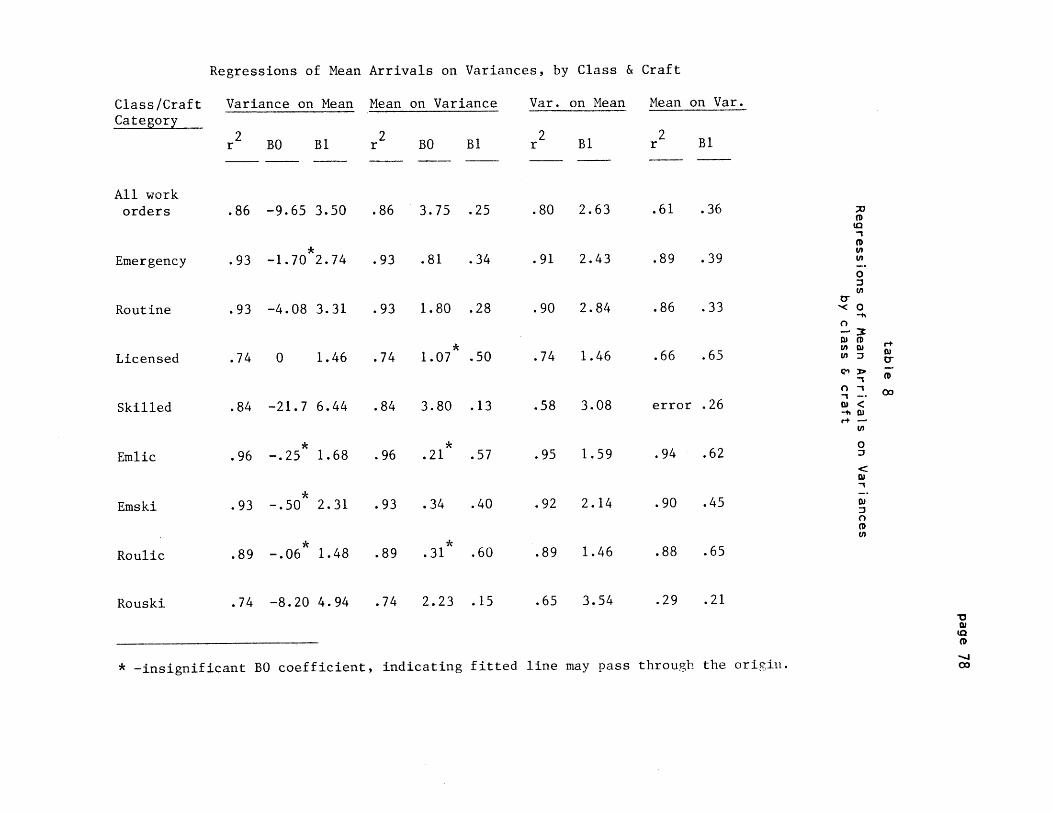
Regressions of Mean Arrivals on Variances, by Class & Craft
Class/CraftCategory
All workorders
Emergency
Routine
Licensed
Skilled
Emlic
Emski
Roulic
Rouski
Variance on Mean
2r BO B1
.86 -9.65 3.50
.93 -1.70 2.74
.93 -4.08 3.31
Mean on Variance
r BO BI
.86 3.75 .25
.93 .81 .34
.93 1.80 .28
.74 0 1.46 .74 1.07
.84 -21.7 6.44
.96 -. 25 1.68
*.93 -. 50 2.31
*.89 -. 06 1.48
.74 -8.20 4.94
.50
.84 3.80 .13
.96 .21 .57
.93 .34 .40
*.89 .31 .60
.74 2.23 .15
Var. on Mean
r2 B1
.80 2.63
.91 2.43
.90 2.84
.74 1.46
.58 3.08
.95 1.59
.92 2.14
.89 1.46
.65 3.54
Mean on Var.
r2 BI
.61 .36
.89 .39
.86 .33
.66 .65
error .26
.94 .62
.90 .45
.88 .65
.29 .21
-o01toCD
00* -insignificant BO coefficient, indicating fitted line may pass through the origin.
to
-I
0
0
t
D<
0
Di
(n
r+
00
page 79
APPENDIX IV
1) Use of Regression to Test Exponential Service Times
Using linear regression, the exponential distribution was
compared with observed probabilities representing the fraction of
actual service times that have a particular length. Regressions were
run on the noncumulative probabilities just as they were for arrivals,
using the same series of simple regression equations. Table 2
presents the results of these tests, and table 3 gives the actual
distributions. Slopes given by the "observed on expected" regressions
are in all cases fairly close to one, but an analysis of variation in
the other direction (expected on observed) suggests that service times
are non-Poisson. With the conservative decision rule that Poisson
processes should have r-squares over 50 and slopes between 60 and 140
in each of the four regressions, we conclude that service times are
not Poisson. In no cases, however, do the observed service time
distributions differ wildly from the Poisson model. These
distributions are also more homogenous across classes and crafts than
are the arrival rates.
Once more, however, the problem of inhomogenous variance makes
the results of these regression tests unreliable. A weighted least
squares approach should be used to account for non-constant variances.
Following is a collection of data, calculations and scatter plots
used in the service time analyses.
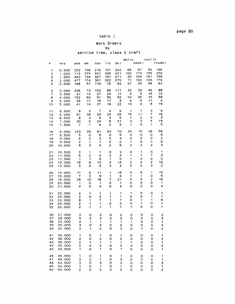
table 1
Work Ordersby
service time, class & craft
emlic roulic# hrs wos em rou lic ski emski rouski
1 0.500 352 138 210 127 222 68 67 59 1582 1.000 719 275 441 295 421 100 174 195 2503 1.500 463 134 327 191 271 30 104 161 1684 2.000 477 174 301 202 275 71 103 129 1745 2.500 168 57 110 76 92 27 30 48 63
6 3.000 206 73 133 88 117 42 30 46 887 3.500 41 14 27 24 17 9 5 15 128 4.000 152 60 91 59 92 24 35 35 589 4.500 26 11 15 17 9 6 5 i 410 5.000 41 14 27 18 22 10 4 8 19
11 5.500 9 2 7 4 5 1 1 3 412 6.000 51 26 24 23 28 15 11 7 1813 6.500 9 3 6 4 5 1 2 3 314 7.000 30 6 24 8 21 3 3 5 1915 7.500 7 1 6 2 5 1 0 1 5
16 8.000 123 39 81 53 70 24 15 28 5617 8.500 5 0 5 0 5 0 0 0 518 9.000 4 2 2 0 4 0 2 0 219 9.500 2 1 1 2 0 1 0 1 020 10.000 8 3 5 2 6 0 3 2 3
21 10.500 2 1 1 0 2 0 1 0 122 11.000 6 2 4 2 4 1 1 1 323 11.500 1 1 0 1 0 1 0 0 024 12.000 18 6 12 4 14 2 4 2 1025 13.000 5 0 5 3 2 0 0 3 2
26 14.000 17 6 11 1 16 0 6 1 1027 15.000 7 2 5 1 6 1 1 0 528 16.000 28 10 18 7 21 5 5 2 1629 20.000 1 0 1 0 1 0 0 0 130 21.000 4 0 4 0 4 0 0 0 4
31 22.000 2 1 1 1 1 1 0 0 132 23.000 2 0 2 1 1 0 0 1 133 24.000 8 1 7 1 7 0 1 1 634 25.000 2 1 1 0 2 0 1 0 135 2G.000 2 1 1 1 1 1 0 0 1
36 27.000 2 0 2 0 2 0 0 0 237 28.000 5 2 3 0 5 0 2 0 338 29.000 2 1 1 1 1 1 0 0 139 30.000 4 0 4 0 4 0 0 0 440 32.000 3 1 2 0 3 0 1 0 2
41 34.000 1 0 1 0 1 0 0 0 142 38.000 2 0 2 0 2 0 0 0 243 39.000 2 1 1 1 1 1 0 0 144 40.000 2 0 2 0 2 0 0 0 245 43.000 1 0 1 0 1 0 0 0 1
46 45.000 1 0 I 0 1 0 0 0 I47 48.000 3 2 1 0 3 0 2 0 148 52.000 3 0 3 0 3 0 0 0 349 54.000 1 0 1 0 1 0 0 0 150 64.000 2 0 2 0 2 0 0 0 2
page 80

Linear Regressions of Observed Service Times on Expected
Class/Craft Expected on
2r
All workorders
Emergency
Routine
Observed
BO BI
.63 .02 .51
.57 .02
.65 .02
Licensed .44 .02
.59
.32
.64
.45
.56
.48
.52
.41
.02 .43
.03
.02
.02
.02
.31
.49
.41
.40
Observed on Expected
2r BO B1
.63 0 1.24
.57 0 1.19
.65 0 1.26
.44 0 1.07
*.59 -.01 1.36
.32 0 1.03
.64 0 1.30
.45 0 1.08
.56 -. 01 1.39
Exp. on Obs.
2r B1i
.49 .64
.43 .62
.54 .65
.25 .56
.39 .57
error .48
.51 .61
.28 .55
.32 .55
Category
indicating fitted line may pass through the origin.
Obs. on Exp.
2r B1
.62 1.17
.57 1.15
.65 1.19
.44 1.09
.58 1.23
.32 1.07
.63 1.21
.45 1.10
.55 1.24
Skilled
Emlic
Emski
Roulic
Rouski
M0)
MU:)
-
-o 0
mo-sm
0
C<
rex
< 0C0)
00--ft
OC+
n
X
0
M..-
(n,CD
(n"U
r-
aa-
CD
* -insignificant BO coefficient,

page 82
table 3
Observed & Expected Service Time Probability Density Functionsby class & craftdevelopment 108
hrs emfrac epdf
0.5001.0001.5002.0002.5003.0003.5004.0004.5005.0005.5006.0006.5007.0008.0009.000
10.00011.00012.00016.00022.00024.00030.000
0.0800.2500.1100. 1300.0300.1400.0000.0700.0100.0200.0100.0400.0000.0000.0700.0100.0000.0000.0100.0200.0000.0000.000
0.1400.1190.1010.0850.0720.0610.0520.0440.0370.0320.0270.0230.0190.0160.0230.0170.0120.0090.0060.0020.0000.0000.000
rfrac rpdf ifrac 1pdf sfrac spdf
0.0850.2230.1490.1760.0320.0960.0050.0480.0160.0370.0000.0320.0110.0110.0480.0000.0050.0050.0000.0000.0050.0110.005
0.1400.1180.1000.0850.0720.0610.0520.0440.0370.0320.0270.0230.0190.0160.0240.0170.0120.0090.0060.0020.0000.0000.000
0.0610.1400.1050.2630.0440.1750.0090.0610.0180.0260.0000.0530.0090.0000.0180.0000.0000.0000.0000.0090.0000.0090.000
0.1480. 1240.1040.0870.0730.0610.0510.0430.0360.0300.0250.0210.0180.0150.0210.0150.0100.0070.0050.0010.0000.0000.000
0.0980.2990.1610.0980.0230.0690.0000.0460.0110.0290.0060.0230.0060.0060.0800.0060.0060.0060.0060.0060.0060.0060.006
0.1380.1170.1000.0850.0720.0610.0520.0440.0380.0320.0270.0230.0200.0170.0240.0180.0130.0090.0070.0020.0000.0000.000
hrs elfrac elpdf esfrac espdf rifrac rlpdf rsfrac rspdf
0.5001.0001.5002.0002.5003.0003.5004.0004.5005.0005.5006.0006.5007.0008.0009.000
10.00011.00012.00016.00022.00024.00030.000
0.0270.1890.0810.1620.0270.2430.0000.0810.0000.0270.0000.0810.0000.0000.0540.0000.0000.0000.0000.0270.0000.0000.000
0.1320.1130.0970.0830.0710.0610.0520.0450.0390.0330.0280.0240.0210.0180.0260.0190.0140.0100.0080.0020.0000.0000.000
0.1130.2900. 1290.1130.0320.0810.0000.0480.0160.0160.0160.0160.0000.0000.0810.0160.0000.0000.0160.0160.0000.0000.000
0. 1470.1230.1030.0870.0730.0610.0510.0430.0360.0300.0260.0210.0180.0150.0210.0150.0110.0080.0050.0010.0000.0000.000
0.0790. 1180.1180.3030.0530.1450.0130.0530.0260.0260.0000.0390.0130.0000.0000.0000.0000.0000.0000.0000.0000.0130.000
0.1560.1290.1070.0890.0730.0610.0500.0420.0350.0290.0240.0200.0160.0130.0180.0130.0090.0060.0040.0010.0000.0000.000
0.0920.2940.1740.0920.0180.0640.0000.0460.0090.0370.0000.0280.0090.0090.0830.0000.0090.0090.0000.0000.0090.0090.009
0.1310.1130.0970.0830.0710.0610.0520.0450.0390.0330.0280.0240.0210.0180.0260.0190.0140.0110.0080.0020.0000.0000.000
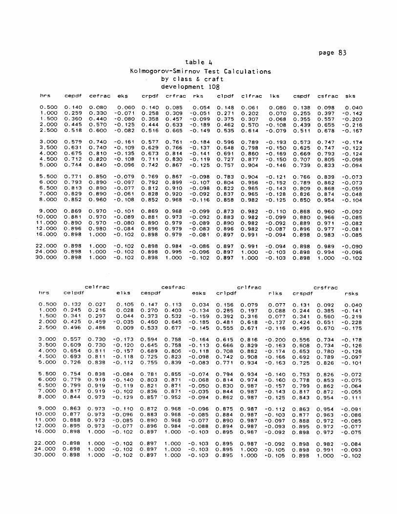
page 83table 4
Kolmogorov-Smirnov Test Calculationsby class & craftdevelopment 108
hrs cepdf cefrac eks crpdf crfrac rks clpdf clfrac lks cspdf csfrac sks
0.140 0.080 0.060 0.140 0.0850.259 0.330 -0.071 0.258 0.3090.360 0.440 -0.080 0.358 0.4570.445 0.570 -0.125 0.444 0.6330.518 0.600 -0.082 0.516 0.665
0.579 0.740 -0.161 0.577 0.7610.631 0.740 -0.109 0.629 0.7660.675 0.810 -0.135 0.673 0.8140.712 0.820 -0.108 0.711 0.8300.744 0.840 -0.096 0.742 0.867
0.771 0.850 -0.079 0.769 0.8670.793 0.890 -0.097 0.792 O.8990.813 0.890 -0.077 0.812 0.9100.829 0.890 -0.061 0.828 0.9200.852 0.960 -0.108 0.852 0.968
0.869 0.970 -0.101 0.869 0.9680.881 0.970 -0.089 0.881 0.9730.890 0.970 -0.080 0.890 0.9790.896 0.980. -0.084 0.896 0.9790.898 1.000 -0.102 0.898 0.979
0.898 1.000 -0.102 0.898 0.9840.898 1.000 -0.102 0.898 0.9950.898 1.000 -0.102 0.898 1.000
0.054 0.148 0.061-0.051 0.271 0.202-0.099 0.375 0.307-0.189 0.462 0.570-0.149 0.535 0.614
-0.184 0.596 0.789-0.137 0.648 0.798-0.141 0.691 0.860-0.119 0.727 0.877-0.125 0.757 0.904
-0.098 0.783 0.904-0.107 0.804 0.956-0.098 0.822 0.965-0.092 0.837 0.965-0.116 0.858 0.982
-0.099 0.873 0.982-0.092 0.883 0.982-0.089 0.890 0.982-0.083 0.896 0.982-0.081 0.897 0.991
-0.086 0.897 0.991-0.096 0.897 1.000-0.102 0.897 1.000
0.0860.0700.068
-0.108-0.079
-0.193-0.150-0.169-0.150-0.146
-0.121-0.152-0. 143-0.128-0.125
-0.110-0.099-0.092-0.087-0.094
-0.094-0.103-0.103
0.138 0.0980.255 0.3970.355 0.5570.439 0.6550.511 0.678
0.573 0.7470.625 0.7470.669 0.7930.707 0.8050.739 0.833
0.766 0.8390.789 0.8620.809 0.8680.826 0.8740.850 0.954
0.868 0.9600.880 0.9660.889 0.9710.896 0.9770.898 0.983
0.898 0.9890.898 0.9940.898 1.000
cel frachrs celpdf
0.500 0.132 0.0271.000 0.245 0.2161.500 0.341 0.2972.000 0.425 0.4592.500 0.496 0.486
3.000 0.557 0.7303.500 0.609 0.7304.000 0.654 0.8114.500 0.693 0.8115.000 0.726 0.838
5.500 0.754 0.8386.000 0.779 0.9196.500 0.799 0.9197.000 0.817 0.9198.000 0.844 0.973
9.000 0.863 0.97310.000 0.877 0.97311.000 0.888 0.97312.000 0.895 0.97316.000 0.898 1.000
22.000 0.898 1.00024.000 0.898 1.00030.000 0.898 1.000
cesfracelks cespdf
0.105 0.147 0.1130.028 0.270 0.4030.044 0.373 0.532-0.035 0.460 0.6450.009 0.533 0.677
-0.173 0.594 0.758-0.120 0.645 0.758-0.157 0.689 0.806-0.118 0.725 0.823-0.112 0.755 0.839
-0.084 0.781 0.855-0.140 0.803 0.871-0.119 0.821 0.871-0.102 0.836 0.871-0.129 0.857 '0.952
-0.110 0.872 0.968-0.096 0.883 0.968-0.085 0.890 0.968-0.077 0.896 0.984-0.102 0.897 1.000
-0.102 0.897 1.000-0.102 0.897 1.000-0.102 0.897 1.000
cr1 fracesks crlpdf
0.034 0.156 0.079-0.134 0.285 0.197-0.159 0.392 0.316-0.185 0.481 0.618-0.145 0.555 0.671
-0.164 0.615 0.816-0.113 0.666 0.829-0.118 0.708 0.882-0.098 0.742 0.908-0.083 0.771 0.934
-0.074 0.794 0.934-0.068 0.814 0.974-0.050 0.830 0.987-0.035 0.844 0.987-0.094 0.862 0.987
-0.096 0.875 0.987-0.085 0.884 0.987-0.077 0.890 0.987-0.088 0.894 0.987-0.103 0.895 0.987
-0.103 0.895 0.987-0.103 0.895 1.000-0.103 0.895 1.000
crsfracriks crspdf
0.077 0.131 0.0920.088 0.244 0.3850.077 0.341 0.560-0.137 0.424 0.651-0.116 0.495 0.670
-0.200 0.556 0.734-0.163 0.608 0.734-0.174 0.653 0.780-0.166 0.692 0.789-0.163 0.725 0.826
-0.140 0.753 0.826-0.160 0.778 0.853-0.157 0.799 0.862-0.143 0.817 0.872-0.125 0.843 0.954
-0.112 0.863 0.954-0.103 0.877 0.963-0.097 0.888 0.972-0.093 0.895 0.972-0.092 0.898 0.972
-0.092 0.898 0.982-0.105 0.898 0.991-0.105 0.898 1.000
0.5001.0001.5002.0002.500
3.0003.5004.0004.5005.000
5.5006.0006.5007.0008.000
9.00010.00011.00012.00016.000
22.00024.00030.000
0.040-0.142-0.203-0.216-0.167
-0.174-0.122-0.124-0.098-0.094
-0.073-0.073-0.059-0.048-0.104
-0.092-0.085-0.082-0.081-0.085
-0.090-0.096-0.102
rsks
0.040-0.141-0.219-0.228-0.175
-0.178-0.126-0.126-0.097-0.101
-0.072-0.075-0.064-0.055-0.111
-0.09 1-0.086-0.085-0.077-0.075
-0.084-0.093-0.102

Regressions of Mean Service Times on Standard Deviations, by Class & Craft
Class/CraftCategory
St. D. on Mean Mean on St. D.
2)r BO BI r BO B1
St. D. on Mean
2r B1
Mean on St. D.
2r B1
.63 -1.12 1.90 .63 1.55 .33 .61 1.60
.85 -1.21 1.60 .85 1.12 .52 .82 1.34
*.79 -.22 1.59 .79
*.93 .50
.13 1.02 .38 1.61 .38
.73 -1.25 1.98 .73 1.42 .37
.92 -.38 1.10 .92
.25 1.12 .67
.30 .76 .79
.12 1.49 .89
.62 .84
.82 .60
.22 1.04
.44 .59
.79 1.54
.38 1.06
.71 1.65
.92 1.04
.67 1.18
.78 .87
.89 1.50
coefficient, indicating fitted line may pass through the origin.
All workorders
Emergency
Routine
Licensed
Skilled
.38
0
Emlic
Emski
Roulic
Rouski
07
0
r+
.12 .61
.69 .71
.72 .62
error .87
.46 .58
.91 .92
.60 .77
.79 1.10
.88 .65
M
.67
.79
.89
0:3
tn
rt
Di
0
U3
CD
00~
2I
* -insignificant B0O

page 85
wos
1135391198145108
10678654249
emer
394148674629
5516221112
rout
7352421289679
5161433136
1 icen
511176775941
3328261722
APPENDIX V
table laskill
6212131208567
7350392527
I nrout1ntat 1nwos Inemer
0.0000.6931.0991.3861.609
1.7921.9462.0792. 1972.303
7.0345.9695.2884.9774.682
4.6634.3574.1743.7383.892
5.9764.9974.2053.8293.367
4.0072.7733.0912.3982.485
6.6005.4894.8524.5644.369
3.9324.1113.7613.4343.584
Inl icen
6.2365. 1704.3444.0783.714
3.4973.3323.2582.8333.091
I nsk i11
6.4315.3614.7874.4434.205
4.2903.9123.6643.2193.296
figure 11 = I nwos
8 +
6+ 1
11
4+ 1
2 111
1 11
2-1 1-1 1 1
0 2 4 6
I ntat
table lbcoef standerr dgfd F_ ratio sig
constant1ntat
6.500 0.200 129.000 1055.291-1.298 0.049 129.000 712.540
Frat io
sumofsquares dgf meansquare
total 269.886 130.000 2.076regression 228.515 1.000 228.515 712.540
error 41.371 129.000 0.321 *
# tat
12345
6789
10
12345
678910
0.0000.000
sig
0.000*
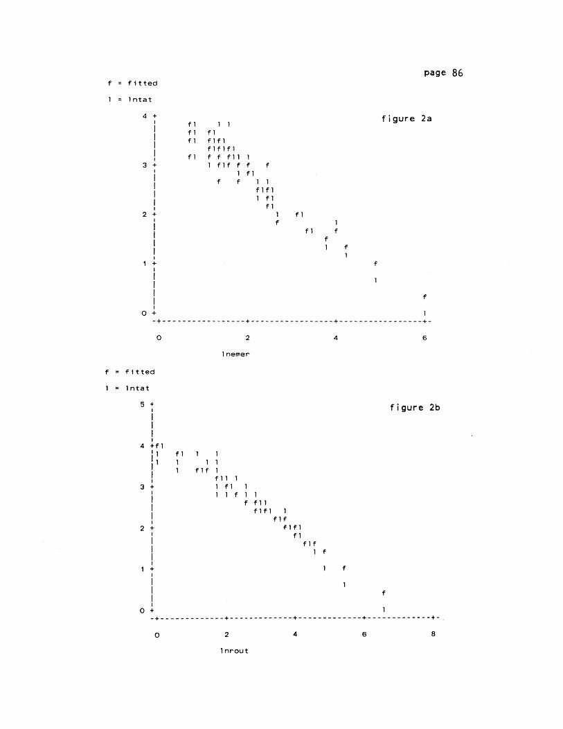
page 86f = fitted
1 = Intat
4 +
3 +
2 +
1+
0 +
f1fif I
f I
1 1fI
f f f I1 fif f
f f
O0
figure 2a
1f f
1 1
fl
f
2
fl
1fl
f
4 6
1 nemer
f = fitted
1 = Intat
+ figure 2b
+f 1'1 f1 1 1
' 1 1 1 11 flf 1
fl1 1+ 1 fl 1
11 ffif1 1
fif+ flfl
flfi f
lif
+ 1 f
+ 1------------------------------------------------------------
n 2 4 6 8
1 nrout
5
4
3
2
1
0
I
I

page 87f = fitted
1 = 1ntat
fl 1fI f 1f I f
f1 fl1 f1f fIf f I1 flI
f f 1 fIflf1 I
figure 2c
fIf II f
fI 1f If fI
4 +
3 +
2+
1+
0 +
f
2 4 6
inl icen
f = fitted
1 = 1ntat
1 fi1l 1 1fl fIf 1
f1l f1f fIf1f1
f fIf f1
figure 2d
f 11 fIff111 f 1
ff 1 1fl11if
f 11f 1
flfI f
1f
f
2 4 6
1nskil1
f1 f
1
0 8
4 +
3 +
2 +
i+
0+
0 8
1

page 88
BIBLIOGRAPHY
Allen, A.0.(1978) Probability, Statistics and Queueing TheoryNew York: Academic Press
Boston Housing Authority, "Monthly Management Report" Vol 1, 12/83, 1/84"Living Unit Inspections", Gilmore, D. I., 8/83"Maintenance Service", Gilmore, D. I., 3/84"Dallas Housing Authority Work Order Procedures"Gilmore, D. I., 9/83
"The New Work Order System", Friend, G., 3/84"Memorandum of Agreement with the BostonBuilding Trades Council", 1/84
Ferreira, J.(1973) Analysis of Public Systems, Ch. 15, MIT Press
Forthofer, R. N. & Lehnen, R. G.(1981)Categorical Data Approach,
Public Program Analysis: A NewBelmont, CA: Wadsworth
Hoos, I. R.(1972) Systems Analysis in Public Policy: A CritiqueBerkeley: UC Press
Kaplan, E. H. & Larson, R. C.(1981) "Decision-Oriented Approaches toProgram Evaluation", Operations Research Center, MIT
Larson, C. L. & Odoni, A. R.(1981) Urban Operations ResearchEnglewood Cliffs, NJ: Prentice Hall
Larson, R. C.(1978) "Improving the Effectiveness of New York City's 911"Operations Research Center, MIT
MIT, Laboratory of Architecture & Planning, Consistent System:"Elementary Statistical Analysis" 1980"CS Program Summaries" 1981"Elementary Janus Manual" 1978"Janus Reference Manual" 1982
Massey, F. J.(1951) "The Kolmogorov-Smirnov Test for Goodness of Fit"J. of Amer. Stat. Assoc. 46
Newell, G. F.(1971) Applications of Queueing Theory, London: Chapman & Hall
Saaty, T.(1961) Elements of Queueing Theory, New York: McGraw Hill
Stokey, E. & Zeckhauser, R.(1978) A Primer for Policy AnalysisNew York: Norton
Tufte, E. R.(1974) Data Analysis for Politics and Policy,
Englewood Cliffs, NJ: Prentice Hall
Weisberg, S.(1980) Applied Linear Regression, New York: Wiley