10.1.1.103.7728

Viscoplasticity model at ®nite deformations with combinedisotropic and kinematic hardening

Adnan Ibrahimbegovi�c a,*, Lot® Chor® b,1

a Ecole Normale Sup�erieure de Cachan=LMT, 61 av. du President Wilson, 94235 Cachan Cedex, Franceb Universit�e de Technologie de Compi�egne, Dept. GSM, bp-529, 60205 Compi�egne Cedex, France

Received 25 February 1999; accepted 25 October 1999

Abstract

In this work, we construct a phenomenological constitutive model of viscoplasticity at ®nite strains, which gener-

alizes the classical Perzyna or Duvaut±Lions models to ®nite strains. The latter is accomplished with a minimum

number of hypothesis, including the multiplicative decomposition of deformation gradient, a de®nition of the elastic

domain and ®nally a penalty-like, viscoplastic regularization of the principle of maximum plastic dissipation. The

model is extended to include the isotropic and kinematic hardening of Prager±Ziegler type. Numerical computation of

the viscoplastic ¯ow at ®nite strain is also discussed, along with the corresponding simpli®cation resulting from a

convenient choice of the logarithmic strain measure. Several illustrative numerical examples are presented in order to

demonstrate the ability of the proposed model to remove the de®ciencies of some currently used models. Ó 2000

Elsevier Science Ltd. All rights reserved.

Keywords: Viscoplasticity; Finite deformation; Kinematic hardening

1. Introduction

The main objective of this work is to develop a gen-

eral phenomenological model of plasticity at ®nite de-

formation, accounting for strain rate sensitivity as well as

isotropic and kinematic hardening e�ects. Since the

original viscoplasticity formulation of Ref. [1], the sub-

ject of hardening viscoplasticity in the regime of

small strains has fairly matured. Fundamental works of

Halphen and Nguyen [2], Moreau [3], Duvaut and Lions

[4], Nayroles [5] and Lemaitre and Chaboche [6], among

others, have provided a solid foundation for small strain

viscoplasticity in form of the variational inequality. This

point of view, strongly relying on convex analysis, has

also proved helpful in devising the computational strat-

egy based on the so-called catching up algorithm of

Moreau [3] and Nguyen [7], as an alternative to the radial

return algorithm of Wilkins [8] and Krieg and Krieg [9].

Extending these ideas to large strain analysis was

initially done in a somewhat ad-hoc manner, by using

hypo-plasticity models and simply replacing the stress

and strain from the small strain constitutive equation by

chosen stress and strain rates, respectively. It was soon

noticed that such an implementation leads to spurious

oscillations for some stress rates (e.g. Jaumann stress rate

in a simple shear test [10±12], potential problems with

kinematic hardening mechanics [13] and spurious energy

supply in a closed elastic strain path [14]. The main

reason for the forementioned de®ciencies of such a model

was traced to its incompatibility with the hyperelastic

behavior even in the absence of plastic deformation [15].

For this reason, the hypo-plasticity models of

this kind are currently getting abandoned in favor of

hyper-plasticity models, for which one can exploit the

kinematic hypothesis of Lee [16] and Mandel [17] on

multiplicative decomposition of deformation gradient in

Computers and Structures 77 (2000) 509±525

www.elsevier.com/locate/compstruc

* Corresponding author. Tel.: +33-1-4740-2239; fax: +33-1-

4740-2785.

E-mail address: [email protected] (A. IbrahimbegovicÂ).1 Graduate Research Assistant.

0045-7949/00/$ - see front matter Ó 2000 Elsevier Science Ltd. All rights reserved.

PII: S 0 0 4 5 - 7 9 4 9 ( 9 9 ) 0 0 2 3 2 - 1

elastic and inelastic part, to construct strain energy

function. The fact that one can construct the strain en-

ergy function for a large strain plasticity model was al-

ready recognized as early as 1965 [18]. However, it is

only with later works of Simo and Ortiz [19], Simo [20]

and Moran et al. [21], much inspired by related works of

Marsden and Hughes [22] on ®nite deformation elas-

ticity, that a sound formulation and numerical imple-

mentation of the ®nite deformation plasticity models

with strain energy are furnished. This was achieved at

the expense of raising signi®cantly the level of generality

and placing the developments in the framework of

manifolds. 2 The main advantage of the ®nite defor-

mation plasticity formulation of this kind with respect to

the hypo-plasticity formulation employed previously is

that the issue of stress or strain rates is completely cir-

cumvented by appealing to the notion of the Lee de-

rivative [22, p. 93].

It was shown more recently by Ibrahimbegovi�c [23]

that the complexity of tensor calculus on a manifold can

be signi®cantly reduced by extending to manifolds the

fundamental work of Hill [24] on the principal axis

representation of tensors, where manipulating the ten-

sors can be replaced by manipulating their principal

values, i.e. scalars. In order to simplify the numerical

implementation, the principal axis formulation of plas-

ticity can further be recast in the Euclidean setting, ei-

ther by choosing the unit matrix representation of the

metric tensor [25] or by assuming the Euclidean setting

at the outset [26]. It was also noted [27±30] that the

principal axis formulation in conjunction with the log-

arithmic ®nite strain measure can be used to formally

simplify the plastic ¯ow computation to the one, which

is employed in small strain case.

In this work, we take these considerations one step

further to develop a hardening viscoplasticity model. In

that respect, the contributions for which we believe to be

of special interest are

(i) A sound theoretical formulation of the ®nite de-

formation viscoplasticity model is developed from a

minimum number of hypotheses, including the multi-

plicative decomposition of deformation gradient, and a

general form of the strain energy constructed as an

isotropic function of the elastic strain measure. It is

shown that the standard thermodynamics consideration

and a penalty-like, viscoplastic regularization of the

principle of maximum plastic dissipation provide all the

corresponding constitutive and evolution equations for

the generalization of the classical models of Perzyna [1]

or Duvaut±Lions [4] to the ®nite strain regime.

(ii) The formulation is set in the space of principal

axis of the spatial strain measures, which splits the

geometrically nonlinear e�ects from the viscoplastic ¯ow

computation. The operator split method can be used to

exploit such a split and simplify the numerical imple-

mentation. In particular, choosing the logarithmic or

natural strain measure, the governing equations for the

viscoplastic ¯ow computation become formally the same

as those from small strain case. Due to isotropy of the

elastic response, the stress computation can also be

simpli®ed accordingly.

(iii) Careful thermodynamics consideration is given

to the isotropic and kinematic hardening phenomena,

with the latter generalizing the classical model of Prager

and Ziegler to ®nite strains. The principal axis setting

clearly illustrates the key feature of the kinematic

hardening model of this kind with the corresponding

strain-like hardening variable, which shares the same

eigenvectors with the viscoplastic strain.

The outline of this article is as follows: The governing

equations of the ®nite deformation perfect viscoplastic-

ity model are developed in Section 2 along with the

appropriate extensions of such model capable of han-

dling isotropic and kinematic hardening. In Section 3,

we discuss the numerical implementation of the model.

A number of selected numerical simulations are given in

Section 4. In Section 5, we give some closing remarks.

2. Theoretical formulation

2.1. Extending classical viscoplasticity to ®nite strains

We start our considerations by constructing a con-

venient extension of the classical Perzyna or Duvaut±

Lions-type, perfect viscoplasticity model to ®nite strain

regime. By generalizing the kinematic hypothesis of Lee

[16] and Mandel [17] to viscoplasticity, we assume that

the total deformation gradient, F, can be multiplica-

tively decomposed into elastic, Fe, and the viscoplastic

part, Fvp, i.e.

F � FeFvp: �1�

We note that Feÿ1 would unload elastically, the stress

in the neighborhood u�O�X�� in the deformed con®gu-

ration, which gives rise to a stress-free intermediate

con®guration. 3 On the contrary, Fvp acts as an internal

variable, which expresses the viscoplastic ¯ow or the

amount of dislocation of the crystal lattice. Therefore,

the process is de®ned as elastic if no change of Fvp would

take place.

2 See e.g. Ref. [22].

3 We note that the multiplicative decomposition of the

deformation gradient is de®ned only pointwise, so that the

intermediate `con®guration' does not necessarily represent a

collection of compatible neighborhoods.

510 A. Ibrahimbegovi�c, L. Chor® / Computers and Structures 77 (2000) 509±525

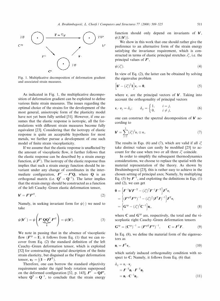
As indicated in Fig. 1, the multiplicative decompo-

sition of deformation gradient can be exploited to de®ne

various ®nite strain measures. The issues regarding the

optimal choice of the strains for the development of the

most general, anisotropic form of the plasticity model

have not yet been fully settled [31]. However, if one as-

sumes that the elastic response is isotropic, all the for-

mulations with di�erent strain measures become fully

equivalent [23]. Considering that the isotropy of elastic

response is quite an acceptable hypothesis for most

metals, we further pursue a development of one such

model of ®nite strain viscoplasticity.

If we assume that the elastic response is una�ected by

the amount of viscoplastic ¯ow, it further follows that

the elastic response can be described by a strain energy

function, w�Fe�. The isotropy of the elastic response thus

implies that such a strain energy function should be in-

variant under any change of coordinates in the inter-

mediate con®guration, Fe� ! FeQ, where Q is an

orthogonal matrix (i.e. QT � Qÿ1). The latter implies

that the strain energy should be constructed as a function

of the left Cauchy±Green elastic deformation tensor,

be � FeFeT: �2�

Namely, in seeking invariant form for w�� we need to

take

w�be�� w Fe QQT|�{z�}I

FeT

0@ 1A � w�be�: �3�

We note in passing that in the absence of viscoplastic

¯ow �Fvp � I�, it follows from Eq. (1) that we can re-

cover from Eq. (2) the standard de®nition of the left

Cauchy±Green deformation tensor, which is exploited

[32] for constructing the spatial description of the ®nite

strain elasticity, but disguised as the Finger deformation

tensor, eF � 12�1ÿ FFT�.

Therefore, one can borrow the standard objectivity

requirement under the rigid body rotation superposed

on the deformed con®guration [32, p. 143], Fe� � QFe,

where QT � Qÿ1, to conclude that the strain energy

function should only depend on invariants of be,

w�Ii�be��.We show in this work that one should rather give the

preference to an alternative form of the strain energy

satisfying the invariance requirement, which is con-

structed in terms of elastic principal stretches kei , i.e. the

principal values of Fe,

w�kei �: �4�

In view of Eq. (2), the latter can be obtained by solving

the eigenvalue problem

behÿ �ke

i �21imi � 0; �5�

where mi are the principal vectors of be. Taking into

account the orthogonality of principal vectors

mi � mj � dij; dij � 1; i � j;0; i 6� j;

��6�

one can construct the spectral decomposition of be ac-

cording to

be �X3

i�1

�kei �2mi mi: �7�

The results in Eqs. (6) and (7), which are valid if all kei

take distinct values can easily be modi®ed [25] to ac-

count for the case when two or all three kei coincide.

In order to simplify the subsequent thermodynamics

considerations, we choose to replace the spatial with the

material representation of the theory. As shown by

Ibrahimbegovi�c [23], this is rather easy to achieve in the

chosen setting of principal axes; Namely, by multiplying

Eq. (5) by Fÿ1, and exploiting the de®nitions in Eqs. (1)

and (2), we can get

0 � Fÿ1beFÿTh

ÿ �kei �2Fÿ1FÿT

iFTmi

� �FvpTFvp�ÿ1h

ÿ �kei �2�FTF�ÿ1

iFTmi

� Gvph

ÿ �kei �2Cÿ1

ini; �8�

where C and Gvp are, respectively, the total and the vi-

scoplastic right Cauchy±Green deformation tensors

Gvp � �Cvp�ÿ1 � �FvpTFvp�ÿ1; C � FTF: �9�In Eq. (8), we de®ne the material form of the eigenvec-

tors as

ni � FTmi; �10�which satisfy induced orthogonality condition with re-

spect to C; Namely, it follows from Eq. (6) that

dij � mi � mj

� FÿTni � FÿTnj

� ni � Cÿ1nj: �11�

Fig. 1. Multiplicative decomposition of deformation gradient

and associated strain measures.

A. Ibrahimbegovi�c, L. Chor® / Computers and Structures 77 (2000) 509±525 511

We can see that the material form of the eigenvalue

problem in Eq. (5) does not a�ect the values of the

elastic principal stretches. Consequently, neither does it

a�ect the chosen strain energy function constructed in

terms of principal stretches

w�kei � � w�C;Gvp�: �12�

The standard thermodynamics considerations [33±35]

and the regularized form of the principle of maximum

plastic dissipation are su�cient to provide all the gov-

erning equations for the perfect viscoplasticity model.

Namely, for the material representation of the strain

energy in Eq. (12), we can state a purely mechanical

form of the dissipation inequality

0 6 D :� S � 12

_Cÿ oot

w�C;Gvp�

� S

ÿ 2

owoC

!� 12

_Cÿ 2ow

oGvp �1

2_Gvp; �13�

where S is the second Piola±Kirchho� stress tensor

[22,32] which in the context of elasticity forms an ener-

gy-conjugate pair with the Green±Lagrange strain,

E � 12�Cÿ I�.

In an elastic process, where no change in Fvp or,

according to de®nition in Eq. (9), no change in Gvp takes

place � _Gvp � 0�, it holds that D � 0, so that we can

compute the second Piola±Kirchho� stress by a mere

function evaluation, since

D � 0 ) S � 2owoC

: �14�

In view of Eq. (12), the latter can also be expressed in

principal axes as

S � 2X3

i�1

owoke

i

okei

oC: �15�

The last term in Eq. (15) can be computed from the

directional derivative with respect to C of the eigenvalue

statement in Eq. (8), to get

0 �ÿ 2kei

okei

oC� dC

� �Cÿ1ni ÿ �ke

i �2oCÿ1

oCni

� Gvph

ÿ �kei �2Cÿ1

idni: �16�

Scalar multiplying the last expression by nj and making

use of the eigenvector orthogonality in Eq. (11), along

with the standard result, 4 �oCÿ1=oC� � dC � Cÿ1 dCCÿ1,

we obtain

okei

oC� ke

i

2Cÿ1ni Cÿ1ni; �17�

which can be exploited to simplify the principal axis

representation of the second Piola±Kirchho� stress in

Eq. (15) to get

S �X3

i�1

owoke

i

kei Cÿ1ni Cÿ1ni: �18�

This last result can also be interpreted as the spectral

decomposition of the second Piola±Kirchho� tensor with

si � owoke

i

kei �19�

as its principal values. The latter can be computed by

solving the eigenvalue problem

�Sÿ siCÿ1�ni � 0: �20�

The directional derivative of the eigenvalue statement in

Eq. (8) with respect to Gvp results with

0 � dGvpni ÿ 2kei

okei

oGvp � dGvp

� �Cÿ1ni

� Gvph

ÿ �kei �2Cÿ1

idni

�� nj

) okei

oGvp �1

2kei

ni ni: �21�

In view of the result in Eq. (17) and the last result, it

further follows that

okei

oC� Cÿ1 oke

i

oGvp Gvp: �22�

With this result on hand and the chain rule, we can

obtain that ow=oC � Cÿ1�ow=oGvp�Gvp, which allows us

to further simplify the dissipation inequality in Eq. (13)

for a viscoplastic process to get

0 < Dvp :� ÿCSGvpÿ1 � 12

_Gvp � ÿS � 12C _GvpGvpÿ1: �23�

In generalizing the classical viscoplasticity model of

over-stress type, we consider a process to be viscoplastic

for all the values of the stress outside the elastic domain

corresponding to a positive value of the function

/�S;C� � /�si� > 0: �24�The elastic domain is de®ned by the negative value of

Eq. (24), and its boundary is given by /�S;C� �/�si� � 0.

The evolution equation for the viscoplastic strain can

be deduced by appealing to the principle of maximum

plastic dissipation [36,37], which at a given deformed

con®guration (i.e. given value of �C) chooses the value of

stress, which would maximize the viscoplastic dissipation

outside of the elastic domain. The latter can be formu-

lated as an unconstrained minimization problem with

4 This result can easily be derived by computing the

directional derivative with respect to C of the identity I � Cÿ1C.


Hvp�S� � ÿDvp�S� �P / S; �C� ��

! min; �25�

where P�/�� is a penalty-like functional, which should

take zero value in the elastic domain and its boundary.

In accordance with the classical viscoplasticity models of

Perzyna [1] and Duvaut and Lions [4], the penalty-like

functional is chosen as

P�/�� 1

2g �/��2; / > 0;

0; / 6 0;

(�26�

where g is the viscosity parameter. It readily follows that

from Eq. (26) that the derivative of the chosen func-

tional can be written by using the Macauley bracket. 5

P0�/�� 1

gh/��i :�

1g /��; / > 0;

0; / 6 0:

(�27�

With this result on hand, the minimization problem in

(25) can be solved resulting in

0 � oHvp

oS:� 1

2C _GvpGvpÿ1 � 1

gh/i o/

oS; �28�

which provides the desired evolution equation for the

viscoplastic strain

_Gvp � ÿ2h/ig

Cÿ1 o/oS

Gvp: �29�

The last result can be further simpli®ed if one resorts to

the principal axis representation, namely, the directional

derivative of the eigenvalue statement in Eq. (20) can be

computed to give

0 � dSni ÿ osi

oS� dS

� �Cÿ1ni � S

� ÿ siCÿ1�dni

�� nj

) osi

oS� ni ni: �30�

In view of the principal axis representation of the

elastic domain in Eq. (24) and the last result a simple

application of the chain rule allows to recast the evolu-

tion equation for the viscoplastic strain as

_Gvp � ÿ2h/ig

X3

i�1

o/osi

Cÿ1ni

ni

!Gvp: �31�

Remark 1: isochoric viscoplastic ¯ow

If the boundary of the elastic domain is pressure in-

sensitive, so thatP3

i�1�o/=osi� � 0, one can show that

the viscoplastic deformation is isochoric. Namely, by

appealing to the notion of the exponential function of a

tensor [32] which states that the initial value problem

_X�0� � AX�0�; X�0� � I �32�

with A a given tensor, has exactly one solution

X�t� � exp�At� :�X1i�0

I

�� 1

n�tA�

�n

: �33�

This result can directly be applied to obtain the corre-

sponding exact solution of the evolution equation for

viscoplastic ¯ow in Eq. (31), after recalling that

Gvp�0� :� �FvpT�0�Fvp�0��ÿ1 � I, to get

Gvp�t� � exp

"ÿ 2h/ig

X3

i�1

o/osi

Cÿ1ni ni

#: �34�

It can further be shown [32, p. 227] that

det�exp�At�� exp�tr�At��, which in application to Eq.

(34) leads to

det�Gvp�t�� exp tr

"(ÿ 2h/ig

X3

i�1

o/osi

Cÿ1ni

� ni

�#)

� exp

(ÿ 2h/ig

X3

i�1

o/osi

): �35�

For any pressure insensitive form of the elastic domain

withP3

i�1�o/=osi� � 0, it follows from the last result

that

det Gvp�t� � 1 �36�

or, in other words, that the viscoplastic deformation

tensor is a unimodular tensor. In view of de®nition in

Eq. (9), it further follows that

det Fvp�t� � 1; �37�

which implies that the viscoplastic ¯ow is isochoric, or

that there is no change in plastic volume. We note in

closing this remark that the pressure insensitive form of

/�� can be de®ned in terms of deviatoric principal val-

ues

/�si�; si � si ÿ 1

3

X3

k�1

sk : �38�

2.2. Including isotropic and kinematic hardening

In order to increase the predictive capabilities of the

perfect viscoplasticity model at ®nite strains, we set in

this section to include the internal variables which could

handle the isotropic and kinematic hardening phenom-

ena. In particular, a strain-like scalar variable n is in-

troduced to handle the increase in since of the elastic

domain, i.e. isotropic hardening, and the strain-like

tensor variable N is introduced to handle the eventual

translation of the elastic domain.

5 The Macauley bracket ®lters out only the positive value of

function; i.e. hxi � x, x > 0 and hxi � 0, x 6 0.


The strain energy function should thus be generalized

to include these two hardening variables as

~w�C;Gvp;N; n�: �39�For the subsequent considerations, we choose the

kinematic hardening model, which represents an ap-

propriate generalization to the ®nite strain regime of the

classical Prager±Ziegler kinematic hardening rule [37, p.

137], in that the kinematic hardening variable N is pro-

portional to the viscoplastic strain Gvp, i.e. N � cGvp,

where c is a constant. In the present setting of the

principal axes the latter can be formulated by postulat-

ing that N and Gvp share the same eigenvectors. There-

fore, in view of the results in Eqs. (8) and (9), we can

write

�Nÿ �zi�2Cÿ1�ni � 0; �40�where zi are the principal values of strain-like kinematic

hardening tensor.

With this result on hand, one can also provide the

principal axis representation of the strain energy as

w�kei ; zi; n� �41�

with respect to the principal axes ni shared by both Gvp

and N. Similar representations can also be given for the

new de®nition of the elastic domain in terms of

~/�C;S;A; q� � /�si; ai; q�; �42�where q is the isotropic hardening variable, conjugate to

n, whereas A is the kinematic hardening variable, i.e. the

back stress, with its principal values given as ai. In other

words, we can write that

�Aÿ aiCÿ1�ni � 0: �43�

The dissipation inequality in Eq. (13) corresponding to

the new form of the strain energy can be rewritten as

0 6 D :�S � 12

_Cÿ oot

~w�C;Gvp;N; n�

� S

ÿ 2

o ~woC

!� 12

_Cÿ 2o ~w

oGvp �1

2_Gvp

ÿ 2o ~woN� 12

_Nÿ o ~won� n: �44�

In an elastic process, where no change takes place

regarding internal variables, i.e. _Gvp � 0 � _Fvp � 0�,_N � 0 and n � 0, the dissipation vanishes, so that, we

again recover the constitutive equations for the second

Piola±Kirchho� stress as already obtained in Eq. (14).

Further, we can also de®ne the stress-like isotropic

hardening variables q by its constitutive equation

q � ÿ o ~won: �45�

For the selected generalization of the Prager±Ziegler

kinematic hardening model, the constitutive equations

for the back stress can be obtained by making use of the

principal axis representation as

A �X3

i�1

2owozi

ozi

oC

�X3

i�1

owozi

ziCÿ1ni Cÿ1ni; ai � ow

ozizi: �46�

In view of results in Eqs. (40) and (43) and previously

derived similar conclusion in Eq. (22), we can write that

ozi

oC� Cÿ1 ozi

oNN; �47�

which can be used to obtained a reduced form of the

dissipation inequality valid for a viscoplastic process

0 < Dvp :� ÿS � 12C _GvpGvpÿ1 ÿ A � 1

2C _NNÿ1 � qn: �48�

The principle of maximum plastic dissipation can

now be reformulated by using the corresponding form of

the elastic domain in Eq. (42), providing the evolution

equations of the internal variables

0 � oHvp

oS:� 1

2C _GvpGvpÿ1 � 1

gh ~/i o

~/oS

) _Gvp � ÿ2h ~/ig

Cÿ1 o ~/oS

Gvp; �49a�

0 � oHvp

oA:� 1

2C _NNÿ1 � 1

gh ~/i o

~/oA

) _N � ÿ2h ~/ig

Cÿ1 o ~/oA

N; �49b�

0 � oHvp

oq:� ÿn� 1

gh ~/i o

~/oq) _n � h

~/ig

o ~/oq: �49c�

The principal representation of the evolution equation

(49a) again takes the form as given in Eq. (31), whereas

the one in Eq. (49b) reduces to

_N � ÿ2h/ig

X3

i�1

o/oai

Cÿ1ni

ni

!N: �50�

Remark 2: kinematic hardening isochoric variable and

deviatoric back stress

The conclusion drawn in Remark 1 can readily be

extended to internal variables governing proposed ki-

nematic hardening model of the Prager±Ziegler type.

Namely, if the back stress featuring in the de®nition of

the elastic domain in Eq. (42) is deviatoric, with its

principal values a1 � a2 � a3 � 0, the corresponding

strain-like kinematic hardening variable N is a unimod-

ular tensor.


Namely, by making use again of the exponential

function to compute the exact solution to evolution

equation (50) we get

N�t� � exp

"ÿ 2h/ig

X3

i�1

o/oai

Cÿ1ni

� ni

�#; �51�

which further implies that

det N�t� � exp tr

"(ÿ 2h/ig

X3

i�1

o/oai

Cÿ1ni

� ni

�#)

� exp

8>>><>>>:ÿ 2h/ig

X3

i�1

o/oai|��{z��}

�0

9>>>=>>>;� 1: �52�

2.3. Spatial description

All the governing equations of the proposed ®nite

strain viscoplasticity model with combined isotropic and

kinematic hardening can also be cast in spatial descrip-

tion, which turns out to provide a more convenient basis

for an e�cient numerical implementation. This is ac-

complished simply by exploiting the relationship be-

tween the spatial and the material form of the principal

vectors in Eq. (12) and reversing the operation that lead

us to replace the eigenvalue problem in Eq. (5) by its

counterpart in Eq. (8).

To that end, one ®rst have to de®ne the spatial rep-

resentation of the second Piola±Kirchho� stress in terms

of the Kirchho� stress

s � FSFT; �53�

which shares the same principal values si; Namely, from

Eq. (20) we can get

0 � Sÿ ÿ siC

ÿ1�ni jF�

� FSFT|��{z��}s

24 ÿ siF�FTF�ÿ1FT

#FÿTni|��{z��}

mi

� �sÿ si1�mi: �54�

The stress constitutive Eq. (18) can similarly be modi®ed

to get

s :� FSFT �X3

i�1

owoke

i

kei F�FTF�ÿ1

ni F�FTF�ÿ1ni

�X3

i�1

owoke

i

kei mi mi ) si � ow

okei

kei : �55�

The kinematic hardening strain-like variable can also be

written in spatial description with

z � FNFT; �56�which, by exploiting the result in (40), can easily be

shown to have the same principal vectors, since

0 � Nÿ ÿ z2

i Cÿ1�ni jF�

� FNFT|��{z��}z

24 ÿ z2i F�FTF�ÿ1FT

35FÿTni|��{z��}mi

� �zÿ z2i 1�mi: �57�

A similar spatial representation can be provided for

back-stress, since from Eq. (46) we get

a :� FAFT �X3

i�1

owozi

ziF�FTF�ÿ1ni F�FTF�ÿ1

ni

�X3

i�1

owozi

zimi mi ) ai � owozi

zi: �58�

By making use of the foregoing results we can ®nally

provide the spatial description of the evolution equa-

tions. In particular, it follows from Eq. (8) that one can

de®ne

be � FGvpFT: �59�The time derivative of the last equation can be readily

computed to obtain

_be � _FFÿ1FGvpFT � FGvpFTFÿT _FT � F _GvpFT

� lbe � belT � F _GvpFT; �60�where l � _FFÿ1 is the spatial velocity gradient. With this

result on hand we can provide the spatial representation

of the evolution Eq. (29) as

_be ÿ lbe ÿ belT � F _GvpFT

� ÿ2h/ig

X3

i�1

o/osi

FCÿ1ni niGvpFT

� ÿ2h/ig

X3

i�1

o/osi

F�FTF�ÿ1FT|��{z��}I

mi

mi FGvpFT|��{z��}be

� ÿ2h/ig

X3

i�1

o/osi

mi

mi

!be; �61�

where the results in Eqs. (12) and (59) were used. A

similar transformation can be performed for the evolu-

tion equation of kinematic hardening variable in Eq.

(50) to obtain

_zÿ lzÿ zlT � ÿ2h/ig

X3

i�1

o/oai

mi

mi

!z: �62�


3. Numerical implementation

In summary of considerations given in the previous

section, we note that the internal state variables for the

presented viscoplasticity model in spatial representation

are: the left Cauchy±Green elastic deformation tensor,

be, the kinematic hardening tensor, z, and the isotropic

hardening scalar variable, n. The list of state variables

should be completed by the position vector in the de-

formed con®guration, u, which is used to compute the

total deformation gradient

F � �u;1 u;2 u;3�; �63�

where u;i denotes the partial derivative of the position

vector with respect to the corresponding coordinate, xi.

The central problem of the computational visco-

plasticity reduces to tracing the time histories of the state

variables: u�t�, be�t�, z�t� and n�t� in the time interval of

interest. The central problem is well posed, and it can be

solved by integrating the evolution equations in Eqs.

(49c), (61) and (62), accompanied by the weak form of

momentum balance equations. The latter is obtained by

using the principle of virtual power [38] as

G�u; be; z; n; _u� :�ZB

s � dÿ Gext � 0; �64�

where B is the material domain occupied by the body

and Gext is the external virtual power. The integral in Eq.

(64) is computed by using the ®nite element method and

the quadrature formulae (Gauss quadrature, [39,40]),

which, as elaborated upon by Ibrahimbegovi�c et al. [41],

allows the computation of the state variables to be re-

duced to a single quadrature point at the time. Consid-

ering further that one-step solution schemes are typically

used to carry out the computation, the central problem

of computational viscoplasticity can be restated as fol-

lows:

Central problem in computational viscoplasticity (8quadrature point)

Given : un � u�tn�; ben � be�tn�; zn � z�tn�;

nn � n�tn�;Dt � tn�1 ÿ tn > 0;

compute : un�1 � u�tn�1�; ben�1 � be�tn�1�;

zn�1 � z�tn�1�; nn�1 � n�tn�1�:

We note in passing that after having computed the

state variables at time tn�1, we can recover the corre-

sponding values of dependent variables: the stress ten-

sor, sn�1, the back-stress, an�1, the isotropic hardening

stress-like variable, qn�1, simply by using the constitutive

Eqs. (55), (58) and (45), respectively.

The central problem of computational viscoplasticity

is composed of a large number of local equations (one

set of internal variable evolution equations for each

quadrature point) and a single set of global equilibrium

Eq. (64). As ®rst shown by Simo and Ortiz [19], such a

structure can be exploited to simplify the computation

by employing the operator split procedure to separate

the local (pertaining to a quadrature point) and global

computational tasks.

3.1. Internal variable computations

For the purpose of the discussion to follow, we as-

sume that the position vector at time tn�1, un�1, is ob-

tained, by solving the momentum balance Eq. (64). This

can be carried out either by a direct or an iterative

method, independent on local solution step. We recall

again that the latter is the only global computation,

which a�ects all the displacement degrees of freedom

simultaneously. The remaining local computation can

then be started to obtain the corresponding values of

internal variables, by integrating the evolution Eqs.

(49c), (61) and (62). To this end, we have to examine two

possibilities. A simpler one is when the process remains

elastic i.e. h/i � 0 leading to

_be ÿ lbe ÿ belT � 0; be�0� � ben; �65�

_zÿ lzÿ zlT � 0; z�0� � zn; �66�

_n � 0; n�0� � nn; �67�

which de®nes the so-called elastic trial step.

It is immediately apparent that the exact solution of

the last equation can be obtained as

ntrialn�1 � nn: �68�

Although it is somewhat less apparent, we can also ob-

tain closed-form solutions for Eqs. (65) and (66).

Namely, by exploiting the result in Eq. (59), for a ®xed

value of the viscoplastic deformation, �Gvp, Eq. (65) can

be rewritten as

_be � oot

FGvpFT� � ��

�Gvp ; be�0� � ben :� FnGvp

n FTn :

�69�

We recall again the chosen ®xed value of the plastic

deformation is consistent with the assumption of the

trial step being elastic. By introducing the relative de-

formation gradient

f n�1 � Fn�1Fÿ1n ; �70�

the exact solution for the elastic trial left Cauchy±Green

strain can be obtained

be;trialn�1 � Fn�1Gvp

n FTn�1

� f n�1ben f T

n�1: �71�


The computed value of the elastic strain is used to

devise the corresponding form of the eigenvalue problem

in Eq. (5),

be;trialn�1

hÿ �ke;trial

i;n�1 �21imtrial

n�1 � 0 �72�

leading to the trial values of elastic principal stretches,

ke;triali;n�1 , and the trial principal vectors, mtrial

n�1. The same

principal vectors are shared by the trial value of the

kinematic hardening tensor, ztrialn�1, while its principal

values are those from the previous step, ztriali;n�1 � zi;n.

Making use of the results in Eqs. (55), (58) and (45)

we can compute the corresponding trial values of the

Kirchho� stress, striali;n�1, and the back stress, atrial

i;n�1, and

isotropic hardening stress-like variable qtrialn�1. If the value

of / computed from Eq. (42) for so obtained trial values

is indeed negative or zero, i.e. if /�striali;n�1; a

triali;n�1; q

trialn�1� 6 0,

our guess for h/i � 0 was correct and the trial state can

be accepted as the ®nal state at time tn�1.

In the opposite case, if the trial value of / is positive,

we need to compute the true values of state variables

corresponding to modi®ed evolution equations

_be � ÿ 2

gh/i

X3

i�1

o/osi

mi

mi

!be; be�0� � be;trial

n�1 ; �73�

_z � ÿ 2

gh/i

X3

i�1

o/oai

mi

mi

!z; z�0� � ztrial

n�1; �74�

_n � h/ig

o/oq; n�0� � ntrial

n�1: �75�

We note that, in the spirit of the operator split method,

this kind of computation carries on from the computed

trial values.

An approximate ®rst-order solution to Eq. (75) can

be obtained by using the implicit, backward-Euler

scheme leading to

nn�1 � ntrialn�1 � cn�1

o/oq

��n�1

; �76�

where we denoted

cn�1 � h/n�1iDtg: �77�

Approximate ®rst-order solutions are also sought to

the evolution Eqs. (73) and (74), but as opposed to using

the backward-Euler scheme the exponential approxi-

mation is employed, as proposed earlier by Weber and

Anand [27], to get

ben�1 �

X3

i�1

exp

�"ÿ 2cn�1

o/osi

�mi;n�1 mi;n�1

#be;trial

n�1 ;

�78�

zn�1 �X3

i�1

exp

�"ÿ 2cn�1

o/oai

�mi;n�1 mi;n�1

#ztrial

n�1;

�79�where the orthogonality of the eigenvectors was ex-

ploited.

Further, from eigenvalue problems (5) and (57) writ-

ten at time tn�1, we can obtain the spectral decomposition

of the left Cauchy±Green elastic deformation tensor

ben�1 �

X3

i�1

�kei;n�1�2mi;n�1 mi;n�1 �80�

and the kinematic hardening strain tensor

zn�1 �X3

i�1

�zi;n�1�2mi;n�1 mi;n�1: �81�

Similar results can be written for the trial values of the

elastic strain and kinematic hardening variable, i.e.

be;trialn�1 �

X3

i�1

ke;triali;n�1

� �2

mtriali;n�1 mtrial

i;n�1; �82�

ztrialn�1 �

X3

i�1

ztriali;n�1

� �2

mtriali;n�1 mtrial

i;n�1: �83�

With these results on hand, we can devise the prin-

cipal axis representation of the exponential approxima-

tions (78) and (79). The latter, along with the uniqueness

of the spectral decomposition, implies that the trial and

®nal eigenvectors coincide, i.e.

mi;n�1 � mtriali;n�1 �84�

and that the trial values of elastic principal stretches and

kinematic hardening variables ought to be modi®ed ac-

cording to

�kei;n�1�2 � ke;trial

i;n�1

� �2

exp

�ÿ 2cn�1

o/osi

��n�1

�; i � 1; 2; 3

�85�

�zi;n�1�2 � ztriali;n�1

� �2

exp

�ÿ 2cn�1

o/oai

��n�1

�; i � 1; 2; 3:

�86�Introducingtheprincipal elastic logarithmicstretcheswith

�ei;n�1 � ln �ke

i;n�1�; �e;triali;n�1 � ln �ke;trial

i;n�1 � �87�

and the principal kinematic hardening logarithmic

strains with

ji;n�1 � ln �zi;n�1�; jtriali;n�1 � ln �ztrial

i;n�1� �88�

and taking logarithm at both sides of Eqs. (85) and (86),

we obtain


�ei;n�1 � �e;trial

i;n�1 ÿ cn�1

o/osi

��n�1

; i � 1; 2; 3; �89�

ji;n�1 � jtriali;n�1 ÿ cn�1

o/oai

��n�1

; i � 1; 2; 3 �90�

Therefore, with the present principal axis formula-

tion of the ®nite deformation viscoplasticity, we recover

formally the same structure of the internal variable up-

dates as the one from the small deformation theory,

since the multiplicative updates can be replaced by the

additive ones.

In particular, following Ibrahimbegovi�c et al. [41],

the viscoplastic ¯ow computation can be carried out in a

systematic manner by grouping together the results in

Eqs. (76), (77), (89) and (90) to get

rn�1 :��e

i;n�1 ÿ �e;triali;n�1 � cn�1osi/n�1

ÿ gDt cn�1 � /n�1

ji;n�1 ÿ jtriali;n�1 � cn�1oai/n�1

ÿnn�1 � nn � cn�1oq/n�1

8>><>>:9>>=>>; � 0; i � 1; 2; 3:

�91�

In Eq. (91), we have to solve a set of nonlinear al-

gebraic equations with cn�1, nn�1, �ei;n�1 and ji;n�1,

(i � 1; 2; 3) as unknowns. As shown in the next section,

for certain forms of /, such a computation can be per-

formed in a very e�cient manner, by reducing the sys-

tem to a single scalar equation, which is solved

iteratively.

Once such iterative procedure has converged, we can

recover the corresponding values of the elastic strains by

reversing the procedure in Eqs. (87) and (80)

ben�1 �

X3

i�1

�exp��ei;n�1��2mtrial

i;n�1 mtriali;n�1 �92�

as well as the kinematic hardening variable by making

use of the results in Eqs. (88) and (81)

zn�1 �X3

i�1

�exp�ji;n�1��2mtriali;n�1 mtrial

i;n�1: �93�

The corresponding values of the Kirchho� stress and the

back stress and isotropic hardening variables can also be

obtained from the constitutive equations in (55) and

(58), respectively.

3.2. Model problem: ®nite strain version of classical

Perzyna or Duvaut±Lions viscoplasticity

The classical form of the elastic domain, corre-

sponding to J2-¯ow theory, can readily be adapted to

the present model. If we ®rst consider the perfect vi-

scoplasticity case, we can write

/�~si� :� ~s21

�� ~s2

2 � ~s23

�1=2

ÿ��23

qsy ; �94�

where ~si � si ÿ 13

P3k�1 sk

� �and sy is the elasticity limit

for a uniaxial stress state. It is easy to see that such a

form of / is pressure insensitive, withP3

i�1�o/=osi� � 0,

which according to Remark 1 will result in isochoric

viscoplastic ¯ow. If we take into account the isotropic

and kinematic hardening of Prager±Ziegler type, we

should modify / in Eq. (94) as

/�~si; ai; q� :� �~s1

h� a1�2 � �~s2 � a2�2 � �~s3 � a3�2

i1=2

ÿ��23

q�sy ÿ q�: �95�

The strain energy is chosen as a function of the loga-

rithmic strain measures, by separating the isochoric

(viscoplastic-strain-producing) part, form the spherical

part;

w�J e; ~kei ; zi; n� :� 1

2B�ln J e�2 � 1

22l �ln ~ke

1�2h

� �ln ~ke2�2 � �ln ~ke

3�2i� 1

2

2H3

� �ln z1�2h

� �ln z2�2 � �ln z3�2i

� v�n�; �96a�

where B is the bulk modulus, l is the shear modulus, H

is the kinematic hardening modulus and v�n� is the

chosen (nonlinear) law for isotropic hardening. In Eq.

(96a), we denoted

J e � ke1k

e2k

e3;

~kei � �J e�ÿ1=3

so that ~ke1~ke

2~ke

3 � 1: �96b�As shown by Ibrahimbegovi�c et al. [41], the visco-

plastic ¯ow computation (at each Gauss quadrature

point) can be reduced for such a model to a single

nonlinear algebraic equation in cn�1.

The iterative solution for this equation makes use

at each iteration �k� of the corresponding linearized

form

2l

�� 2

3k0�n�k�n�1�h

� Hi� g

Dt

�Dc�k�n�1 � /�k�n�1 ÿ

gDt

c�k�n�1:

�97�The stress computation can also be simpli®ed due to

a particular choice of the strain energy function in Eq.

(96a); Namely, by making use of one results [23]

oJ e=obe � 12J ebeÿ1, the spherical part of stress is com-

puted as

�s � 2ow��oJ e

oJ e

obe be

� ow��oJ e

J e1: �98�


Similarly, it can easily be shown from Eqs. (5) and (96b)

that ~kei are the principal values of the unimodular part of

be, denoted as ~be � �J e�ÿ2=3be

~behÿ �~ke

i �21imi � 0: �99�

The deviatoric part of stress can then be computed as

~s � 2ow��o~ke

i

o~kei

~be

o~be

obe be

� 2ow��o~ke

i

1

2~kei

mi mi�J e�ÿ2=31

�ÿ 1

3be beÿ1

�be

� ow��o~ke

i

1

~kei

mi mi�23

be�: �100�

4. Numerical examples

In this section, we present several illustrative results

of numerical simulations. All the computations are

performed by a research version of the computer pro-

gram FEAP, written by Prof. R.L. Taylor at UC

Berkeley [39]. We employ a 4-node element, enriched by

a set of incompatible modes, as described in a recent

work of Ibrahimbegovi�c and Gharzeddine [18].

4.1. Stress solution for a closed elastic strain path

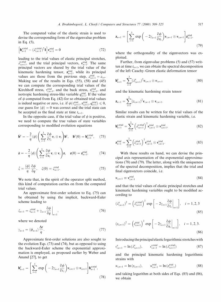
This example is adopted from a work of Koji�c and

Bathe [14]. It considers a square block of elastic material

(Fig. 2) subjected to a homogeneous deformation ®eld,

which starts from initially stress-free reference con®gu-

ration, followed by uniform extension, simple shear,

uniform compression and ®nal return to the initial form.

By considering that the material is hyperelastic, no re-

sidual stress should be found at the end of such a closed

elastic strain path, regardless of a particular order of

elementary deformations.

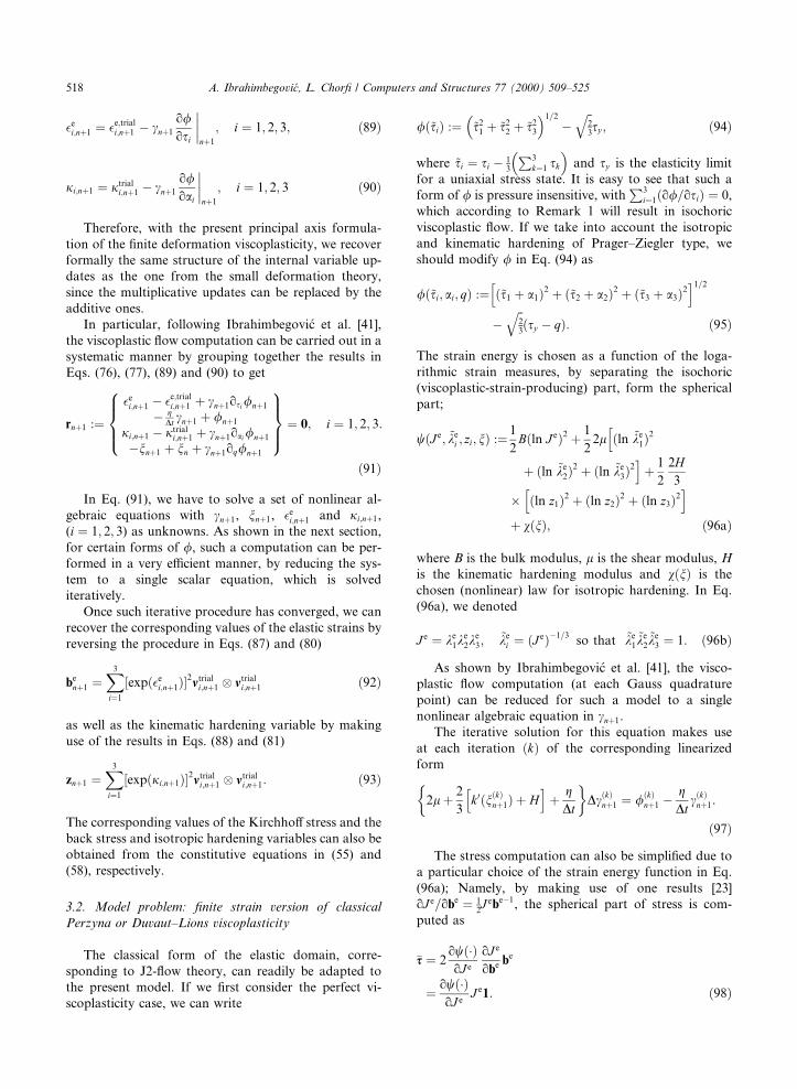
However, it was shown by Koji�c and Bathe [14] that

an often used constitutive model, employing the linear

elastic relationship between the Jaumann rate of the

Cauchy stress 6 and velocity strain tensors, is not capable

of reproducing this results. It leads instead to a residual

(homogeneous) stress ®eld, which depends on relative

values of the applied extension and shear (Fig. 3).

In contrast to this erroneous result obtained by the

Jaumann stress rate model, the present formulation

leads the exact response of zero residual stress ®eld. The

computation con®rming this kind of behavior is carried

out on a single 4-node element.

Fig. 2. Closed elastic strain path: problem description ± states

of deformations.

6 The Jaumann rate of the Cauchy stress is de®ned as

rr � _rÿ wr� rw, where w � 1

2�lÿ lT�. Fig. 3. Closed elastic strain path: residual stress.


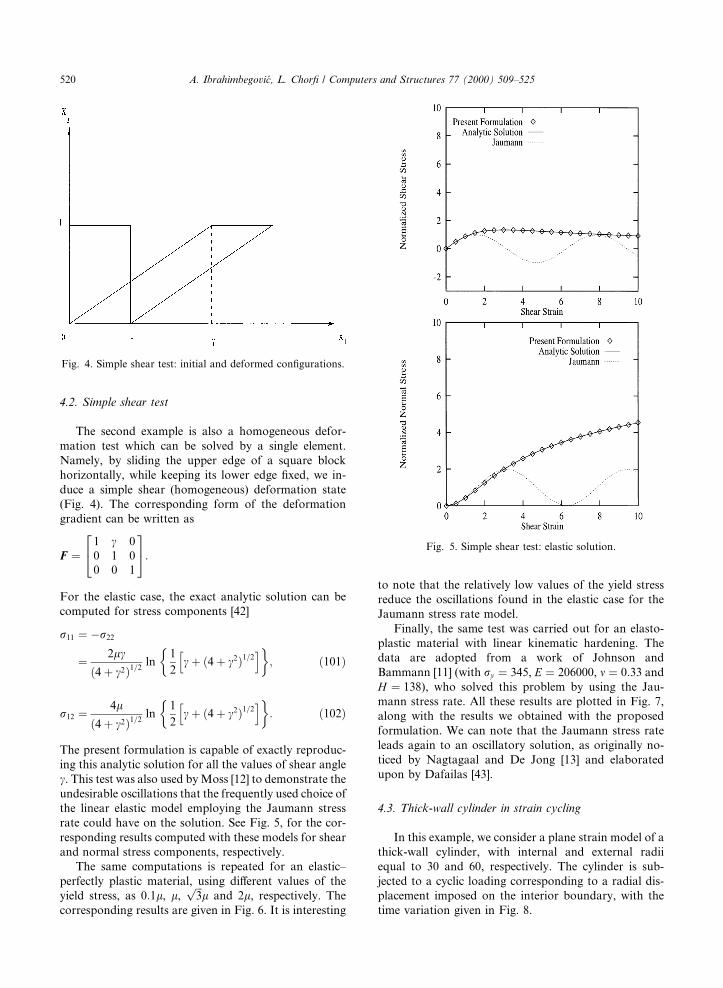
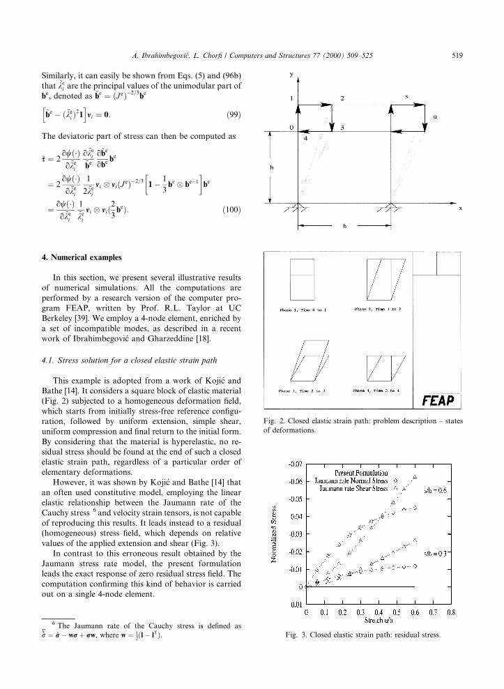
4.2. Simple shear test

The second example is also a homogeneous defor-

mation test which can be solved by a single element.

Namely, by sliding the upper edge of a square block

horizontally, while keeping its lower edge ®xed, we in-

duce a simple shear (homogeneous) deformation state

(Fig. 4). The corresponding form of the deformation

gradient can be written as

F �1 c 00 1 00 0 1

24 35:For the elastic case, the exact analytic solution can be

computed for stress components [42]

r11 � ÿr22

� 2lc

�4� c2�1=2ln

1

2ch�� 4� c2�1=2

i�; �101�

r12 � 4l

�4� c2�1=2ln

1

2ch�� 4� c2�1=2

i�: �102�

The present formulation is capable of exactly reproduc-

ing this analytic solution for all the values of shear angle

c. This test was also used by Moss [12] to demonstrate the

undesirable oscillations that the frequently used choice of

the linear elastic model employing the Jaumann stress

rate could have on the solution. See Fig. 5, for the cor-

responding results computed with these models for shear

and normal stress components, respectively.

The same computations is repeated for an elastic±

perfectly plastic material, using di�erent values of the

yield stress, as 0:1l, l,��3p

l and 2l, respectively. The

corresponding results are given in Fig. 6. It is interesting

to note that the relatively low values of the yield stress

reduce the oscillations found in the elastic case for the

Jaumann stress rate model.

Finally, the same test was carried out for an elasto-

plastic material with linear kinematic hardening. The

data are adopted from a work of Johnson and

Bammann [11] (with ry � 345, E � 206000, m � 0:33 and

H � 138), who solved this problem by using the Jau-

mann stress rate. All these results are plotted in Fig. 7,

along with the results we obtained with the proposed

formulation. We can note that the Jaumann stress rate

leads again to an oscillatory solution, as originally no-

ticed by Nagtagaal and De Jong [13] and elaborated

upon by Dafailas [43].

4.3. Thick-wall cylinder in strain cycling

In this example, we consider a plane strain model of a

thick-wall cylinder, with internal and external radii

equal to 30 and 60, respectively. The cylinder is sub-

jected to a cyclic loading corresponding to a radial dis-

placement imposed on the interior boundary, with the

time variation given in Fig. 8.

Fig. 5. Simple shear test: elastic solution.

Fig. 4. Simple shear test: initial and deformed con®gurations.


Making use of the symmetry of the structure and the

loading, the ®nite element model is constructed for a

quarter of the cylinder only (Fig. 9). The model consists

of 36 4-node elements with incompatible modes [25].

The material is considered to be elastic±viscoplastic,

with Young's modulus E � 2100 and Poisson's ratio

m � 0:33. Both kinematic hardening, with H � 5, and

isotropic hardening, are used. The latter is chosen as an

exponential-type saturation hardening model with

k�n� � �r1 ÿ ry��1ÿ eÿbn� � Kn;

where r1 � 60, ry � 30, K � 5 and b � 0:5. Two dif-

ferent values of viscosity parameter are chosen: g � 10,

for a viscoplastic behavior, and g � 10ÿ10, which basi-

cally reduces to rate-independent plastic behavior. The

computed numerical results are presented in Fig. 10, in

terms of pressure±displacement diagram. We can see

that from the chosen values of the viscosity parame-

ter the viscous e�ects are not very pronounced. In

Fig. 7. Simple shear test: kinematic hardening solution.

Fig. 8. Imposed radial displacement time history.

Fig. 9. Finite element model for thick cylinder.

Fig. 6. Simple shear test: elastic±perfectly plastic solution.


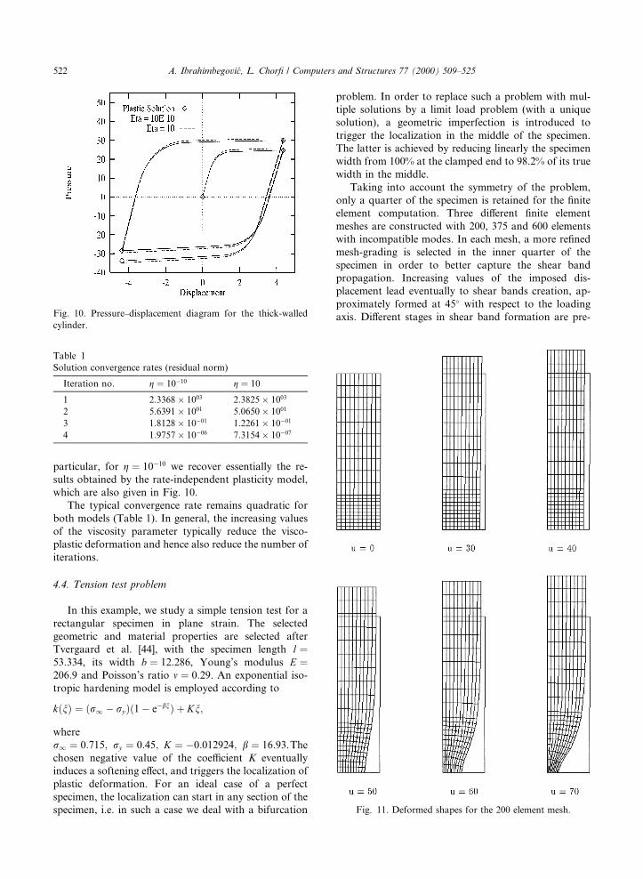
particular, for g � 10ÿ10 we recover essentially the re-

sults obtained by the rate-independent plasticity model,

which are also given in Fig. 10.

The typical convergence rate remains quadratic for

both models (Table 1). In general, the increasing values

of the viscosity parameter typically reduce the visco-

plastic deformation and hence also reduce the number of

iterations.

4.4. Tension test problem

In this example, we study a simple tension test for a

rectangular specimen in plane strain. The selected

geometric and material properties are selected after

Tvergaard et al. [44], with the specimen length l �53:334, its width b � 12:286, Young's modulus E �206:9 and Poisson's ratio m � 0:29. An exponential iso-

tropic hardening model is employed according to

k�n� � �r1 ÿ ry��1ÿ eÿbn� � Kn;

where

r1 � 0:715; ry � 0:45; K � ÿ0:012924; b � 16:93.The

chosen negative value of the coe�cient K eventually

induces a softening e�ect, and triggers the localization of

plastic deformation. For an ideal case of a perfect

specimen, the localization can start in any section of the

specimen, i.e. in such a case we deal with a bifurcation

problem. In order to replace such a problem with mul-

tiple solutions by a limit load problem (with a unique

solution), a geometric imperfection is introduced to

trigger the localization in the middle of the specimen.

The latter is achieved by reducing linearly the specimen

width from 100% at the clamped end to 98.2% of its true

width in the middle.

Taking into account the symmetry of the problem,

only a quarter of the specimen is retained for the ®nite

element computation. Three di�erent ®nite element

meshes are constructed with 200, 375 and 600 elements

with incompatible modes. In each mesh, a more re®ned

mesh-grading is selected in the inner quarter of the

specimen in order to better capture the shear band

propagation. Increasing values of the imposed dis-

placement lead eventually to shear bands creation, ap-

proximately formed at 45� with respect to the loading

axis. Di�erent stages in shear band formation are pre-

Fig. 11. Deformed shapes for the 200 element mesh.

Table 1

Solution convergence rates (residual norm)

Iteration no. g � 10ÿ10 g � 10

1 2:3368� 1003 2:3825� 1003

2 5:6391� 1001 5:0650� 1001

3 1:8128� 10ÿ01 1:2261� 10ÿ01

4 1:9757� 10ÿ06 7:3154� 10ÿ07

Fig. 10. Pressure±displacement diagram for the thick-walled

cylinder.


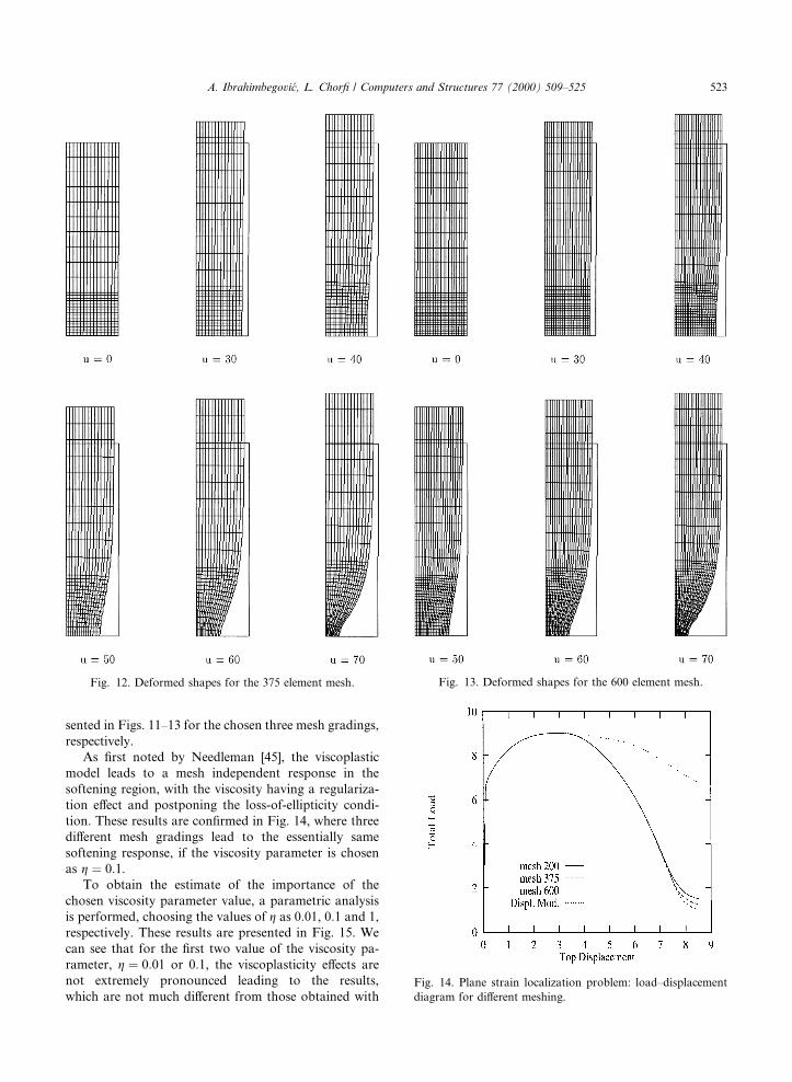
sented in Figs. 11±13 for the chosen three mesh gradings,

respectively.

As ®rst noted by Needleman [45], the viscoplastic

model leads to a mesh independent response in the

softening region, with the viscosity having a regulariza-

tion e�ect and postponing the loss-of-ellipticity condi-

tion. These results are con®rmed in Fig. 14, where three

di�erent mesh gradings lead to the essentially same

softening response, if the viscosity parameter is chosen

as g � 0:1.

To obtain the estimate of the importance of the

chosen viscosity parameter value, a parametric analysis

is performed, choosing the values of g as 0:01, 0:1 and 1,

respectively. These results are presented in Fig. 15. We

can see that for the ®rst two value of the viscosity pa-

rameter, g � 0:01 or 0:1, the viscoplasticity e�ects are

not extremely pronounced leading to the results,

which are not much di�erent from those obtained with

Fig. 12. Deformed shapes for the 375 element mesh. Fig. 13. Deformed shapes for the 600 element mesh.

Fig. 14. Plane strain localization problem: load±displacement

diagram for di�erent meshing.


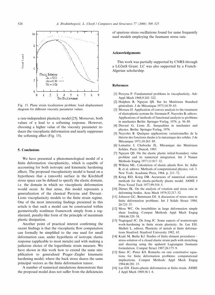
a rate-independent plasticity model [25]. Moreover, both

values of g lead to a softening response. However,

choosing a higher value of the viscosity parameter re-

duces the viscoplastic deformation and nearly suppresses

the softening e�ect (Fig. 15).

5. Conclusions

We have presented a phenomenological model of a

®nite deformation viscoplasticity, which is capable of

accounting for both isotropic and kinematic hardening

e�ects. The proposed viscoplasticity model is based on a

hypotheses that a (smooth) surface in the Kirchho�

stress space can be de®ned to specify the elastic domain,

i.e. the domain in which no viscoplastic deformation

would occur. In that sense, this model represents a

generalization of the classical Perzyna and Duvaut±

Lions viscoplasticity models to the ®nite strain regime.

One of the most interesting ®ndings presented in this

article is that such a model can be constructed within

geometrically nonlinear framework simply from a reg-

ularized, penalty-like form of the principle of maximum

plastic dissipation.

Another point of practical interest con®rming the

recent ®ndings is that the viscoplastic ¯ow computation

can formally be simpli®ed to the one used for small

deformation case, under hypothesis of isotropic elastic

response (applicable to most metals) and with making a

judicious choice of the logarithmic strain measure. We

have shown in this work how to extend the same sim-

pli®cation to generalized Prager±Ziegler kinematic

hardening model, where the back stress shares the same

principal vectors as the ®nite deformation tensor.

A number of numerical simulations demonstrate that

the proposed model does not su�er from the de®ciencies

of spurious stress oscillations found for same frequently

used models employing the Jaumann stress rate.

Acknowledgements

This work was partially supported by CNRS through

a LG2mS Grant. LC was also supported by a French±

Algerian scholarship.

References

[1] Perzyna P. Fundamental problems in viscoplasticity. Adv

Appl Mech 1968;9:243±322.

[2] Halphen B, Nguyen QS. Sur les Mat�eriaux Standard

g�en�eralis�es. J de M�ecanique 1975;14:39±63.

[3] Moreau JJ. Application of convex analysis to the treatment

of elastoplastic systems In: Germain P, Nayroles B, editors.

Applications of methods of functional analysis to problems

in mechanics Berlin: Springer-Verlag, 1976. p. 56±89.

[4] Duvaut G, Lions JL. Inequalities in mechanics and

physics. Berlin: Springer-Verlag, 1976.

[5] Nayroles B. Quelques applications variationnelles de la

th�eorie des fonctions duales �a la m�ecanique des solides. J de

M�ecanique 1971;10:263±89.

[6] Lemaitre J, Chaboche JL. M�ecanique des Mat�eriaux

Solides. Paris: Dunod, 1985.

[7] Nguyen QS. On the elastic plastic initial-boundary value

problem and its numerical integration. Int J Numer

Methods Engng 1977;11:817±32.

[8] Wilkins ML. Calculation of elastic±plastic ¯ow. In: Adler

B, et al. editors. Methods of computational physics, vol. 3.

New York: Academic Press, 1964. p. 211±72.

[9] Krieg RD, Krieg DB. Accuracies of numerical solution

methods for the elastic-perfectly plastic model. ASME J

Press Vessel Tech 1977;99:510±5.

[10] Dienes JK. On the analysis of rotation and stress rate in

deforming bodies. Acta Mech 1979;32:217±32.

[11] Johnson GC, Bammann DJ. A discussion of stress rates in

®nite deformation problems. Int J Solids Struct 1984;

20:725±37.

[12] Moss WC. On instabilities in large deformation simple

shear loading. Comput Methods Appl Mech Engng

1984;46:329±38.

[13] Nagtagaal JC, De Jong JC. Some aspects of nonisotropic

work-hardening in ®nite strain plasticity. In: Lee EH,

Mallett L, editors. Plasticity of metals at ®nite deforma-

tions Stanford: Stanford University 1982, 65.

[14] Koji�c M, Bathe KJ. Studies of ®nite element procedures ±

stress solution of a closed elastic strain path with stretching

and shearing using the updated Lagrangian Jaumann

formulation. Comput Struct 1987;26:175±9.

[15] Simo JC, Pister KS. Remarks on rate constitutive equa-

tions for ®nite deformation problems: computational

implications. Comput Methods Appl Mech Engng

1984;46:201±15.

[16] Lee EH. Elasto-plastic deformation at ®nite strain. ASME

J Appl Mech 1969;36:1±6.

Fig. 15. Plane strain localization problem: load±displacement

diagram for di�erent viscosity parameter values.


[17] Mandel J. Plasticit�e classique et viscoplasticit�e. CISM

courses and lectures 97. Berlin: Springer-Verlag, 1971.

[18] Green AE, Naghdi PM. A general theory of an elasto-

plastic continuum. Arch Rat Mech Anal 1965;18:251±81.

[19] Simo JC, Ortiz M. A uni®ed approach to ®nite deforma-

tion elastoplastic analysis based on the use of hyperelastic

constitutive equations. Comput Mech Appl Mech Engng

1985;49:221±45.

[20] Simo JC. A framework for ®nite strain elastoplasticity

based on maximum plastic dissipation and multiplicative

decomposition. Part I: continuum formulation. Comput

Methods Appl Mech Engng 1988;66:199±219.

[21] Moran B, Ortiz M, Shi CF. Formulation of implicit ®nite

element methods for multiplicative ®nite deformation

plasticity. Int J Numer Methods Engng 1990;29:483±514.

[22] Marsden JE, Hughes TJR. Mathematical foundations of

elasticity. New Jersey: Prentice Hall, 1983.

[23] Ibrahimbegovi�c A. Equivalent Eulerian and Lagrangian

Formulation of Finite Deformation Elastoplasticity in

Principal Axes. Int J Solids Struct 1994;31:3027±40.

[24] Hill R. Aspects of invariance in solid mechanics. Advances

Appl Mech 1978;18:1±75.

[25] Ibrahimbegovi�c A, Gharzeddine F. Finite deformation

plasticity in principal axes: from a manifold to the

euclidean setting. Comput Methods Appl Mech Engng

1998;171:341±69.

[26] Simo JC. Algorithms for static and dynamic multiplicative

plasticity that preserve the classical return mapping

schemes of the in®nitesimal theory. Comput Methods

Appl Mech Engng 1992;99:61±112.

[27] Weber G, Anand L. Finite deformation constitutive

equations and a time integration procedure for isotropic,

hyperelastic-viscoplastic solids. Comput Methods Appl

Mech Engng 1990;79:173±202.

[28] Peri�c D, Owen DRJ, Honnor ME. A model for ®nite strain

elasto-plasticity based on logarithmic strains: computa-

tional issues. Comput Methods Appl Mech Engng 1992;

94:35±61.

[29] Eterovic AL, Bathe KJ. A hyperelastic-based large strain

elasto-plastic constitutive formulation with combined iso-

tropic-kinematic hardening using the logarithmic stress

and strain measures. Int J Numer Methods Engng 1990;

30:1099±114.

[30] Cuitino A, Ortiz M. A material-independent method for

extending stress update algorithms from small-strain plas-

ticity to ®nite plasticity with multiplicative kinematics.

Engng Comput 1992;9:437±51.

[31] Naghdi PM. A critical review of the state of ®nite

plasticity. J Appl Math Phys (ZAMP) 1990;41:315±94.

[32] Gurtin ME. An introduction to continuum mechanics.

New York: Academic Press, 1981.

[33] Coleman BD, Gurtin ME. Thermodynamics with internal

variables. J Chem Phys 1967;47:597±613.

[34] Germain P, Nguyen QS, Suquet P. Continuum thermody-

namics. ASME J Appl Mech 1983;50:1010±20.

[35] Maugin G. The thermomechanics of plasticity and frac-

ture. Cambridge: Cambridge University Press, 1992.

[36] Hill R. The mathematical theory of plasticity. London:

Oxford University Press, 1950.

[37] Lubliner J. A maximum-dissipation principle in general-

ized plasticity. Acta Mech 1984;52:225±37.

[38] Germain P. Duality and convection in continuum me-

chanics. In: Fichera G, et al. editors. Trends in Applica-

tions of Pure Mathematics to Mechanics, Pitman: London,

1976, pp.107±28.

[39] Zienkiewicz OC, Taylor RL. The ®nite element method:

basic formulation and linear problems. London: McGraw-

Hill, 1989.

[40] Bathe JK. Finite element procedures. New Jersey: Prentice

Hall, 1996.

[41] Ibrahimbegovi�c A, Gharzeddine F, Chor® L. Classical

plasticity and viscoplasticity models reformulated: theoret-

ical basis and numerical implementation. Int J Numer

Methods Engng 1998;42:1499±535.

[42] Ibrahimbegovi�c A. Finite elastoplastic deformations of

space-curved membranes. Comput Methods Appl Mech

Engng 1994;119:371±94.

[43] Dafailas YF. Corotational rates for kinematic hardening

at large plastic deformations. ASME J Appl Mech

1983;50:561±5.

[44] Tvergaard V, Needleman A, Lo KK. Flow localization in

the plane strain tensile test. J Mech Phys Solids 1981;

29:115±42.

[45] Needleman A. Material rate dependence and mesh sensi-

tivity in localization problems. Comput Methods Appl

Mech Engng 1988;67:69±85.


Documents

10.1.1.103.7728