10.02.08 1WSC-6

Critical levels in projectionCritical levels in projection

Alexey PomerantsevSemenov Institute of Chemical Physics, Moscow

10.02.08 2WSC-6

Projection approachProjection approach

10.02.08 3WSC-6

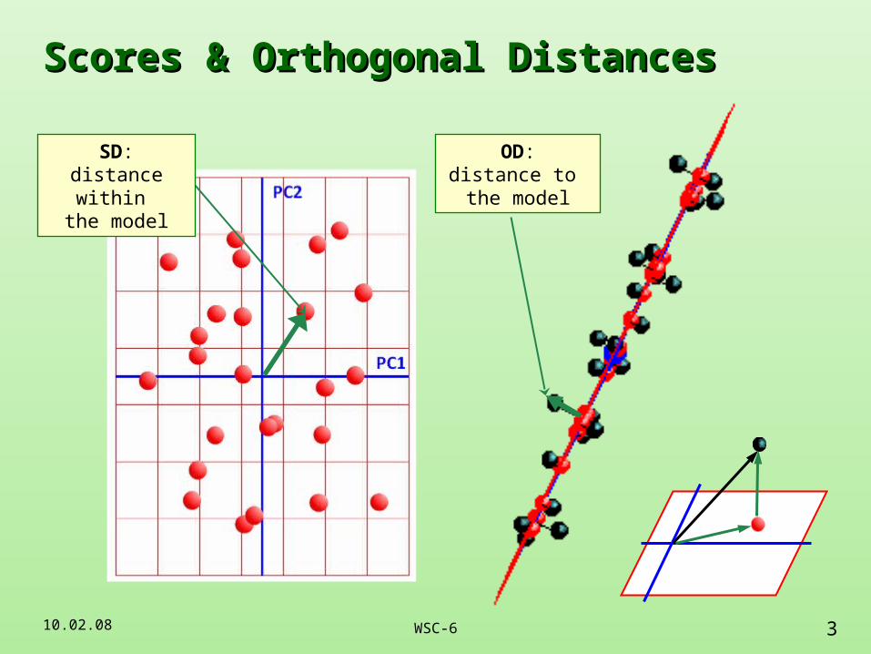
Scores & Orthogonal DistancesScores & Orthogonal Distances

OD:distance to the model

SD:distance within

the model

10.02.08 4WSC-6

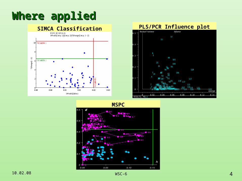
Where appliedWhere applied

0

2

4

6

8

10

0.00 0.00 0.01 0.01 0.02 0.03

T2R

ange

[1 -

2]

DModX[2](Abs)

MSPC.M3 (PCA-X)DModX[Comp. 2][Comp. 2]/T2Range[Comp. 1 - 2]

M3-D-Crit[2] = 0.01992 T2Crit(95%) = 6.48227 T2Crit(99%) = 10.2923

D-C

rit(0

.05)

T2Crit(95%)

T2Crit(99%)

SIMCA-P+ 11.5 - 20.01.2008 17:30:53

SIMCA Classification

0

0.1

0.2

0.3

0.4

0.5

0 0.02 0.04 0.06 0.08 0.10 0.12 0.14 RESULT2, PC: 4,4

1

23

4

5

6

7

8

9

10

1112131415161718

1920

21222324

25

26272829

3031

32

33

3435

36

37

383940414243

44

45

4647

48

4950

51

52

53

54

55

56

57

5859

60

61

62

63646566

67

6869

70

71

7273

74

75

76

777879

80

81

82

83

84

85

86

878889

90

91929394

95

96

97

9899100101102

103

104

105

106107

108

109

110

111112

113

114

115116

117

118119

120

121122 123

Leverage

Residual Y-variance Influence

PLS/PCR Influence plot

t69t68 t67

t66t65t64

t63

t62

t61 t60t59

t58t57t56t55

t54t53

t52t51t50 t49

t48t47

t46t45t44t43

t42

t41t40

t39t38

t37t36

t35

t34

t33

t32t31

t30t29

t28t27

t26t25

t24t23

t22t21

t20t19

t18t17

t16t15

t14t13t12t11

t10t9

t8t7

t6t5 t4

t3

t2

t10

0.1

0.2

0.3

0.4

0.5

0.00 0.05 0.10 0.15

h

dMSPC

10.02.08 5WSC-6

Giants battle at ICS-L, April 2007Giants battle at ICS-L, April 2007

The ratios of residual variances of PCA are fairly

well F-distributed. This is easy - the shape of the

distribution of a ratio of two variances usually

looks like an F.Svante Wold

No, the residuals from PCA don't follow an F-

distribution unless you fuss with the degrees of

freedom, and there are better alternatives in any

case.Barry Wise

10.02.08 6WSC-6

Full PCA DecompositionFull PCA Decomposition

K=rank(X) ≤ min (I, J)

X=TPt =TtT=diag(1,.., K)

I

iikk t

1

2

K

kkL

1

tt0 )Sp()Sp( TTXX

XI

J K

TI= ×Pt

J

K

10.02.08 7WSC-6

Truncated PCA DecompositionTruncated PCA Decomposition

AAA EPTX t

0

1

)( LARA

aa

A ≤ K

I

A

TA

A PA

EA+X I= × J

J

t

I

J

10.02.08 8WSC-6

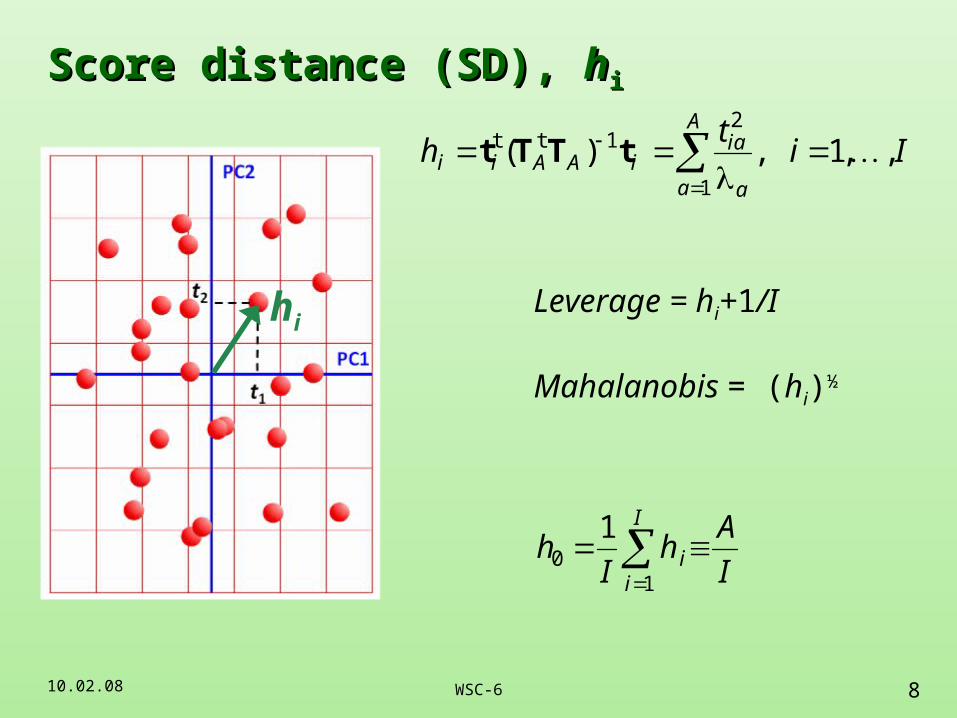
Score distance (SD), Score distance (SD), hhii

Iit

hA

a a

iaiAAii ,,1,)(

1

21tt

tTTt

I

ii I

Ah

Ih

10

1

hi Leverage = hi+1/I

Mahalanobis = (hi)½

10.02.08 9WSC-6

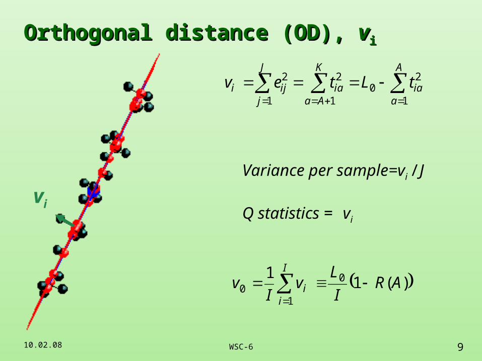
Orthogonal distance (OD), Orthogonal distance (OD), vvii

I

ii AR

I

Lv

Iv

1

00 )(1

1

vi

A

aia

K

Aaia

J

jiji tLtev

1

20

1

2

1

2

Variance per sample=vi /J

Q statistics = vi

10.02.08 10WSC-6

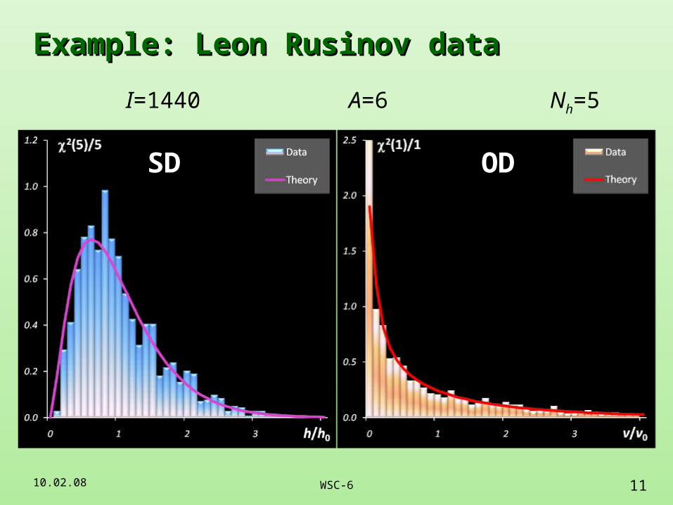
Distribution of distances: the shape?Distribution of distances: the shape?

=h/h0x= =v/v0

x ~ χ2(N)/N

N = DoF

E(x) = 1

D(x) = 2/N

10.02.08 11WSC-6

Example: Leon Rusinov dataExample: Leon Rusinov data

I=1440 A=6 Nh=5 Nv=1

SD OD

10.02.08 12WSC-6

Distribution of distances: DoF?Distribution of distances: DoF?

Method of Moments

I

iix

IS

1

22 )1(1

2

2ˆS

N

Interquartile Approach

x(1) ≤ x(2 )≤ .... ≤ x(I-1) ≤ x(I)

¼ IQR ¼

IQR

N

NN

)41,()43,( 22

= h/h0x= = v/v0

x1,...., xI ~ χ2(N)/N N = ?

10.02.08 13WSC-6

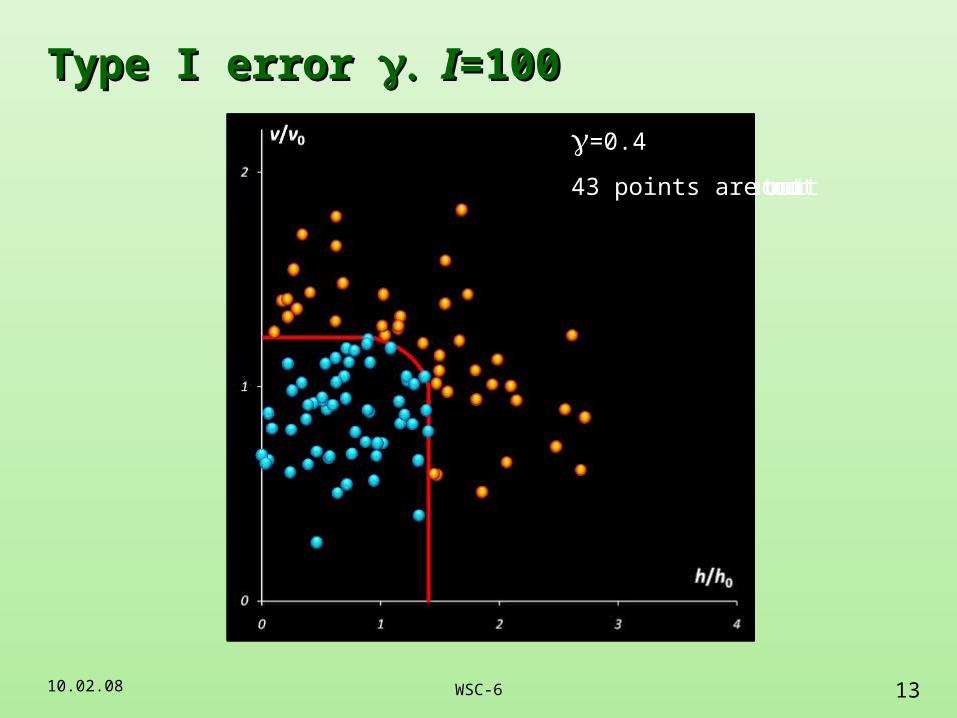
Type I error Type I error II=100=100

=0.01

1 point is out

=0.05

5 points are out

=0.1

11 points are out

=0.2

22 points are out

=0.4

43 points are out

10.02.08 14WSC-6

SIM Data. MSPC taskSIM Data. MSPC task

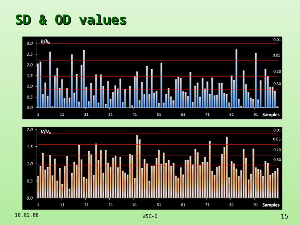
I=100 J=25 A=5 =0.05

sim

t55 EPTX

10.02.08 15WSC-6

SD & OD valuesSD & OD values

10.02.08 16WSC-6

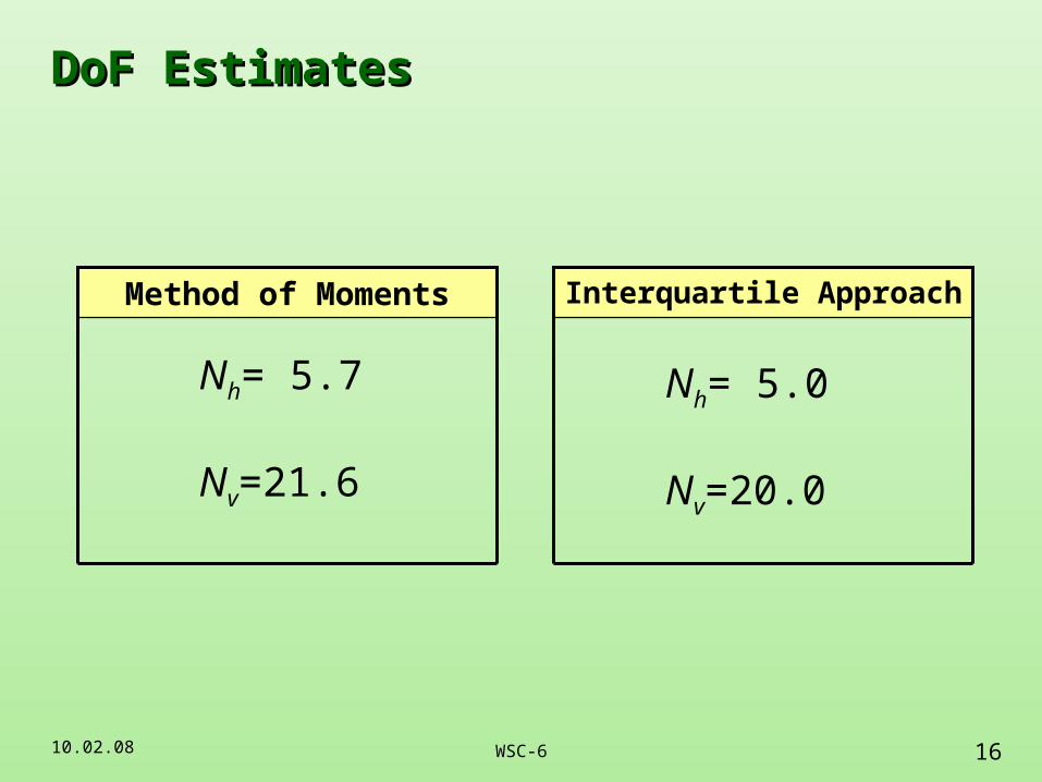
DoF EstimatesDoF Estimates

Interquartile ApproachMethod of Moments

Nh= 5.7 Nv=21.6

Nh= 5.0 Nv=20.0

10.02.08 17WSC-6

Acceptance areas: conventionalAcceptance areas: conventional

11

),(,0

),(,0

20

20

vv

hh

NN

v

NN

hH

I=100 =0.05

10.02.08 18WSC-6

Acceptance areas Acceptance areas =0.05: Sum of CHIs=0.05: Sum of CHIs

)(~ 2

00vhvh NN

v

vN

h

hN

I=100 =0.05

10.02.08 19WSC-6

Acceptance areas: Ratio of CHIsAcceptance areas: Ratio of CHIs

),(F~

0

0hv NN

hh

vv

I=100 =0.05

10.02.08 20WSC-6

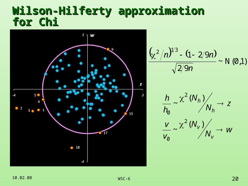
Wilson-Hilferty approximation for Chi Wilson-Hilferty approximation for Chi

wNN

v

v

zNN

h

h

v

v

h

h

)(~

)(~

2

0

2

0

)1,0(N~

92

921312

n

nn

10.02.08 21WSC-6

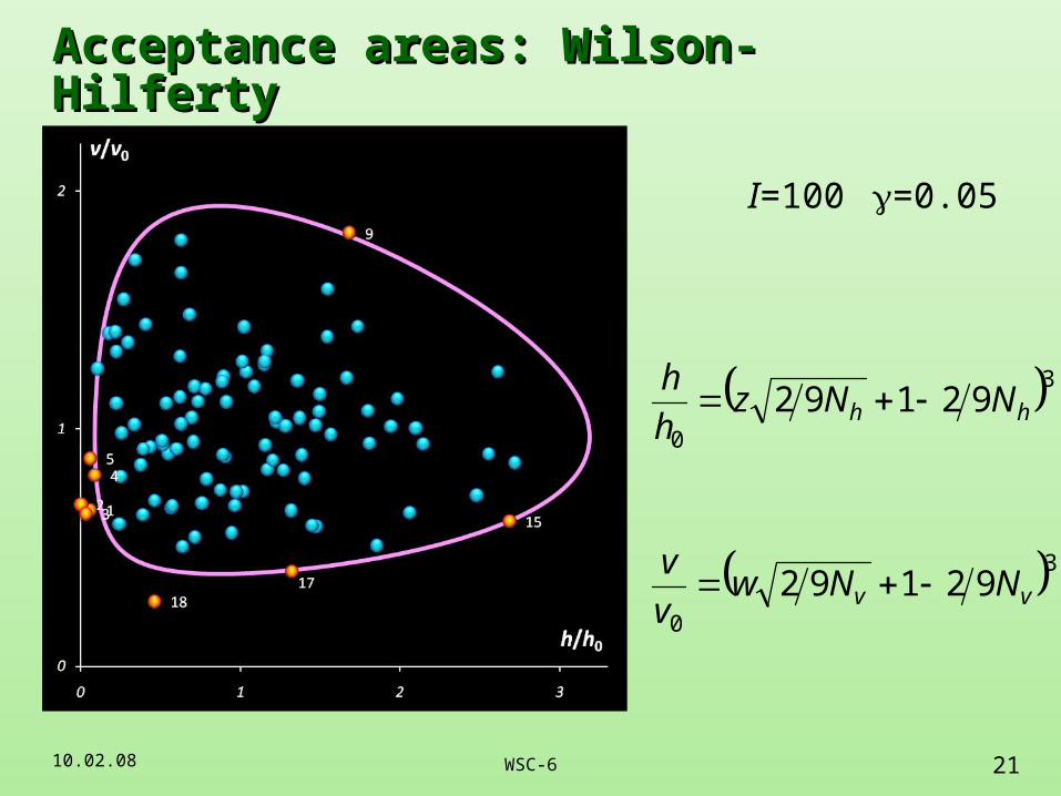
Acceptance areas: Wilson-HilfertyAcceptance areas: Wilson-Hilferty

30

92192 hh NNzh

h

30

92192 vv NNwv

v

I=100 =0.05

10.02.08 22WSC-6

Modified Wilson-Hilferty approximationModified Wilson-Hilferty approximation

1–γ=P0+P1+P2+P3=

= Φ(r) – ¼exp(–½r2)

r=r(γ)

10.02.08 23WSC-6

Acceptance areas: modified Wilson-HilfertyAcceptance areas: modified Wilson-Hilferty

30

92192 hh NNzh

h

30

92192 vv NNwv

v

I=100 =0.05

10.02.08 24WSC-6

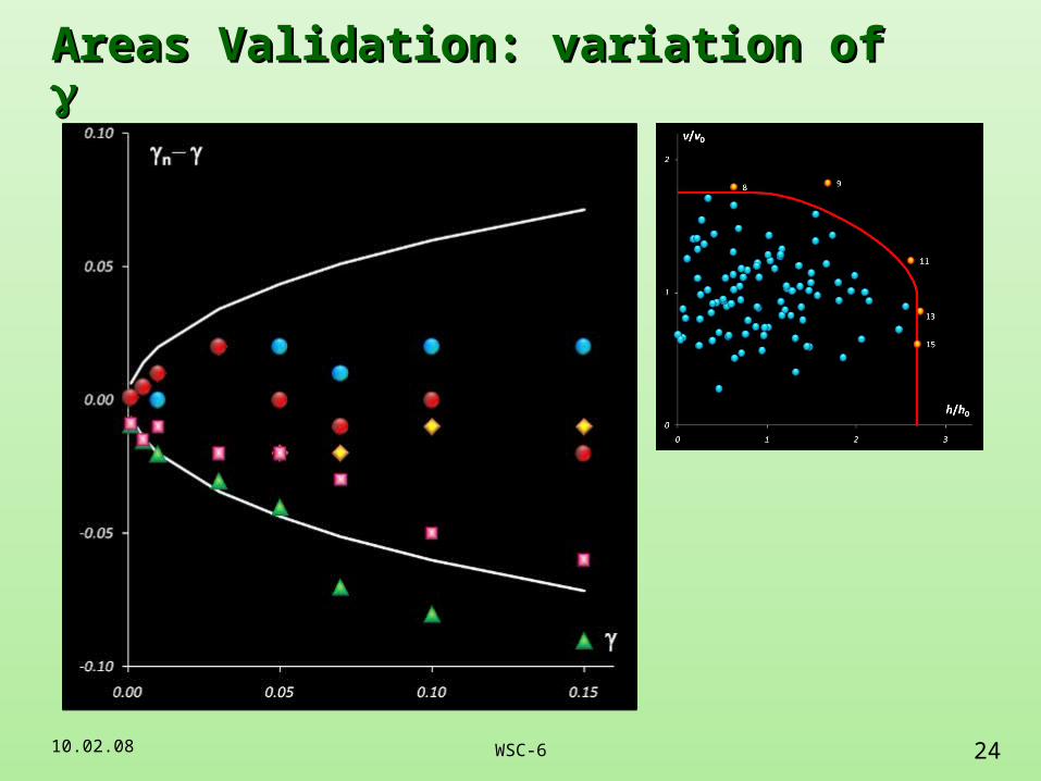
Areas Validation: variation of Areas Validation: variation of

10.02.08 25WSC-6

BMT Data. SIMCABMT Data. SIMCA I=45 J=3501 A=2

Nh=3 Nv=2 =0.025

10.02.08 26WSC-6

Extremes & Outliers in calibration setExtremes & Outliers in calibration set

is significance

level for outliers

=1 – (1 – )1/I

extreme

outlier

Calibration set: I=45

γ I = 0.02545 = 1.25

Iout=2

10.02.08 27WSC-6

SIMCA Classification without G07-4 SIMCA Classification without G07-4

New set: Inew=30

10 Genuine + 20 Fakes

γ I new= 0.02510 = 0.25

Iout=3

10.02.08 28WSC-6

What’s up?What’s up?

This is absolutely wrong classification but Oxana will

explain how fix it over.

10.02.08 29WSC-6

GRAIN Data. Influence plotsGRAIN Data. Influence plots

I=123 J=118 A=4 =0.01

Nh=5.7 Nv=3.0 Nu=1.0

8 10 12 14

X Y

10.02.08 30WSC-6

Orthogonal distance to YOrthogonal distance to Y

)1()ˆ( 2iiii hyyu

10.02.08 31WSC-6

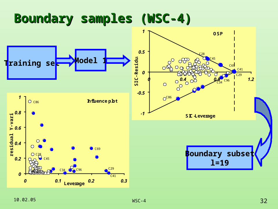
Back to WSC-4Back to WSC-4

10.02.05 32WSC-4

Training set Model 1

Boundary subsetl=19

Influence plot

C45

C34

C41

C29

C69

C28

C96

C86

0

0.2

0.4

0.6

0.8

1

0 0.1 0.2 0.3Leverage

res

idu

al Y

-va

ria

nc

e

Boundary samples (WSC-4)Boundary samples (WSC-4)OSP

C34

C41C69

C45

C86

C96

C29

C28

-1

-0.5

0

0.5

1

0 0.4 0.8 1.2

SIC-Leverage

SIC

-Re

sid

ua

l

`

10.02.08 33WSC-6

Influence plots for X and YInfluence plots for X and Y

YX

Calibration Boundary (SIC)

10.02.08 34WSC-6

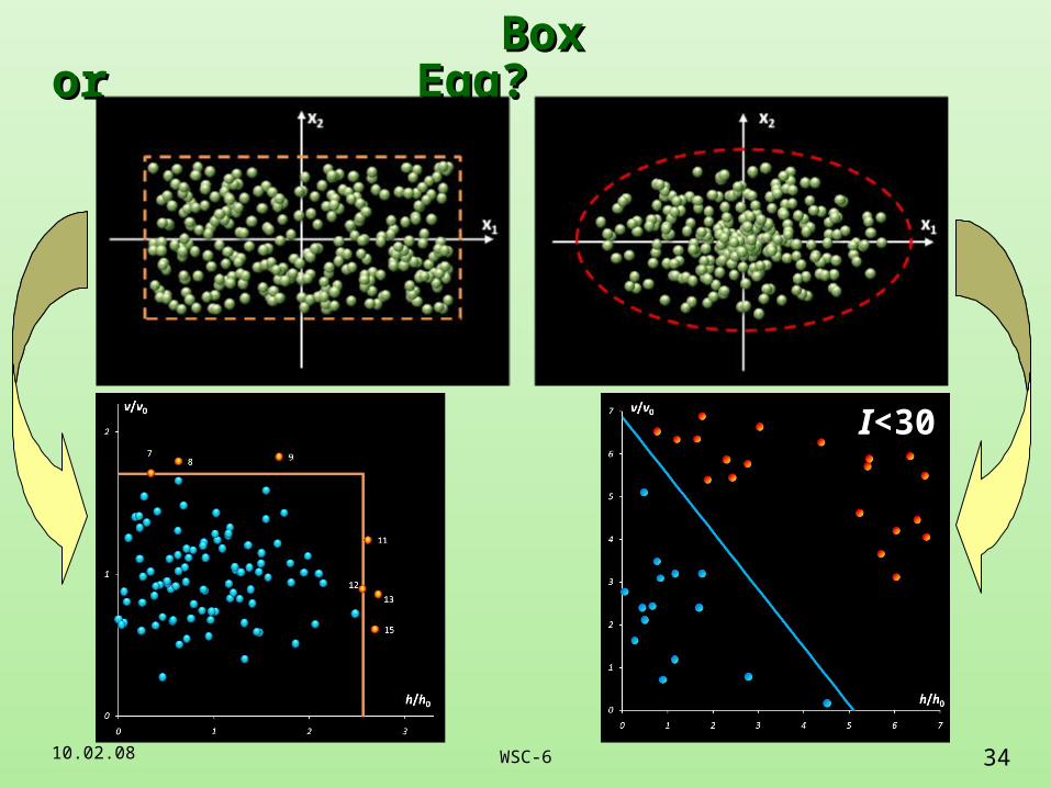
Box or Egg?Box or Egg?

I<30

10.02.08 35WSC-6

Conclusion 1Conclusion 1

The χ2-distribution can be used in the modeling of the score

and orthogonal distances.

10.02.08 36WSC-6

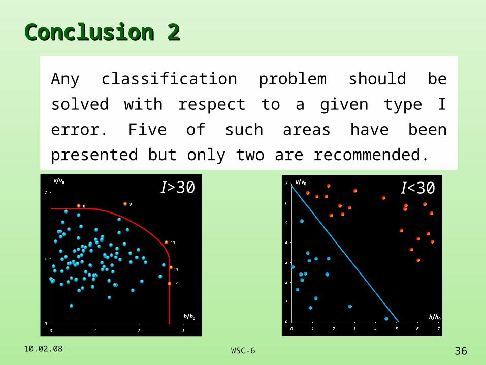
Conclusion 2Conclusion 2

Any classification problem should be solved with respect to

a given type I error. Five of such areas have been presented

but only two are recommended.

I>30 I<30

10.02.08 37WSC-6

Conclusion 3Conclusion 3

Estimation of DoF is a key challenge in the projection

modeling. A data-driven estimator of DoF, rather than a

theory-driven one should be used. The method of moments

is effective, but sensitive to outliers. The IQR estimator is a

robust but less effective alternative.

More examples will be demonstrated in the subsequent

presentation by Oxana.