Embed Size (px)
Citation preview
10.02.05 1WSC-4
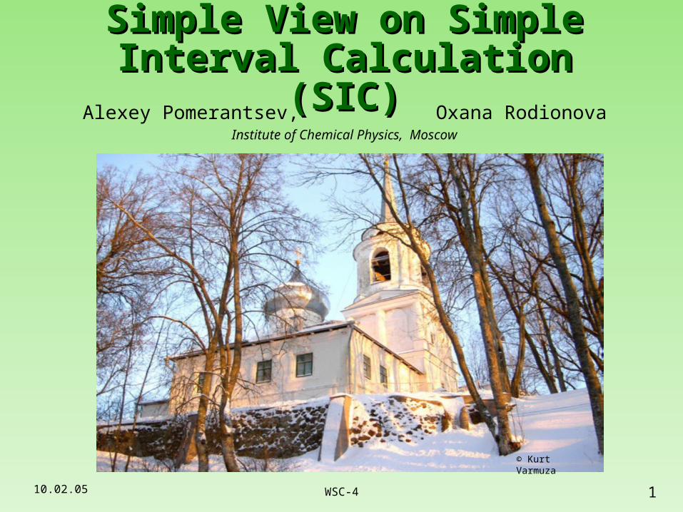
Simple View on Simple Interval Simple View on Simple Interval Calculation (SIC)Calculation (SIC)
Alexey Pomerantsev, Oxana RodionovaInstitute of Chemical Physics, Moscow
and Kurt VarmuzaVienna Technical University
© Kurt Varmuza
10.02.05 2WSC-4
CAC, Lisbon, September 2004CAC, Lisbon, September 2004
10.02.05 3WSC-4
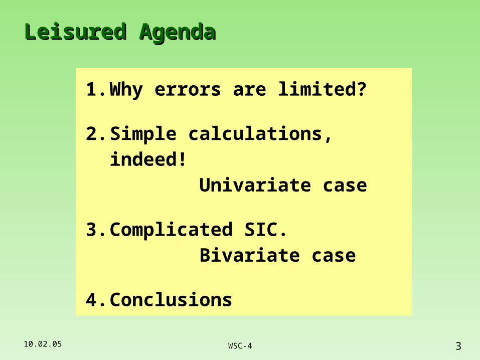
Leisured AgendaLeisured Agenda
1. Why errors are limited?
2. Simple calculations, indeed! Univariate case
3. Complicated SIC. Bivariate case
4. Conclusions
10.02.05 4WSC-4
Part I. Why errors are limited?Part I. Why errors are limited?
10.02.05 5WSC-4
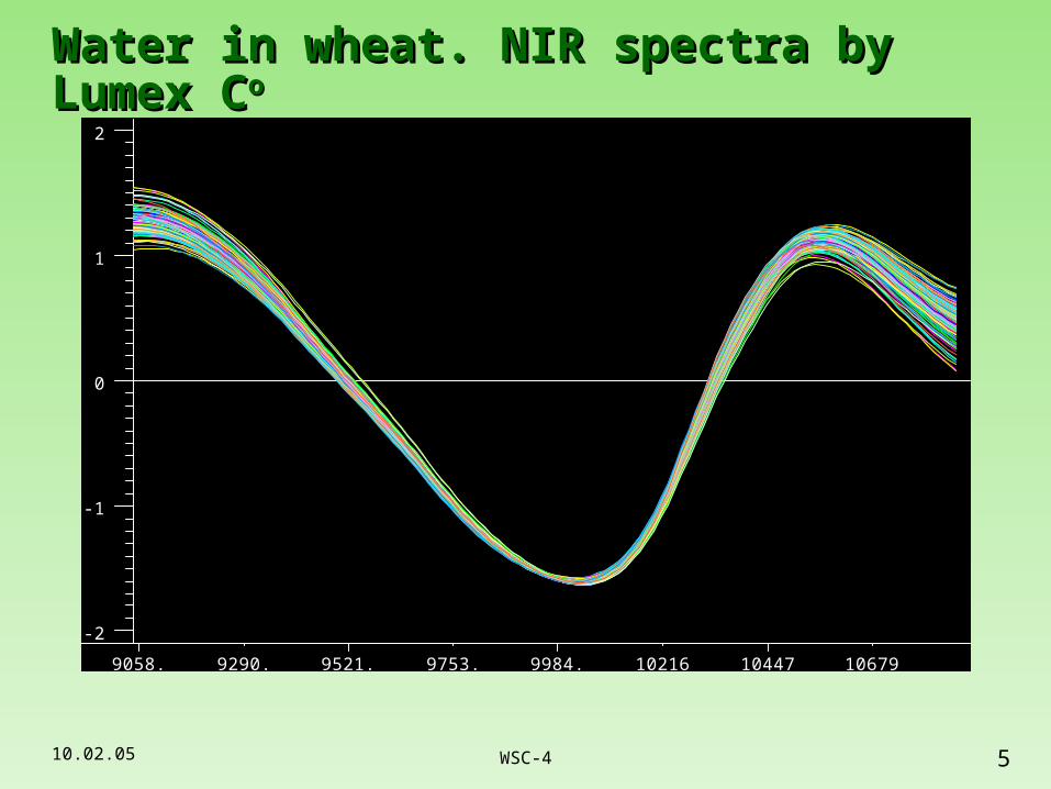
Water in wheat. NIR spectra by Lumex CWater in wheat. NIR spectra by Lumex Coo
-2
-1
0
1
2
9058. 9290. 9521. 9753. 9984. 10216 10447 10679
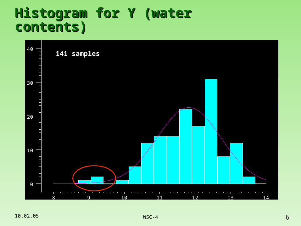
10.02.05 6WSC-4
Histogram for Y (water contents)Histogram for Y (water contents)
0
10
20
30
40
8 9 10 11 12 13 14
141 samples
10.02.05 7WSC-4
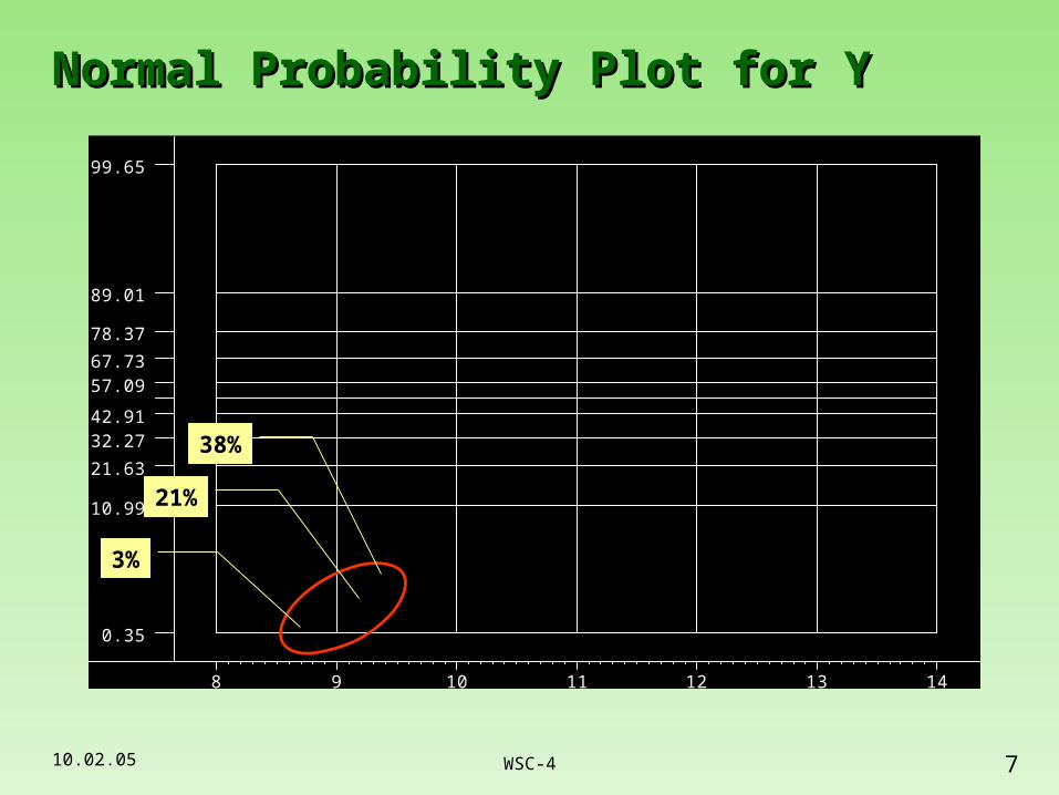
Normal Probability Plot for YNormal Probability Plot for Y
0.35
10.99
21.63
32.27 42.91
99.65
89.01
78.37
67.73 57.09
8 9 10 11 12 13 14
3%
21%
38%
10.02.05 8WSC-4
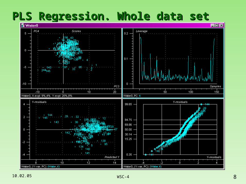
PLS Regression. Whole data setPLS Regression. Whole data set
10.02.05 9WSC-4
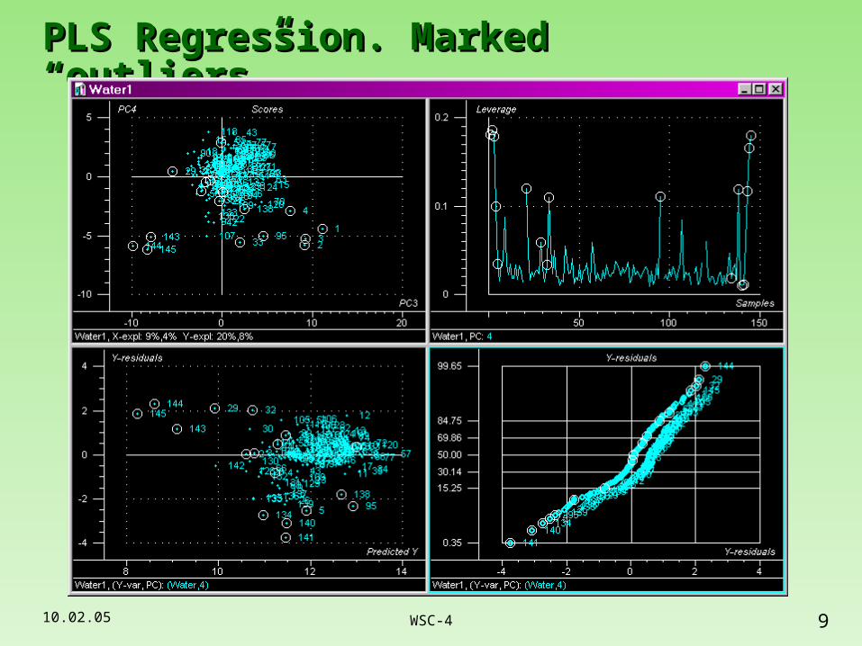
PLS Regression. Marked “outliers”PLS Regression. Marked “outliers”
10.02.05 10WSC-4
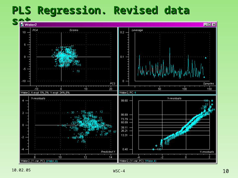
PLS Regression. Revised data setPLS Regression. Revised data set
10.02.05 11WSC-4
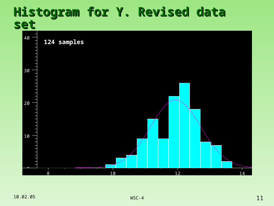
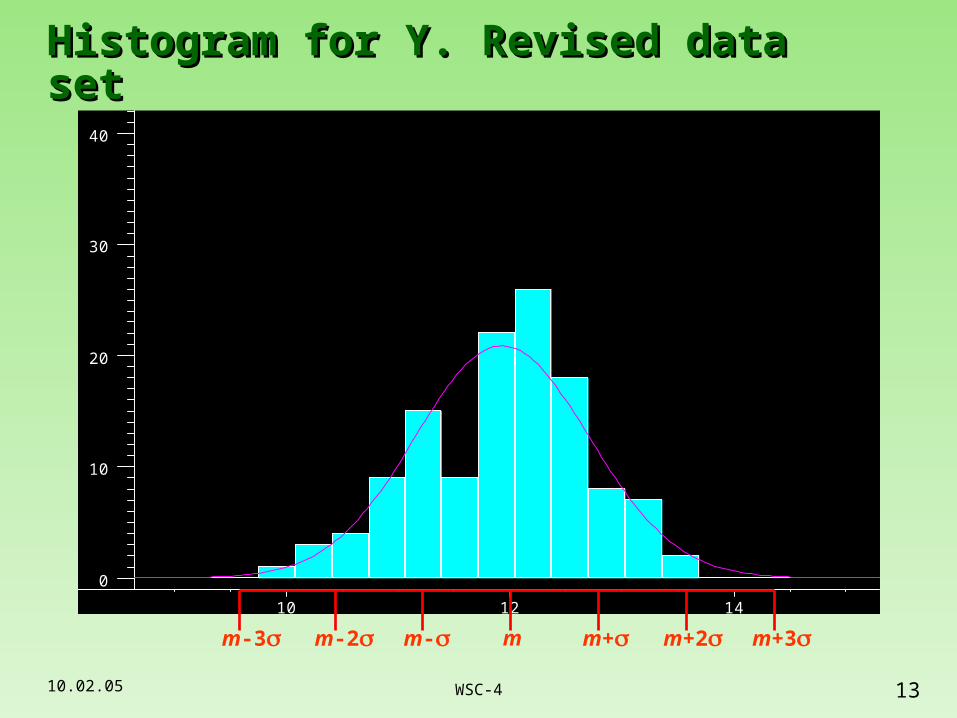
Histogram for Y. Revised data setHistogram for Y. Revised data set
0
10
20
30
40
8 10 12 14
124 samples
10.02.05 12WSC-4
0.40
10.08
19.76
29.44 39.11
99.60
89.92
80.24
70.56 60.89
9 10 11 12 13 14
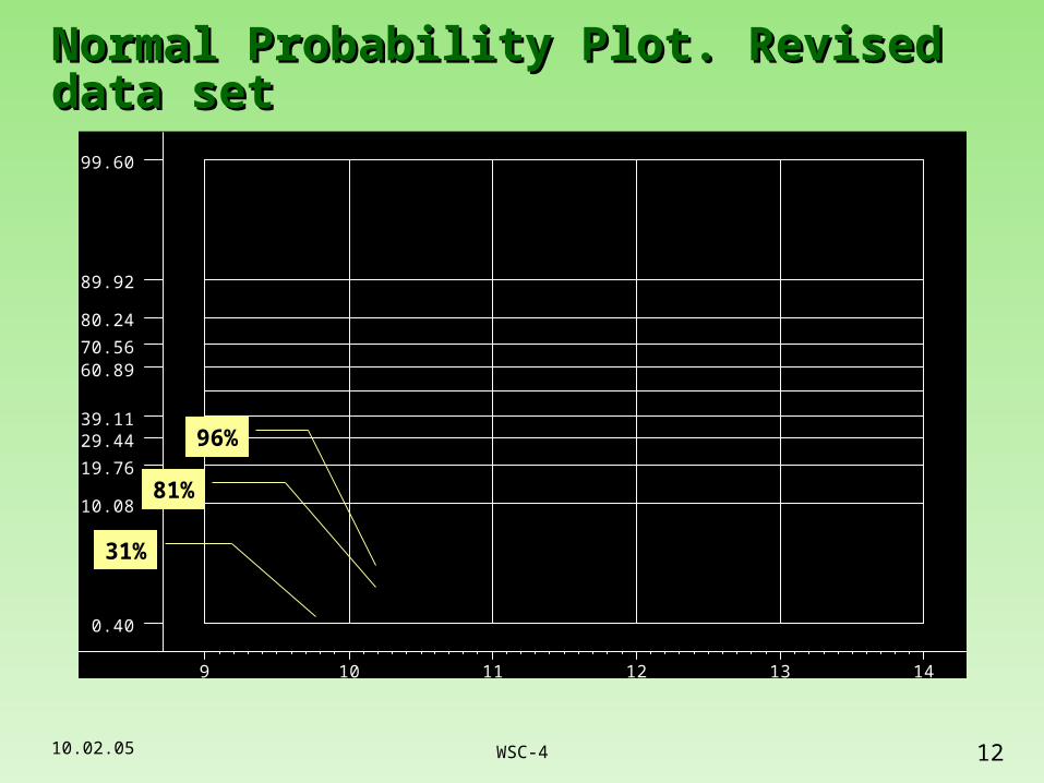
Normal Probability Plot. Revised data Normal Probability Plot. Revised data setset
31%
81%
96%
10.02.05 13WSC-4
0
10
20
30
40
10 12 14
Histogram for Y. Revised data setHistogram for Y. Revised data set
m+ m+2 m+3m-3 m-2 m- m
10.02.05 14WSC-4
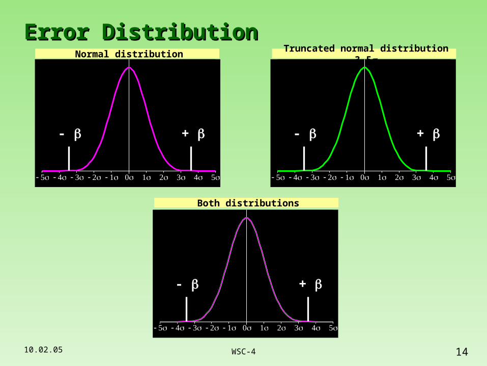
Error DistributionError Distribution
+ -
Normal distribution Truncated normal distribution 3.5
+ -
Both distributions
+ -
10.02.05 15WSC-4
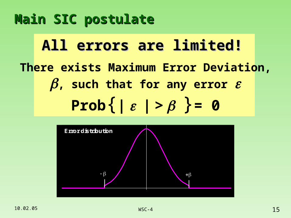
Main SIC postulateMain SIC postulate
All errors are limited!All errors are limited!
There exists Maximum Error Deviation,
, such that for any error Prob{| | > }= 0
Error distribution
10.02.05 16WSC-4
Part 2. Simple calculationsPart 2. Simple calculations
10.02.05 17WSC-4
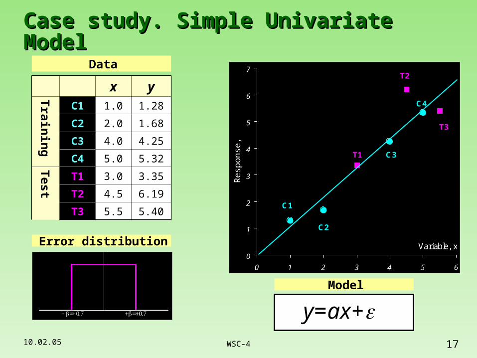
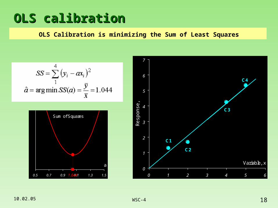
Case study. Simple Univariate ModelCase study. Simple Univariate Model
x y
Train
ing
C1 1.0 1.28
C2 2.0 1.68
C3 4.0 4.25
C4 5.0 5.32
Test
T1 3.0 3.35
T2 4.5 6.19
T3 5.5 5.40
Data
C4
C3
C2
C1
T2
T3
T1
0
1
2
3
4
5
6
7
0 1 2 3 4 5 6
Variable, xR
espo
nse,
y
y=ax+Model
Error distribution
10.02.05 18WSC-4
OLS calibrationOLS calibrationOLS Calibration is minimizing the Sum of Least Squares
C4
C3
C2
C1
T2
T3
T1
0
1
2
3
4
5
6
7
0 1 2 3 4 5 6
Variable, x
Res
pons
e, y
Sum of Squares
0.70.5 0.7 0.9 1.1 1.3 1.5
a
Sum of Squares
1.40.5 0.7 0.9 1.1 1.3 1.5
a
C4
C3
C2
C1
T2
T3
T1
0
1
2
3
4
5
6
7
0 1 2 3 4 5 6
Variable, x
Res
pons
e, y
Sum of Squares
0.80.5 0.7 0.9 1.1 1.3 1.5
a
C4
C3
C2
C1
T2
T3
T1
0
1
2
3
4
5
6
7
0 1 2 3 4 5 6
Variable, x
Res
pons
e, y
Sum of Squares
1.20.5 0.7 0.9 1.1 1.3 1.5
a
C4
C3
C2
C1
T2
T3
T1
0
1
2
3
4
5
6
7
0 1 2 3 4 5 6
Variable, x
Res
pons
e, y
Sum of Squares
1.0440.5 0.7 0.9 1.1 1.3 1.5
a
C4
C3
C2
C1
T2
T3
T1
0
1
2
3
4
5
6
7
0 1 2 3 4 5 6
Variable, x
Res
pons
e, y
10.02.05 19WSC-4
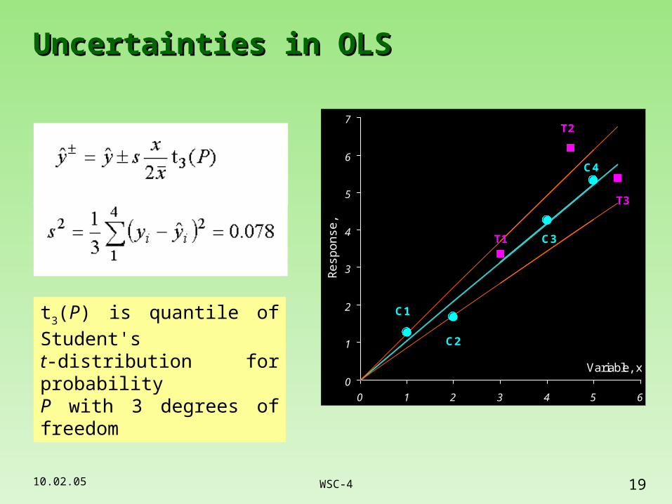
Uncertainties in OLSUncertainties in OLS
t3(P) is quantile of Student's
t-distribution for probabilityP with 3 degrees of freedom
C1
C2
C3
C4
T1
T3
T2
0
1
2
3
4
5
6
7
0 1 2 3 4 5 6
Variable, x
Res
pons
e, y
10.02.05 20WSC-4
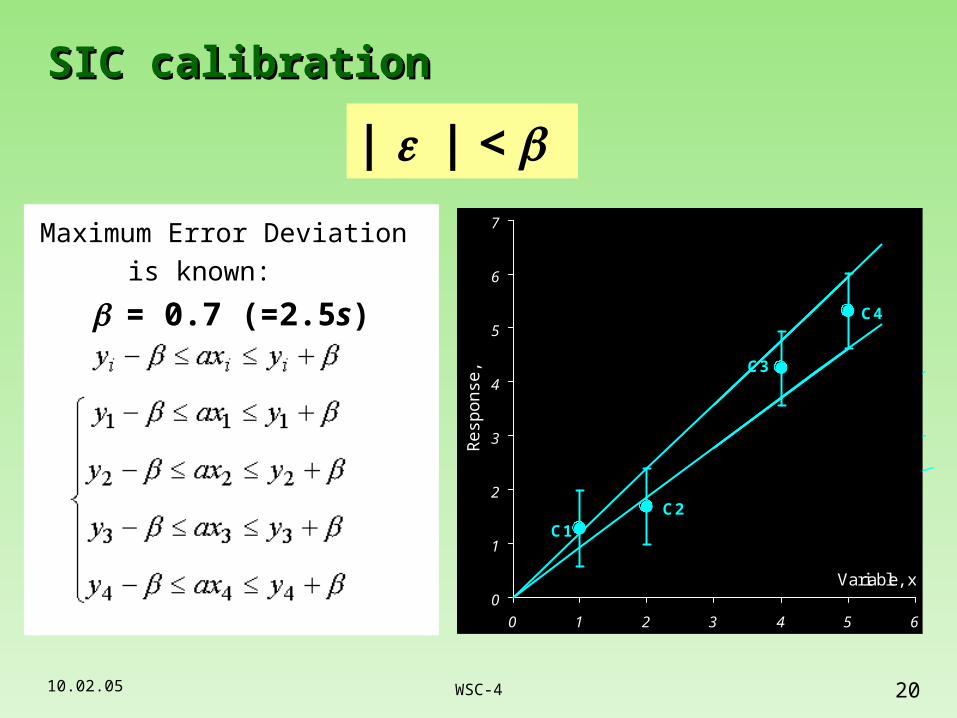
Maximum Error Deviation
is known:
= 0.7 (=2.5s)
SIC calibrationSIC calibration
C4
C3
C2C1
0
1
2
3
4
5
6
7
0 1 2 3 4 5 6
Variable, x
Res
pons
e, y
C4
C3
C2C1
0
1
2
3
4
5
6
7
0 1 2 3 4 5 6
Variable, x
Res
pons
e, y
22
2
2C4
C3
C2C1
0
1
2
3
4
5
6
7
0 1 2 3 4 5 6
Variable, x
Res
pons
e, y
| | <
10.02.05 21WSC-4
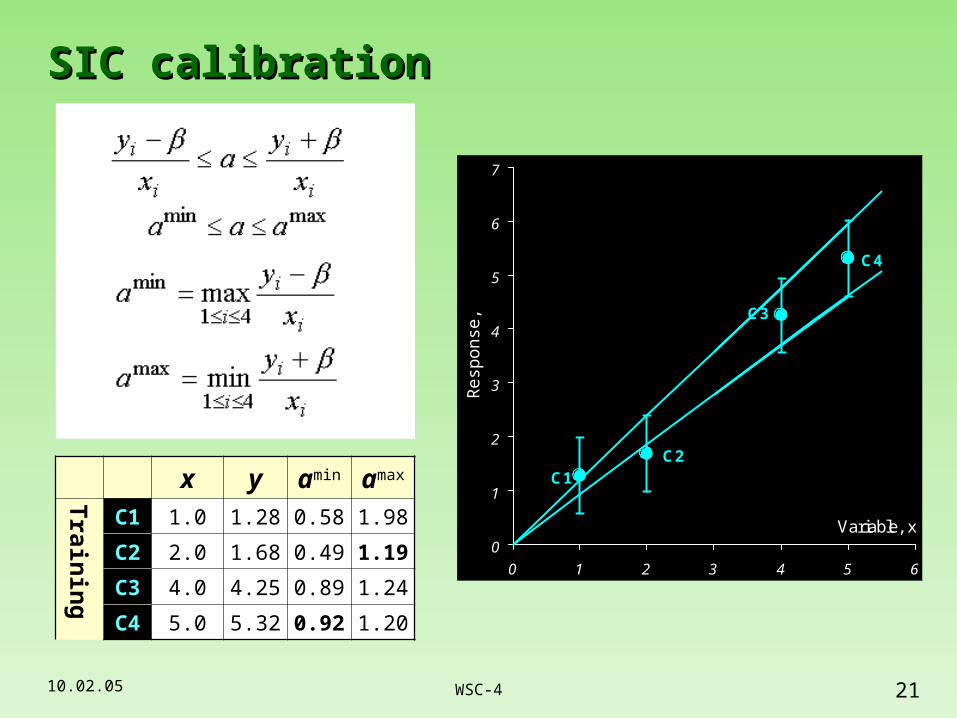
SIC calibrationSIC calibration
x y amin amax
Train
ing
C1 1.0 1.28 0.58 1.98
C2 2.0 1.68 0.49 1.19
C3 4.0 4.25 0.89 1.24
C4 5.0 5.32 0.92 1.20
C4
C3
C2C1
0
1
2
3
4
5
6
7
0 1 2 3 4 5 6
Variable, x
Res
pons
e, y
10.02.05 22WSC-4
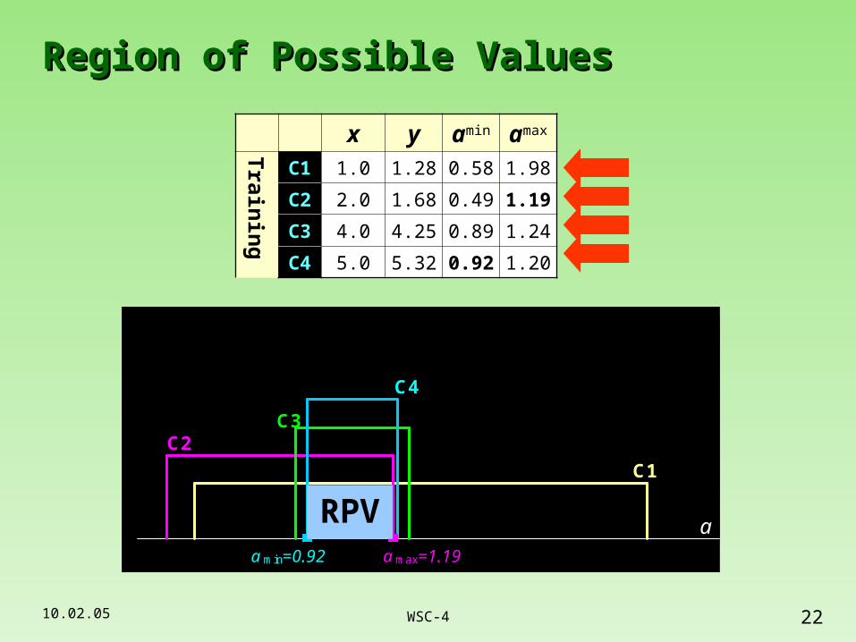
Region of Possible ValuesRegion of Possible Values
x y amin amax
Train
ing
C1 1.0 1.28 0.58 1.98
C2 2.0 1.68 0.49 1.19
C3 4.0 4.25 0.89 1.24
C4 5.0 5.32 0.92 1.20
C1
a
C1
C2
a
C1
C2C3
a
C1
C2C3
C4
a
C1
C2
a max=1.19
C3
C4
a min=0.92
aRPV
10.02.05 23WSC-4
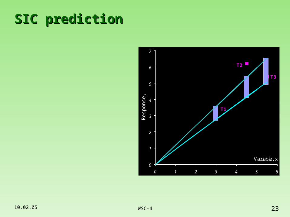
SIC predictionSIC prediction
C4
C3
C2C1
0
1
2
3
4
5
6
7
0 1 2 3 4 5 6
Variable, x
Res
pons
e, y
T2
T3
T1
0
1
2
3
4
5
6
7
0 1 2 3 4 5 6
Variable, x
Res
pons
e, y
T1
T3
T2
0
1
2
3
4
5
6
7
0 1 2 3 4 5 6
Variable, x
Res
pons
e, y
x y v - v +
Test
T1 3.0 3.35 2.77 3.57
T2 4.5 6.19 4.16 5.36
T3 5.5 5.40 5.08 6.55
10.02.05 24WSC-4
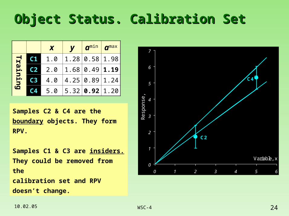
Object Status. Calibration SetObject Status. Calibration Set
C4
C3
C2C1
0
1
2
3
4
5
6
7
0 1 2 3 4 5 6
Variable, x
Res
pons
e, y
C2
C4
0
1
2
3
4
5
6
7
0 1 2 3 4 5 6
Variable, x
Res
pons
e, y
x y amin amax
Train
ing
C1 1.0 1.28 0.58 1.98
C2 2.0 1.68 0.49 1.19
C3 4.0 4.25 0.89 1.24
C4 5.0 5.32 0.92 1.20
Samples C2 & C4 are the boundary
objects. They form RPV.
Samples C1 & C3 are insiders.
They could be removed from the
calibration set and RPV doesn’t
change.
10.02.05 25WSC-4
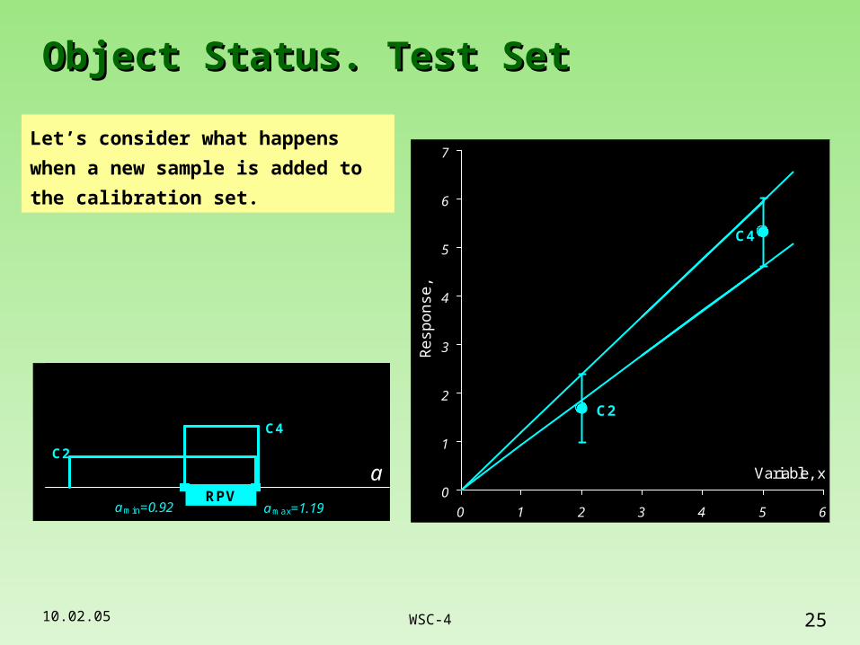
Object Status. Test SetObject Status. Test Set
C2
C4
0
1
2
3
4
5
6
7
0 1 2 3 4 5 6
Variable, x
Res
pons
e, y
Let’s consider what happens when a
new sample is added to the calibration
set.
amax=1.19
C2
amin=0.92
C4
aRPV
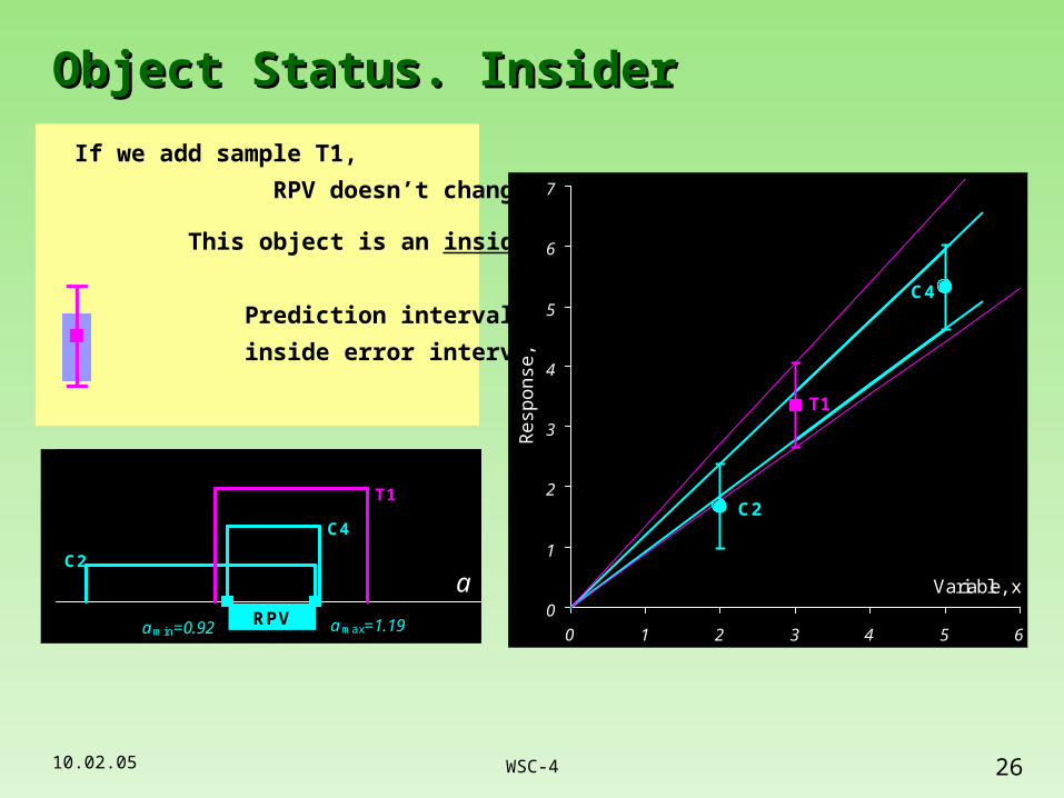
10.02.05 26WSC-4
Object Status. InsiderObject Status. Insider
If we add sample T1,
RPV doesn’t change.
This object is an insider.
Prediction interval lies
inside error interval
C4
C2
T1
0
1
2
3
4
5
6
7
0 1 2 3 4 5 6
Variable, x
Res
pons
e, y
C2
amax=1.19
C4
amin=0.92
T1
aRPV
10.02.05 27WSC-4
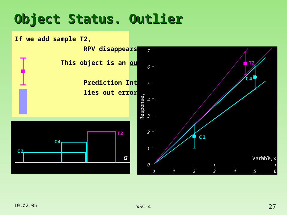
Object Status. OutlierObject Status. Outlier
If we add sample T2,
RPV disappears.
This object is an outlier.
Prediction Interval
lies out error interval
C2
C4
T2
0
1
2
3
4
5
6
7
0 1 2 3 4 5 6
Variable, x
Res
pons
e, y
amax=1.19
C2
amin=0.92
C4
T2
a
10.02.05 28WSC-4
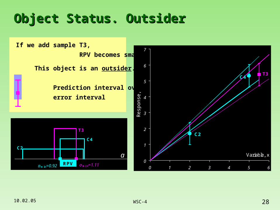
Object Status. OutsiderObject Status. Outsider
If we add sample T3,
RPV becomes smaller.
This object is an outsider.
Prediction interval overlaps
error interval
C4
C2
T3
0
1
2
3
4
5
6
7
0 1 2 3 4 5 6
Variable, x
Res
pons
e, y
amax=1.11
C2
amin=0.92
C4
T3
aRPV
10.02.05 29WSC-4
v +
v –
y
y+
y–
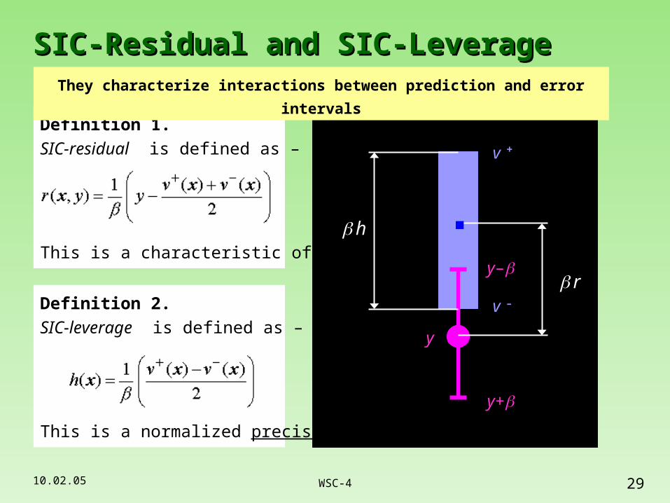
SIC-Residual and SIC-LeverageSIC-Residual and SIC-Leverage
Definition 1.
SIC-residual is defined as –
This is a characteristic of bias
Definition 2.
SIC-leverage is defined as –
This is a normalized precision
r
h
They characterize interactions between prediction and error intervals
10.02.05 30WSC-4
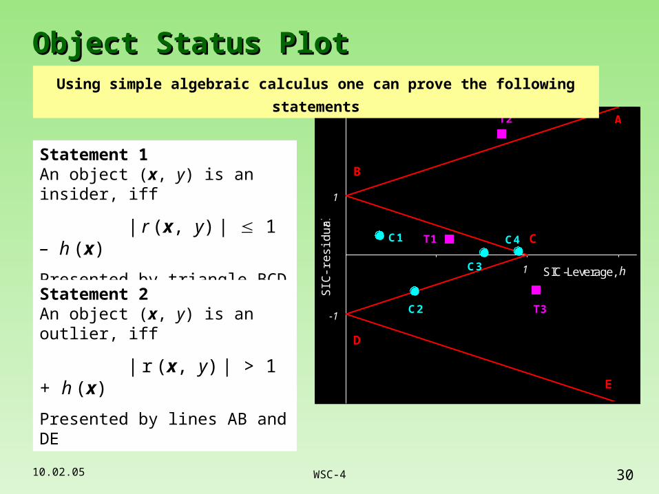
Object Status PlotObject Status Plot
1
-1
C1
C2
C3
C4
1
T1
T3
T2
SIC-Leverage, h
SIC
-res
idua
l, r
A
B
C
D
E
1
-1
C4
C3
C2
C1
1
T2
T3
T1
SIC-Leverage, h
SIC
-res
idua
l, r
A
B
C
D
E
1
-1
C4
C3
C2
C1
1
T2
T3
T1
SIC-Leverage, h
SIC
-res
idua
l, r
A
B
C
D
E
Statement 1 An object (x, y) is an insider, iff
| r (x, y) | 1 – h (x)
Presented by triangle BCD
Statement 2 An object (x, y) is an outlier, iff
| r (x, y) | > 1 + h (x)
Presented by lines AB and DE
Using simple algebraic calculus one can prove the following statements
10.02.05 31WSC-4
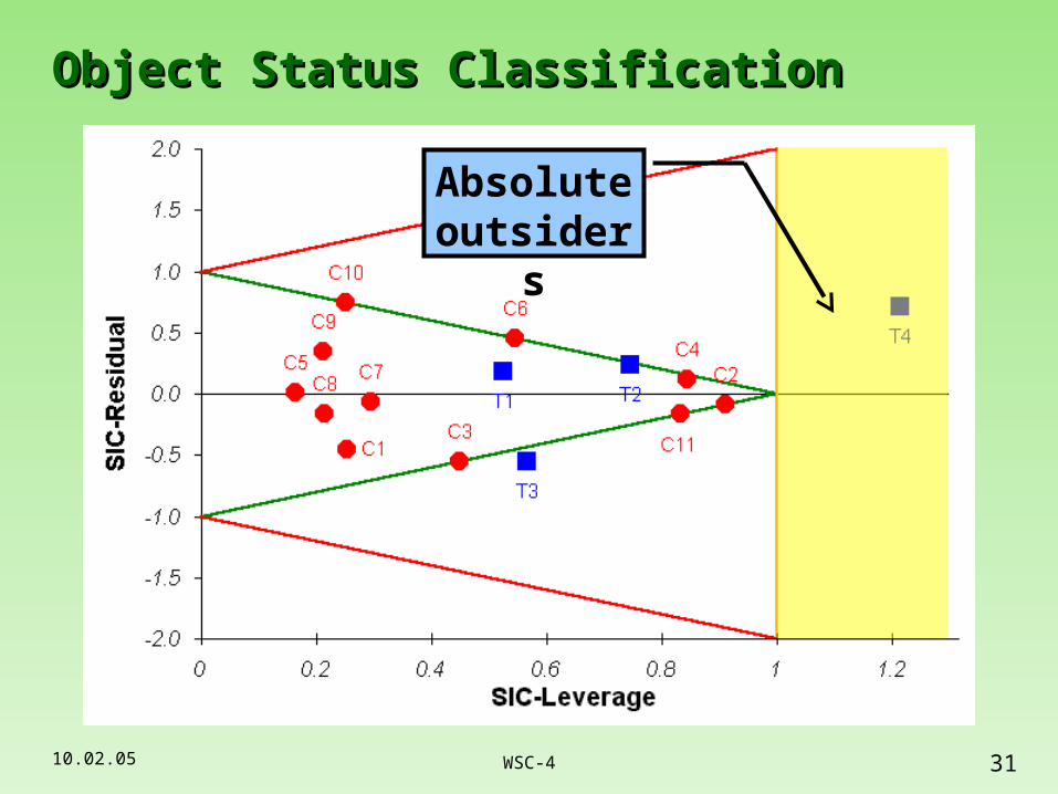
Insiders
Outsiders
OutliersAbsoluteoutsiders
Object Status ClassificationObject Status Classification
10.02.05 32WSC-4
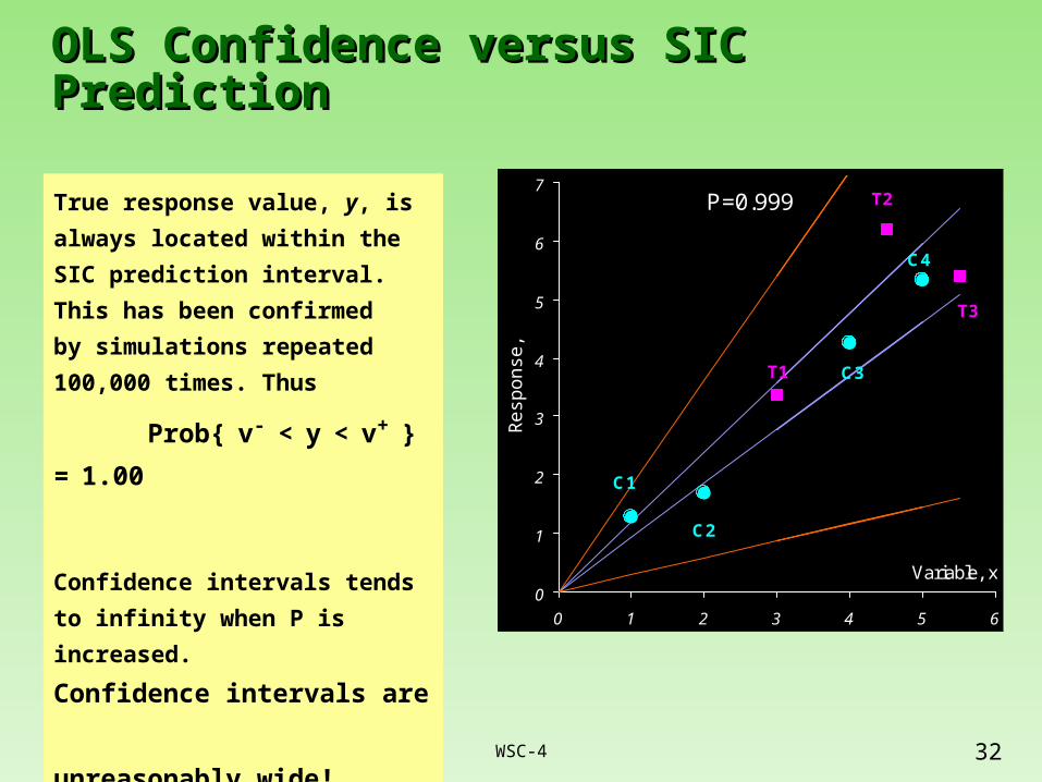
OLS Confidence versus SIC PredictionOLS Confidence versus SIC Prediction
P=0.95
C4
C3
C2
C1
T2
T3
T1
0
1
2
3
4
5
6
7
0 1 2 3 4 5 6
Variable, x
Res
pons
e, y
P=0.99
C1
C2
C3
C4
T1
T3
T2
0
1
2
3
4
5
6
7
0 1 2 3 4 5 6
Variable, x
Res
pons
e, y
P=0.999
C1
C2
C3
C4
T1
T3
T2
0
1
2
3
4
5
6
7
0 1 2 3 4 5 6
Variable, x
Res
pons
e, y
True response value, y, is always
located within the SIC prediction
interval. This has been confirmed
by simulations repeated 100,000
times. Thus
Prob{ v- < y < v+ } = 1.00
Confidence intervals tends to
infinity when P is increased.
Confidence intervals are
unreasonably wide!
10.02.05 33WSC-4
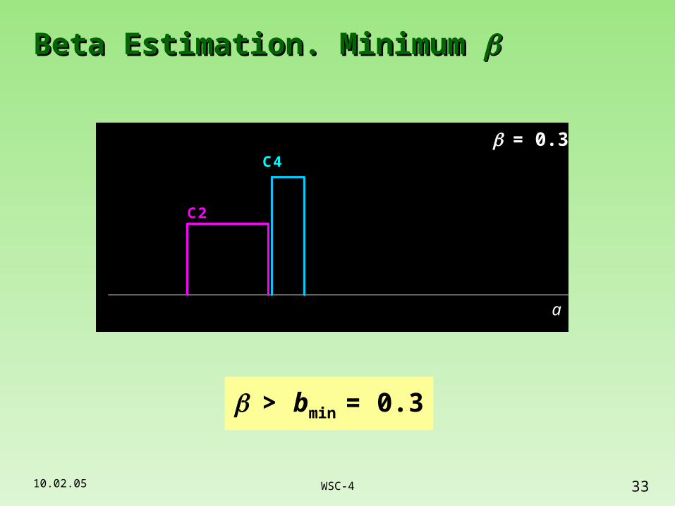
Beta Estimation. Minimum Beta Estimation. Minimum
C1
C2C3
C4
aRPV
= 0.7
C1
C2C3
C4
aRPV
= 0.6
C1
C2C3
C4
aRPV
= 0.5
C1
C2C3
C4
aRPV
= 0.4
C1
C2C3
C4
a
= 0.3
C2
C4
a
= 0.3
> bmin = 0.3
10.02.05 34WSC-4
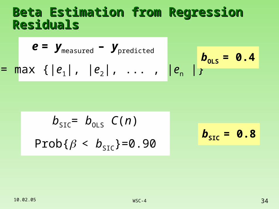
Beta Estimation from Regression ResidualsBeta Estimation from Regression Residuals
e = ymeasured – ypredicted
bOLS= max {|e1|, |e2|, ... , |en |}bOLS = 0.4
bSIC= bOLS C(n)
Prob{< bSIC}=0.90bSIC = 0.8
10.02.05 35WSC-4
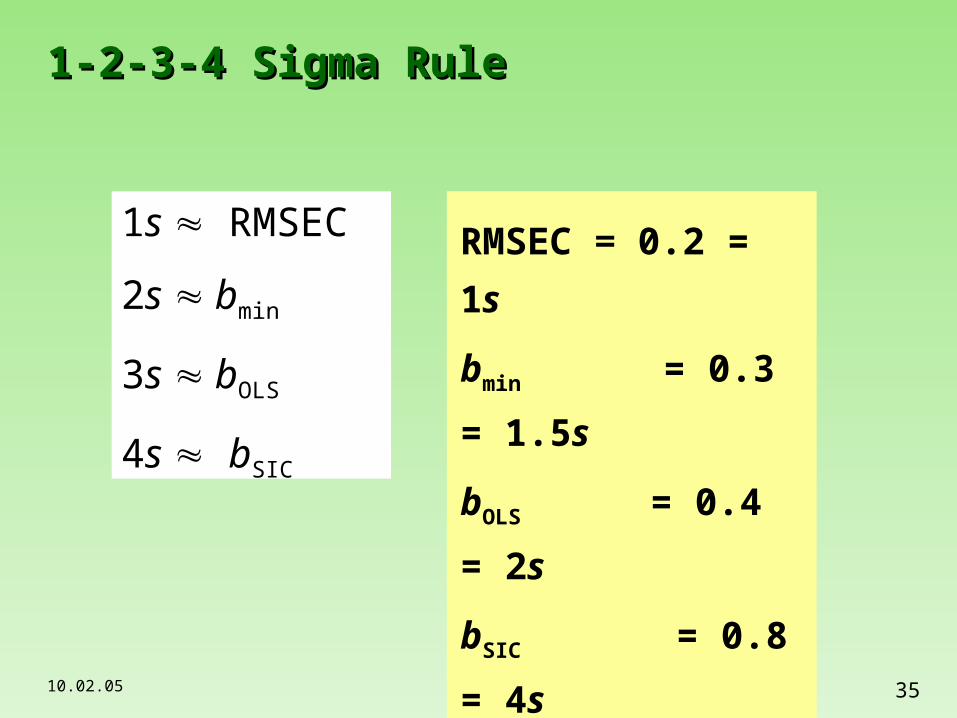
1-2-3-4 Sigma Rule1-2-3-4 Sigma Rule
1s RMSEC
2s bmin
3s bOLS
4s bSIC
RMSEC = 0.2 = 1s
bmin = 0.3 = 1.5s
bOLS = 0.4 = 2s
bSIC = 0.8 = 4s
10.02.05 36WSC-4
Part 3. Complicated SIC. Bivariate casePart 3. Complicated SIC. Bivariate case
10.02.05 37WSC-4
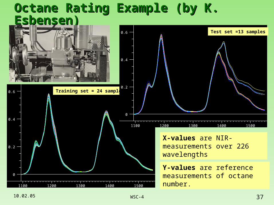
Octane Rating Example (by K. Esbensen)Octane Rating Example (by K. Esbensen)
X-values are NIR-measurements over 226 wavelengths
0
0.2
0.4
0.6
1100 1200 1300 1400 1500
Training set = 24 samples
0
0.2
0.4
0.6
1100 1200 1300 1400 1500
Test set =13 samples
Y-values are reference measurements of octane number.
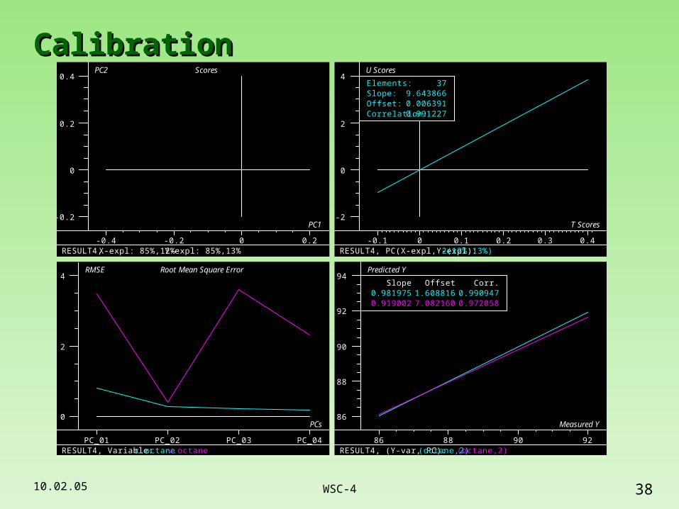
10.02.05 38WSC-4
CalibrationCalibration
-0.2
0
0.2
0.4
-0.4 -0.2 0 0.2
RESULT4, X-expl: 85%,12% Y-expl: 85%,13%
PC1
PC2 Scores
-2
0
2
4
-0.1 0 0.1 0.2 0.3 0.4
RESULT4, PC(X-expl,Y-expl): 2(12%,13%)
Elements:Slope:Offset:Correlation:
379.6438660.0063910.991227
T Scores
U Scores
0
2
4
PC_01 PC_02 PC_03 PC_04
RESULT4, Variable: c.octane v.octane
PCs
RMSE Root Mean Square Error
86
88
90
92
94
86 88 90 92
RESULT4, (Y-var, PC): (octane,2) (octane,2)
Slope Offset Corr.0.981975 1.608816 0.9909470.919002 7.082160 0.972058
Measured Y
Predicted Y
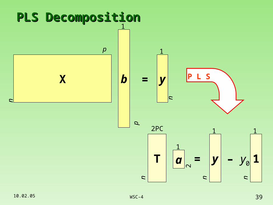
10.02.05 39WSC-4
PLS DecompositionPLS Decompositionn
X b y=
p
p
1
1
n
2PC
T a =
n
2
1
y
n
1
– y0 1
n
1
P L S
10.02.05 40WSC-4
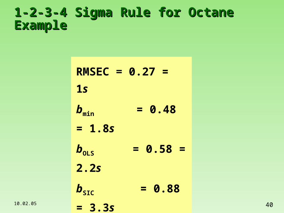
1-2-3-4 Sigma Rule for Octane Example1-2-3-4 Sigma Rule for Octane Example
RMSEC = 0.27 = 1s
bmin = 0.48 = 1.8s
bOLS = 0.58 = 2.2s
bSIC = 0.88 = 3.3s
= bSIC = 0.88
10.02.05 41WSC-4
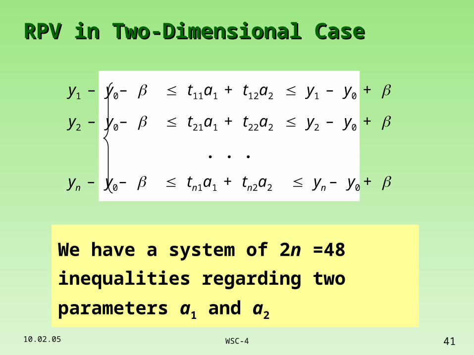
RPV in Two-Dimensional CaseRPV in Two-Dimensional Case
y1 – y0– t11a1 + t12a2 y1 – y0 +
y2 – y0– t21a1 + t22a2 y2 – y0 +
. . .
yn – y0– tn1a1 + tn2a2 yn – y0 +
We have a system of 2n =48 inequalities
regarding two parameters a1 and a2
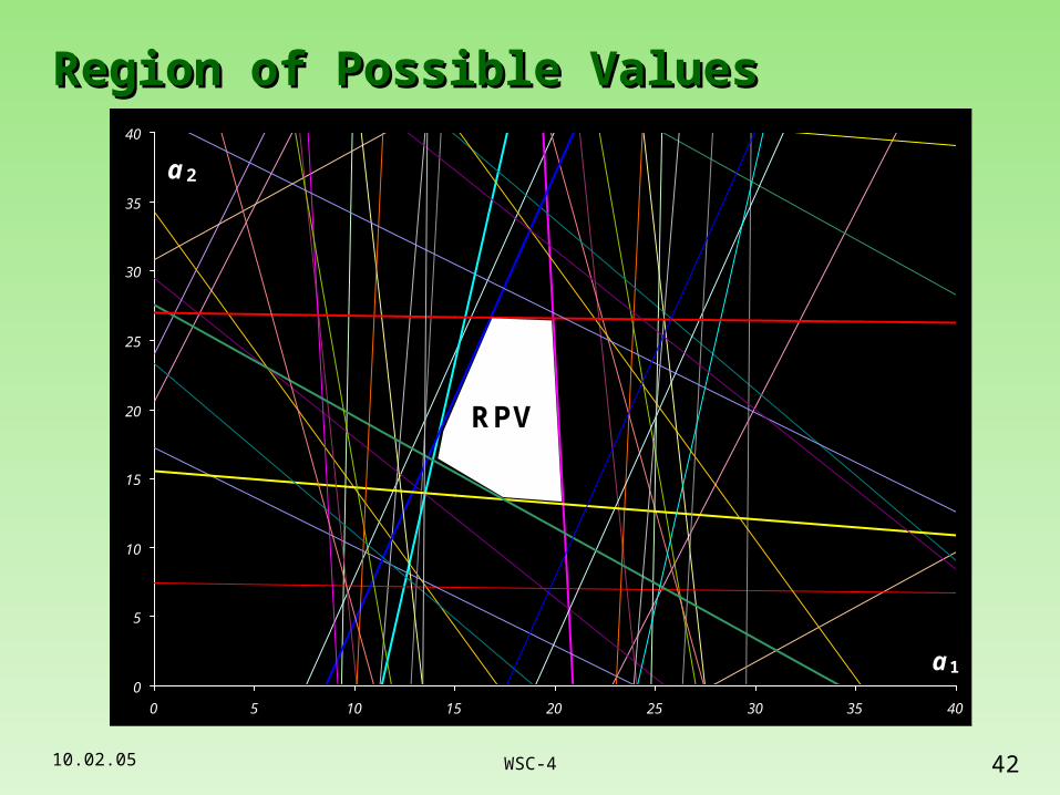
10.02.05 42WSC-4
0
5
10
15
20
25
30
35
40
0 5 10 15 20 25 30 35 40
a 1
a 2
Region of Possible ValuesRegion of Possible Values
0
5
10
15
20
25
30
35
40
0 5 10 15 20 25 30 35 40
a 1
a 2
0
5
10
15
20
25
30
35
40
0 5 10 15 20 25 30 35 40
a 1
a 2
0
5
10
15
20
25
30
35
40
0 5 10 15 20 25 30 35 40
a 1
a 2
0
5
10
15
20
25
30
35
40
0 5 10 15 20 25 30 35 40
a 1
a 2
0
5
10
15
20
25
30
35
40
0 5 10 15 20 25 30 35 40
a 1
a 2
0
5
10
15
20
25
30
35
40
0 5 10 15 20 25 30 35 40
a 1
a 2
RPV
10.02.05 43WSC-4
Close view on RPV. Calibration SetClose view on RPV. Calibration Set
24
232221
20
19
18
1716
15
14
13
12
11
10
9
8
7
6
5
4
3
2
1
-1
0
1
0 1
SIC-Leverage
SIC
-Re
sid
ua
l
Samples Boundary Samples
24C7 C9 C13 C14 C18 C23
—— —— —— —— —— ——
18+
9–
14–
13+
7+
23–
1
2
3
6 5
4
1
12
16
20
24
28
12 14 16 18 20 22
a 1
a 2
RPV
RPV in parameter space Object Status Plot
10.02.05 44WSC-4
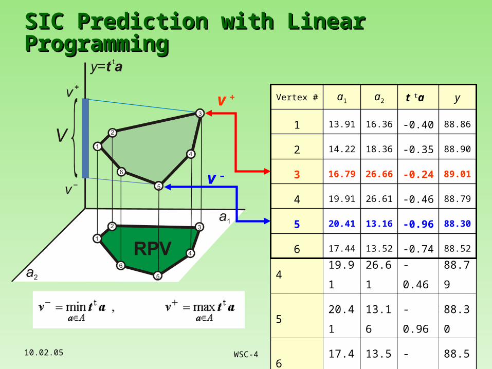
v –
SIC Prediction with Linear Programming SIC Prediction with Linear Programming
Linear Programming Problem
Vertex # a1 a2 t ta y
1 13.91 16.36 -0.40 88.86
2 14.22 18.36 -0.35 88.90
3 16.79 26.66 -0.24 89.01
4 19.91 26.61 -0.46 88.79
5 20.41 13.16 -0.96 88.30
6 17.44 13.52 -0.74 88.5288.52-0.7413.5217.446
88.30-0.9613.1620.415
88.79-0.4626.6119.914
89.01-0.2426.6616.793
88.90-0.3518.3614.222
88.86-0.4016.3613.911
yt ta a2a1Vertex #v +
10.02.05 45WSC-4
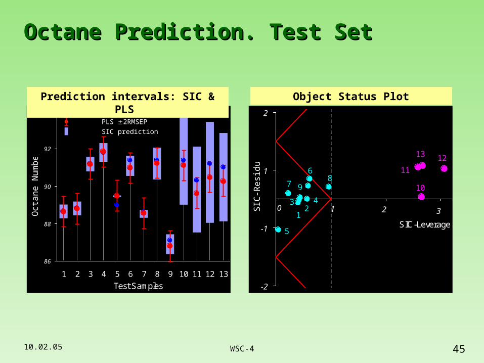
Octane Prediction. Test SetOctane Prediction. Test Set
86
88
90
92
94
1 2 3 4 5 6 7 8 9 10 11 12 13
Test Samples
Oct
ane
Num
ber
Reference values
PLS 2RMSEP
SIC prediction
5
86
9
2
7
43
1
11
13 12
10
3210
-2
-1
1
2
SIC-Leverage
SIC
-Res
idua
l
Prediction intervals: SIC & PLS Object Status Plot
10.02.05 46WSC-4
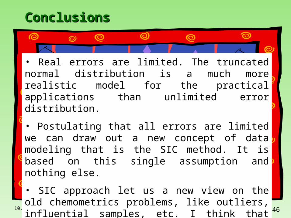
ConclusionsConclusions
• Real errors are limited. The truncated normal distribution is a much more realistic model for the practical applications than unlimited error distribution.
• Postulating that all errors are limited we can draw out a new concept of data modeling that is the SIC method. It is based on this single assumption and nothing else.
• SIC approach let us a new view on the old chemometrics problems, like outliers, influential samples, etc. I think that this is interesting and helpful view.
10.02.05 47WSC-4
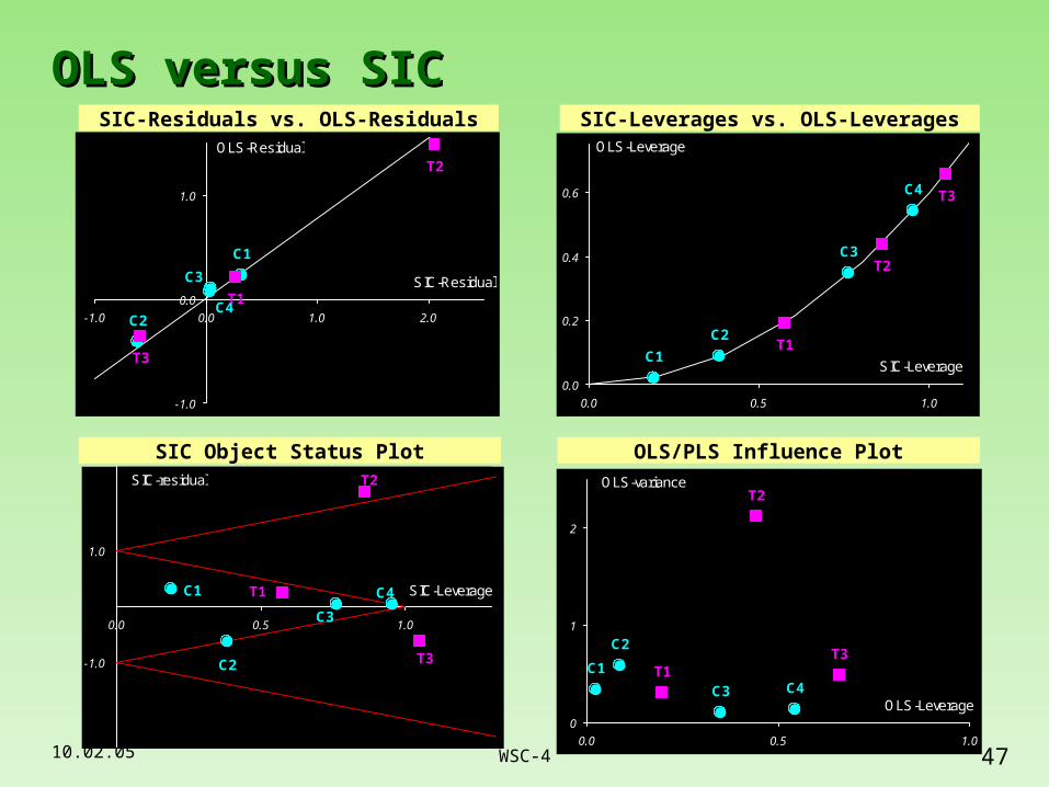
OLS versus SICOLS versus SIC
SIC-residual
C1
C2
C3
C4T1
T3
T2
-1.0
1.0
0.0 0.5 1.0
SIC-Leverage
OLS-variance
C4C3
C2
C1
T2
T3T1
0
1
2
0.0 0.5 1.0
OLS-Leverage
OLS-Leverage
C4
C3
C2
C1
T2
T3
T1
0.0
0.2
0.4
0.6
0.0 0.5 1.0
SIC-Leverage
OLS-Residual
C1
C2
C3
C4T1
T3
T2
-1.0
0.0
1.0
-1.0 0.0 1.0 2.0
SIC-Residual
SIC-Residuals vs. OLS-Residuals SIC-Leverages vs. OLS-Leverages
SIC Object Status Plot OLS/PLS Influence Plot
10.02.05 48WSC-4
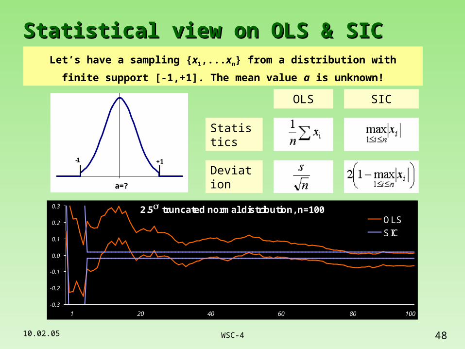
Statistical view on OLS & SIC Statistical view on OLS & SIC
OLS SIC
Statistics
Deviation
Let’s have a sampling {x1,...xn} from a distribution with finite support [-1,+1].
The mean value a is unknown!
+1-1
a=?
2.5 truncated normal distribution, n=100
1 20 40 60 80 100
-0.3
-0.2
-0.1
0.0
0.1
0.2
0.3
OLS
SIC