Embed Size (px)
Citation preview
Geomorphology 10. Portage County Glacial Landforms
K.A. Lemke – UWSP 65
10. PORTAGE COUNTY GLACIAL LANDFORMS
80 Points (30 Trip; 50 Questions)
The objective of this lab exercise is to explore the glacial landforms in Portage County via a field trip where we can see these landforms firsthand, and through examination and analysis of information on topographic and geologic maps.
YOU SHOULD BE ABLE TO:
• Identify the glacial landforms found in Portage County, WI in the field and on topographic maps, including end moraines, outwash plains, ice-walled lake deposits, tunnel channels, and outwash fans;
• Describe the characteristics of these glacial landforms using information from topographic maps and field observations; • Compare and contrast the characteristics and formation processes of these landforms; • Explain where we would expect to find these landforms in relation to one another and how the relative geographic
position of landforms may be indicative of their age; and • Describe specific differences and similarities between the end moraines of the last glacial advance (Hancock and
Almond Phases) and the end moraines of the much earlier Arnott Phase in Portage County.
INTRODUCTION
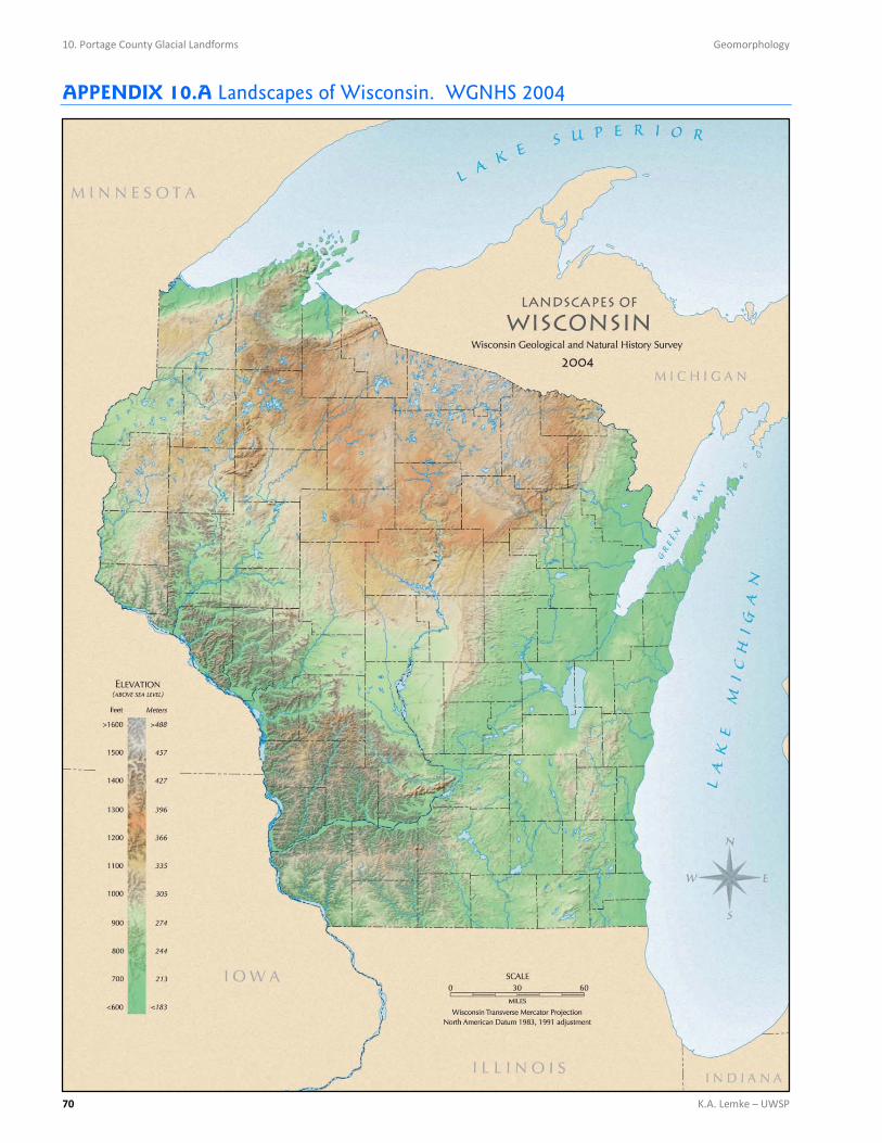
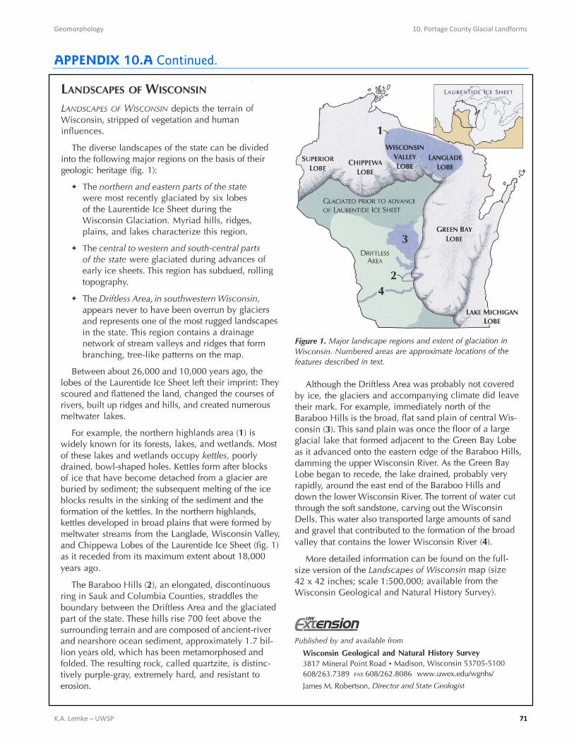
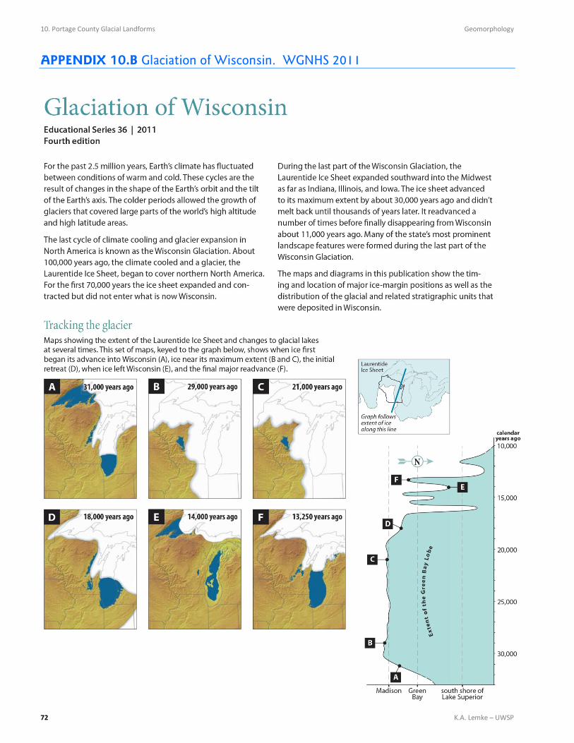
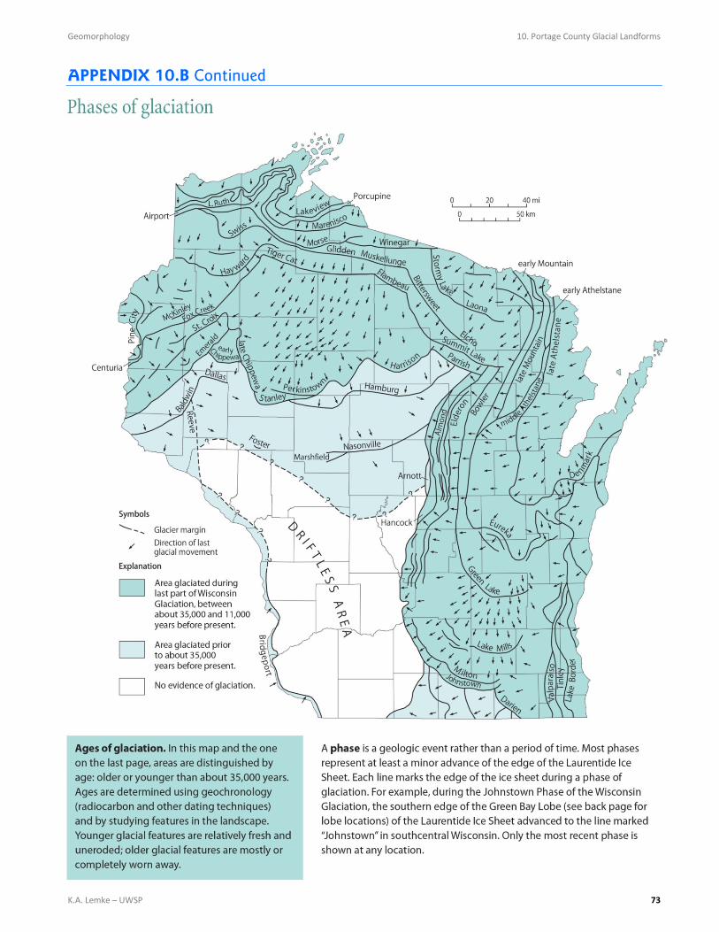
The last, large scale advance of glaciers during the Wisconsin Glaciation, called the late Wisconsin, began approximately 25,000 YBP (Years Before Present). During the late Wisconsin, the Green Bay Lobe (see Appendix 10.A for a map of glacial lobes in Wisconsin) advanced into Portage County and created a variety of landforms as the terminus of the glacier advanced or retreated, remained stationary or stagnated. The topography of central Wisconsin clearly reflects its glacial heritage. The terminal moraine from the last glacial advance, as well as a portion of a terminal moraine from an earlier advance are clearly visible on the landscape (see Appendix 10.A. Landscapes of Wisconsin). Phases refer to geologic events not to a particular time period (WGNHS 2011). A number of phases (events) occurred while the ice was in Portage County. In the field we will view landforms associated with the Arnott, Hancock, and Almond Phases (see Appendix 10.B Phases of Glaciation). In stratigraphy, a formation refers to a stratigraphic unit that covers a large spatial area, that has similar lithology, texture, color, and other physical characteristics throughout the entire extent of the unit, and that occupies a specific stratigraphic position (NACSN 2005). The glacial deposits in Portage County from the Green Bay Lobe are part of the Holy Hill Formation (Figure 10.1). The Holy Hill Formation includes the Horicon Member, the Keene Member, and undifferentiated sand
FIGURE 10.1 Stratigraphic Units of Portage County (Clayton 1986, p. 2, Figure 2)
Horicon Member
Keene Member
Hillslope Sediment
Cambrian & Precambrian
Rock
Undifferentiated Sediment
HOLY HILL FORMATION
10. Portage County Glacial Landforms Geomorphology
66 K.A. Lemke – UWSP
and gravel. The very southwestern portion of Portage County contains deposits of the Big Flats Formation, deposits primarily associated with Glacial Lake Wisconsin (not marked on Figure 10.1; WGNHS 2011). See Appendix 10.B for a map and chart of the glacial formations (lithostratigraphic units) in Wisconsin. The northwestern corner of Portage County contains hillslope deposits (Figure 10.1). These are primarily mass movement deposits derived from materials formed as local rock weathered in place (Clayton 1986). Although parts of northwestern Portage County may have been glaciated at some time in the distant past, there is little evidence of this glaciation remaining within Portage County today.
THE HOLY HILL FORMATION
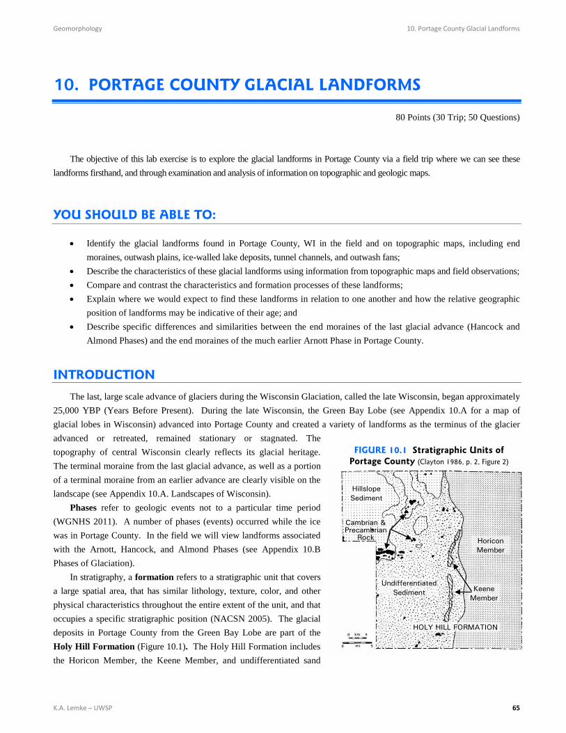
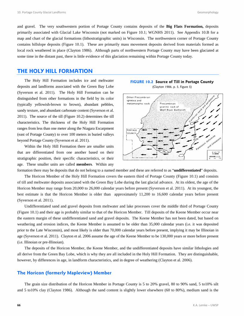
The Holy Hill Formation includes ice and meltwater deposits and landforms associated with the Green Bay Lobe (Syverson et al. 2011). The Holy Hill Formation can be distinguished from other formations in the field by its color (typically yellowish-brown to brown), abundant pebbles, sandy texture, and abundant carbonate content (Syverson et al. 2011). The source of the till (Figure 10.2) determines the till characteristics. The thickness of the Holy Hill Formation ranges from less than one meter along the Niagara Escarpment (east of Portage County) to over 100 meters in buried valleys beyond Portage County (Syverson et al. 2011). Within the Holy Hill Formation there are smaller units that are differentiated from one another based on their stratigraphic position, their specific characteristics, or their age. These smaller units are called members. Within any formation there may be deposits that do not belong to a named member and these are referred to as “undifferentiated” deposits. The Horicon Member of the Holy Hill Formation covers the eastern third of Portage County (Figure 10.1) and consists of till and meltwater deposits associated with the Green Bay Lobe during the last glacial advance. At its oldest, the age of the Horicon Member may range from 20,000 to 26,000 calendar years before present (Syverson et al. 2011). At its youngest, the best estimate is that the Horicon Member is older than approximately 11,200 to 16,600 calendar years before present (Syverson et al. 2011). Undifferentiated sand and gravel deposits from meltwater and lake processes cover the middle third of Portage County (Figure 10.1) and their age is probably similar to that of the Horicon Member. Till deposits of the Keene Member occur near the eastern margin of these undifferentiated sand and gravel deposits. The Keene Member has not been dated, but based on weathering and erosion indices, the Keene Member is assumed to be older than 35,000 calendar years (i.e. it was deposited prior to the Late Wisconsin), and most likely is older than 70,000 calendar years before present, implying it may be Illinoian in age (Syverson et al. 2011). Clayton et al. 2006 assume the age of the Keene Member to be 130,000 years or more before present (i.e. Illinoian or pre-Illinoian). The deposits of the Horicon Member, the Keene Member, and the undifferentiated deposits have similar lithologies and all derive from the Green Bay Lobe, which is why they are all included in the Holy Hill Formation. They are distinguishable, however, by differences in age, in landform characteristics, and in degree of weathering (Clayton et al. 2006).
The Horicon (formerly Mapleview) Member
The grain size distribution of the Horicon Member in Portage County is 5 to 20% gravel, 80 to 90% sand, 5 to10% silt and 5 to10% clay (Clayton 1986). Although the sand content is slightly lower elsewhere (60 to 80%), medium sand is the
FIGURE 10.2 Source of Till in Portage County (Clayton 1986, p. 5, Figure 5)
Geomorphology 10. Portage County Glacial Landforms
K.A. Lemke – UWSP 67
dominant grain size (Clayton 1986, Syverson et al.2011). The Horicon Member is brown and unstratified (Syverson et al. 2011). In Portage County, pink granitic rock derived from the Wolf River Batholith (Figure 10.2) is a major component of the coarser clasts and some surface boulders attain sizes up to two meters in diameter (Clayton 1986). Carbonate material (dolomite) occurs primarily in the sand and gravel fractions of the till (Clayton 1986). On average, carbonates have been leached to a depth of 2 m (Clayton 1986). The Kewaunee Formation overlies the Horicon Member in the Green Bay area (see Appendix 10.2 map of Pleistocene lithostratigraphic units). These two units are distinguishable by the much redder color and finer texture of the Kewaunee Formation (Syverson et al. 2011). The Horicon Member is distinguishable from the Keene Member based on differences in texture, degree of weathering, appearance, and stratigraphic position (Syverson et al. 2011). The Horicon Member presumably overlies the Keene Member in eastern Portage County (Syverson et al. 2011). Key end moraines of the Horicon Member include the Hancock Moraine, a relatively continuous terminal moraine formed during the Hancock Phase (about 16,500 YBP), and the Almond Moraine, a relatively continuous recessional moraine formed during the Almond Phase (about 15, 750 YBP) (Clayton et al. 2006). There are other smaller and less continuous recessional moraines that formed during the Elderon Phase (about 15, 000 YBP) (Clayton et al. 2006). The average width of the Hancock moraine is one kilometer and the height varies from 6 to 21 meters. The average width of the Almond moraine is 0.5 kilometers and the height varies from 5 to 18 meters (Clayton 1986). Both of these moraines can be traced (see Appendix 10.A) almost continuously to the north into Langlade County and to the south where they correlate to the Johnstown and Milton moraines in Dane County (Clayton 1986). The thickness of the till in both end moraines is unknown but is sufficiently thick to mask underlying, preexisting landforms; it is most likely as thick as the moraines are high (Clayton 1986). Ground moraine occurs sporadically behind theses end moraines. This till is thinner than the till of the end moraines and does not mask the preexisting underlying topography (Clayton 1986). In places, the till has been eroded away or covered by meltwater sediment. The ground moraine till may be difficult to distinguish from meltwater sediment because of the high sand content of both types of deposits (Clayton 1986).
The Keene Member
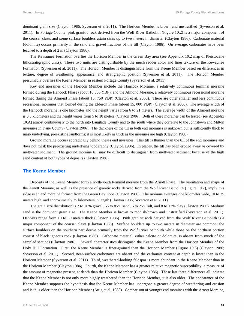
Deposits of the Keene Member form a north-south terminal moraine from the Arnott Phase. The orientation and shape of the Arnott Moraine, as well as the presence of granitic rocks derived from the Wolf River Batholith (Figure 10.2), imply this ridge is an end moraine formed from the Green Bay Lobe (Clayton 1986). The moraine averages one kilometer wide, 10 to 25 meters high, and approximately 25 kilometers in length (Clayton 1986; Syverson et al. 2011). The grain size distribution is 2 to 20% gravel, 65 to 85% sand, 5 to 25% silt, and 8 to 17% clay (Clayton 1986). Medium sand is the dominant grain size. The Keene Member is brown to reddish-brown and unstratified (Syverson et al. 2011). Deposits range from 10 to 30 meters thick (Clayton 1986). Pink granitic rock derived from the Wolf River Batholith is a major component of the coarser clasts (Clayton 1986). Surface boulders up to two meters in diameter are common; the surface boulders on the southern part derive primarily from the Wolf River batholith while those on the northern portion consist of black igneous rock (Clayton 1986). Carbonate material, either calcite or dolomite, is absent from much of the sampled sections (Clayton 1986). Several characteristics distinguish the Keene Member from the Horicon Member of the Holy Hill Formation. First, the Keene Member is finer-grained than the Horicon Member (Figure 10.3) (Clayton 1986; Syverson et al. 2011). Second, near-surface carbonates are absent and the carbonate content at depth is lower than in the Horicon Member (Syverson et al. 2011). Third, weathered-looking feldspar is more abundant in the Keene Member than in the Horicon Member (Clayton 1986). Fourth, the Keene Member has a greater relative magnetic susceptibility, a measure of the amount of magnetite present, at depth than the Horicon Member (Clayton 1986). These last three differences all indicate that the Keene Member is not only more highly weathered than the Horicon Member, it is also older. The appearance of the Keene Member supports the hypothesis that the Keene Member has undergone a greater degree of weathering and erosion and is thus older than the Horicon Member (Attig et al. 1988). Comparison of younger end moraines with the Arnott Moraine,
10. Portage County Glacial Landforms Geomorphology
68 K.A. Lemke – UWSP
either on topographic maps or in the field, reveals the Arnott Moraine has a much smoother surface; no hummocks or undrained depressions exist on the Arnott Moraine while both of these features occur abundantly on the younger moraines. This implies more erosion has occurred on the Arnott Moraine, smoothing its surface (Clayton 1986), which in turn implies a longer degree of exposure to the elements and thus an older age.
Undifferentiated Sediment
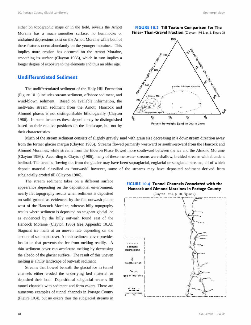
The undifferentiated sediment of the Holy Hill Formation (Figure 10.1) includes stream sediment, offshore sediment, and wind-blown sediment. Based on available information, the meltwater stream sediment from the Arnott, Hancock and Almond phases is not distinguishable lithologically (Clayton 1986). In some instances these deposits may be distinguished based on their relative positions on the landscape, but not by their characteristics. Much of the stream sediment consists of slightly gravely sand with grain size decreasing in a downstream direction away from the former glacier margin (Clayton 1986). Streams flowed primarily westward or southwestward from the Hancock and Almond Moraines, while streams from the Elderon Phase flowed more southward between the ice and the Almond Moraine (Clayton 1986). According to Clayton (1986), many of these meltwater streams were shallow, braided streams with abundant bedload. The streams flowing out from the glacier may have been supraglacial, englacial or subglacial streams, all of which deposit material classified as “outwash” however, some of the streams may have deposited sediment derived from subglacially eroded till (Clayton 1986). The stream sediment takes on a different surface appearance depending on the depositional environment: nearly flat topography results when sediment is deposited on solid ground as evidenced by the flat outwash plains west of the Hancock Moraine, whereas hilly topography results where sediment is deposited on stagnant glacial ice as evidenced by the hilly outwash found east of the Hancock Moraine (Clayton 1986) (see Appendix 10.A). Stagnant ice melts at an uneven rate depending on the amount of sediment cover. A thick sediment cover provides insulation that prevents the ice from melting readily. A thin sediment cover can accelerate melting by decreasing the albedo of the glacier surface. The result of this uneven melting is a hilly landscape of outwash sediment. Streams that flowed beneath the glacial ice in tunnel channels either eroded the underlying bed material or deposited their load. Depositional subglacial streams fill tunnel channels with sediment and form eskers. There are numerous examples of tunnel channels in Portage County (Figure 10.4), but no eskers thus the subglacial streams in
FIGURE 10.3 Till Texture Comparison For The Finer- Than-Gravel Fraction (Clayton 1986, p. 3, Figure 3)
FIGURE 10.4 Tunnel Channels Associated with the Hancock and Almond Moraines in Portage County
(Clayton 1986, p. 10, Figure 9)
Geomorphology 10. Portage County Glacial Landforms
K.A. Lemke – UWSP 69
Portage County eroded underlying bed material (Clayton 1986). Tunnel channels formed at the ice margin during the Hancock and Almond phases. Rows of collapse depressions, breaks through the end moraines, and large outwash fans beyond the moraine indicate the location of tunnel channels (Clayton 1986). Clayton et al. (1985) suggest that a 10 km wide swath along the glacier margin was frozen to its bed, and behind the frozen bed zone a narrow thawed bed zone existed. Sudden discharge of accumulated meltwater from the thawed bed zone through the frozen bed zone may have been responsible for the formation of the tunnel channels (Clayton 1986). Offshore sediment, or sediment deposited in lakes, comprise the remainder of the undifferentiated fluvial sediment. The primary grain size transported by the glacial ice was sand, and thus the offshore sediment is primarily sand; silt and clay are not common (Clayton 1986). Lakes occurred along the margin of the glacier as the ice dammed water flow, but some also occurred as ice-walled lakes. These ice-walled lakes formed flat-topped mounds known as ice walled lake plains.
THE BIG FLATS FORMATION
The Big Flats Formation (see Appendix 10.B map of lithostratigraphic units) is composed of stream sediment and sediment associated with Glacial Lake Wisconsin (Syverson et al. 2011). Since this formation consists of old lake bed sediment, the topography is quite flat (see Appendix 10.A). as the sediment is an ancient lake bed. The deposit is composed almost entirely of medium and fine sand that is well-sorted and stratified with a dark grayish-brown to dark yellowish-brown color (Syverson et al. 2011). Sand in the Big Flats Formation can be distinguished from sand in the Holy Hill Formation by its color, the fact that it is more well-sorted, and the lack of coarse sand and gravel (Syverson et al. 2011). Variations in grain size distribution within the Big Flats Formation is a function of the depositional environment – stream, beach, nearshore and offshore. The offshore deposits include layers of silt and clay (Syverson et al. 2011). The thickness ranges from one to over forty meters (Syverson et al. 2011). The surface layers to the formation were deposited between 16,000 to 24,000 calendar years before present (Syverson et al. 2011). Wind-blown sand was deposited on top of the Big Flats Formation during the Holocene and a widespread paleosol separates the fluvial sand from the overlying aeolian sand (Syverson et al. 2011).
REFERENCES
Attig, J.W., L. Clayton, and D.M. Mickelson, eds. 1988. Pleistocene Stratigraphic Units of Wisconsin 1984-1987. Wisconsin Geological and Natural History Survey Information Circular 62. Madison: WGNHS.
Clayton, L. 1986. Pleistocene Geology of Portage County, Wisconsin. Wisconsin Geological and Natural History Survey Information Circular 56. Madison: WGNHS.
Clayton, L., J.W. Attig, D.M. Mickelson, M.D. Johnson, and K.M. Syverson. 2006. Glaciation of Wisconsin, 3rd ed. Wisconsin Geological and Natural History Survey Educational Series 36. Madison: WGNHS.
NACSN (North American Commission on Stratigraphic Nomenclature). 2005. North American stratigraphic code. American Association of Petroleum Geologists (AAPG) Bulletin 89(11):1547-1591, doi:10.1306/07050504129.
Syverson, K.M., L. Clayton, J.W. Attig, and D.M. Mickelson (eds). 2011. Lexicon of Pleistocene Stratigraphic Units of Wisconsin. Wisconsin Geological and Natural History Survey Technical Report 1. Madison: WGNHS.
WGNHS (Wisconsin Geological and Natural History Survey). 1983. Thickness of Unconsolidated Material in Wisconsin. Madison: WGNHS.
WGNHS (Wisconsin Geological and Natural History Survey). 2004. Landscapes of Wisconsin. Madison: WGNHS. WGNHS (Wisconsin Geological and Natural History Survey). 2011. Glaciation of Wisconsin (4th ed). Wisconsin Geological
and Natural History Survey Educational Series 36. Madison: WGNHS.
10. Portage County Glacial Landforms Geomorphology
70 K.A. Lemke – UWSP
APPENDIX 10.A Landscapes of Wisconsin. WGNHS 2004
Geomorphology 10. Portage County Glacial Landforms
K.A. Lemke – UWSP 71
APPENDIX 10.A Continued.
10. Portage County Glacial Landforms Geomorphology
72 K.A. Lemke – UWSP
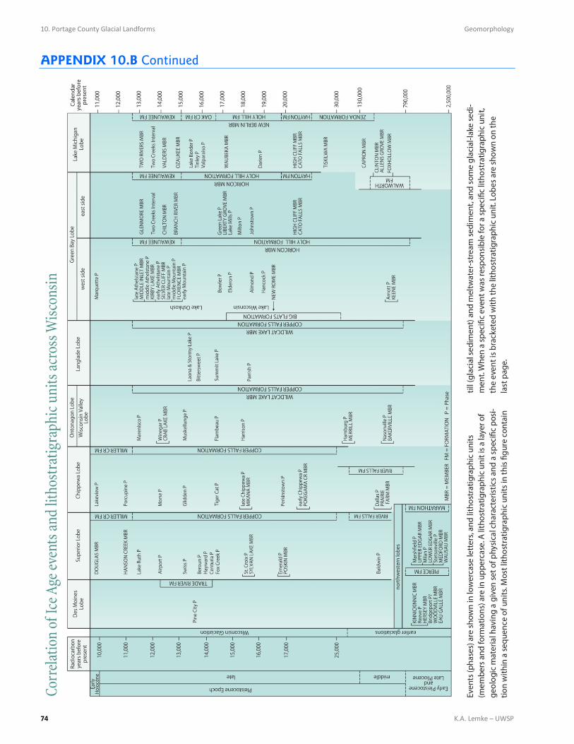
APPENDIX 10.B Glaciation of Wisconsin. WGNHS 2011
Geomorphology 10. Portage County Glacial Landforms
K.A. Lemke – UWSP 73
APPENDIX 10.B Continued
10. Portage County Glacial Landforms Geomorphology
74 K.A. Lemke – UWSP
APPENDIX 10.B Continued
Geomorphology 10. Portage County Glacial Landforms
K.A. Lemke – UWSP 75
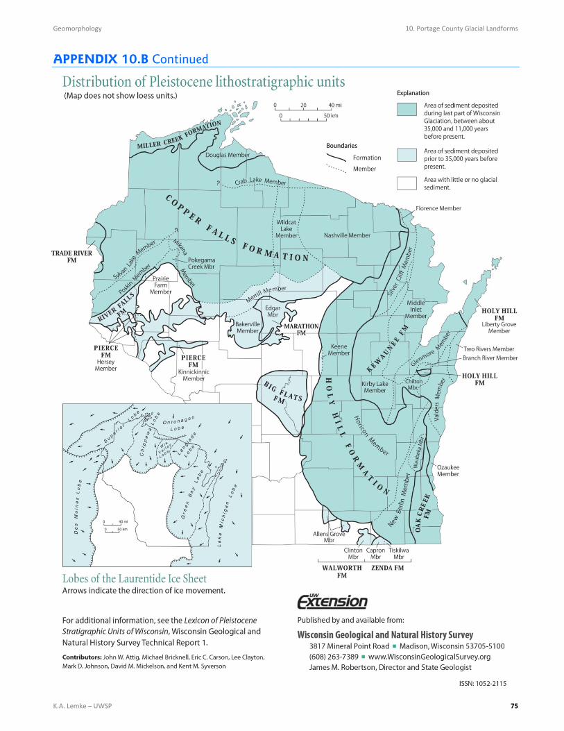
APPENDIX 10.B Continued
10. Portage County Glacial Landforms Geomorphology
76 K.A. Lemke – UWSP
PROCEDURE
This exercise has two parts, the first part is the actual field trip and the second part involves working with topographic and geologic maps of the areas we visit on the field trip. Part 1: We will take 2 hours to visit five or six stops that will allow us to see three end moraines, the Hancock and Almond from the last glacial advance, and the Arnott from an earlier advance. We will also get a view of hilly till, an outwash fan, and the outwash plain east of Stevens Point. You are expected to take notes during the field trip and mark the location of our stops on the topographic maps associated with this lab exercise. Making notes on your topographic maps in the field will make the second part of the exercise easier. Failure to attend the field trip will result in zero points; there will be no make-up field trip. Part 2: This part involves answering the questions associated with this exercise. You will need to hand in your answers to those questions as well as your topographic maps.
Geomorphology 10. Portage County Glacial Landforms
K.A. Lemke – UWSP 77
10. PORTAGE COUNTY GLACIAL LANDFORMS
Dimensions of the Hancock Moraine
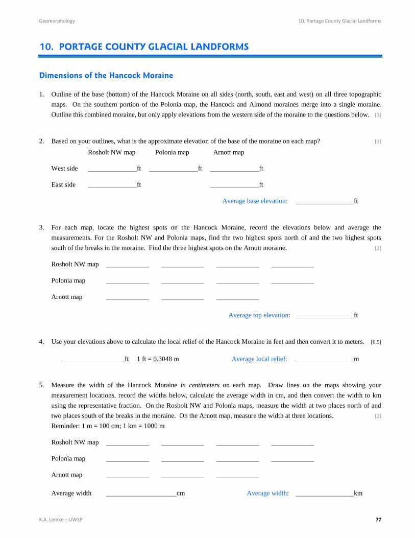
1. Outline of the base (bottom) of the Hancock Moraine on all sides (north, south, east and west) on all three topographic maps. On the southern portion of the Polonia map, the Hancock and Almond moraines merge into a single moraine. Outline this combined moraine, but only apply elevations from the western side of the moraine to the questions below. [3]
2. Based on your outlines, what is the approximate elevation of the base of the moraine on each map? [1]
Rosholt NW map Polonia map Arnott map
West side ft ft ft
East side ft ft
Average base elevation: ft
3. For each map, locate the highest spots on the Hancock Moraine, record the elevations below and average the measurements. For the Rosholt NW and Polonia maps, find the two highest spots north of and the two highest spots south of the breaks in the moraine. Find the three highest spots on the Arnott moraine. [2]
Rosholt NW map
Polonia map
Arnott map
Average top elevation: ft
4. Use your elevations above to calculate the local relief of the Hancock Moraine in feet and then convert it to meters. [0.5]
ft 1 ft = 0.3048 m Average local relief: m
5. Measure the width of the Hancock Moraine in centimeters on each map. Draw lines on the maps showing your measurement locations, record the widths below, calculate the average width in cm, and then convert the width to km using the representative fraction. On the Rosholt NW and Polonia maps, measure the width at two places north of and two places south of the breaks in the moraine. On the Arnott map, measure the width at three locations. [2]
Reminder: 1 m = 100 cm; 1 km = 1000 m
Rosholt NW map
Polonia map
Arnott map
Average width cm Average width: km
10. Portage County Glacial Landforms Geomorphology
78 K.A. Lemke – UWSP
6. Compare your height (local relief) and width measurements to the averages of Clayton, 1986 (refer to Introduction)? [0.5]
Moraine height (m): yours: Clayton’s
Moraine width (km) yours: Clayton’s
If your measurements are not in the range of Clayton’s, list some reasons why this might be the case.
Dimensions of the Almond Moraine
7. The Almond Moraine appears as a distinct moraine on the Rosholt NW map only. Outline the base (bottom) of the Almond Moraine on all sides on the topographic map. The northern-most portions of the moraine are difficult to define, particularly on the eastern side. Draw unclear boundaries as dashed lines. [1]
8. Based on your outlines, what is the approximate elevation of the base of the moraine on the: [0.5]
west side? ft east side? ft Average base elevation: ft
9. Locate the four highest spots on the southern portion of the Almond Moraine where the moraine is clearly defined. Locate two other high spots from the northern, less-well defined portions of the Almond moraine. Record these six elevations below. [1]
Average top elevation: ft
10. Use your elevations above to calculate the local relief of the Almond Moraine in feet and then convert it to meters. [0.5]
ft 1 ft = 0.3048 m Average local relief: m
11. On the Rosholt NW map, measure the width in centimeters of the Almond Moraine at four locations on the southern portion of the Almond Moraine where the moraine is clearly defined) and at two locations from the northern, less-well defined portions of the moraine. Draw lines on the maps showing your measurement locations, record the widths below, calculate the average width in cm, and then convert the width to km using the representative fraction. [1.5]
Average width cm Average width: km
Geomorphology 10. Portage County Glacial Landforms
K.A. Lemke – UWSP 79
12. Compare your height and width measurements to the averages of Clayton, 1986 (refer to Introduction)? [0.5]
Moraine height (m): yours: Clayton’s
Moraine width (km) yours: Clayton’s
If your measurements are not in the range of Clayton’s, list some reasons why this might be the case.
Dimensions of the Arnott Moraine
13. On the Arnott topographic map draw the outline of the base (bottom) of the Arnott Moraine on all sides. [1]
14. Based on your outlines, what is the approximate: [0.5]
West side base elevation? ft East side base elevation? ft
15. Locate the four highest spots on the top of the Arnott Moraine and record these elevations below. [1]
Elevations (ft):
Average top elevation: ft
16. Use your elevations above to calculate the local relief of the Arnott Moraine in feet and then convert it to meters. [1]
West side local relief: ft West side local relief m
East side local relief: ft East side local relief m
17. Measure the width in centimeters of the Arnott Moraine in four places. One measurement should be at the widest part of the moraine and one should be the narrowest part of the moraine. The other two are at your discretion. Draw lines on the maps showing your measurement locations, record the widths below, calculate the average width in cm, and then convert the width to km using the representative fraction. [1]
Widths (cm):
Average width cm Average width: km
10. Portage County Glacial Landforms Geomorphology
80 K.A. Lemke – UWSP
18. Compare your height and width measurements to the averages of Clayton, 1986 (refer to Introduction)? [0.5]
Moraine height (m): yours: Clayton’s
Moraine width (km) yours: Clayton’s
If your measurements are not in the range of Clayton’s, list some reasons why this might be the case.
Comparison of the End Moraines
19. Summarize your moraine measurements below. Base elevation (ft) Top Local West Side East Side Elevation (ft) Relief (m) Width (km)
Arnott
Hancock
Almond
Compare and contrast the elevations, local relief, and widths of the three moraines by identifying similarities and differences. Then identify trends in the measurements from west to east. [4]

Geomorphology 10. Portage County Glacial Landforms
K.A. Lemke – UWSP 81
20. a. Highlight (or color) any depressions (closed contour lines with hatch marks) located on the Hancock, Almond, and Arnott moraines on all three topographic maps. [1]
b. Compare and contrast the frequency of depressions on these three moraines. [2]
21. Examine the shape of the contour lines (i.e. squiggles, irregularities, places where lines double back, the ease of following a specific line) within each of your moraine outlines. Compare and contrast the shape (squigglyness) of the contour lines on the three moraines. [2]
22. Examine the spacing of the contour lines (i.e. the horizontal distance separating neighboring contour lines) on all three moraines. Compare and contrast the amount of space separating neighboring contour lines and the consistency of the spacing between neighboring contour lines on the three moraines. [2]
23. Because the base elevation on the west side of the Arnott Moraine is lower than on the east side, the local relief of the Arnott Moraine is larger on the west side than on the east side. What might have caused the higher base elevation, and thus the lower local relief, on the east side of this moraine? [2]
10. Portage County Glacial Landforms Geomorphology
82 K.A. Lemke – UWSP
24. Based on the information in the introduction, on the topographic maps, and from our field trip, list other similarities and differences between the Hancock, Almond and Arnott moraines. [4]
25. If you had no information on the age of the Arnott, Hancock and Almond moraines, how could you determine their relative ages based solely on their geographic position on the landscape? [1]
26. If you had no information on the age of these three moraines, and you didn’t know their geographic position on the landscape, what other information collected in this exercise could you use to determine their relative ages? [1]
Tunnel Channels
Tunnel channels form where meltwater from the thawed-bed zone of the glacier erodes a tunnel through the frozen-bed zone of the glacier and then flows out onto the outwash plain fronting the glacier. The tunnel may be carved out of the underlying sediment or the ice itself. According to Clayton (1986) three features signifying the location of a tunnel channel: (1) rows of collapse depressions, (2) breaks in end moraines, and (3) proglacial fans.
27. On the Polonia map there is a break between the northern and southern portion of the Hancock and Almond moraines and your outlines from questions 1 and 7 should show this break. There are a series of depressions (closed contour lines with hatch marks) in the break and to the east of the break. Mark these depressions on the map to help show the location of the tunnel channel that drained through this break in the moraine. [1]
Geomorphology 10. Portage County Glacial Landforms
K.A. Lemke – UWSP 83
28. In addition to depressions, the location of this tunnel channel is also signified by a trough (valley) and the contour lines help define this trough to the east of the break in the moraine. Examine the contour lines to the east of the break and mark the approximate edges of the valley that defines the old tunnel channel. Draw an arrow along the bottom of this old channel, through the depression contours and out through the break in the moraine showing the direction of water flow when the glacier was present. [1.5]
29. Highlight several of the contour lines defining the proglacial fan that formed at the end of the tunnel channel where meltwater flowed out onto the outwash plain. [1]
30. Examine the elevation of the contour lines on the outwash fan, at the break in the moraine, and through the trough (valley) behind the moraine.
a. Today, the highest elevation along this old tunnel channel marks a drainage divide. Where is the highest elevation today, in front of the moraine on the outwash fan, at the break in the moraine, or behind the moraine where the ice was? [0.25]
b. Given your answer, in what direction(s) will water drain off the landscape today? [0.25]
c. Is the direction of drainage today the same as the direction of drainage when the glacier was here? If the direction of flow today is different than when the ice was present, explain how this could be the case. [1.5]
31. How do we know that the tunnel channels are younger than the moraines they cut through? [1]
Topography and Geology
32. On the Rosholt NW and Polonia topographic maps highlight two or three examples of each of the following features. Use topography in conjunction with the glacial deposits map of Portage County to help identify these features. Create a key here. [2]
a. ground moraine c. hilly outwash (outwash deposited on stagnant ice)
b. flat outwash d. ice-walled lakes
The other major type of glacial landform in this area is end moraines, but these were all marked on the maps for earlier questions, so they don’t need to be marked again.
10. Portage County Glacial Landforms Geomorphology
84 K.A. Lemke – UWSP
33. How does the pattern (i.e. shape, spacing, number) of the contour lines differ between these five different types of landforms? In other words, if you didn’t have the geologic map to help you identify these landforms, what would you look for with regards to the pattern of the contour lines to determine their location? [4]