10 Algebraic Algorithms for Linear Matroid Parity Problemshoyeeche/papers/parity.pdf · 10 Algebraic Algorithms for Linear Matroid Parity Problems HO YEE CHEUNG, LAP CHI LAU, and

10

Algebraic Algorithms for Linear Matroid Parity Problems

HO YEE CHEUNG, LAP CHI LAU, and KAI MAN LEUNG, The Chinese University of Hong Kong

We present fast and simple algebraic algorithms for the linear matroid parity problem and its applications.For the linear matroid parity problem, we obtain a simple randomized algorithm with running time O(mrω−1),where mand r are the number of columns and the number of rows, respectively, and ω ≈ 2.3727 is the matrixmultiplication exponent. This improves the O(mrω)-time algorithm by Gabow and Stallmann and matchesthe running time of the algebraic algorithm for linear matroid intersection, answering a question of Harvey.We also present a very simple alternative algorithm with running time O(mr2), which does not need fastmatrix multiplication.

We further improve the algebraic algorithms for some specific graph problems of interest. For the Mader’sdisjoint S-path problem, we present an O(nω)-time randomized algorithm where n is the number of vertices.This improves the running time of the existing results considerably and matches the running time of thealgebraic algorithms for graph matching. For the graphic matroid parity problem, we give an O(n4)-timerandomized algorithm where n is the number of vertices, and an O(n3)-time randomized algorithm for aspecial case useful in designing approximation algorithms. These algorithms are optimal in terms of n asthe input size could be �(n4) and �(n3), respectively.

The techniques are based on the algebraic algorithmic framework developed by Mucha and Sankowski,Harvey, and Sankowski. While linear matroid parity and Mader’s disjoint S-path are challenging gener-alizations for the design of combinatorial algorithms, our results show that both the algebraic algorithmsfor linear matroid intersection and graph matching can be extended nicely to more general settings. Allalgorithms are still faster than the existing algorithms even if fast matrix multiplication is not used. Theseprovide simple algorithms that can be easily implemented in practice.

Categories and Subject Descriptors: F.2.2 [Analysis of Algorithms and Problem Complexity]: Non-numerical Algorithms and Problems; G.2.1 [Discrete Mathematics]: Combinatorics—Combinatorialalgorithms; G.2.2 [Discrete Mathematics]: Graph Theory—Graph algorithms

General Terms: Algorithms, Theory

Additional Key Words and Phrases: Matroid parity

ACM Reference Format:Ho Yee Cheung, Lap Chi Lau, and Kai Man Leung. 2014. Algebraic algorithms for linear matroid parityproblems. ACM Trans. Algor. 10, 3, Article 10 (April 2014), 26 pages.DOI: http://dx.doi.org/10.1145/2601066

A preliminary version of the article appeared in Proceedings of the 22nd ACM-SIAM Symposium on DiscreteAlgorithms (SODA), 2011.This research is supported by RGC grant 412907 and GRF grant 413609 from the Research Grant Councilof Hong Kong.Authors’ addresses: H. Y. Cheung, Computer Science Department, University of Southern California, 941Bloom Walk, Los Angeles, CA 90089-0781, United States; email: [email protected]; L. C. Lau,Department of Computer Science and Engineering, The Chinese University of Hong Kong, Shatin, HongKong; email: [email protected]; K. M. Leung, Department of Computer Science and Engineering, TheChinese University of Hong Kong, Shatin, Hong Kong; email: [email protected] to make digital or hard copies of part or all of this work for personal or classroom use is grantedwithout fee provided that copies are not made or distributed for profit or commercial advantage and thatcopies show this notice on the first page or initial screen of a display along with the full citation. Copyrights forcomponents of this work owned by others than ACM must be honored. Abstracting with credit is permitted.To copy otherwise, to republish, to post on servers, to redistribute to lists, or to use any component of thiswork in other works requires prior specific permission and/or a fee. Permissions may be requested fromPublications Dept., ACM, Inc., 2 Penn Plaza, Suite 701, New York, NY 10121-0701 USA, fax +1 (212)869-0481, or [email protected]© 2014 ACM 1549-6325/2014/04-ART10 $15.00

DOI: http://dx.doi.org/10.1145/2601066

ACM Transactions on Algorithms, Vol. 10, No. 3, Article 10, Publication date: April 2014.

http://dx.doi.org/10.1145/2601066

http://dx.doi.org/10.1145/2601066

10:2 H. Y. Cheung et al.

1. INTRODUCTION

The graph matching problem and the matroid intersection problem are two fundamen-tal polynomial-time-solvable problems in combinatorial optimization. Several effortshave been made to obtain an elegant common generalization of these two problems,for example, the matroid parity problem by Lawler [1976] (equivalent to the matchoidproblem by Edmonds [Jenkyns 1974] and the matroid matching problem by Lovasz[1980]), the optimal path-matching problem by Cunningham and Geelen [1997], andthe membership problem for jump system by Bouchet and Cunningham [1995, 1997].

So far the matroid parity problem is the most-studied and the most fruitful prob-lem among these generalizations. Although it is shown to be intractable in the oraclemodel [Jensen and Korte 1982] and is NP hard for matroids with compact representa-tions [Lovasz 1980], Lovasz [1980] proved an exact min-max formula and obtained apolynomial time algorithm for the linear matroid parity problem.

This provides a polynomial-time-solvable common generalization of the graph match-ing problem and the linear matroid intersection problem.1 Moreover, the linear matroidparity problem has many applications of its own in various areas, including the pathpacking problem [Mader 1978; Schrijver 2003] in combinatorial optimization, the min-imum pinning set problem [Lovasz 1980; Jordan 2010] in combinatorial rigidity, themaximum genus imbedding problem [Furst et al. 1988] in topological graph theory,the graphic matroid parity problem [Lovasz 1980; Gabow and Stallmann 1985] usedin approximating minimum Steiner tree [Promel and Steger 1997; Berman et al. 2006]and approximating maximum planar subgraph [Calinescu et al. 1998], and the uniquesolution problem [Lovasz and Plummer 1986] in electric circuit.

Given its generality and applicability, it is thus of interest to obtain fast algorithmsfor the linear matroid parity problem. In this article, we will present faster and sim-pler algorithms for the linear matroid parity problem and also improved algorithmsfor specific graph problems of interest. The algorithms are based on the algebraicalgorithmic framework developed by Mucha and Sankowski [2004], Harvey [2009,2007], and Sankowski [2006].

1.1. Problem Formulation and Previous Work

The linear matroid parity problem can be formulated as follows without using termi-nology from matroid theory:2 Given an r×2mmatrix where the columns are partitionedinto m pairs, find a maximum cardinality collection of pairs so that the union of thecolumns of these pairs is linearly independent. For instance, to formulate the graphmatching problem as a linear matroid parity problem, we construct an n × 2m ma-trix where the rows are indexed by the vertices and the pairs are indexed by theedges, where an edge i j is represented by two columns where one column has a 1 inthe ith entry and 0 otherwise and the other column has a 1 in the jth entry and 0otherwise.

There are several deterministic combinatorial algorithms for the linear matroid par-ity problem. The first polynomial time algorithm is obtained by Lovasz with a runningtime of O(m17), which can be implemented to run in O(m10) time [Lovasz 1980; Lovaszand Plummer 1986]. The fastest known algorithm is an augmenting path algorithmobtained by Gabow and Stallmann [1986] with running time O(mrω) [Schrijver 2003],where ω ≈ 2.3727 is the exponent on the running time of the fastest known matrixmultiplication algorithm [Stothers 2010; Vassilevska Williams 2 012]. Orlin and Vande

1This only holds when both matroids are representable over the same field, but it covers most of theapplications of the matroid intersection problem; see Section 4 of Harvey [2009] for more discussions.2It is not necessary to formulate the general matroid parity problem for this article, but the formulation andsome background of matroid theory will be provided in Section 3.


Algebraic Algorithms for Linear Matroid Parity Problems 10:3

Vate [1990] presented an algorithm with running time O(mrω+1) [Schrijver 2003] byreducing it to a sequence of matroid intersection problems. Recently, Orlin [2008] pre-sented a simpler algorithm with running time O(mr3). While these algorithms are alldeterministic and reveal substantial structural insights into the problem, even the sim-plest algorithm by Orlin is quite complex and probably too difficult to be implementedin practice.

On the other hand, Lovasz [1979] proposed an algebraic approach to the linear ma-troid parity problem. First, he constructed an appropriate matrix with indeterminates(variables) where the matrix is of full rank if and only if there are r/2 linearly indepen-dent pairs (see Section 4.1). Then he showed that determining whether the matrix isof full rank can be done efficiently with high probability, by substituting the variableswith independent random values from a large enough field, and then computing thedeterminant of the resulting matrix [Lovasz 1979]. This approach can be easily modi-fied to determine the optimal value of the linear matroid parity problem in one matrixmultiplication time, and one can also construct a solution in m matrix multiplicationstime. Note that this already gives a randomized O(mrω)-time algorithm for the linearmatroid parity problem, and this algebraic approach also leads to an efficient parallelalgorithm for the linear matroid parity problem [Narayanan et al. 1994].

In a recent line of research, an elegant algorithmic framework has been developedfor this algebraic approach. Mucha and Sankowski [2004] showed how to use Gaussianeliminations to construct a maximum matching in one matrix multiplication time,leading to an O(nω)-time algorithm for the graph matching problem where n is thenumber of vertices. Harvey [2009] used a divide-and-conquer method to obtain analgebraic algorithm for the linear matroid intersection problem with running timeO(mrω−1), where m is the number of columns, and a simple O(nω)-time algorithmfor the graph matching problem. Furthermore, Sankowski [2006] and Harvey [2007]extended the algebraic approach to obtain faster pseudo-polynomial algorithms for theweighted bipartite matching problem and the weighted linear matroid intersectionproblem.

Besides matching and linear matroid intersection, other special cases of the linearmatroid parity problem have also been studied. One special case of interest is thegraphic matroid parity problem [Gabow and Stallmann 1985; Gabow and Xu 1989;Szigeti 1998, 2003], which has applications in designing approximation algorithms[Calinescu et al. 1998; Promel and Steger 1997; Berman et al. 2006]. For this prob-lem, the fastest known algorithm is by Gabow and Stallmann [1985], which runs inO(mn lg6 n) time. Another special problem of considerable interest is the Mader’s S-pathpacking problem [Mader 1978; Lovasz 1980; Sebo and Szego 2004; Chudnovsky et al.2008; Pap 2007a, 2007b, 2008; Babenko 2010] which is a generalization of the graphmatching problem and the s-t vertex disjoint path problem. Lovasz [1980] showed thatthis problem can be reduced to the linear matroid parity problem. Chudnovsky et al.[2008] obtained an O(n6)-time direct combinatorial algorithm for the problem, and Pap[2007b, 2008] obtained a simpler direct combinatorial algorithm for the problem andalso for the more general capacitated setting.

1.2. Our Results

We obtain fast and simple algebraic algorithms for the linear matroid parity problemand also for some specific graph problems of interest. All algorithms are best possiblein the sense that either they match the running time in well-known special cases orthey are optimal in terms of some parameters.

1.2.1. Linear Matroid Parity. There are two algebraic formulations for the linear matroidparity problem; one is a “compact” formulation (Theorem 4.1) by Lovasz [1979] and the



other is a “sparse” formulation (Theorem 4.2) by Geelen and Iwata [2005]. Using thecompact formulation and the Sherman-Morrison-Woodbury formula, we present a verysimple algorithm for the linear matroid parity problem.

THEOREM 1.1. There is an O(mr2)-time randomized algorithm for the linear matroidparity problem.

One feature of this algorithm is that it does not use fast matrix multiplication andis very easy to be implemented in practice. Note that it is already faster than theGabow-Stallmann O(mrω) time algorithm, and actually if fast matrix multiplication isnot used, then the best- known algorithms run in O(mr3) time [Gabow and Stallmann1986; Orlin 2008]. Using the divide-and-conquer method of Harvey [2009] on the sparseformulation and fast matrix multiplications, we can improve the running time furtherto match the running time of the linear matroid intersection problem, answering aquestion of Harvey [2009].

THEOREM 1.2. There is an O(mrω−1)-time randomized algorithm for the linear matroidparity problem.

We present a faster pseudo-polynomial randomized algorithm for the weighted ma-troid parity problem, which has time complexity O(Wmrω). This also implies a fasterrandomized FPTAS for the weighted linear matroid parity problem using standardscaling technique [Promel and Steger 1997].

1.2.2. Graph Algorithms. For graph problems that can be reduced to the linear matroidparity problem, we show that the additional structure can be exploited in the compactformulation to obtain faster algorithms than those that follow from Theorem 1.2. Weillustrate this with some well-known problems.

Mader’s Disjoint S-Path. In this problem, we are given an undirected graph G =(V, E) and S is a collection of disjoint subsets of V , and the goal is to find a maxi-mum collection of vertex disjoint S-paths, where an S-path is a path that connectstwo different sets in S and has no internal vertex in S. This problem generalizes thegraph matching problem and the vertex disjoint s-t path problem, and is of consid-erable interest [Mader 1978; Lovasz 1980; Sebo and Szego 2004; Chudnovsky et al.2008; Pap 2007a, 2007b, 2008; Babenko 2010]. Obtaining a direct combinatorial algo-rithm is quite nontrivial [Chudnovsky et al. 2008; Pap 2008]. The best-known runningtime is still the O(mnω)-time bound implied by the Gabow-Stallmann algorithm, wherem is the number of edges and n is the number of vertices. The algorithm in Theorem 1.2implies an O(mnω−1)-time algorithm. By using the compact formulation, we furtherimprove the running time to match the algebraic algorithms for the graph match-ing problem. The algorithm would be quite simple if fast matrix multiplication is notused, and its running time would be O(n3), which is still faster than the existingalgorithms.

THEOREM 1.3. There is an O(nω)-time randomized algorithm for the Mader’s S-pathproblem.

Graphic Matroid Parity. In this problem, we are given an undirected graph andsome edge pairs, and the problem is to find a maximum collection of edge pairs suchthat the union of these edges forms a forest. One special case of interest [Lovasz andPlummer 1986; Szigeti 1998] is when each pair has a common vertex (i.e., {i j, ik} forsome vertex i). This has applications in approximating minimum Steiner tree [Promel



and Steger 1997; Berman et al. 2006] and approximating maximum planar subgraph[Calinescu et al. 1998]. In the general problem, the input could have up to �(n4) edgepairs where n is the number of vertices, and in the special problem, the number of edgepairs could be �(n3). The following algorithms achieve optimal running time in termsof n for both problems.

THEOREM 1.4. There is an O(n4)-time randomized algorithm for the graphic matroidparity problem, and an O(n3)-time randomized algorithm when each edge pair has acommon vertex.

The fastest algorithm on graphic matroid parity is obtained by Gabow and Stallmann[1985] with running time O(mn lg6 n), where m is the number of edge pairs, and so ouralgorithm is faster if there are �(n3) edge pairs in the general problem and if thereare �(n2) edge pairs in the special problem. We remark that the same statement holdseven if we use a cubic algorithm for matrix multiplication, and the resulting algorithmis much simpler than that of Gabow and Stallmann.

Colorful Spanning Tree. In this problem, we are given an undirected multigraphG = (V, E), where each edge has one color, and the objective is to determine whetherthere is a spanning tree in which every edge has a distinct color. This is a generalizationof the arborescence problem and the connected detachment problem [Nash-Williams1985; Schrijver 2003] and is a special case of the linear matroid intersection problem.Note that the input graph could have �(n3) edges, where n is the number of vertices,since each pair of vertices could have �(n) edges in between, each of which has a distinctcolor. So the following algorithm has optimal running time in terms of n.

THEOREM 1.5. There is an O(n3)-time randomized algorithm for the colorful spanningtree problem.

1.3. Techniques

Our results show that both the algebraic algorithms for graph matching and linearmatroid intersection can be generalized to linear matroid parity. The O(mrω−1)-timealgorithm for linear matroid parity is a straightforward generalization of Harvey’slinear matroid intersection algorithm, and the algorithm for weighted linear matroidparity follows from the techniques used by Sankowski [2006]. The main new techni-cal contribution is the use of the compact formulation to design new algebraic algo-rithms. For graph problems, the basic observation is that the column vectors have atmost a constant number of nonzeros, and this allows us to extend Harvey’s matchingalgorithm and small area update formula to obtain faster algorithms using the com-pact formulation. The O(nω) algorithm for the S-path problem is based on a goodmatrix formulation of the problem, while the O(n3) algorithms for graphic matroidparity and colorful spanning tree are based on different recursions used in thedivide-and-conquer method. We remark that this approach on the compact formu-lation implies some new results for linear matroid intersection problems as well,for example, colorful spanning tree, graphic matroid intersection, and simple O(mr2)algorithm.

While linear matroid parity and Mader’s disjoint S-path are challenging generaliza-tions for the design of combinatorial algorithms, our results show that the algebraicalgorithmic framework can be adapted nicely to give faster and simpler algorithmsin more general settings. Our algorithms are still faster than the existing algorithmseven if fast matrix multiplications are not used, and these simpler algorithms could beimplemented easily in practice using MATLAB (see, e.g., Harvey [2008]).



2. ALGEBRAIC PRELIMINARIES

Notations: Given a matrix M, the submatrix containing rows S and columns T isdenoted by MS,T . A submatrix containing all rows (or columns) is denoted by M∗,T (orMS,∗), and an entry of M is denoted by Mi, j . Let �ei be a column vector with a 1 in theith position and 0 otherwise. When a set of integers S is partitioned into k subsets,the set S is partitioned into k equal-size subsets S1, S2, . . . Sk. In addition, S1 containsthe smallest |S|/k elements of S, S2 contains the next |S|/k smallest elements of S,and Sk contains the largest |S|/k elements of S.

Algebraic algorithms: Given two n × n matrices with entries in a field F ofsize poly(n), the matrix multiplication operation requires O(nω) time [Stothers 2010;Vassilevska Williams 2012], where ω < 2.3727. For an n×n matrix, it is known that theoperations of computing the determinant, computing the rank, computing the inverse,and computing a maximum rank submatrix can all be done in the same time boundas one matrix multiplication [Bunch and Hopcroft 1974; Harvey 2008]. We assume thenumber of pairs m and the number of rows r in the linear matroid parity problem willbe powers of two. This assumption can be easily satisfied by adding redundant pairsand rows.

Matrix of indeterminates: Let F be a field, and let F(x1, . . . , xm) be the field ofrational function over F with indeterminates {x1, x2, . . . , xm}. A matrix with entriesin F(x1, . . . , xm) is called a matrix of indeterminates. A matrix M of indeterminatesis nonsingular if and only if its determinant is not the zero function. To check if ann × n matrix M with indeterminates is nonsingular, one can substitute each xi witha random value in Fq and call the resulting matrix M′. Throughout this article, eachentry of M is a linear polynomial in x1, . . . , xm. Thus, by the Schwartz-Zippel Lemma, ifM is nonsingular, then det(M′) is zero with probability at most n/q. Hence, by settingq = nc for a large constant c, this gives a randomized algorithm with running timeO(nω) to test if M is nonsingular with high probability.

Skew-symmetric matrix: A matrix M is called skew symmetric if Mi, j = −Mj,i forall i, j. For any nonsingular skew-symmetric matrix M, it is known that its inverse isalso skew symmetric [Murota 2009].

Small rank update formula: Suppose we have a matrix M and its inverse M−1. Ifwe perform a small rank update on M, the following formula [Woodbury 1950] showshow to update M−1 efficiently.

LEMMA 2.1 (SHERMAN-MORRISON-WOODBURY). Let M be an n × n matrix, U be an n × kmatrix, and V be an n × k matrix. Suppose that M is nonsingular. Then

(1) M + U V T is nonsingular if and only if I + V T M−1U is nonsingular.(2) If M + U V T is nonsingular, then (M + U V T )−1 = M−1 − M−1U (I + V T

M−1U )−1V T M−1.

Small area update formula: Suppose we have a matrix M and its inverse M−1. Ifwe update MS,S for small |S|, then Harvey [2009] showed that the Sherman-Morrison-Woodbury formula can be used to compute the values in M−1

T ,T quickly for small|T |.

LEMMA 2.2 (HARVEY). Let M be a nonsingular matrix and let N = M−1. Let M be amatrix that is identical to M except MS,S �= MS,S and let � = M − M.

(1) M is nonsingular if and only if det(I + �S,S NS,S) �= 0.(2) If M is nonsingular, then M−1 = N − N∗,S(I + �S,S NS,S)−1�S,S NS,∗.(3) Restricting M−1 to a subset T , we have M−1

T ,T = NT ,T − NT ,S(I +�S,S NS,S)−1�S,S NS,T , and this can be computed in O(|T |ω) time for |T | ≥ |S|.



3. MATROID PRELIMINARIES

A matroid is a pair M = (V, I) of a finite set V and a set I of subsets of V so that thefollowing axioms are satisfied:

(1) ∅ ∈ I,(2) I ⊆ J ∈ I ⇒ I ∈ I, and(3) I, J ∈ I, |I| < |J| ⇒ ∃v ∈ J \ I such that I ∪ {v} ∈ I.

We call V the ground set and I ∈ I an independent set. So I is the family of independentsets. Bases B of M are independent sets with maximum size. By the aforementioneaxioms, all bases have the same size. For any U ⊆ V , the rank of U , denoted by rM(U ),is defined as

rM(U ) = max{|I||I ⊆ U, I ∈ I}.3.1. Examples

Linear Matroid. Let Z be a matrix over a field F and V be the set of the column vectorsof Z. The linear independence among the vectors of Z defines a matroid M on ground setV . A set I ⊆ V is independent in M if and only if the column vectors indexed by I arelinearly independent. The rank function r of M is simply defined as rM(I) = rank(Z∗,I).A matroid that can be obtained in this way is linearly representable over F.

Partition Matroid. Let {V1, . . . , Vk} be a partition of ground set V , that is,⋃k

i=1 Vi = Vand Vi ∩ Vj = ∅ for i �= j. Then the family of the independent sets I on the ground setV is given by

I = {I ⊆ V : |I ∩ Vi| ≤ 1 ∀i ∈ {1, . . . , k}}.M = (V, I) is called the partition matroid. Partition matroids are linearly repre-sentable. This can be done by representing each element v ∈ Vi as a vector �ei.

Graphic Matroid. Let G = (V, E) be a graph with vertex set V and edge set E. Agraphic matroid has ground set E. A set I ⊆ E is independent if and only if I containsno cycles in G. The matroid is linearly representable by representing each edge (u, v) ∈ Eto a column vector �eu − �ev in the linear matroid.

3.2. Constructions

The restriction of a matroid M to U ⊆ V , denoted as M|U , is a matroid with groundset U so that I ⊆ U is independent in M|U if and only if I is independent in M. Thisis the same as saying M|U is obtained by deleting the elements V \ U in M. The rankfunction rM|U of M|U is simply rM|U (I) = rM(I) for I ⊆ U .

The contraction of a matroid M by U ⊆ V , denoted by M/U , is a matroid on groundset V \ U so that I ⊆ V \ U is independent if and only if I ∪ B is independent in M fora base B of M|U . The rank function rM/U of M/U is given by

rM/U (I) = rM(I ∪ U ) − rM(U ), I ⊆ V \ U.

For any matrix Z and its corresponding linear matroid M, the matrix for M/{i} canbe obtained by Gaussian eliminations on Z as follows. First, using row operation andscaling, we can transform the column indexed by i to a unit vector �ek. Then the matrixobtained by removing the ith column and kth row from M is the required matrix. Itcan be seen that I ∪ {i} is independent in M if and only if I is independent in M/{i}.3.3. Matroid Parity

Given a matroid M = (V, I) whose elements are given in pairs where each elementis contained in exactly one pair, the matroid parity problem is to find a maximum



cardinality collection of pairs, so that union of these pairs is an independent set ofM. The general matroid parity problem is intractable in the oracle model [Jensen andKorte 1982] and is NP hard on matroids with compact representations [Lovasz 1980].

3.4. Matroid Intersection

Given two matroids M1 = (S, I1) and M2 = (S, I2), the matroid intersection problemis to find a maximum size common independent set of the two matroids. The fastestknown algorithm for linear matroid intersection is given by Harvey [2009]. It is analgebraic randomized algorithm with running time O(mrω−1), where m is the size ofthe ground set and r is the rank of both matroids.

4. A SIMPLE ALGEBRAIC ALGORITHM FOR LINEAR MATROID PARITY

In this section, we will present the matrix formulations for linear matroid parity andthe proof of Theorem 1.1. The proof of Theorem 1.2 will be presented in Section 6, andthe results on weighted linear matroid parity will be presented in Section 7.

Given an r × 2m matrix M, where the columns are partitioned into m pairs{{b1, c1}, . . . , {bm, cm}}, the linear matroid parity problem is to find a maximum col-lection of pairs J ⊆ [m] so that the vectors in

⋃i∈J{bi, ci} are linearly independent.

We use νM to denote the optimal value and call an optimal solution a parity basis ifνM = r/2. We also call a set parity set if every column pair is either contained in it ordisjoint from it.

4.1. Matrix Formulations

There are two matrix formulations for the linear matroid parity problem. One is acompact formulation given by Lovasz. In the following, the wedge product b ∧ c of twocolumn vectors b and c is defined as bcT − cbT .

THEOREM 4.1 (LOVASZ [1979]). Given m column pairs {(bi, ci)} for 1 ≤ i ≤ m andbi, ci ∈ R

r, let

Y =m∑

i=1

xi(bi ∧ ci),

where xi are indeterminates. Then 2νM = rank(Y ).

Another is a sparse formulation given by Geelen and Iwata. Let M be a r ×2mmatrixfor the linear matroid parity problem. Let T be a matrix with size 2m × 2m, so thatindeterminate ti appears in T2i−1,2i and −ti appears in T2i,2i−1 for 1 ≤ i ≤ m, while allother entries of T are zero.

THEOREM 4.2 (GEELEN AND IWATA [2005]). Let

Z :=(

0 M−MT T

).

Then 2νM = rank(Z) − 2m.

4.2. An O(mr2) Algorithm

In this subsection, we present a very simple O(mr2)-time algorithm for the linearmatroid parity problem. Here we consider the case where we find a parity basis if oneexists or report that no parity basis exists. We will show how to reduce the generalproblem to this case in Section 6.5.

A pseudocode of the algorithm is presented in Algorithm 4.1. First we constructthe matrix Y with indeterminates using the compact formulation in Theorem 4.1. By



ALGORITHM 4.1: A simple algebraic algorithm for linear matroid paritySIMPLEPARITY(M)

Construct Y using the compact formulation and assign random values to indeter-minates xiif det(Y ) = 0 return “there is no parity basis”Compute Y −1

Set I = {b1, c1, . . . bm, cm}for i = 1 to m do

Set Y ′ := Y − xi(bi ci)(ci -bi)T

if det(Y ′) �= 0 thenY := Y ′Update Y −1 by the Sherman-Morrison-Woodbury formulaI := I − {bi, ci}

return I

Theorem 4.1, we have νM = r/2 if and only if Y is of full rank. As stated in Section 2, wecan test whether Y is of full rank in O(r3) time with high probability by substituting theindeterminates with random values and then checking whether the resulting matrixhas nonzero determinant. If Y is not of full rank, then we report that no parity basisexists; otherwise, we construct the matrix Y −1 in O(r3) time.

Then, for each column pair (bi, ci), the algorithm checks whether this pair can beremoved while keeping the resulting matrix full rank. If so, this pair is removed fromthe problem since there is still an optimal solution surviving; otherwise, this pair iskept since it is in every parity basis with high probability. In the end, the algorithmreturns the pairs that were not removed.

Next we show how to check whether a pair can be removed efficiently. Removing theith column pair from M is equivalent to assign xi to zero. Let Y ′ be the new matrixwith xi = 0; then

Y ′ = Y − xi(bicT

i − cibTi

) = Y − xi(bi ci)(ci -bi)T .

Observe that this is just a rank-2 update. By setting U = xi(bi ci) and V = (-ci bi)and using Lemma 2.1(1), Y ′ is of full rank if and only if I + V T Y −1U is of full rank.Since both U and V are of size r × 2, we can check whether a pair can be removed inO(r2) time. If so, we apply Lemma 2.1(2) to compute the inverse of Y ′ by the formulaY −1 − Y −1U (I + V T Y −1U )−1V T Y −1; this can be computed in O(r2) time since I +V T Y −1U is of size 2 × 2. Applying this procedure iteratively, the whole algorithm canbe implemented in O(mr2) time.

Finally, the algorithm fails only if a matrix is of full rank but the determinant is zeroafter the random substitutions. As stated in Section 2, this happens with probabilityat most r/q where q is the field size. Since we only check the rank at most m times, thefailure probability is at most mr/q by the union bound, and so by choosing q = mr/ε,this probability is at most ε.

5. GRAPH ALGORITHMS

In most applications of linear matroid parity, not only is the given matroid linear, butalso each column vector of the matroid has few nonzero entries. For example, eachcolumn vector of a graphic matroid has only two nonzero entries. In this section, wewill show how we can exploit such special structure to obtain faster algorithms forsome graph problems of interest.

For the Mader’s S-path problem in Section 5.1, we will translate the reduction intoa good matrix formulation, so that the recursive approach for the graph matching



problem can be extended to solve this problem. Also, we will give different recursivealgorithms to solve the graphic matroid parity problem in Section 5.2 and the colorfulspanning tree problem in Section 5.3.

Our algorithms to follow assume that the matroid parity instance contains a paritybasis. If not, we can use the approach to be described in Section 6.5 to reduce to thiscase: Suppose the given linear matroid M has r rows. Consider the matrix formulationY in Theorem 4.1. The maximum rank submatrix YS,S can be found in O(rω) time, andthen we only need to focus on YS,S. At any time our algorithm considers a submatrixYR,C , we shall consider YR∩S,C∩S instead.

5.1. Mader’s S-Path

Given an undirected graph G = (V, E), let S1, . . . , Sk be disjoint subsets of V . A pathis called an S-path if it starts and ends with vertices in Si and Sj such that Si �= Sj ,while all other internal vertices of the path are in V \(S1 ∪ S2 ∪ · · · ∪ Sk). The disjointS-path problem is to find a maximum cardinality collection of vertex disjoint S-pathsof the graph G. In the following, we assume without loss of generality that each Si isan independent set.

Lovasz [1980] showed that the S-path problem can be reduced to the linear matroidparity problem, but it is not immediately clear how his reduction can be translated intoa matrix formulation of the problem. Instead, we will follow the reduction by Schrijver[2003, p. 1284] and show that it can be translated into a good matrix formulation.

5.1.1. Reduction to Linear Matroid Parity. Here we only present the reduction followingSchrijver; for proofs we refer the reader to Chapter 73 of Schrijver [2003]. The high-level idea is to associate each edge to a 2-dimensional linear subspace and show thatthe edges in a solution of the S-path problem correspond to subspaces that are linearlyindependent in an appropriately defined quotient space R

2n/Q, where two subspacesare linearly independent if their basis vectors are linearly independent.

Associate each edge e = (u, w) ∈ E to a 2-dimensional linear subspace Le of (R2)V

such that

Le = {x ∈ (R2)V

∣∣ x(v) = 0 for each v ∈ V \{u, w} and x(u) + x(w) = 0},

where x : V → R2 is a function that maps each vertex to a 2-dimensional vector. Let

r1, . . . rk be k distinct 1-dimensional subspaces of R2. For each vertex v ∈ V , let Rv = rj

if v ∈ Sj for some j, and Rv = {0} otherwise. Define a linear subspace Q of (R2)V suchthat

Q = {x ∈ (R2)V | x(v) ∈ Rv for all v ∈ V }.Let E be the collection of subspaces Le/Q for each e ∈ E of (R2)V /Q, where Le/Q is thequotient space of Le by Q. Note that dim(Le/Q) = 2 for all edges e, since it does notconnect two vertices in the same Si as we assume each Si is an independent set. Thefollowing lemma shows the reduction to the linear matroid parity problem.

LEMMA 5.1 (SCHRIJVER [2003] (73.20)). If G is connected, then the maximum numberof disjoint S-paths is equal to ν(E) − |V | + |T |, where T = ⋃k

i=1 Si and ν(E) is the size ofa maximum collection of linearly independent 2-dimensional subspaces in E .

5.1.2. Matrix Formulation. To translate the previous reduction into a matrix formulation,we need to associate each edge e to a column pair (b′

e, c′e), such that for F ⊆ E, the

subspaces in LF = {Le/Q | e ∈ F} are linearly independent if and only if the vectors in⋃e∈F{b′

e, c′e} are linearly independent.



Let �ek be the kth unit vector. For each edge e = (u, v) ∈ E, construct an orthogonalbasis be and ce of Le such that

be = �e2u−1 − �e2v−1 and ce = �e2u − �e2v,

where we abuse notation to also use u and v as indexes of the vertices u and v. Forv ∈ V we define:

qv ={ �e2v−1 + i�e2v if v ∈ Si

0 otherwise.

Note that the collection of nonzero qv forms an orthogonal basis of Q. To obtain thevectors for Le/Q, we just need to write be = b′

e + bQ and ce = c′e + cQ, where b′

e, c′e ∈ Q⊥

and bQ, cQ ∈ Q. Then, for any subset F ⊆ E, the vectors in⋃

e∈F{be, ce} are linearlyindependent in R

2n/Q if and only if the vectors in⋃

e∈F{b′e, c′

e} are linearly independentin R

2n.We can use a procedure similar to the Gram-Schmidt process to compute (b′

e, c′e) from

(be, ce). Recall that the collection of nonzero qv forms an orthogonal basis of Q. Define

b′e = be −

∑v∈V :qv �=0

bTe qv

qTv qv

qv c′e = ce −

∑v∈V :qv �=0

cTe qv

qTv qv

qv.

By subtracting the projection of be onto qv for all v from be, the resulting vector b′e is

orthogonal to the subspace Q. Thus, by the previous discussion, we have that for eachF ⊆ E, the subspaces in LF = {Le/Q | e ∈ F} are linearly independent if and only if thevectors in

⋃e∈F{b′

e, c′e} are linearly independent in R

2n.Therefore, by solving the linear matroid parity problem of M on the set of column

pairs {(b′e, c′

e)} for all e ∈ E, we can find the maximum number of disjoint S-paths in G,using Lemma 5.1. Also, from the solution of the linear matroid parity problem, one caneasily construct the solution for the S-path problem; see Schrijver [2003].

Observe that for any e = (u, v), after the Gram-Schmidt process, b′e and c′

e are of theform:

b′e = i2

1 + i2 �e2u−1 − i1 + i2 �e2u − j2

1 + j2 �e2v−1 + j1 + j2 �e2v,

c′e = − i

1 + i2 �e2u−1 + 11 + i2 �e2u + j

1 + j2 �e2v−1 − 11 + j2 �e2v,

where u ∈ Si and v ∈ Sj for some i and j. If u or v are not in any Si, then thecorresponding entries in b′

e and c′e remain the same as in be and ce. Therefore, M

contains at most four nonzero entries in each column. Now we can apply Theorem 4.1to construct the described matrix Y for the linear matroid parity problem, which isgiven by Y = ∑

e∈E xe(b′e ∧ c′

e).Let m = |E| and n = |V |. Then Y is a 2n × 2n matrix. For each wedge product, there

are at most four 2×2 nonzero blocks, and so for each edge e there are at most 16 entriesof xe in Y . Further observe that for any 2 × 2 nonzero block at the two rows occupiedby u and two columns occupied by v of Y , the same block (but negated) appears at thetwo rows occupied by v and two columns occupied by u of Y . Hence, the appearance of2 × 2 blocks (as well as the indeterminates xi) are always skew symmetric.

5.1.3. Recursive Algorithm. Here is the high-level idea of the recursive algorithm toconstruct a parity basis of M. Similar to the O(mr2)-time algorithm in Section 4, thealgorithm checks for each edge e whether some parity basis survives after the columnpair (b′

e, c′e) is removed. Removing a column pair (b′

e, c′e) is equivalent to setting the



corresponding xe to zero. The observation is that each edge e has at most 16 entriesof xe in Y , and so the small area update formula of Harvey can be applied. Supposewe already have Y and Y −1; this implies that checking whether e can be removedcan be done in constant time by Lemma 2.2(1). Note that we also need to update Y −1

for future queries, and therefore we use a recursive procedure so that edges within asubset are removed consecutively, so that the relevant entries in the inverse can becomputed more efficiently using Lemma 2.2(3).

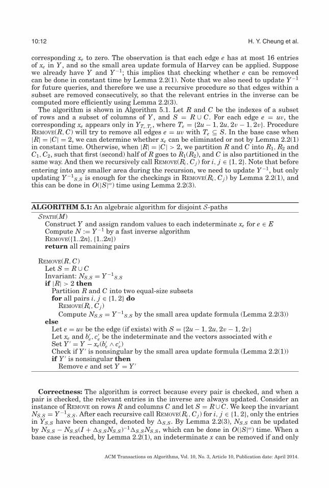
The algorithm is shown in Algorithm 5.1. Let R and C be the indexes of a subsetof rows and a subset of columns of Y , and S = R ∪ C. For each edge e = uv, thecorresponding xe appears only in YTe,Te , where Te = {2u − 1, 2u, 2v − 1, 2v}. ProcedureREMOVE(R, C) will try to remove all edges e = uv with Te ⊆ S. In the base case when|R| = |C| = 2, we can determine whether xe can be eliminated or not by Lemma 2.2(1)in constant time. Otherwise, when |R| = |C| > 2, we partition R and C into R1, R2 andC1, C2, such that first (second) half of R goes to R1(R2), and C is also partitioned in thesame way. And then we recursively call REMOVE(Ri, C j) for i, j ∈ {1, 2}. Note that beforeentering into any smaller area during the recursion, we need to update Y −1, but onlyupdating Y −1

S,S is enough for the checkings in REMOVE(Ri, C j) by Lemma 2.2(1), andthis can be done in O(|S|ω) time using Lemma 2.2(3).

ALGORITHM 5.1: An algebraic algorithm for disjoint S-pathsSPATH(M)

Construct Y and assign random values to each indeterminate xe for e ∈ ECompute N := Y −1 by a fast inverse algorithmREMOVE({1..2n}, {1..2n})return all remaining pairs

REMOVE(R, C)Let S = R ∪ CInvariant: NS,S = Y −1

S,Sif |R| > 2 then

Partition R and C into two equal-size subsetsfor all pairs i, j ∈ {1, 2} do

REMOVE(Ri, C j)Compute NS,S = Y −1

S,S by the small area update formula (Lemma 2.2(3))else

Let e = uv be the edge (if exists) with S = {2u − 1, 2u, 2v − 1, 2v}Let xe and b′

e, c′e be the indeterminate and the vectors associated with e

Set Y ′ = Y − xe(b′e ∧ c′

e)Check if Y ′ is nonsingular by the small area update formula (Lemma 2.2(1))if Y ′ is nonsingular then

Remove e and set Y = Y ′

Correctness: The algorithm is correct because every pair is checked, and when apair is checked, the relevant entries in the inverse are always updated. Consider aninstance of REMOVE on rows R and columns C and let S = R∪ C. We keep the invariantNS,S = Y −1

S,S. After each recursive call REMOVE(Ri, C j) for i, j ∈ {1, 2}, only the entriesin YS,S have been changed, denoted by �S,S. By Lemma 2.2(3), NS,S can be updatedby NS,S − NS,S(I + �S,S NS,S)−1�S,S NS,S, which can be done in O(|S|ω) time. When abase case is reached, by Lemma 2.2(1), an indeterminate x can be removed if and only



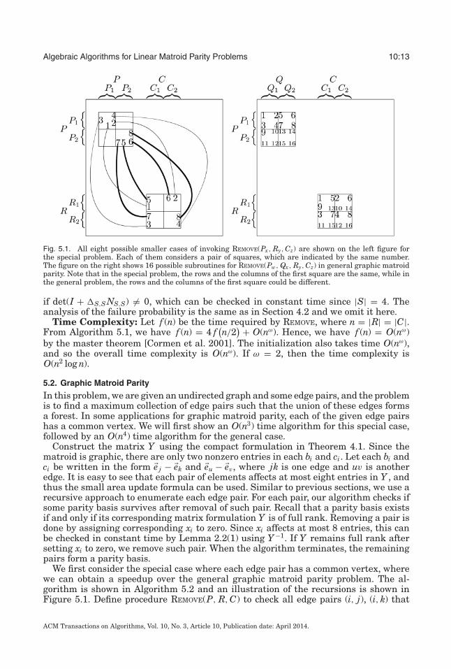
Fig. 5.1. All eight possible smaller cases of invoking REMOVE(Px, Ry, Cz) are shown on the left figure forthe special problem. Each of them considers a pair of squares, which are indicated by the same number.The figure on the right shows 16 possible subroutines for REMOVE(Pw, Qx, Ry, Cz) in general graphic matroidparity. Note that in the special problem, the rows and the columns of the first square are the same, while inthe general problem, the rows and the columns of the first square could be different.

if det(I + �S,S NS,S) �= 0, which can be checked in constant time since |S| = 4. Theanalysis of the failure probability is the same as in Section 4.2 and we omit it here.

Time Complexity: Let f (n) be the time required by REMOVE, where n = |R| = |C|.From Algorithm 5.1, we have f (n) = 4 f

(n/2

) + O(nω). Hence, we have f (n) = O(nω)by the master theorem [Cormen et al. 2001]. The initialization also takes time O(nω),and so the overall time complexity is O(nω). If ω = 2, then the time complexity isO(n2 log n).

5.2. Graphic Matroid Parity

In this problem, we are given an undirected graph and some edge pairs, and the problemis to find a maximum collection of edge pairs such that the union of these edges formsa forest. In some applications for graphic matroid parity, each of the given edge pairshas a common vertex. We will first show an O(n3) time algorithm for this special case,followed by an O(n4) time algorithm for the general case.

Construct the matrix Y using the compact formulation in Theorem 4.1. Since thematroid is graphic, there are only two nonzero entries in each bi and ci. Let each bi andci be written in the form �e j − �ek and �eu − �ev, where jk is one edge and uv is anotheredge. It is easy to see that each pair of elements affects at most eight entries in Y , andthus the small area update formula can be used. Similar to previous sections, we use arecursive approach to enumerate each edge pair. For each pair, our algorithm checks ifsome parity basis survives after removal of such pair. Recall that a parity basis existsif and only if its corresponding matrix formulation Y is of full rank. Removing a pair isdone by assigning corresponding xi to zero. Since xi affects at most 8 entries, this canbe checked in constant time by Lemma 2.2(1) using Y −1. If Y remains full rank aftersetting xi to zero, we remove such pair. When the algorithm terminates, the remainingpairs form a parity basis.

We first consider the special case where each edge pair has a common vertex, wherewe can obtain a speedup over the general graphic matroid parity problem. The al-gorithm is shown in Algorithm 5.2 and an illustration of the recursions is shown inFigure 5.1. Define procedure REMOVE(P, R, C) to check all edge pairs (i, j), (i, k) that



have i ∈ P, j ∈ R, and k ∈ C. Consider the base case where |P| = |R| = |C| = 1. Weneed to determine whether pair (i, j), (i, k) (i ∈ P, j ∈ R, k ∈ C) can be removed. Sinceremoval of such pair will only affect entries in YS,S where S = P ∪ R ∪ C, a decisioncan be made using Lemma 2.2(1) in constant time using Y −1

S,S.

ALGORITHM 5.2: An algebraic algorithm for graphic matroid parity, when each edgepair has a common vertex.

GRAPHICPARITY(M)Construct Y and assign random values to indeterminates xiN := Y −1

REMOVE({1..n}, {1..n}, {1..n})return all remaining pairs

REMOVE(P, R, C)Let S = P ∪ R ∪ CInvariant: NS,S = Y −1

S,Sif |P| = |R| = |C| = 1 then

Let i ∈ P, j ∈ R, k ∈ CLet x, b, c be the indeterminate and the vectors associated with edge pair (i, j)and (i, k) (if exists)Y ′ = Y − x(b ∧ c)Check if Y ′ is nonsingular by the small area update formula (Lemma 2.2(1))if Y ′ is nonsingular then

Remove this edge pair and set Y = Y ′else

Partition P, R, and C into two equal-size subsetsfor all tuples i, j, k ∈ {1, 2} do

REMOVE(Pi, Rj, Ck)Compute NS,S = Y −1

S,S using the small area update formula (Lemma 2.2(3))

The algorithm starts with REMOVE(V, V, V ), V = {1..n}, which will check all edgepairs. The procedure simply calls recursions when it does not reach its base casesyet. For any set T , define its first (second) half by T1 (T2). Then the procedure can beimplemented by recursive call to REMOVE(Px, Ry, Cz) for all x, y, z ∈ {1, 2}; see Figure 5.1.Since inverse of Y is required to decide if a pair can be removed, Y −1

S,S (S = P ∪ R∪C)is recomputed before each recursive call using Lemma 2.2(3), as in the algorithm forthe S-path problem.

Now we analyze the time complexity of this algorithm. Any changes done byREMOVE(P, R, C) are made to YS,S, where S = P ∪ R ∪ C. So, similar to that in theS-path problem, updating Y −1

S,S using Lemma 2.2(3) takes O(|S|ω) time. Let f (n) betime required by REMOVE, where n = |P| = |R| = |C|. We have f (n) = 8 f (n/2) + O(nω).By the master theorem [Cormen et al. 2001], if fast matrix multiplication is used,this algorithm has overall time complexity O(n3); otherwise, its time complexity isO(n3 log n) time. The analysis of the failure probability is the same as in Section 4.2and we omit it here.

For the general case where edge pairs are in the form (i, k) and ( j, l), our algorithmis very similar but the procedure is now defined as REMOVE(P, Q, R, C), which checksall pairs in the form i ∈ P, j ∈ Q, k ∈ R, and l ∈ C. Hence, we now require 16 recursioncalls of REMOVE(Pw, Qx, Ry, Cz), where w, x, y, z ∈ {1, 2}; see Figure 5.1. This gives anO(n4) time algorithm by the master theorem.



5.3. Colorful Spanning Tree

Given a connected undirected multigraph G = (V, E), where each edge is colored byone of the k colors, the colorful spanning tree problem [Schrijver 2003] is to determineif there is a spanning tree T in G such that each edge in T has a distinct color. Letn = |V | and m = |E|.

The distinct color constraint can be modeled by a partition matroid M1 = (E, I1),where I1 = {I : edges in I that contain at most one edge from each color}. The treeconstraint can be captured by a graphic matroid M2 = (E, I2), where I2 = {I :edges in I form an acyclic subgraph}. Thus, a matroid intersection (see Section 3.4 fordefinition) of M1 and M2 gives a maximum size acyclic colorful subgraph of G. In par-ticular, when k = n − 1 and G is connected, a common basis of the two matroids is acolorful spanning tree of G. Recall that a partition matroid can be represented by alinear matroid with exactly one nonzero entry in each column. This simpler structurecan be used to obtain a faster algorithm.

5.3.1. Matrix Formulation. Using the matrix formulation and the algebraic frameworkfrom Harvey [2009], there is an algebraic algorithm in solving the colorful spanningtree problem. Note that Harvey used a “sparse” formulation and his algorithm runs inO(mnω−1) time. A similar “compact” formulation for the matroid parity problem is alsoknown. We include its proof here for completeness.

THEOREM 5.2. Let M1 and M2 be linear matroids with the same ground set. LetA = (a1 a2 · · · am) be an r × m matrix whose columns represent M1 and B = (b1 b2 · · · bm)be an r × m matrix whose columns represent M2, where ai and bi are column vectors. Letmatrix

Y =m∑

i=1

xi(aibT

i

)be an r × r matrix where xi is a distinct indeterminate for 1 ≤ i ≤ m. Then the twomatroids have a common independent set of size rank(Y ).

PROOF. Harvey [2008] showed that the matrix formulation for matroid intersectionof M1 and M2 is given by

Z =(

O ABT T

),

where T is an m× m matrix with nonzero distinct indeterminates at the diagonal, thatis, Ti,i = ti. He showed that

rank(Z) = m+ λ,

where λ is the maximum cardinality of the intersection to M1 and M2.Perform Gaussian elimination in Z; by eliminating A using T , we have

rank(Z) = rank(AT −1 BT ) + m,

and we have to show AT −1 BT = ∑mi=1 xi(aibT

i ) = Y .

AT −1 BT = (a1 · · · am)T −1(b1 · · · bm)T

=(

1t1

a1 · · · 1tn

am

)(b1 · · · bm)T

=m∑

i=1

xi(aibT

i

),

where xi = 1ti.



5.3.2. An O(n3) Algorithm. The idea of the algorithm is to examine each edge e one by oneand see if any common basis (that is a colorful spanning tree) remains after removal ofthis edge. We construct Y as described in Theorem 5.2. Let the matrix representing M1be (a1 a2 · · · am) and the matrix representing M2 be (b1 b2 · · · bm). Note that both ai and bihave size n× 1. For an edge ei = (u, v) that has color c, we have ai = �ec and bi = �eu − �ev.Then xi will only appear in Yc,u and Yc,v. Let Y ′ be the new matrix with xi assigned tozero, which is equivalent to remove edge ei. Let S = {c, u, v}; Y ′ is identical to Y exceptY ′

S,S. Recall that we can remove edge ei if the rank of Y ′ remains the same. If so, wesimply remove that edge and update Y −1. After checking all edges, a common basisremains. If the size of the common basis is n − 1, then it is a colorful spanning tree.

One technical point is that we require Y to have full rank before the checking starts.In our problem, the originally constructed matrix Y is never full rank. So we needanother matrix that gives the same result as Y while having full rank. We will de-scribe in Section 5.3.3 how to find such a matrix using similar technique described inSection 6.5. Henceforth we assume that Y is of full rank.

The algorithm is shown in Algorithm 5.3, which is similar to that for the graphicmatroid parity problem. Let R be a subset of rows of Y , and C and C ′ be a subsetof columns of Y . Define procedure REMOVE(R, C, C ′), which tries to remove edges con-necting u and v having color c that have c ∈ R, u ∈ C, v ∈ C ′. REMOVE(R, C, C ′) has|R| = |C| = |C ′| = 1 as the base case, where we have to determine that a particularedge (u, v) having color c can be removed (c ∈ R, u ∈ C, v ∈ C ′). This can be done inconstant time using Lemma 2.2(1) because removing such edge only affects two entriesin Y . In other cases, R, C and C ′ are partitioned into R1, R2, C1, C2, and C ′

1, C ′2. All

eight smaller cases REMOVE(Ri, C j, C ′k) will be called, where i, j, k ∈ {1, 2}. After any

recursive call, Y −1 is updated using Lemma 2.2(3). Let S = R ∪ C ∪ C ′; any instanceof REMOVE(R, C, C ′) triggers updates to YS,S. The updating process takes only O(|S|ω)time.

ALGORITHM 5.3: An algorithm to compute colorful spanning treeCOLORFULSPANNINGTREE(M1, M2)

Construct Y and assign random values to indeterminates xiCompute N := Y −1 by fast inverseREMOVE({1..n}, {1..n}, {1..n})return all remaining pairs

REMOVE(R, C, C ′)Let S = R ∪ C ∪ C ′Invariant: NS,S = Y −1

S,Sif |R| = 1 then

Let x, b, c be the indeterminate and the vectors associated with the edge in YS,S(if exists)Y ′ = Y − x(b ∧ c)Check if Y ′ is nonsingular using the small area update formula (Lemma 2.2(1))if Y ′ is nonsingular then

Set x = 0 and Y = Y ′else

Partition R, C and C ′ into two equal-size subsetsfor all tuples i, j, k ∈ {1, 2} do

REMOVE(Ri, C j, C ′k)

Compute NS,S = Y −1S,S using the small area update formula (Lemma 2.2(3))



Time Complexity: Let f (n) be the time required by REMOVE, where n = |R| = |C| =|C ′|. We have f (n) = 8 f (n/2) + O(nω). Hence, f (n) = O(n3) by the master theorem. Asa result, the algorithm has time complexity O(n3). If fast matrix multiplication is notused, then the algorithm has time complexity O(n3 log n) again by the master theorem.

5.3.3. Maximum Cardinality Matroid Intersection. Construct Y as in Theorem 5.2. Letrank(Y ) = k. Then the largest intersection of the two matroids will be k. Since Yis not of full rank, we compute a largest rank submatrix of Y . Let Y ′ = YR,C be suchmatrix where |R| = |C| = k. Let N1 and N2 be linear matroids constructed by remov-ing row set R from M1 and row set C from M2, respectively. Observe that the matrixformulation for intersection of N1 and N2 is

∑mi=1 xi(AR,i BT

C,i), which is exactly Y ′. Anindependent set in N1 is also independent in M1, and this is also true for N2 and M2.Since Y ′ is of full rank, we can simply compute a common base of N1 and N2. Theresult will have size k, and it is a maximum cardinality intersection of M1 and M2.The maximum rank submatrix Y ′ can be computed in O(nω) time using the algorithmsuggested by Harvey (Appendix A in Harvey [2008]).

6. A FASTER LINEAR MATROID PARITY ALGORITHM

In this section, we present an O(mrω−1)-time randomized algorithm for the linearmatroid parity problem. We first consider the problem of determining whether M hasa parity basis and show how to reduce the general problem into it in Section 6.5. Thealgorithm is very similar to the algebraic algorithm for linear matroid intersection byHarvey [2009]. The general idea is to build a parity basis incrementally. A subset ofpairs is called growable if it is a subset of some parity basis. Starting from the emptysolution, at any step of the algorithm we try to add a pair to the current solution sothat the resulting subset is still growable, and the algorithm stops when a parity basisis found.

6.1. Preliminaries

Suppose A, B, C, and D are respectively p × p, p × q, q × p, and q × q matrices, and Ais invertible. Let M be a (p + q) × (p + q) matrix so that

M =(

A BC D

);

then D − C A−1 B is called the Schur complement of block A.

THEOREM 6.1 (SCHUR’S FORMULA [ZHANG 2005] (THM 1.1)). Let A, B, C, D, and M bematrices defined earlier. Then det(M) = det(A) × det(D − C A−1 B).

LEMMA 6.2. If A is nonsingular and its Schur complement S = D − C A−1 B is alsononsingular, then

M−1 =(

A−1 + A−1 BS−1C A−1 −A−1 BS−1

−S−1C A−1 S−1

).

In particular, if we have a matrix Z in the form

Z =(

0 Q1Q2 T

)and T is nonsingular, denote Y as the Schur complement of T in Z. We have Y =−Q1T −1 Q2. Then, by Lemma 6.2, if Y is nonsingular, we can calculate Z−1 as follows:

Z−1 =(

Y −1 −Y −1 Q1T −1

−T −1 Q2Y −1 T −1 + T −1 Q2Y −1 Q1T −1

). (6.1)



6.2. Matrix Formulation

We use the matrix formulation of Geelen and Iwata [2005]. Define

Z :=(

0 M−MT T

)as in Theorem 4.2. Then we have νM = r/2 if and only if Z is of full rank. To determinewhether a subset J of pairs is growable, we define Z(J) to be the matrix that has ti = 0for all pairs i in J. We define νM/J to be the optimal value of the linear matroid parityproblem of M/J, which is the contraction of M by J as stated in Section 3. Informally,the linear matroid parity problem of M/J corresponds to the linear matroid parityproblem of M when the pairs in J are picked. In the following, we will show, followingfrom the Geelen-Iwata formula, that J is growable if and only if Z(J) is of full rank.

COROLLARY 6.3. For any independent parity set J, rank(Z(J)) = 2νM/J + 2m+ |J|.PROOF. In the following, let R be the set of rows of M and V be the set of columns of

M (i.e., |V | = 2m). Note that Z(J) is in the following form:

⎛⎜⎝

R J V \ J

R MR,J MR,V \J

J (−MT )J,R

V \ J (−MT )V \J,R TV \J,V \J

⎞⎟⎠

︸︷︷︸Z(J)

=

⎛⎜⎝

R J V \ J

R MR,J MR,V \J

J (−MT )J,R

V \ J (−MT )V \J,R

⎞⎟⎠

︸︷︷︸P

+

⎛⎜⎝

R J V \ J

RJV \ J TV \J,V \J

⎞⎟⎠

︸︷︷︸Q

.

It is known ([Murota 2009], Theorem 7.3.22) that for a mixed skew-symmetric matrix,we have

rank(Z(J)) = maxA⊆S

{rank(PA,A) + rank(QS\A,S\A)}, (6.2)

where S = R ∪ V is the column set and row set for Z(J). Consider a set A thatmaximizes rank(Z(J)); then A must be in the form R ∪ A′ where J ⊆ A′ ⊆ V .

Recall that a set is a parity set if every pair is either contained in it or disjoint fromit. We can assume that A′ is a parity set. If A′ is not, consider parity set B′ such thatA′ ⊆ B′ and B′ has the smallest size. Let B = R ∪ B′. We have rank(PA,A) ≤ rank(PB,B)and rank(QS\A,S\A) = rank(QS\B,S\B), where the equality follows from the structureof T .

As M and −MT occupy disjoint rows and columns of P, rank(PA,A) = rank(MR,A′) +rank((−MT )A′,R) = 2 rank(MR,A′) as M is skew symmetric. We also haverank(QS\A,S\A) = |S \ A| = |V \ A′| = |V | − |A′|. Thus,

rank(Z(J)) = maxA′⊆V

{2 rank(MR,A′) + |V | − |A′|}.



Write A′ = I ∪ J, where I ∩ J = ∅ and I is a parity set. By the rank function rM/J ofthe matroid M/J, we have rM/J(A′ \ J) = rM(A′) − rM(J). Hence,

rank(Z(J)) = maxI⊆V \J

{2(rM/J(I) + |J|) + |V | − (|I| + |J|)}= max

I⊆V \J{2rM/J(I) − |I|} + |V | + |J|. (6.3)

Observe that a maximizer I′ of Equation (6.3) must be an independent parity set (sorM/J(I′) = |I′|); otherwise, an independent set K ⊂ I′ such that rM/J(K) = rM/J(I′) and|K| < |I′| gives a larger value for Equation (6.3). So a maximizer I′ of Equation (6.3)would maximize rM/J(I), which implies that I′ is indeed a maximum cardinality parityset of M/J. The result follows since 2νM/J = |I′| = rM/J(I′).

THEOREM 6.4. For any independent parity set J, Z(J) is nonsingular if and only if Jis growable.

PROOF. If Z(J) is nonsingular, by Corollary 6.3, we have

rank(Z(J)) = 2νM/J + |V | + |J|2m+ r = 2νM/J + 2m+ |J|

r = 2νM/J + |J|.Hence, J is growable.

6.3. An O(mω) Algorithm

The algorithm here maintains a growable set J, starting with J = ∅. To check whethera pair i can be added to J to form a growable set, we test whether Z(J ∪ {2i − 1, 2i})is of full rank. Observe that Z(J ∪ {2i − 1, 2i}) is obtained from Z(J) by a small areaupdate, and so Lemma 2.2 can be used to check whether Z(J ∪ {2i − 1, 2i}) is of fullrank more efficiently. Pseudocode of the algorithm is shown in Algorithm 6.1.

First we show how to check whether a pair can be included in J to form a largergrowable set.

CLAIM 6.1. Let N = Z(J)−1, ni = N2i−1,2i , and J′ = J ∪ {2i − 1, 2i}. Then J′ is agrowable set if and only if tini + 1 �= 0.

PROOF. By Theorem 6.4, J′ is growable if and only if Z(J′) is nonsingular. ByLemma 2.2(1), this is true if and only if the following expression is nonzero:

det((

1 00 1

)−

(0 ti

−ti 0

)·(

0 ni−ni 0

))= det

(tini + 1 0

0 tini + 1

),

Thus, Z(J′) is nonsingular if and only if (tini + 1)2 �= 0, which is equivalent to tini + 1 �=0.

Correctness: At the time MATROIDPARITY calls BUILDPARITY, the invariant N = Z(J)−1

obviously holds, and so as the first recursive call to BUILDPARITY. Regardless of thechanges made in the first recursive call, Z(J ∪ J1)−1 is recomputed so the invariant isalso satisfied with the second recursive call. Note that S is partitioned in such a waythat its first half goes to S1 and the remaining goes to S2, so both S1 and S2 must be aparity set.

In the algorithm, every element of M is considered. By Claim 6.5, Z(J) is alwaysnonsingular. Hence, by Theorem 6.4, this implies that J is always a growable set.



ALGORITHM 6.1: An O(mω)-time algebraic algorithm for linear matroid parityMATROIDPARITY(M)

Construct Z and assign random values to indeterminates tiCompute N := Z−1 by fast matrix inversereturn BUILDPARITY(S, N,∅)

BUILDPARITY(S,N,J)Invariant 1: J is a growable setInvariant 2: N = Z(J)−1

S,Sif |S| = 2 then

Let S = {2i − 1, 2i}if 1 + ti N2i−1,2i �= 0 then

return {2i − 1, 2i}else

return ∅else

Partition S into two equal-size subsetsJ1 := BUILDPARITY(S1, NS1,S1 , J)Compute M := Z(J ∪ J1)−1

S2,S2 using Claim 6.2J2 := BUILDPARITY(S2, M, J ∪ J1)return J1 ∪ J2

Time complexity: The following claim shows how to compute M := Z(J ∪ J1)−1S2,S2

efficiently.

CLAIM 6.2. Let J′ = J ∪ J1, J1 ⊆ S. Using N = Z(J)−1S,S, computing Z(J′)−1

S,S canbe done in O(|S|ω) time.

PROOF. Since Z(J′) is identical to Z(J) except Z(J′)J1,J1 = 0, since Z(J)−1R,C = NR,C ,

by Lemma 2.2(3),

Z(J′)−1S,S = NS,S − NS,J1 (I + (−Z(J)J1,J1 )NJ1,J1 )

−1(−Z(J)J1,J1 )NJ1,S

= NS,S + NS,J1 (I − ZJ1,J1 NJ1,J1 )−1 ZJ1,J1 NJ1,S.

Note the last equality holds because Z(J)J1,J1 = ZJ1,J1 . At any time during the com-putation, matrices involved have size at most |S| × |S|. Hence, computing Z(J′)−1

S,Stakes O(|S|ω) time.

Since Z has dimension (2m + r) × (2m + r), initial computation of Z−1S,S takes

O((2m+r)ω) = O(mω) time. Let f (m) be the time required by BUILDPARITY with |S| = 2m;then

f (m) = 2 · f (m/2) + O(mω),

which implies f (n) = O(mω) by the master theorem.

6.4. An O(mrω−1) Algorithm

The previous algorithm works for matroids with large rank. In this section, we presentan algorithm with better time complexity when rank is small. The idea behind this isto break the ground set S into a number of smaller pieces. In this way, the inverse ofthese matrices to be computed will have a smaller size.

The matrix Y = MT −1MT will allow us to compute submatrices of Z(J)−1 efficientlyusing Equation 6.1. We will assume Y −1 exists; otherwise, if Y has no inverse, we can



ALGORITHM 6.2: An O(mrω−1)-time algebraic algorithm for linear matroid parityMATROIDPARITY(M)

Construct Z and assign random values to indeterminates tiCompute Y := MT −1MT using Claim 6.3Partition S into m/r subsets each with size rJ := ∅for i = 1 to m/r do

Compute N := Z(J)−1Si ,Si using Claim 6.5

J′ := BUILDPARITY(Si, N, J)J := J ∪ J′

return J

conclude that Z has no inverse by Theorem 6.1 and thus there is no parity basis. In thefollowing, we will show how to compute Y efficiently, and then show how to computeZ(J)−1

Si ,Si efficiently.

CLAIM 6.3. Computation of Y := MT −1MT can be done in O(mrω−1) time.

PROOF. First we show that MT −1R,C can be computed in O(RC) time. Recall that T is

a skew-symmetric matrix, having exactly one entry in each row and column. Moreover,the positions of the nonzero entries in T are just one row above or below the diagonalof T . It is thus easy to compute T −1. If Ti, j is zero, then T −1

i, j is also zero. Otherwise,T −1

i, j = −1/Ti, j . As a result, T −1 is also skew symmetric and shares the same specialstructure of T . Therefore, any entry of MT −1 can be computed in O(1) time. Hence,MT −1

R,C takes O(RC) to compute.Now we are going to show that MT −1MT can be computed in O(mrω−1) time. Since

M has size r × m, MT −1 can be computed in O(mr) time. To compute product of MT −1

(size r × m) and MT (size m× r), we can break each of them into m/r matrices each ofsize r × r, so computation of their products takes O(mrω−1).

Next we show how to compute Z(J)−1Si ,Si efficiently using Y and Y −1.

CLAIM 6.4. Given the matrix Y = MT −1MT , for any A, B ⊆ S with |A|, |B| ≤ r, Z−1A,B

can be computed in O(rω) time.

PROOF. By Equation 6.1,

Z−1S,S = T −1 − T −1MT Y −1MT −1.

Hence, for any A, B ⊆ S,

Z−1A,B = T −1

A,B − (T −1MT )A,∗Y −1(MT −1)∗,B.

Both (T −1MT )A,∗ and (MT −1)∗,B have size r × r and can be computed in O(r2) time byClaim 6.3. Thus, the whole computation takes O(rω) time.

CLAIM 6.5. In each loop iteration, the matrix Z(J)−1Si ,Si can be computed in O(rω)

time.

PROOF. Since Z(J) is identical to Z except Z(J)J,J = 0, by using Lemma 2.2(3) withMSi ,Si − MSi ,Si = −Z(J)J,J , we have

Z(J)−1Si ,Si = Z−1

Si ,Si + Z−1Si ,J(I − ZJ,J Z−1

J,J)−1 ZJ,J Z−1J,Si .

All the submatrices Z−1Si ,Si , Z−1

Si ,J, Z−1J,J, and Z−1

J,Si can be computed in O(rω) byClaim 6.4. Thus, the whole computation can be done in O(rω) time.



Since |Si| = r, each call to BUILDPARITY takes O(rω) time. Hence, the overall timecomplexity of Algorithm 6.2 is O(m/r · rω) = O(mrω−1).

6.5. Maximum Cardinality Matroid Parity

The algorithms in previous sections can only produce a parity basis if one exists. Ifthere is no parity basis, these algorithms are only able to report so. In this section, wepresent how to find the maximum number of pairs that are independent. We are goingto show an O(rω) time reduction, which reduces a maximum cardinality matroid parityproblem to a problem of computing parity basis. Hence, algorithms in previous sectionscan be applied.

The idea here is to find a maximum rank submatrix of the matrix formulation formatroid parity. Such a submatrix is of full rank and corresponds to a new instance ofthat matroid parity problem, which has a parity basis.

Let Y be a matrix formulation for the parity problem constructed as in Theorem 4.1.Let r′ be the rank of Y . We first find a maximum rank submatrix YR,C of Y where|R| = |C| = r′. This can be done in O(rω) time using a variant of the LUP decompositionalgorithm by Harvey (Appendix A of Harvey [2008]). Since Y is a skew-symmetric ma-trix, YR,R is also a maximum rank submatrix of Y (see Murota [2009] Proposition 7.3.6).

The matrix YR,R can be interpreted as a matrix formulation for a new matroid parityinstance. Such an instance contains all the original given pairs but only contains rowsindexed by R. Then

m∑i=1

xi(biR ∧ ciR) = YR,R,

where biR denotes the vector containing entries of bi index by R. Since YR,R is of fullrank, such a new instance of matroid parity has a parity basis.

The column pairs that are independent in the new instance are also independent inthe original instance. Hence, a parity basis of this new instance corresponds to a parityset of the original instance. In addition, this new instance for matroid parity can besolved using any algorithm presented.

For Algorithm 6.2 to keep the same time complexity O(mrω−1), this reduction hasto be done under the same time. However, naive construction of Y takes O(mr2) time.Indeed, Y = MT −1MT , which can be computed in O(mrω−1) time by Claim 6.3. Theproof for Y = MT −1MT , where xi = −1/ti (xi and ti are indeterminates in Y and T ,respectively), is similar to the one of Theorem 5.2; we refer the reader to Murota [2009,p. 445] for the sketch of the proof.

7. WEIGHTED LINEAR MATROID PARITY

In the weighted matroid parity problem, each pair i is assigned a weight wi, and theobjective is to find a parity basis with maximum weight. Camerini et al. [1992] gavea compact matrix formulation to find the parity basis with maximum weight p. Thematrix formulation Y ∗ is almost the same as the formulation Y for the unweightedcase in Theorem 4.1. The only exception is that all indeterminates xi are now replacedby xi ywi .

THEOREM 7.1 (CAMERINI ET AL. [1992]). Let

Y ∗ =m∑

i=1

xi(bi ∧ ci)ywi ,

where the pairs {(bi, ci)} compose M, and xi and y are indeterminates. Then



(1) each nonzero term of pf Y ∗ corresponds to a parity basis of M;(2) the degree of y in each term is the weight of the corresponding parity basis.

Here pf Y denotes the Pfaffian (see Murota [2009]) of a skew-symmetric matrix Y .Each term of pf Y corresponds to a partition of the row set of Y into pairs. For an evendimension skew-symmetric matrix Y , it is known that det Y = (pf Y )2 (see Murota[2009]).

Since removing each pair is equivalent to assigning xi = 0, the aforementionedtheorem gives an algorithm for the weighted problem similar to Algorithm 4.1, butwe need to make sure that some parity basis with maximum weight is preserved.Therefore, we have to calculate pf Y ∗ to see if a term containing yp still remains. Itcan be achieved by finding det(Y ∗) and looking for a term that contains y2p. How-ever, calculating its determinant may not be easy. Define W = maxi{wi}. Cameriniet al. [1992] proposed an O(m2r2 + Wmr4) algorithm in finding the parity basis withmaximum weight. Sankowski [2006] used the following theorem of Storjohann [2003]to design a faster pseudo-polynomial algorithm for the weighted bipartite matchingproblem.

THEOREM 7.2 (STORJOHANN [2003]). Let A ∈ F[x]n×n be a polynomial matrix of degreed and b ∈ F[x]n×1 be a polynomial vector of the same degree, then

—determinant det(A),—rational system solution A−1b,

can be computed in O(nωd) operations in K, with high probability.

Now we can apply Theorem 7.2 to get the determinant det(Y ∗). By choosing a largeenough field F, we can check if removing each pair i (by assigning xi = 0) would affectthe parity basis with maximum weight, with high probability. If the degree of det(Y ∗)does not drop after removal of a pair, then it can be removed. And removal of a pair canbe simply done by a rank-2 update to Y ∗ in O(r2) time. Each time the checking can bedone in O(Wrω) time by Theorem 7.2, which dominates the updating time. CalculatingY ∗ at the beginning takes O(mr2) time. Hence, we can find a parity basis with themaximum weight in O(Wmrω) time. The pseudocode of the algorithm can be found inAlgorithm 7.1.

ALGORITHM 7.1: An algebraic algorithm for weighted linear matroid parityMAXWEIGHTPARITY(M)

Construct Y ∗ and assign random values to indeterminates xiJ := {b1, c1, . . . bm, cm}for i = 1 to m do

Y := Y ∗ − xi(bi ∧ ci)ywi

if degree of det(Y ) equals that of det(Y ∗) thenY ∗ := YJ := J − {bi, ci}

return J

Finally, we describe how to obtain a randomized FPTAS using the pseudo-polynomialalgorithm by standard scaling technique [Promel and Steger 1997]. Here we assumeevery column pair is contained in some parity basis. This assumption can be satisfiedby checking the rank of corresponding Z(J) as in Theorem 6.4. If Z(J) is not full rank,we discard the corresponding column pair.



The idea is to scale the weight of each pair down and solve the new instance us-ing Algorithm 7.1. Given ε > 0, let K = εW/r. For each pair i, scale its weight tow∗

i = �wi/K�. Solve the new instance using Algorithm 7.1. This takes O(�W/K� mrω) =O(mrω+1/ε) time.

We will show that the result of the scaled instance is an (1 − ε)-approximation of theoriginal instance. Let J and O be the pairs returned by the previous algorithm andthe optimal pairs, respectively. Also denote original (scaled) weight of a set S by w(S)(w∗(S)). We have w(O) − Kw∗(O) ≤ rK because for each pair in O, at most weight withvalue K is lost, and there are at most r/2 pairs chosen. Then

w(J) ≥ K · w∗(J) ≥ K · w∗(O) ≥ w(O) − rK = w(O) − εW ≥ (1 − ε) · w(O).

8. CONCLUDING REMARKS

A recent work [Cheung et al. 2013] shows that the O(mrω−1)-time algorithm for thelinear matroid parity problem can be improved to O(mr + m(νM)ω−1) time. In addition,all graph algorithms presented here can be improved similar to the way algebraic graphmatching algorithms are improved in the same paper by Cheung et al.

ACKNOWLEDGMENT

We thank Nick Harvey for helpful discussions on this topic.

REFERENCES

M. A. Babenko. 2010. A fast algorithm for the path 2-packing problem. Theory of Computing Systems 46, 1(2010), 59–79.

P. Berman, M. Furer, and A. Zelikovsky. 2006. Applications of the linear matroid parity algorithm to approx-imating steiner trees. In Proceedings of the 1st International Computer Science Symposium in Russia(CSR). 70–79.

A. Bouchet and W. H. Cunningham. 1995. Delta-matroids, jump systems, and bisubmodular polyhedra. SIAMJournal on Discrete Mathematics 8, 1 (1995), 17–32.

J. R. Bunch and J. E. Hopcroft. 1974. Triangular factorization and inversion by fast matrix multiplication.Math. Comp. 28, 125 (1974), 231–236.

G. Calinescu, C. G. Fernandes, U. Finkler, and H. Karloff. 1998. A better approximation algorithm for findingplanar subgraphs. Journal of Algorithms 27, 2 (1998), 269–302.

P. M. Camerini, G. Galbiati, and F. Maffioli. 1992. Random pseudo-polynomial algorithms for exact matroidproblems. Journal of Algorithms 13, 2 (1992), 258–273.

H. Y. Cheung, T. C. Kwok, and L. C. Lau. 2013. Fast matrix rank algorithms and applications. Journal of theACM 60, 5 (Oct. 2013), 1–25.

M. Chudnovsky, W. H. Cunningham, and J. Geelen. 2008. An algorithm for packing non-zero A-paths ingroup-labelled graphs. Combinatorica 28, 2 (2008), 145–161.

T. H. Cormen, C. E. Leiserson, R. L. Rivest, and C. Stein. 2001. Introduction to Algorithms. MIT Press.W. H. Cunningham and J. F. Geelen. 1997. The optimal path-matching problem. Combinatorica 17, 3 (1997),

315–337.M. L. Furst, J. L. Gross, and L. A. McGeoch. 1988. Finding a maximum-genus graph imbedding. Journal of

the ACM 35, 3 (1988), 523–534.H. N. Gabow and M. Stallmann. 1985. Efficient algorithms for graphic matroid intersection and parity. In

Proceedings of the 12th International Colloquium on Automata, Languages and Programming (ICALP).210–220.

H. N. Gabow and M. Stallmann. 1986. An augmenting path algorithm for linear matroid parity. Combina-torica 6, 2 (1986), 123–150.

H. N. Gabow and Y. Xu. 1989. Efficient algorithms for independent assignment on graphic and linearmatroids. In Proceedings of the 30th Annual Symposium on Foundations of Computer Science (FOCS).106–111.



J. Geelen and S. Iwata. 2005. Matroid matching via mixed skew-symmetric matrices. Combinatorica 25, 2(2005), 187–215.

N. J. A. Harvey. 2007. An algebraic algorithm for weighted linear matroid intersection. In Proceedings of the18th Annual ACM-SIAM Symposium on Discrete algorithms (SODA). 444–453.

N. J. A. Harvey. 2008. Matchings, Matroids and Submodular Functions. Ph.D. Dissertation. MassachusettsInstitute of Technology.

N. J. A. Harvey. 2009. Algebraic algorithms for matching and matroid problems. SIAM Journal of Computing39, 2 (2009), 679–702.

T. A. Jenkyns. 1974. Matchoids: a generalization of matchings and matroids. Ph.D. Dissertation. Universityof Waterloo.

P. M. Jensen and B. Korte. 1982. Complexity of matroid property algorithms. SIAM Journal of Computing11 (1982), 184–190.

T. Jordan. 2010. Rigid and globally rigid graphs with pinned vertices. In Fete of Combinatorics and Com-puter Science. Bolyai Society Mathematical Studies, Vol. 20. Springer Berlin Heidelberg, 151–172.http://dx.doi.org/10.1007/978-3-642-13580-4_7

E. L. Lawler. 1976. Combinatorial Optimization: Networks and Matroids. Oxford University Press.L. Lovasz. 1979. On determinants, matchings and random algorithms. In Fundamentals of Computation

Theory, Vol. 79. 565–574.L. Lovasz. 1980. Matroid matching and some applications. Journal of Combinatorial Theory, Series B 28, 2

(1980), 208–236.L. Lovasz. 1997. The membership problem in jump systems. Journal of Combinatorial Theory, Series B 70,

1 (1997), 45–66.L. Lovasz and M. D. Plummer. 1986. Matching Theory. Elsevier.W. Mader. 1978. Uber die maximalzahl kreuzungsfreier H-Wege. Archiv der Mathematik 31, 1 (1978), 387–

402.M. Mucha and P. Sankowski. 2004. Maximum matchings via gaussian elimination. In Proceedings of the

45th Annual IEEE Symposium on Foundations of Computer Science (FOCS). 248–255.K. Murota. 2009. Matrices and Matroids for Systems Analysis. Springer Verlag.H. Narayanan, H. Saran, and V. V. Vazirani. 1994. Randomized parallel algorithms for matroid union and

intersection, with applications to arborescences and edge-disjoint spanning trees. SIAM Journal ofComputing 23, 2 (1994), 387–397.

C. St. J. A Nash-Williams. 1985. Connected detachments of graphs and generalized Euler trails. Journal ofthe London Mathematical Society 2, 1 (1985), 17–29.

J. B. Orlin. 2008. A fast, simpler algorithm for the matroid parity problem. In Proceedings of the 13thInternational Conference on Integer Programming and Combinatorial Optimization (IPCO). 240–258.

J. B. Orlin and J. H. Vande Vate. 1990. Solving the linear matroid parity problem as a sequence of matroidintersection problems. Mathematical Programming: Series A and B 47, 1 (1990), 81–106.

G. Pap. 2007a. Packing non-returning A-Paths. Combinatorica 27, 2 (2007), 247–251.G. Pap. 2007b. Some new results on node-capacitated packing of A-paths. In Proceedings of the 39th Annual

ACM Symposium on Theory of Computing (STOC). 599–604.G. Pap. 2008. Packing non-returning A-paths algorithmically. Discrete Mathematics 308, 8 (2008), 1472–

1488.H. J. Promel and A. Steger. 1997. RNC-approximation algorithms for the steiner problem. In Proceed-

ings of the 14th Annual Symposium on Theoretical Aspects of Computer Science (STACS). 559–570.

P. Sankowski. 2006. Weighted bipartite matching in matrix multiplication time. In Proceedings of the 33rdInternational Colloquium on Automata, Languages and Programming (ICALP). 274–285.

A. Schrijver. 2003. Combinatorial Optimization: Polyhedra and Efficiency. Springer Verlag.A. Sebo and L. Szego. 2004. The path-packing structure of graphs. In Proceedings of the 10th Conference on

Integer Programming and Combinatorial Optimization (IPCO). 131–143.A. Storjohann. 2003. High-order lifting and integrality certification. Journal of Symbolic Computation 36,

3–4 (2003), 613–648.A. Stothers. 2010. On the complexity of matrix multiplication. Ph.D. Dissertation. University of Edinburgh.Z. Szigeti. 1998. On a min-max theorem of cacti. In Proceedings of the 6th Conference on Integer Programming

and Combinatorial Optimization (IPCO). 84–95.


http://dx.doi.org/10.1007/978-3-642-13580-4_7


Z. Szigeti. 2003. On the graphic matroid parity problem. Journal of Combinatorial Theory, Series B 88, 2(2003), 247–260.

V. Vassilevska Williams. 2012. Multiplying matrices faster than Coppersmith-Winograd. In Proceedings ofthe 44th ACM Symposium on Theory of Computing (STOC). 887–898.

M. A. Woodbury. 1950. Inverting modified matrices. Memorandum Report 42 (1950), 106.F. Zhang. 2005. The Schur Complement and Its Applications. Springer Verlag.

Received March 2011; revised July 2013; accepted December 2013


Documents

10 Algebraic Algorithms for Linear Matroid Parity Problemshoyeeche/papers/parity.pdf · 10 Algebraic Algorithms for Linear Matroid Parity Problems HO YEE CHEUNG, LAP CHI LAU, and