1

White Space Ecosystem: A Secondary NetworkOperator’s Perspective

Yuan Luo, Lin Gao, and Jianwei Huang

Abstract—The successful deployment of a TV whitespace network requires the coordination and cooperationof all involved parties (including licensees, databases, sec-ondary operators, and end-users), which form the WhiteSpace Ecosystem. In this paper, we study the white spaceecosystem from the perspective of secondary network op-erators. Specifically, we consider a competitive white spacenetwork, where multiple secondary operators compete forthe same pool of end-users. Each operator serves theattracted end-users by using either the dedicated spec-trum (pre-ordered in advance) or the shared spectrum (re-quested in real-time). The key problem for each operator isto (i) determine the order quantity of dedicated spectrum,considering the uncertainty of end-user demand, and (ii)decide the price to the end-users, considering the compe-tition of other operators. We formulate the interaction ofoperators as a non-cooperative Price-Quantity competitiongame (PQ-game), and study the existence and uniquenessof the Nash equilibrium (NE) systematically. We furthercharacterize the impacts of the operator competition on thesocial welfare and the operators’ own profits. Our resultsshow that such impacts depend largely on the operators’cost of purchasing spectrum from the database or licensee:when the cost is low, the operator competition will decreasethe social welfare and the operators’ profits; when the costis high, however, the competition will increase the socialwelfare and the operators’ profits.

I. INTRODUCTION

Dynamic spectrum sharing can effectively improvespectrum efficiency and alleviate spectrum scarcity, byallowing unlicensed users access to the licensed spec-trum opportunistically. TV white space network is one ofthe most promising commercial realizations of dynamicspectrum sharing [1], where unlicensed devices (calledwhite space devices, WSDs1) explore and exploit theunder-utilized broadcast television spectrum (called TVwhite spaces, TVWS2), usually via a third-party databasecalled geo-location database [2]. Figure 1 illustrates thedetailed spectrum access process in a TV white spacenetwork. The successful deployment of such a TV whitespace network requires the coordination and cooperationof all involved parties (including licensees, databases,

1This work is supported by the General Research Funds (ProjectNumber CUHK 412710 and CUHK 412511) established under the Uni-versity Grant Committee of the Hong Kong Special Administrative Re-gion, China. Author emails: {ly011, lgao, jwhuang}@ie.cuhk.edu.hk.

1A WSD can be either (i) a personal/portable device owned bya secondary user or (ii) an infrastructure-based device owned by asecondary (network) operator (as illustrated in Figure 1).

2For convenience, we will call TVWS as spectrum in this paper.

Geo-location(Database)

Licensees(TV, PMSE, etc)

Step 0Step 3

Step 1

Step 2 End-users(Slaves)WSD

(Master)

Figure 1: Illustration of a TV white space network. In step0, the geo-location database updates the licensee informationperiodically. In step 1, the WSD reports its location to thedatabase (via Internet). In step 2, the database computes andreturns the available spectrum. In step 3, the WSD serves end-users using the granted spectrum.

secondary users and operators, and end-users), whichform the White Space Ecosystem [3].

Most of the existing studies on TV white spacenetwork focused on the technical aspects of networkdeployment [4]–[6]. Some recent results considered theeconomic issues in operating a white space network, e.g.,spectrum reserving [7] and pricing [8]. However, all ofthe above works did not consider the competition amongsecondary network operators, which is an important issueof the white space ecosystem. This is because the TVwhite space will be used by secondary operators in ashared basis, which is quite different from the exclusivespectrum usage model of the current cellular networks.Because of this, when a commercial entity (such as anexisting cellular operator) wants to enter the TV whitespace network, it needs to understand the complicatedinteractions between the secondary operators in this newnetwork, and whether it is profitable to provide servicesto secondary end-users. Without a good understandingof this issue, it is difficult to envision strong commer-cializations of the new technologies.

In this paper, we study the white space ecosystemfrom the perspective of secondary network operators.In particular, we consider such a white space network,where multiple secondary operators (each operating oneor multiple infrastructure-based WSDs) compete for thesame pool of end-users. Each operator may only attracta subset of the end-users, and it serves the attractedend-users by using either the dedicated spectrum or theshared spectrum. More precisely, a dedicated spectrum isexclusively used by one WSD at a particular location andtime (and thus without co-channel interference), while ashared spectrum is shared by many nearby WSDs con-currently using certain multiple access techniques (andthus with co-channel interference). According to thesuggestions of FCC [1] and Ofcom [2], the dedicated

spectrum must be reserved (pre-ordered) in advance,while the shared spectrum can be requested in real-time. It is notable that the demand of end-users (to aparticular operator) is a random variable, due to theuncertainties of end-users’ service requirements as wellas their mobilities. In such a competitive network underdemand uncertainty, each operator needs to decide thefollowing two questions:1) What is the optimal order quantity of dedicated spec-

trum, considering the uncertainty of demand?2) What is the optimal prices of both dedicated spec-

trum and shared spectrum to the end-users, consid-ering the competition of other operators?

Each operator chooses the ordering and pricing strate-gies to optimize its own profit, taking into considera-tion all other operators’ ordering and pricing choices.Therefore, the interactions between operators can bemodeled as a non-cooperative game, which we call thePrice-Quantity competition game (PQ-game). We studythe existence and uniqueness of the Nash equilibrium(NE) systematically. We further compare the NE withthose arising in the monopoly scenario (where eachoperator faces a separate pool of end-users), in order tounderstand the impacts of operator competition on thesocial welfare as well as on the operators’ profits.

Our model is also related to the newsvendor problemin operations management (see [9]). Specifically, wecan view each secondary operator as a newsvendor,and the order quantity (of dedicated spectrum) as itsinventory level. Our model has the following features.First, we consider the price-dependent demand. Second,we consider the replenishment of inventory (through theshared spectrum).

In summary, the key results and main contributions ofthis paper are summarized as follows.• To the best of our knowledge, this is the first paper

that studies the white space ecosystem from theperspective of secondary operator competition.

• We study the joint inventory and pricing problemfor secondary network operators in a competitivescenario, which is a fundamental issue for the com-mercial deployment of TV white space networks.

• Our results show that (i) when the operator’s cost(of purchasing spectrum) is low, the operator com-petition will decrease the social welfare and opera-tor profit (comparing to the monopoly benchmark);and (ii) when the cost is high, the competition willincrease the social welfare and operator profit.

The rest of this paper is organized as follows. In Sec-tion II, we provide the system model. In Sections III andIV, we study the monopoly and competitive network sce-narios, respectively. In Section V, we provide numericalresults. Finally, we conclude in Section VI.

Database

WSD(Master)

WSD(Master)

WSD(Master)

Internet

End-users(Slaves)

End-users(Slaves)

Figure 2: Illustration of a TV white space network with 3competitive masters and 9 slaves.

II. SYSTEM MODEL

We consider a white space network with a set M ={1, 2, ...,M} of infrastructure-based WSDs. Each WSDis operated by a secondary network operator who servesa set of end-users (also called “slaves” [2]). In thiscontext, a WSD in this work is also called the “master”.In the rest of this paper, we will use “WSD”, “secondaryoperator”, and “master” interchangeably.

We consider a competitive network scenario, whereM masters compete for the same pool of end-users (seeFigure 2). Our focus is the competition between masters.For convenience, we will use “database” to denote boththe geo-location database and the spectrum licensee.

1) Hybrid Spectrum Access: According to FCC andOfcom [1] [2], a white space network can offer twotypes of resource: dedicated spectrum and shared spec-trum. A dedicated spectrum is exclusively used by onemaster within certain area at a particular time, while ashared spectrum is shared by multiple near-by masters si-multaneously using certain multiple access techniques(e.g., CDMA). Moreover, a dedicated spectrum mustbe reserved (pre-ordered) in advance, while a sharedspectrum can be requested in real-time.

There is no co-channel interference on the dedicatedspectrum, and thus it is easy to guarantee the end-user’s quality-of-service (QoS). On the shared spectrum,however, there may be severe co-channel interferences,and thus the QoS may be greatly degraded.

2) Master’s Expected Profit: Each master m ∈ Mmay only attract a subset of the end-users, and it servesthe attracted end-users by using either the dedicatedspectrum or the shared spectrum. Notice that the ded-icated spectrum is pre-ordered before the end-user de-mand is realized, while the shared spectrum is requestedafter the end-user demand is realized. The reason forordering some shared spectrum in real-time is due to theuncertainty of the end-user demand (See Section II-3 forthe detailed end-user demand modeling).

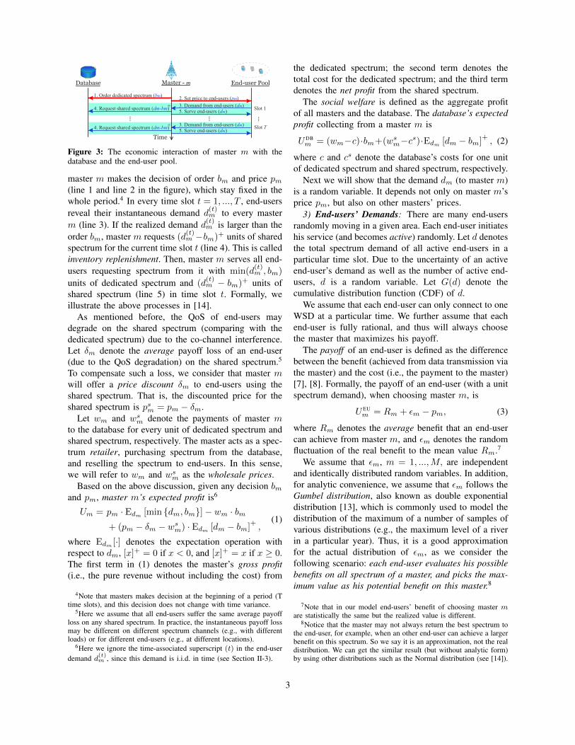
The detailed economic interaction between a master mand the database as well as end-users is illustrated inFigure 3. We consider the interactions in a period ofT time slots.3 At the beginning of the period, every

3A time slot is the minimum time unit of scheduling. The end-userdemand remains unchanged in one slot, but may change across slots.

2

Time

2. Set price to end-users (pm) 1. Order dedicated spectrum (bm)

3. Demand from end-users (dm) 4. Request shared spectrum (dm-bm) 5. Serve end-users (dm) Slot 1

Slot T

End-user PoolMaster - mDatabase

3. Demand from end-users (dm) 4. Request shared spectrum (dm-bm) 5. Serve end-users (dm)

... ... ...

+

+

Figure 3: The economic interaction of master m with thedatabase and the end-user pool.

master m makes the decision of order bm and price pm(line 1 and line 2 in the figure), which stay fixed in thewhole period.4 In every time slot t = 1, ..., T , end-usersreveal their instantaneous demand d

(t)m to every master

m (line 3). If the realized demand d(t)m is larger than theorder bm, master m requests (d

(t)m −bm)+ units of shared

spectrum for the current time slot t (line 4). This is calledinventory replenishment. Then, master m serves all end-users requesting spectrum from it with min(d

(t)m , bm)

units of dedicated spectrum and (d(t)m − bm)+ units of

shared spectrum (line 5) in time slot t. Formally, weillustrate the above processes in [14].

As mentioned before, the QoS of end-users maydegrade on the shared spectrum (comparing with thededicated spectrum) due to the co-channel interference.Let δm denote the average payoff loss of an end-user(due to the QoS degradation) on the shared spectrum.5

To compensate such a loss, we consider that master mwill offer a price discount δm to end-users using theshared spectrum. That is, the discounted price for theshared spectrum is psm = pm − δm.

Let wm and wsm denote the payments of master mto the database for every unit of dedicated spectrum andshared spectrum, respectively. The master acts as a spec-trum retailer, purchasing spectrum from the database,and reselling the spectrum to end-users. In this sense,we will refer to wm and wsm as the wholesale prices.

Based on the above discussion, given any decision bmand pm, master m’s expected profit is6

Um = pm · Edm [min {dm, bm}]− wm · bm+ (pm − δm − wsm) · Edm [dm − bm]

+,

(1)

where Edm [·] denotes the expectation operation withrespect to dm, [x]+ = 0 if x < 0, and [x]+ = x if x ≥ 0.The first term in (1) denotes the master’s gross profit(i.e., the pure revenue without including the cost) from

4Note that masters makes decision at the beginning of a period (Ttime slots), and this decision does not change with time variance.

5Here we assume that all end-users suffer the same average payoffloss on any shared spectrum. In practice, the instantaneous payoff lossmay be different on different spectrum channels (e.g., with differentloads) or for different end-users (e.g., at different locations).

6Here we ignore the time-associated superscript (t) in the end-userdemand d(t)m , since this demand is i.i.d. in time (see Section II-3).

the dedicated spectrum; the second term denotes thetotal cost for the dedicated spectrum; and the third termdenotes the net profit from the shared spectrum.

The social welfare is defined as the aggregate profitof all masters and the database. The database’s expectedprofit collecting from a master m is

U DBm = (wm−c)·bm+(wsm−cs)·Edm [dm − bm]

+, (2)

where c and cs denote the database’s costs for one unitof dedicated spectrum and shared spectrum, respectively.

Next we will show that the demand dm (to master m)is a random variable. It depends not only on master m’sprice pm, but also on other masters’ prices.

3) End-users’ Demands: There are many end-usersrandomly moving in a given area. Each end-user initiateshis service (and becomes active) randomly. Let d denotesthe total spectrum demand of all active end-users in aparticular time slot. Due to the uncertainty of an activeend-user’s demand as well as the number of active end-users, d is a random variable. Let G(d) denote thecumulative distribution function (CDF) of d.

We assume that each end-user can only connect to oneWSD at a particular time. We further assume that eachend-user is fully rational, and thus will always choosethe master that maximizes his payoff.

The payoff of an end-user is defined as the differencebetween the benefit (achieved from data transmission viathe master) and the cost (i.e., the payment to the master)[7], [8]. Formally, the payoff of an end-user (with a unitspectrum demand), when choosing master m, is

U EUm = Rm + εm − pm, (3)

where Rm denotes the average benefit that an end-usercan achieve from master m, and εm denotes the randomfluctuation of the real benefit to the mean value Rm.7

We assume that εm, m = 1, ...,M, are independentand identically distributed random variables. In addition,for analytic convenience, we assume that εm follows theGumbel distribution, also known as double exponentialdistribution [13], which is commonly used to model thedistribution of the maximum of a number of samples ofvarious distributions (e.g., the maximum level of a riverin a particular year). Thus, it is a good approximationfor the actual distribution of εm, as we consider thefollowing scenario: each end-user evaluates his possiblebenefits on all spectrum of a master, and picks the max-imum value as his potential benefit on this master.8

7Note that in our model end-users’ benefit of choosing master mare statistically the same but the realized value is different.

8Notice that the master may not always return the best spectrum tothe end-user, for example, when an other end-user can achieve a largerbenefit on this spectrum. So we say it is an approximation, not the realdistribution. We can get the similar result (but without analytic form)by using other distributions such as the Normal distribution (see [14]).

3

From the above, the average probability of an end-userchoosing a master m is given by9

θm = PR{U EUm ≥ 0 & U EU

m ≥ maxi∈M

U EUi

}= eRm−pm

1+∑

i∈M eRi−pi.

(4)

Note that 1−∑m∈M θm = 1

1+∑

i∈M eRi−pidenotes the

drop probability of an end-user (i.e., not choosing anymaster). Obviously, θm depends not only on master m’sown price pm, but also on other masters’ prices. Thus,we will also write θm as θm(p1, ..., pM ).

Note that such a probabilistic selection does not meanthat an end-user will frequently change its choice. Infact, at a particular time slot (with a period range fromseveral seconds to minutes), an end-user may stick to onemaster based on his location, service, masters’ prices,etc. The value θm is mainly used to characterize thebehavior of end-users from the system’s perspective.Thus, the total end-user demand of master m is

dm(p1, ..., pM ) = d · θm(p1, ..., pM ), (5)

which is a random variable related to all masters’ prices.

III. MONOPOLY NETWORK SCENARIO

In this section, we consider the monopoly networkscenario, where each master faces a separate pool of end-users, and thus there is no competition among masters.This case study will serve as a benchmark.

Without loss of generality, we consider a master m.Since master m acts as the monopoly provider, thedemand dm depends only on its own pm, i.e.,

dm(pm) = d · θm(pm) = d · eRm−pm

1+eRm−pm, (6)

Notice that d is a random variable with a CDF G(d).Under a price pm, the CDF of dm is

Hm(dm|pm) = G(

dmθm(pm)

). (7)

The master m’s optimal decision is given bymax

{bm≥0,pm≥0}Um(bm, pm) (8)

where Um(bm, pm) is defined in (1).We first notice that Um(bm, pm) is strictly concave

in bm. Thus, given any price pm, the optimal orderquantity b∗m can be derived by checking the necessaryand sufficient Karush-Kuhn-Tucker (KKT) condition.

Proposition 1 (Order Quantity). Given pm, master m’soptimal order quantity of dedicated spectrum is:

b∗m(pm) = H−1m(1− wm

δm+wsm|pm), (9)

if δm + wsm > wm, and b∗m(pm) = 0 otherwise.

Intuitively, we can view wsm + δm as the total cost ofone unit of shared spectrum, including both the paymentto the database and the discount to the end-users. Thus, if

9The 2nd line follows from double exponential distribution of εm.

δm +wsm ≤ wm, there is no incentive for master to pre-order any dedicated spectrum. In this rest of the paper,we will ignore this trivial case, and assume that δm +wsm > wm, i.e., the unit cost of dedicated spectrum isno larger than that of shared spectrum.

Substituting (9) into (1), we can rewrite master m’sexpected profit as a function of pm only, denoted by

Um(pm) = pm · µm − wm ·H−1m (τm|pm)

− (δm + wsm) · Edm[dm −H−1m (τm|pm)

]+,

(10)

where τm = 1 − wm

δm+wsm

, and µm = Edm [dm] =

θm(pm) · Ed[d] is the expected demand to master m.By (7), we have: H−1m (x|pm) = θm(pm) · G−1(x).

Thus, we can further rewrite (10) as

Um(pm) = (pm · µ− wm) · θm(pm), (11)

where µ = Ed[d] is the expected total demand, and wmis the virtual cost of master m, defined by

wm = wm ·G−1(τm)

+ (δm + wsm) · Ed[d−G−1(τm)

]+.

(12)

Obviously, wm is independent of pm, and is concavelyincreasing with wm, wsm, and δm.

By (11), we can easily check that ∂2Um(pm)∂p2m

≤ 0, that

is, Um(pm) is strictly concave in pm. Thus, the optimalprice p∗m can be solved by the KKT analysis.

Proposition 2 (Optimal Price). The optimal price p∗mfor a monopoly master m is given by:

µ · θm(pm) + (pm · µ− wm) · θ′m(pm) = 0. (13)

The first term in (13) denotes the marginal profitincrease due to the price increase; the second term de-notes the marginal profit decrease due to the probabilitydecrease induced by the price increase. Proposition 2states that the optimal price p∗m would equalize themarginal profit increase and decrease.

IV. COMPETITIVE NETWORK SCENARIO

In this section, we consider the general competitivenetwork scenario, where M masters compete for thesame pool of end-users. We formulate the competitionamong masters as a non-cooperative game, and study theequilibrium behavior of masters.

A. Price-Quantity Competition Game

Each master’s strategy is to determine the orderquantity of dedicated spectrum, and the price to theend-users, considering the strategies of other masters.Therefore, we formulate the interaction of masters asa non-cooperative game, called Price-Quantity compe-tition game (PQ-game). We denote the PQ-game byΓ = (M, {(bm, pm)}m∈M, {Um}m∈M), where• M is the set of game players (masters);

4

• (bm, pm) is the strategy of master m;• Um is the payoff of master m given in (1).

For notational convenience, we denote p = (p1, ..., pM )as the vector of all masters’ prices, and b = (b1, ..., bM )as the vector of all masters’ order quantities. Besides, wedenote p−m = (p1, ...pm−1, pm+1, ...pM ) and b−m =(b1, ...bm−1, bm+1, ...bM ) as the price and order vectorsof all masters except m, respectively.

In the competitive scenario, a master m’s receiveddemand dm depends not only on its own pm, but alsoon other masters’ prices p−m. By Section II-3, we have

dm(p) = d · θm(p) = d · eRm−pm

1+∑

i∈M eRi−pi, (14)

where d is the total demand of all active end-users withthe CDF G(d). Then, under any price vector p, the CDFof dm is given by

Hm(dm|p) = G(

dmθm(p)

). (15)

Substituting (14) and (15) into (1), we can easily findthat every master m’s profit Um depends not only on itsown strategy, but also on the strategies of other masters.Thus, we can write Um as Um(b,p) more precisely.

Given all other masters’ strategies p−m and b−m,master m’s best response correspondence is given by

Bm(b−m,p−m) =

arg max{bm≥0,pm≥0}

Um(bm, pm, b−m,p−m). (16)

A Nash equilibrium (NE) is such a strategy profile{b∗,p∗} that satisfies (b∗m, p

∗m) ∈ Bm(p∗−m, b

∗−m) for

all m ∈M. That is, every master’s strategy is in its bestresponse correspondence to other masters’ strategies.

B. Optimal Order Quantity

We first consider every master’s optimal order quantity(of dedicated spectrum), given the price vector p of allmasters. Similar to Proposition 1, we have

Proposition 3 (Optimal Order Quantity). Given a pricevector p, the optimal order quantity of master m is

b∗m(p) = H−1m(1− wm

δm+wsm|p)

(17)

if δm + wsm > wm, and b∗m(p) = 0 otherwise .

Similar to the monopoly scenario, we focus on thecase of δm+wsm > wm. By Proposition 3, the master m’soptimal order quantity b∗m is a function of p. Substituting(17) into (1), we can rewrite the master m’s profit asa function of p. Hence, we can transform the originalprice-quantity competition game into an equivalent pricecompetition game (where masters decide prices p only).

Formally, we denote the reduced price competitiongame as Γ = (M, {pm}m∈M, {Um}m∈M), where Umis the master m’s profit as a function of p, i.e.,

Um(p) = (pm · µ− wm) · θm(p), (18)

where τm = 1− wm

δm+wsm

, µ = Ed[d], and wm is virtualcost of master m, which has the same form as in (12).

The following proposition shows that once we find theNE of the reduced game Γ, then the NE of the originalgame Γ can be characterized immediately.

Proposition 4. If p∗ is a NE of the reduced game Γ,then {b∗(p∗),p∗} is a NE of the original game Γ, whereb∗(p∗) is the order quantity given in Proposition 3.

C. Existence and Uniqueness of Nash Equilibrium

We study the NE by using the property of supermodu-lar game [10]. There are several appealing properties fora supermodular game. First, it guarantees at least oneNE. Second, if the NE is unique, a simple best responsebased algorithm globally converges to the NE.

Theorem 1 (Existence). There exists at least one NEp∗ for the reduce price competition game Γ, and thus atleast one NE (b∗(p∗),p∗) for the original PQ-game Γ.

Here is the proof sketch of Theorem 1. First, wedefine the log-transformed game of the reduced gameΓ, denoted by Γ = (M, {pm}m∈M, {log Um}m∈M). Itis easy to prove that Γ is a supermodular game, and thushas at least one NE. Second, by the property of monotonetransformation [11], an NE of the log-transformed gameis also an NE of the original game. Hence, we canshow the existence of NE for the reduced game Γ. ByProposition 4, we can further show the existence of NEfor the original game Γ.

We can further show that the NE is unique.

Theorem 2 (Uniqueness). There is a unique NE p∗ forthe reduced game Γ, and thus a unique NE (b∗(p∗),p∗)in the original PQ-game Γ.

Similarly, We give a proof sketch of Theorem 2. Wefirst show that the log-transformed game Γ has a uniqueNE by verifying the following property [12]:

−∂2log Um(p)∂pm2 ≥

∑j 6=m

∂2log Um(p)∂pm∂pj

,∀m ∈M. (19)

By the monotone transformation [11], the reduced gameΓ has a unique NE, so does the original PQ-game Γ.

D. Algorithm

We have shown that the reduced game Γ is a log-supermodular game. and has a unique NE p∗. Hence, wecan compute p∗ by the following best response algorithm[10]: Starting with an arbitrary price vector p(0). Atevery round k + 1, each master m updates its pricebased on its best response to other masters’ prices inthe previous round k. That is,

pm(k + 1) = arg maxpm

Um(pm,p−m(k)). (20)

The above procedure continues until the NE is reached.The detailed algorithm is in our technical report [14].

5

Central 10 11 12 13 14 15 160

600

SocialW

elfare

Wholesale Price – wm

Monopoly

Monopoly

Centralized Benchmark

Competitive

Competitive

Central 10 11 12 13 14 15 160

600

MasterPro

fit

Wholesa le Price – wm

Centralized Benchmark

Competitive

Monopoly

Competitive

Monopoly

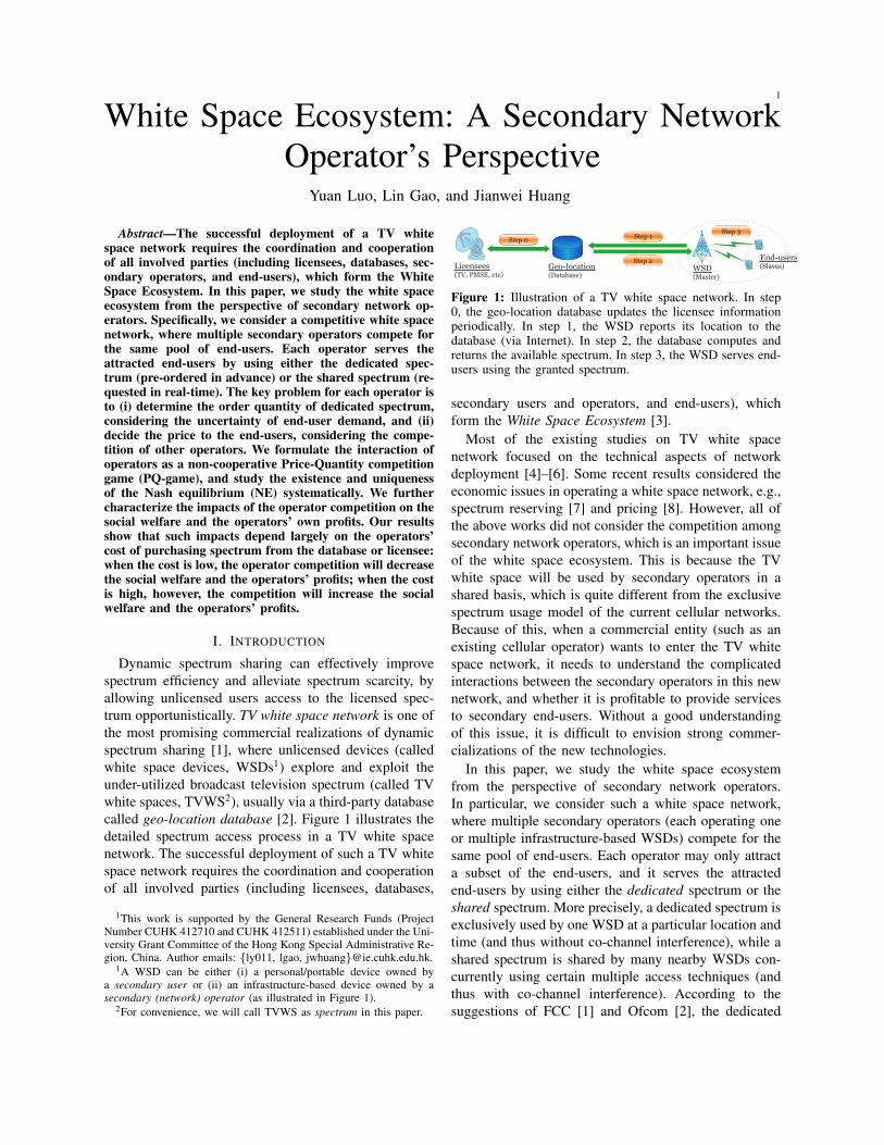
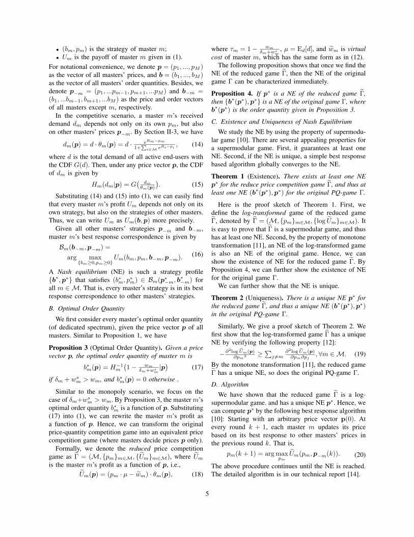
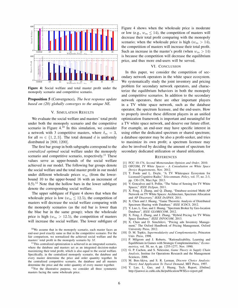
Figure 4: Social welfare and total master profit under themonopoly scenario and competitive scenario.

Proposition 5 (Convergence). The best response updatebased on (20) globally converges to the unique NE.

V. SIMULATION RESULTS

We evaluate the social welfare and masters’ total profitunder both the monopoly scenario and the competitivescenario in Figure 4.10 In this simulation, we considera network with 3 competitive masters, where δm = 3,for all m ∈ {1, 2, 3}. The total demand d is uniformlydistributed in [800, 1200].

The first bar group in both subgraphs correspond to thecentralized optimal social welfare under the monopolyscenario and competitive scenario, respectively.11 Thesevalues serve as upper-bounds of the social welfareachieved in our model. The following bar groups denotethe social welfare and the total master profit in our modelunder different wholesale prices wm (from the lower-bound 10 to the upper-bound 16 with an increment of0.5).12 Note that the hollow bars in the lower subfiguredenote the corresponding social welfare.

The upper subfigure of Figure 4 shows that when thewholesale price is low (wm ≤ 12.5), the competition ofmasters will decrease the social welfare comparing withthe monopoly scenarios (as the red bar is lower thanthe blue bar in the same group); when the wholesaleprice is high (wm > 12.5), the competition of masterswill increase the social welfare. The lower subfigure of

10We assume that in the monopoly scenario, each master faces anend-user pool exactly same as that in the competitive scenario. For thefair comparison, we normalized the achieved social welfare and themasters’ total profit in the monopoly scenario by M .

11This centralized optimization is achieved in an integrated scenario,where the database and masters act as an integrated decision-makermaximizing their total profit, which is also equal to the social welfare.Specifically, in the centralized monopoly scenario, the database andevery master determine the price and order quantity together. Inthe centralized competitive scenario, the database and all mastersdetermine the price and the order quantity of every master together.

12For the illustrative purpose, we consider all three symmetricmasters facing the same wholesale price.

Figure 4 shows when the wholesale price is moderateor low (e.g., wm ≤ 14), the competition of masters willdecrease their total profit comparing with the monopolyscenario; when the wholesale price is high (wm > 14),the competition of masters will increase their total profit.Such an increase in the master’s profit (when wm > 14)is because the competition will decrease the equilibriumprice, and thus more end-users will be served.

VI. CONCLUSION

In this paper, we consider the competition of sec-ondary network operators in the white space ecosystem.We systematically study the joint inventory and pricingproblem for secondary network operators, and charac-terize the equilibrium behaviors in both the monopolyand competitive scenarios. In addition to the secondarynetwork operators, there are other important playersin a TV white space network, such as the databaseoperator, the spectrum licensee, and the end-users. Howto properly involve these different players in an unifiedoptimization framework is important and meaningful fora TV white space network, and deserve our future effort.For example, an end-user may have specific interest inusing either the dedicated spectrum or shared spectrum;a database operator may be also a profit-seeker, and triesto maximize its own profit; a spectrum licensee mayalso be involved by deciding the amount of spectrum forsecondary dedicated utilization or shared utilization.

REFERENCES

[1] FCC 10-174, Second Memorandum Opinion and Order, 2010.[2] OFCOM, TV White Spaces - A Consultation on White Space

Device Requirements, Nov. 2012.[3] T. Forde and L. Doyle, “A TV Whitespace Ecosystem for

Licensed Cognitive Radio,” Telecommum. Policy, vol. 37, no. 2-3,pp. 130-139, Mar./Apr. 2013.

[4] V. Goncalves and S. Pollin, “The Value of Sensing for TV WhiteSpaces,” IEEE DySpan, 2011.

[5] X. Feng, J. Zhang, and Q. Zhang, “Database-assisted Multi-APNetwork on TV White Spaces: Architecture, Spectrum Allocationand AP Discovery,” IEEE DySPAN, 2011.

[6] X. Chen and J. Huang, “Game Theoretic Analysis of DistributedSpectrum Sharing with Database,” IEEE ICDCS, 2012.

[7] Y. Luo, L. Gao, and J. Huang, ”Spectrum Broker by Geo-locationDatabase”, IEEE GLOBECOM, 2012.

[8] X. Feng, J. Zhang, and J. Zhang, “Hybrid Pricing for TV WhiteSpace Database,” IEEE INFOCOM, 2013.

[9] X. Chen and D. Simchilevi, “Pricing adn Inventory Manage-ment,” The Oxford Handbook of Pricing Management, OxfordUniversity Press, 2012.

[10] D. M. Topkis, Supermodularity and Complementarity, PrincetonUniv. Press, 1998.

[11] P. Milgrom and J. Roberts, “Rationalizability, Learning andEquilibrium in Games with Strategic Complementarities,” Econo-metrica, vol. 58, no. 6, pp. 1255-1277, Nov. 1990.

[12] G. P. Cachon, and S. Netessine, Game Theory in Supply ChainAnalysis, Institue for Operations Research and the ManagementSciences, 2006.

[13] M. Ben-Akiva, and S. R. Lerman, Discrete Choice Analysis:Theory And Application To Travel Demand, MIT Press, 1997.

[14] Y. Luo, L. Gao, and J. Huang, Tech. Report, [Online]http://jianwei.ie.cuhk.edu.hk/publication/WSEco-report.pdf

6