1

Usings CNNs to Estimate Depth from StereoImagery

Tyler S. Jordan, Skanda Shridhar

Abstract—This paper explores the benefit of using Convolu-tional Neural Networks in generating a disparity space image forrendering disparity maps from stereo imagery. An eight-layerfully-connected network is constructed with 3200 neurons andtrained on 250,000 positive and negative image patch samples.The disparity space image is aggregated using context-awarecross-based method. The disparity map is generated by a “winnertakes all” strategy.

Great improvements can be visually observed in comparisonto the naive subtractive plane-sweep method especially in regionswith little to no texture.

I. INTRODUCTION

Depth-based stereoscopic image rendering and 3D recon-struction has been an important area of research in multimedia,broadcasting and in computer vision. The area has received alot of attention from the broadcast research community forits applications in 3D Television (3DTV) and Free ViewpointTelevision (FTV)[9], [7], [2], [1]. Similarly, depth-based 3Dperception is an important prerequisite for computer vision,robotics and augmented reality applications[3], [4], [6]. Withthe recent advances in omnidirectional camera rigs, computa-tional methods for postproduction, and head-mounted display(HMD) technologies, VR is on its way to become the nextcinematic medium. At the core of all of these applicationsis the ability to produce precise and accurate depth maps forthe scene under consideration. The ability to generate reliabledepth maps helps in synthesizing novel views, which is a keystep in supporting these varied applications.

Humans have an innate ability to perceive depth fromstereo imagery; however, conventional stereo correspondencealgorithms are generally incapable of producing reliable densedisparity maps. In this project, we have used convolutionalneural networks to tackle the problem of matching cost com-putation in stereo estimation. This was followed by an imageprocessing pipeline that included techniques such as crossbased cross aggregation, semiglobal matching and occlusioninterpolation for disparity refinement.

II. ALGORITHM

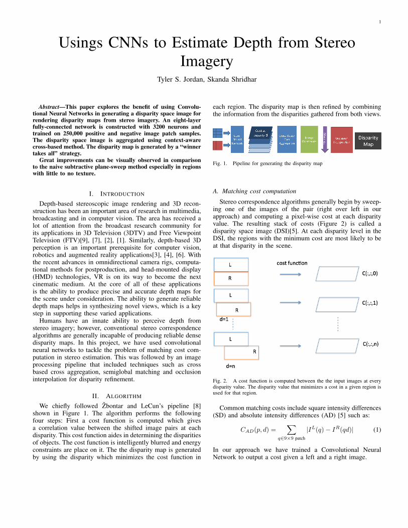
We chiefly followed Zbontar and LeCun’s pipeline [8]shown in Figure 1. The algorithm performs the followingfour steps: First a cost function is computed which givesa correlation value between the shifted image pairs at eachdisparity. This cost function aides in determining the disparitiesof objects. The cost function is intelligently blurred and energyconstraints are place on it. The the disparity map is generatedby using the disparity which minimizes the cost function in

each region. The disparity map is then refined by combiningthe information from the disparities gathered from both views.

Fig. 1. Pipeline for generating the disparity map

A. Matching cost computation

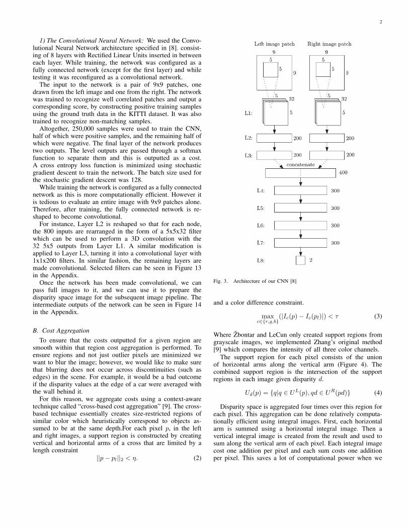
Stereo correspondence algorithms generally begin by sweep-ing one of the images of the pair (right over left in ourapproach) and computing a pixel-wise cost at each disparityvalue. The resulting stack of costs (Figure 2) is called adisparity space image (DSI)[5]. At each disparity level in theDSI, the regions with the minimum cost are most likely to beat that disparity in the scene.

Fig. 2. A cost function is computed between the the input images at everydisparity value. The disparity value that minimizes a cost in a given region isused for that region.

Common matching costs include square intensity differences(SD) and absolute intensity differences (AD) [5] such as:

CAD(p, d) =∑

q∈9×9 patch

|IL(q)− IR(qd)| (1)

In our approach we have trained a Convolutional NeuralNetwork to output a cost given a left and a right image.

2

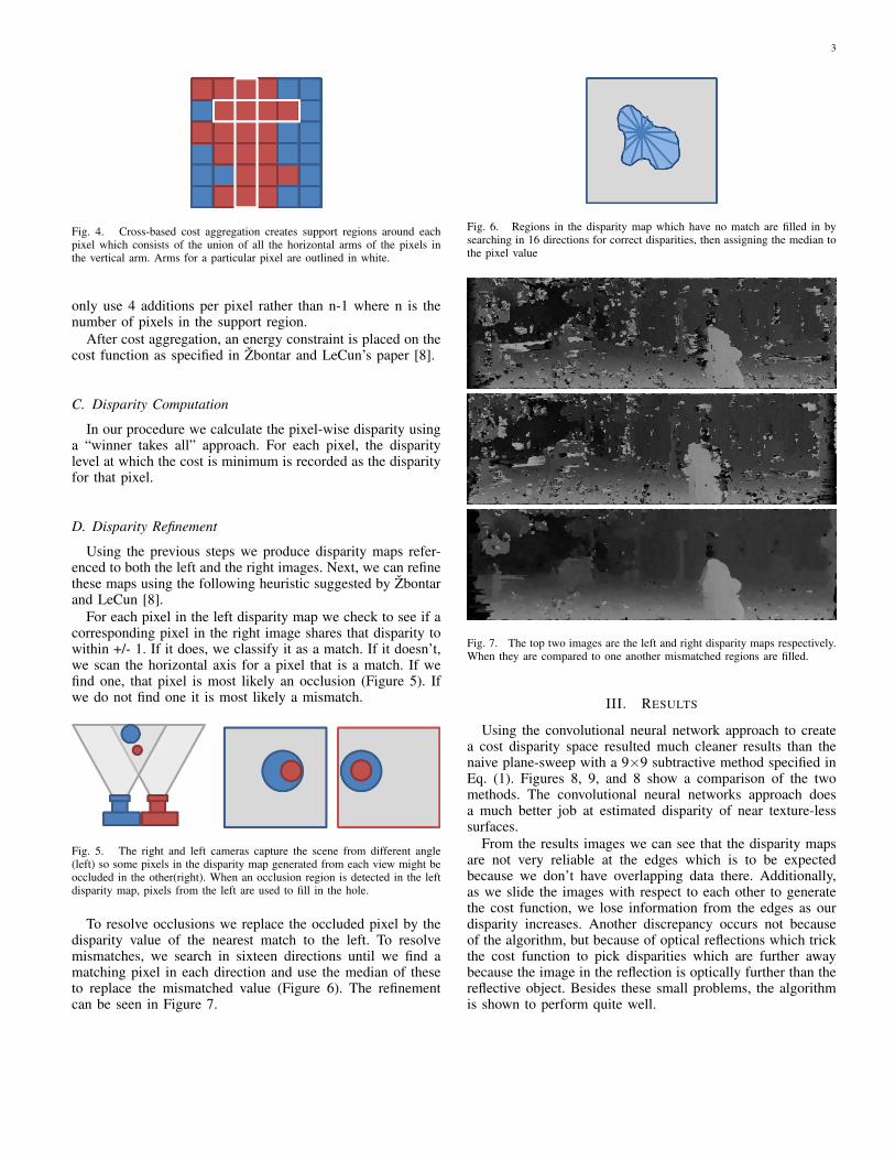
1) The Convolutional Neural Network: We used the Convo-lutional Neural Network architecture specified in [8]. consist-ing of 8 layers with Rectified Linear Units inserted in betweeneach layer. While training, the network was configured as afully connected network (except for the first layer) and whiletesting it was reconfigured as a convolutional network.

The input to the network is a pair of 9x9 patches, onedrawn from the left image and one from the right. The networkwas trained to recognize well correlated patches and output acorresponding score, by constructing positive training samplesusing the ground truth data in the KITTI dataset. It was alsotrained to recognize non-matching samples.

Altogether, 250,000 samples were used to train the CNN,half of which were positive samples, and the remaining half ofwhich were negative. The final layer of the network producestwo outputs. The level outputs are passed through a softmaxfunction to separate them and this is outputted as a cost.A cross entropy loss function is minimized using stochasticgradient descent to train the network. The batch size used forthe stochastic gradient descent was 128.

While training the network is configured as a fully connectednetwork as this is more computationally efficient. However itis tedious to evaluate an entire image with 9x9 patches alone.Therefore, after training, the fully connected network is re-shaped to become convolutional.

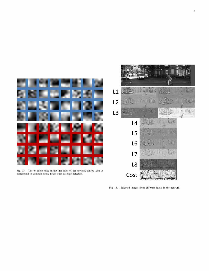
For instance, Layer L2 is reshaped so that for each node,the 800 inputs are rearranged in the form of a 5x5x32 filterwhich can be used to perform a 3D convolution with the32 5x5 outputs from Layer L1. A similar modification isapplied to Layer L3, turning it into a convolutional layer with1x1x200 filters. In similar fashion, the remaining layers aremade convolutional. Selected filters can be seen in Figure 13in the Appendix.

Once the network has been made convolutional, we canpass full images to it, and we can use it to prepare thedisparity space image for the subsequent image pipeline. Theintermediate outputs of the network can be seen in Figure 14in the Appendix.

B. Cost AggregationTo ensure that the costs outputted for a given region are

smooth within that region cost aggregation is performed. Toensure regions and not just outlier pixels are minimized wewant to blur the image; however, we would like to make surethat blurring does not occur across discontinuities (such asedges) in the scene. For example, it would be a bad outcomeif the disparity values at the edge of a car were averaged withthe wall behind it.

For this reason, we aggregate costs using a context-awaretechnique called “cross-based cost aggregation” [9]. The cross-based technique essentially creates size-restricted regions ofsimilar color which heuristically correspond to objects as-sumed to be at the same depth.For each pixel p, in the leftand right images, a support region is constructed by creatingvertical and horizontal arms of a cross that are limited by alength constraint

||p− pl||2 < η. (2)

Fig. 3. Architecture of our CNN [8]

and a color difference constraint.

maxc∈{r,g,b}

(|Ic(p)− Ic(pl)|) < τ (3)

Where Zbontar and LeCun only created support regions fromgrayscale images, we implemented Zhang’s original method[9] which compares the intensity of all three color channels.

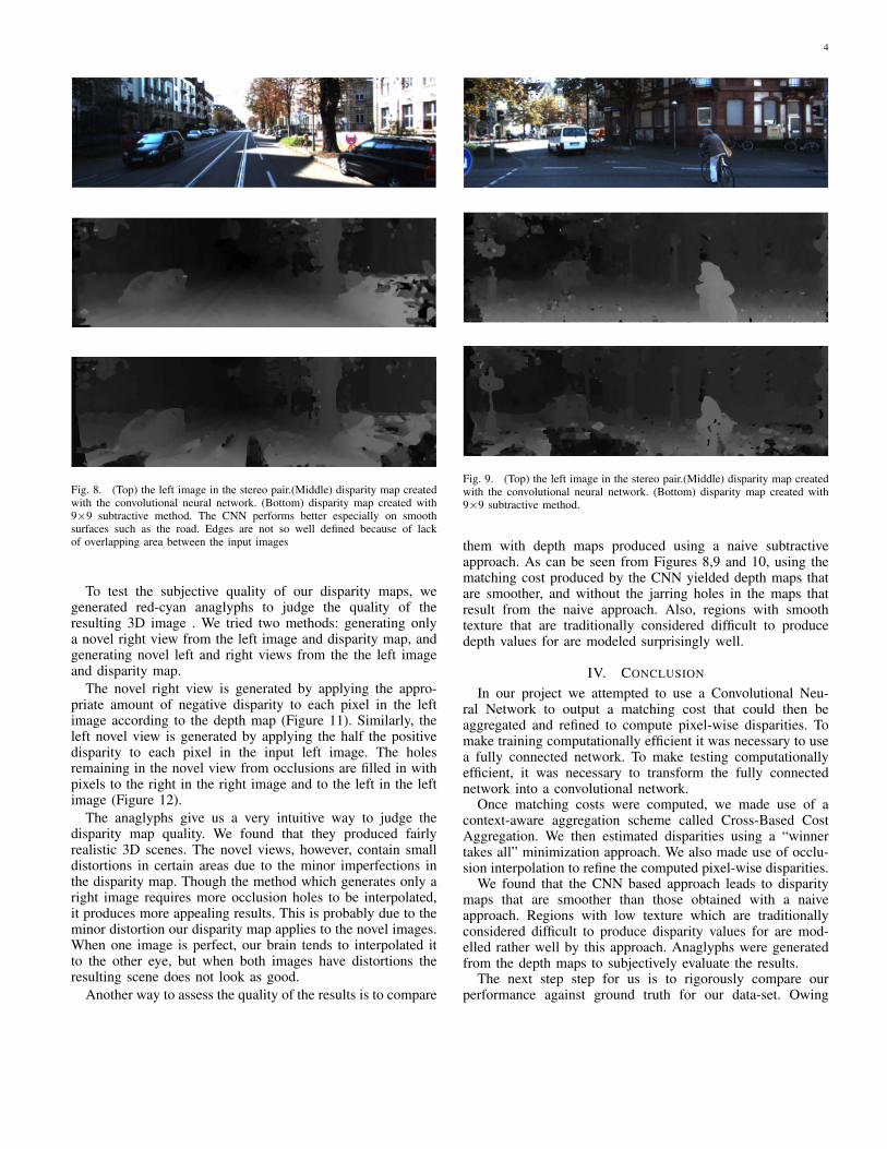
The support region for each pixel consists of the unionof horizontal arms along the vertical arm (Figure 4). Thecombined support region is the intersection of the supportregions in each image given disparity d.

Ud(p) = {q|q ∈ UL(p), qd ∈ UR(pd)} (4)

Disparity space is aggregated four times over this region foreach pixel. This aggregation can be done relatively computa-tionally efficient using integral images. First, each horizontalarm is summed using a horizontal integral image. Then avertical integral image is created from the result and used tosum along the vertical arm of each pixel. Each integral imagecost one addition per pixel and each sum costs one additionper pixel. This saves a lot of computational power when we

3

Fig. 4. Cross-based cost aggregation creates support regions around eachpixel which consists of the union of all the horizontal arms of the pixels inthe vertical arm. Arms for a particular pixel are outlined in white.

only use 4 additions per pixel rather than n-1 where n is thenumber of pixels in the support region.

After cost aggregation, an energy constraint is placed on thecost function as specified in Zbontar and LeCun’s paper [8].

C. Disparity Computation

In our procedure we calculate the pixel-wise disparity usinga “winner takes all” approach. For each pixel, the disparitylevel at which the cost is minimum is recorded as the disparityfor that pixel.

D. Disparity Refinement

Using the previous steps we produce disparity maps refer-enced to both the left and the right images. Next, we can refinethese maps using the following heuristic suggested by Zbontarand LeCun [8].

For each pixel in the left disparity map we check to see if acorresponding pixel in the right image shares that disparity towithin +/- 1. If it does, we classify it as a match. If it doesn’t,we scan the horizontal axis for a pixel that is a match. If wefind one, that pixel is most likely an occlusion (Figure 5). Ifwe do not find one it is most likely a mismatch.

Fig. 5. The right and left cameras capture the scene from different angle(left) so some pixels in the disparity map generated from each view might beoccluded in the other(right). When an occlusion region is detected in the leftdisparity map, pixels from the left are used to fill in the hole.

To resolve occlusions we replace the occluded pixel by thedisparity value of the nearest match to the left. To resolvemismatches, we search in sixteen directions until we find amatching pixel in each direction and use the median of theseto replace the mismatched value (Figure 6). The refinementcan be seen in Figure 7.

Fig. 6. Regions in the disparity map which have no match are filled in bysearching in 16 directions for correct disparities, then assigning the median tothe pixel value

Fig. 7. The top two images are the left and right disparity maps respectively.When they are compared to one another mismatched regions are filled.

III. RESULTS

Using the convolutional neural network approach to createa cost disparity space resulted much cleaner results than thenaive plane-sweep with a 9×9 subtractive method specified inEq. (1). Figures 8, 9, and 8 show a comparison of the twomethods. The convolutional neural networks approach doesa much better job at estimated disparity of near texture-lesssurfaces.

From the results images we can see that the disparity mapsare not very reliable at the edges which is to be expectedbecause we don’t have overlapping data there. Additionally,as we slide the images with respect to each other to generatethe cost function, we lose information from the edges as ourdisparity increases. Another discrepancy occurs not becauseof the algorithm, but because of optical reflections which trickthe cost function to pick disparities which are further awaybecause the image in the reflection is optically further than thereflective object. Besides these small problems, the algorithmis shown to perform quite well.

4

Fig. 8. (Top) the left image in the stereo pair.(Middle) disparity map createdwith the convolutional neural network. (Bottom) disparity map created with9×9 subtractive method. The CNN performs better especially on smoothsurfaces such as the road. Edges are not so well defined because of lackof overlapping area between the input images

To test the subjective quality of our disparity maps, wegenerated red-cyan anaglyphs to judge the quality of theresulting 3D image . We tried two methods: generating onlya novel right view from the left image and disparity map, andgenerating novel left and right views from the the left imageand disparity map.

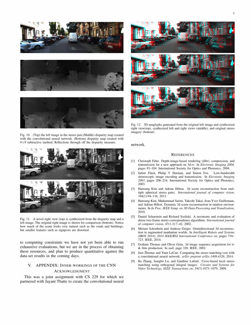
The novel right view is generated by applying the appro-priate amount of negative disparity to each pixel in the leftimage according to the depth map (Figure 11). Similarly, theleft novel view is generated by applying the half the positivedisparity to each pixel in the input left image. The holesremaining in the novel view from occlusions are filled in withpixels to the right in the right image and to the left in the leftimage (Figure 12).

The anaglyphs give us a very intuitive way to judge thedisparity map quality. We found that they produced fairlyrealistic 3D scenes. The novel views, however, contain smalldistortions in certain areas due to the minor imperfections inthe disparity map. Though the method which generates only aright image requires more occlusion holes to be interpolated,it produces more appealing results. This is probably due to theminor distortion our disparity map applies to the novel images.When one image is perfect, our brain tends to interpolated itto the other eye, but when both images have distortions theresulting scene does not look as good.

Another way to assess the quality of the results is to compare

Fig. 9. (Top) the left image in the stereo pair.(Middle) disparity map createdwith the convolutional neural network. (Bottom) disparity map created with9×9 subtractive method.

them with depth maps produced using a naive subtractiveapproach. As can be seen from Figures 8,9 and 10, using thematching cost produced by the CNN yielded depth maps thatare smoother, and without the jarring holes in the maps thatresult from the naive approach. Also, regions with smoothtexture that are traditionally considered difficult to producedepth values for are modeled surprisingly well.

IV. CONCLUSION

In our project we attempted to use a Convolutional Neu-ral Network to output a matching cost that could then beaggregated and refined to compute pixel-wise disparities. Tomake training computationally efficient it was necessary to usea fully connected network. To make testing computationallyefficient, it was necessary to transform the fully connectednetwork into a convolutional network.

Once matching costs were computed, we made use of acontext-aware aggregation scheme called Cross-Based CostAggregation. We then estimated disparities using a “winnertakes all” minimization approach. We also made use of occlu-sion interpolation to refine the computed pixel-wise disparities.

We found that the CNN based approach leads to disparitymaps that are smoother than those obtained with a naiveapproach. Regions with low texture which are traditionallyconsidered difficult to produce disparity values for are mod-elled rather well by this approach. Anaglyphs were generatedfrom the depth maps to subjectively evaluate the results.

The next step step for us is to rigorously compare ourperformance against ground truth for our data-set. Owing

5

Fig. 10. (Top) the left image in the stereo pair.(Middle) disparity map createdwith the convolutional neural network. (Bottom) disparity map created with9×9 subtractive method. Reflections through off the disparity measure.

Fig. 11. A novel right view (top) is synthesized from the disparity map and aleft image. The original right image is shown for comparison (bottom). Noticehow much of the scene looks very natural such as the roads and buildings,but smaller features such as signposts are distorted.

to computing constraints we have not yet been able to runexhaustive evaluations, but we are in the process of obtainingthese resources, and plan to produce quantitative against thedata-set results in the coming days.

V. APPENDIX: INNER-WORKINGS OF THE CNNACKNOWLEDGMENT

This was a joint assignment with CS 229 for which wepartnered with Jayant Thatte to create the convolutional neural

Fig. 12. 3D anaglyphs generated from the original left image and synthesizedright view(top), synthesized left and right views (middle), and original stereoimagery (bottom)

network.

REFERENCES

[1] Christoph Fehn. Depth-image-based rendering (dibr), compression, andtransmission for a new approach on 3d-tv. In Electronic Imaging 2004,pages 93–104. International Society for Optics and Photonics, 2004.

[2] Julien Flack, Philip V Harman, and Simon Fox. Low-bandwidthstereoscopic image encoding and transmission. In Electronic Imaging2003, pages 206–214. International Society for Optics and Photonics,2003.

[3] Hansung Kim and Adrian Hilton. 3d scene reconstruction from mul-tiple spherical stereo pairs. International journal of computer vision,104(1):94–116, 2013.

[4] Hansung Kim, Muhammad Sarim, Takeshi Takai, Jean-Yves Guillemaut,and Adrian Hilton. Dynamic 3d scene reconstruction in outdoor environ-ments. In In Proc. IEEE Symp. on 3D Data Processing and Visualization,2010.

[5] Daniel Scharstein and Richard Szeliski. A taxonomy and evaluation ofdense two-frame stereo correspondence algorithms. International journalof computer vision, 47(1-3):7–42, 2002.

[6] Miriam Schonbein and Andreas Geiger. Omnidirectional 3d reconstruc-tion in augmented manhattan worlds. In Intelligent Robots and Systems(IROS 2014), 2014 IEEE/RSJ International Conference on, pages 716–723. IEEE, 2014.

[7] Graham Thomas and Oliver Grau. 3d image sequence acquisition for tv& film production. In null, page 320. IEEE, 2002.

[8] Jure Zbontar and Yann LeCun. Computing the stereo matching cost witha convolutional neural network. arXiv preprint arXiv:1409.4326, 2014.

[9] Ke Zhang, Jiangbo Lu, and Gauthier Lafruit. Cross-based local stereomatching using orthogonal integral images. Circuits and Systems forVideo Technology, IEEE Transactions on, 19(7):1073–1079, 2009.

6

Fig. 13. The 64 filters used in the first layer of the network can be seen tocorrespond to common-sense filters such as edge-detectors.

Fig. 14. Selected images from different levels in the network