Deep Forensics: Using CNNs to Differentiate CGI fromPhotographic Images

CS89/189 Final Project

Shruti Agarwal∗

Dartmouth CollegeLiane Makatura

†

Dartmouth College

ABSTRACTAdvances in modeling, rendering and image manipulationtechnologies have made it substantially more difficult to dis-tinguish real photographs from computer generated images(CGI). The hand-crafted features we’ve been exploiting thusfar are in constant need of updating, and each new observa-tion is a rather time-intensive process. To address this, weexplored the possibility of learning some representation thatwould be capable of discriminating between these two classesdirectly from the image pixels themselves. Due to their re-cent successes in other image processing and visual recog-nition domains, we propose the use of deep convolutionalneural networks (CNNs) for this task. We also introduce anew dataset, consisting of approximately 100,000 content-matched image patches in each class (CGI, photograph) fora total dataset of roughly 200,000 patches.

KeywordsDeep Learning, Photorealistic, CGI, Image Forensics

1. INTRODUCTIONAdvances in modeling, rendering and image manipulationtechnologies have made it substantially more difficult to dis-tinguish real photographs from computer generated images(CGI). This progress is viewed positively from the perspec-tive of the artist, who has far more flexibility in terms ofthe styles that he or she is able to mimic or produce. How-ever, these advances are problematic from legal and ethicalstandpoints, where it is imperative that we be able to re-liably differentiate between original photographs and thosethat are synthetic or digitally manipulated.

Over the last few years, technological approaches have beenable to achieve impressively high levels of accuracy on thistask using hand constructed features with relatively simple

∗Shruti.Agarwal.GR@Dartmouth.edu†Liane.E.Makatura.17@Dartmouth.edu

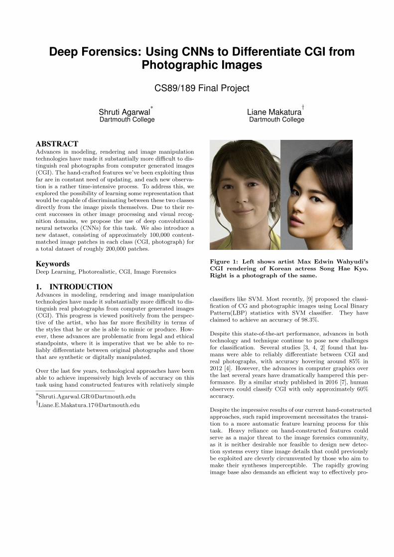
Figure 1: Left shows artist Max Edwin Wahyudi’sCGI rendering of Korean actress Song Hae Kyo.Right is a photograph of the same.

classifiers like SVM. Most recently, [9] proposed the classi-fication of CG and photographic images using Local BinaryPattern(LBP) statistics with SVM classifier. They haveclaimed to achieve an accuracy of 98.3%.

Despite this state-of-the-art performance, advances in bothtechnology and technique continue to pose new challengesfor classification. Several studies [3, 4, 2] found that hu-mans were able to reliably differentiate between CGI andreal photographs, with accuracy hovering around 85% in2012 [4]. However, the advances in computer graphics overthe last several years have dramatically hampered this per-formance. By a similar study published in 2016 [7], humanobservers could classify CGI with only approximately 60%accuracy.

Despite the impressive results of our current hand-constructedapproaches, such rapid improvement necessitates the transi-tion to a more automatic feature learning process for thistask. Heavy reliance on hand-constructed features couldserve as a major threat to the image forensics community,as it is neither desirable nor feasible to design new detec-tion systems every time image details that could previouslybe exploited are cleverly circumvented by those who aim tomake their syntheses imperceptible. The rapidly growingimage base also demands an efficient way to effectively pro-

cess and classify large quantities of vastly differing images,which may not be possible with these necessarily constrainedapproaches.

In response to these demands, we turned our attention tothe field of deep learning, which has shown considerablepromise over the past few years in similar visual recogni-tion domains – notably, image classification and semanticsegmentation. We note that the learned features of suchnetworks have demonstrated their ability to substantiallyoutperform hand-constructed features, while also exhibitingsome notion of automatic learning, which would allow thenets to be effectively retrained each time new features arerequired or desired. Noting this strong evidence, we hypoth-esize that deep convolutional neural networks (CNN) couldbe used as a tool to perform, and hopefully improve upon,this task of classifying real world photographs and CGI.

Since there is currently no suitably large, labeled CGI datasetavailable, we are limited in our ability to directly train aneural net for this task. However, recent work has shownfine-tuning to be a promising alternative for deep learningin data-scarce domains, so we hope to develop suitable fea-tures by adapting AlexNet[8] to this CGI classification do-main. We seek to measure our binary (Photograph vs. CGI(non-photograph)) classification accuracy obtained by 1) di-rectly feeding images through our finetuned network, and 2)training an SVM on the 4096-dimensional features extractedfrom the penultimate layer (fc-6) of our network.

2. RELATED WORKThe results in [1, 6, 11] demonstrated that deep featuresmay be able to effectively generalize to a variety of tasksand datasets. In [1], authors performed thorough experi-mentation to show that the visual representations learnedusing a large labelled dataset like ImageNet can be used fortasks like object recognition on the Caltech-101 dataset[5],domain adaptation on the Office dataset[10], subcategoryrecognition on the Caltech-UCSD bird dataset and scenerecognition on the SUN-397 dataset. In each case, the deepfeatures performed better than other state-of-art techniques.In one such case, we saw that 33% classification accuracyis obtained even when there was only a single labeled ex-ample per category. The R-CNN method [6] was also ableto achieve significant performance boosts after fine-tuninga network trained (in a supervised fashion) on ILSVRC forvarious data-scarce tasks like object detection on PASCALVOC.

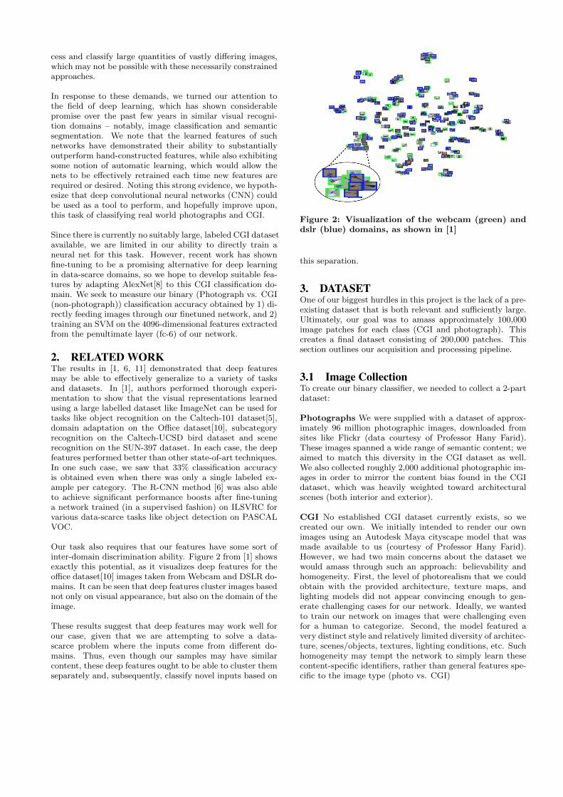
Our task also requires that our features have some sort ofinter-domain discrimination ability. Figure 2 from [1] showsexactly this potential, as it visualizes deep features for theoffice dataset[10] images taken from Webcam and DSLR do-mains. It can be seen that deep features cluster images basednot only on visual appearance, but also on the domain of theimage.

These results suggest that deep features may work well forour case, given that we are attempting to solve a data-scarce problem where the inputs come from different do-mains. Thus, even though our samples may have similarcontent, these deep features ought to be able to cluster themseparately and, subsequently, classify novel inputs based on

Figure 2: Visualization of the webcam (green) anddslr (blue) domains, as shown in [1]

this separation.

3. DATASETOne of our biggest hurdles in this project is the lack of a pre-existing dataset that is both relevant and sufficiently large.Ultimately, our goal was to amass approximately 100,000image patches for each class (CGI and photograph). Thiscreates a final dataset consisting of 200,000 patches. Thissection outlines our acquisition and processing pipeline.

3.1 Image CollectionTo create our binary classifier, we needed to collect a 2-partdataset:

Photographs We were supplied with a dataset of approx-imately 96 million photographic images, downloaded fromsites like Flickr (data courtesy of Professor Hany Farid).These images spanned a wide range of semantic content; weaimed to match this diversity in the CGI dataset as well.We also collected roughly 2,000 additional photographic im-ages in order to mirror the content bias found in the CGIdataset, which was heavily weighted toward architecturalscenes (both interior and exterior).

CGI No established CGI dataset currently exists, so wecreated our own. We initially intended to render our ownimages using an Autodesk Maya cityscape model that wasmade available to us (courtesy of Professor Hany Farid).However, we had two main concerns about the dataset wewould amass through such an approach: believability andhomogeneity. First, the level of photorealism that we couldobtain with the provided architecture, texture maps, andlighting models did not appear convincing enough to gen-erate challenging cases for our network. Ideally, we wantedto train our network on images that were challenging evenfor a human to categorize. Second, the model featured avery distinct style and relatively limited diversity of architec-ture, scenes/objects, textures, lighting conditions, etc. Suchhomogeneity may tempt the network to simply learn thesecontent-specific identifiers, rather than general features spe-cific to the image type (photo vs. CGI)

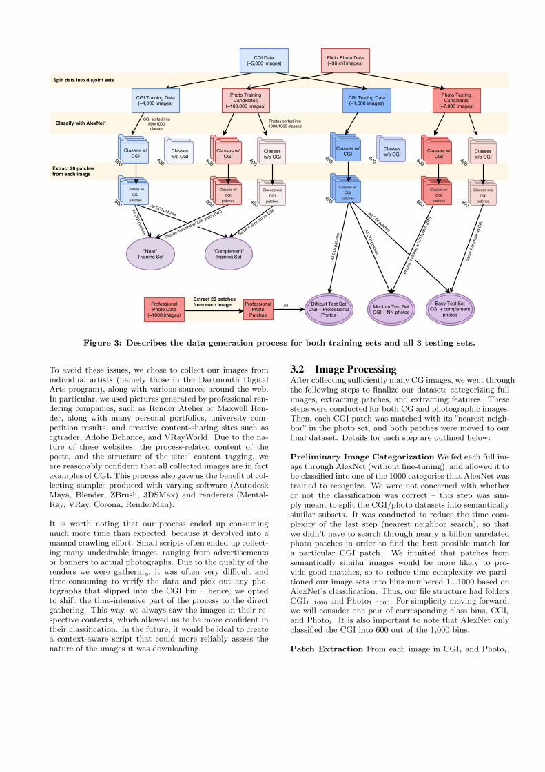
Figure 3: Describes the data generation process for both training sets and all 3 testing sets.

To avoid these issues, we chose to collect our images fromindividual artists (namely those in the Dartmouth DigitalArts program), along with various sources around the web.In particular, we used pictures generated by professional ren-dering companies, such as Render Atelier or Maxwell Ren-der, along with many personal portfolios, university com-petition results, and creative content-sharing sites such ascgtrader, Adobe Behance, and VRayWorld. Due to the na-ture of these websites, the process-related content of theposts, and the structure of the sites’ content tagging, weare reasonably confident that all collected images are in factexamples of CGI. This process also gave us the benefit of col-lecting samples produced with varying software (AutodeskMaya, Blender, ZBrush, 3DSMax) and renderers (Mental-Ray, VRay, Corona, RenderMan).

It is worth noting that our process ended up consumingmuch more time than expected, because it devolved into amanual crawling effort. Small scripts often ended up collect-ing many undesirable images, ranging from advertisementsor banners to actual photographs. Due to the quality of therenders we were gathering, it was often very difficult andtime-consuming to verify the data and pick out any pho-tographs that slipped into the CGI bin – hence, we optedto shift the time-intensive part of the process to the directgathering. This way, we always saw the images in their re-spective contexts, which allowed us to be more confident intheir classification. In the future, it would be ideal to createa context-aware script that could more reliably assess thenature of the images it was downloading.

3.2 Image ProcessingAfter collecting sufficiently many CG images, we went throughthe following steps to finalize our dataset: categorizing fullimages, extracting patches, and extracting features. Thesesteps were conducted for both CG and photographic images.Then, each CGI patch was matched with its ”nearest neigh-bor” in the photo set, and both patches were moved to ourfinal dataset. Details for each step are outlined below:

Preliminary Image Categorization We fed each full im-age through AlexNet (without fine-tuning), and allowed it tobe classified into one of the 1000 categories that AlexNet wastrained to recognize. We were not concerned with whetheror not the classification was correct – this step was sim-ply meant to split the CGI/photo datasets into semanticallysimilar subsets. It was conducted to reduce the time com-plexity of the last step (nearest neighbor search), so thatwe didn’t have to search through nearly a billion unrelatedphoto patches in order to find the best possible match fora particular CGI patch. We intuited that patches fromsemantically similar images would be more likely to pro-vide good matches, so to reduce time complexity we parti-tioned our image sets into bins numbered 1...1000 based onAlexNet’s classification. Thus, our file structure had foldersCGI1..1000 and Photo1..1000. For simplicity moving forward,we will consider one pair of corresponding class bins, CGIiand Photoi. It is also important to note that AlexNet onlyclassified the CGI into 600 out of the 1,000 bins.

Patch Extraction From each image in CGIi and Photoi,

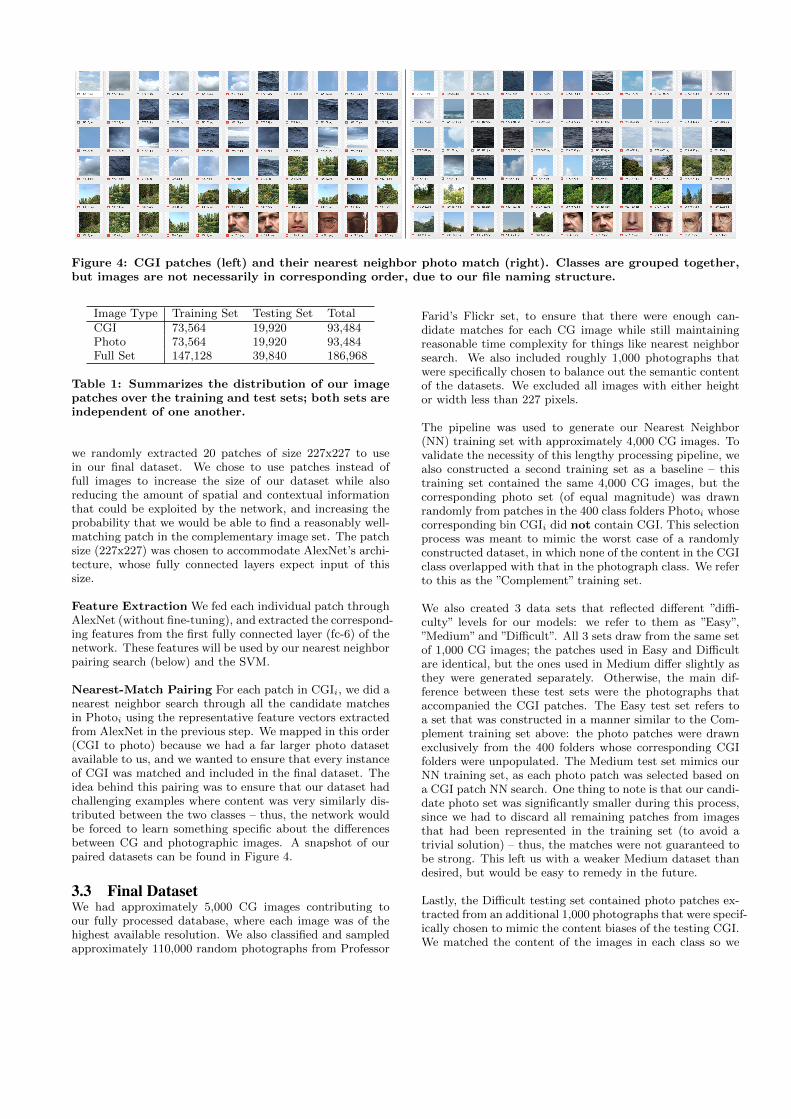
Figure 4: CGI patches (left) and their nearest neighbor photo match (right). Classes are grouped together,but images are not necessarily in corresponding order, due to our file naming structure.

Image Type Training Set Testing Set TotalCGI 73,564 19,920 93,484Photo 73,564 19,920 93,484Full Set 147,128 39,840 186,968

Table 1: Summarizes the distribution of our imagepatches over the training and test sets; both sets areindependent of one another.

we randomly extracted 20 patches of size 227x227 to usein our final dataset. We chose to use patches instead offull images to increase the size of our dataset while alsoreducing the amount of spatial and contextual informationthat could be exploited by the network, and increasing theprobability that we would be able to find a reasonably well-matching patch in the complementary image set. The patchsize (227x227) was chosen to accommodate AlexNet’s archi-tecture, whose fully connected layers expect input of thissize.

Feature Extraction We fed each individual patch throughAlexNet (without fine-tuning), and extracted the correspond-ing features from the first fully connected layer (fc-6) of thenetwork. These features will be used by our nearest neighborpairing search (below) and the SVM.

Nearest-Match Pairing For each patch in CGIi, we did anearest neighbor search through all the candidate matchesin Photoi using the representative feature vectors extractedfrom AlexNet in the previous step. We mapped in this order(CGI to photo) because we had a far larger photo datasetavailable to us, and we wanted to ensure that every instanceof CGI was matched and included in the final dataset. Theidea behind this pairing was to ensure that our dataset hadchallenging examples where content was very similarly dis-tributed between the two classes – thus, the network wouldbe forced to learn something specific about the differencesbetween CG and photographic images. A snapshot of ourpaired datasets can be found in Figure 4.

3.3 Final DatasetWe had approximately 5,000 CG images contributing toour fully processed database, where each image was of thehighest available resolution. We also classified and sampledapproximately 110,000 random photographs from Professor

Farid’s Flickr set, to ensure that there were enough can-didate matches for each CG image while still maintainingreasonable time complexity for things like nearest neighborsearch. We also included roughly 1,000 photographs thatwere specifically chosen to balance out the semantic contentof the datasets. We excluded all images with either heightor width less than 227 pixels.

The pipeline was used to generate our Nearest Neighbor(NN) training set with approximately 4,000 CG images. Tovalidate the necessity of this lengthy processing pipeline, wealso constructed a second training set as a baseline – thistraining set contained the same 4,000 CG images, but thecorresponding photo set (of equal magnitude) was drawnrandomly from patches in the 400 class folders Photoi whosecorresponding bin CGIi did not contain CGI. This selectionprocess was meant to mimic the worst case of a randomlyconstructed dataset, in which none of the content in the CGIclass overlapped with that in the photograph class. We referto this as the ”Complement” training set.

We also created 3 data sets that reflected different ”diffi-culty” levels for our models: we refer to them as ”Easy”,”Medium” and ”Difficult”. All 3 sets draw from the same setof 1,000 CG images; the patches used in Easy and Difficultare identical, but the ones used in Medium differ slightly asthey were generated separately. Otherwise, the main dif-ference between these test sets were the photographs thataccompanied the CGI patches. The Easy test set refers toa set that was constructed in a manner similar to the Com-plement training set above: the photo patches were drawnexclusively from the 400 folders whose corresponding CGIfolders were unpopulated. The Medium test set mimics ourNN training set, as each photo patch was selected based ona CGI patch NN search. One thing to note is that our candi-date photo set was significantly smaller during this process,since we had to discard all remaining patches from imagesthat had been represented in the training set (to avoid atrivial solution) – thus, the matches were not guaranteed tobe strong. This left us with a weaker Medium dataset thandesired, but would be easy to remedy in the future.

Lastly, the Difficult testing set contained photo patches ex-tracted from an additional 1,000 photographs that were specif-ically chosen to mimic the content biases of the testing CGI.We matched the content of the images in each class so we

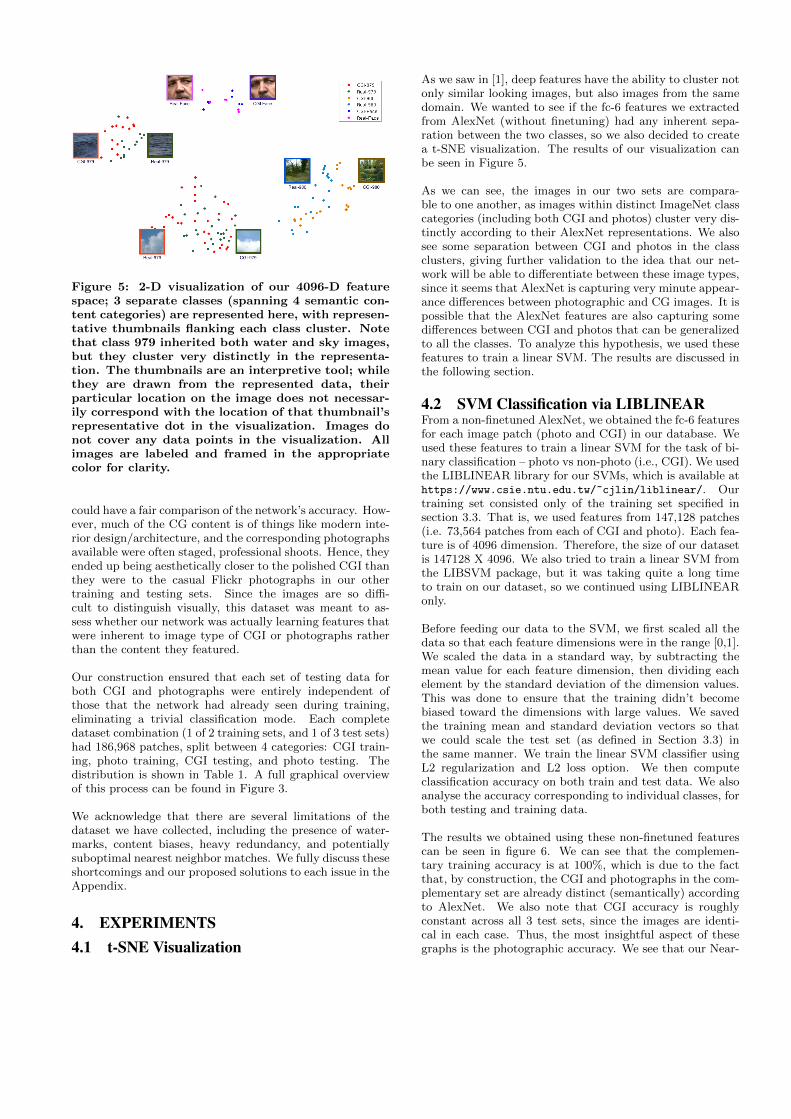
Figure 5: 2-D visualization of our 4096-D featurespace; 3 separate classes (spanning 4 semantic con-tent categories) are represented here, with represen-tative thumbnails flanking each class cluster. Notethat class 979 inherited both water and sky images,but they cluster very distinctly in the representa-tion. The thumbnails are an interpretive tool; whilethey are drawn from the represented data, theirparticular location on the image does not necessar-ily correspond with the location of that thumbnail’srepresentative dot in the visualization. Images donot cover any data points in the visualization. Allimages are labeled and framed in the appropriatecolor for clarity.

could have a fair comparison of the network’s accuracy. How-ever, much of the CG content is of things like modern inte-rior design/architecture, and the corresponding photographsavailable were often staged, professional shoots. Hence, theyended up being aesthetically closer to the polished CGI thanthey were to the casual Flickr photographs in our othertraining and testing sets. Since the images are so diffi-cult to distinguish visually, this dataset was meant to as-sess whether our network was actually learning features thatwere inherent to image type of CGI or photographs ratherthan the content they featured.

Our construction ensured that each set of testing data forboth CGI and photographs were entirely independent ofthose that the network had already seen during training,eliminating a trivial classification mode. Each completedataset combination (1 of 2 training sets, and 1 of 3 test sets)had 186,968 patches, split between 4 categories: CGI train-ing, photo training, CGI testing, and photo testing. Thedistribution is shown in Table 1. A full graphical overviewof this process can be found in Figure 3.

We acknowledge that there are several limitations of thedataset we have collected, including the presence of water-marks, content biases, heavy redundancy, and potentiallysuboptimal nearest neighbor matches. We fully discuss theseshortcomings and our proposed solutions to each issue in theAppendix.

4. EXPERIMENTS4.1 t-SNE Visualization

As we saw in [1], deep features have the ability to cluster notonly similar looking images, but also images from the samedomain. We wanted to see if the fc-6 features we extractedfrom AlexNet (without finetuning) had any inherent sepa-ration between the two classes, so we also decided to createa t-SNE visualization. The results of our visualization canbe seen in Figure 5.

As we can see, the images in our two sets are compara-ble to one another, as images within distinct ImageNet classcategories (including both CGI and photos) cluster very dis-tinctly according to their AlexNet representations. We alsosee some separation between CGI and photos in the classclusters, giving further validation to the idea that our net-work will be able to differentiate between these image types,since it seems that AlexNet is capturing very minute appear-ance differences between photographic and CG images. It ispossible that the AlexNet features are also capturing somedifferences between CGI and photos that can be generalizedto all the classes. To analyze this hypothesis, we used thesefeatures to train a linear SVM. The results are discussed inthe following section.

4.2 SVM Classification via LIBLINEARFrom a non-finetuned AlexNet, we obtained the fc-6 featuresfor each image patch (photo and CGI) in our database. Weused these features to train a linear SVM for the task of bi-nary classification – photo vs non-photo (i.e., CGI). We usedthe LIBLINEAR library for our SVMs, which is available athttps://www.csie.ntu.edu.tw/~cjlin/liblinear/. Ourtraining set consisted only of the training set specified insection 3.3. That is, we used features from 147,128 patches(i.e. 73,564 patches from each of CGI and photo). Each fea-ture is of 4096 dimension. Therefore, the size of our datasetis 147128 X 4096. We also tried to train a linear SVM fromthe LIBSVM package, but it was taking quite a long timeto train on our dataset, so we continued using LIBLINEARonly.

Before feeding our data to the SVM, we first scaled all thedata so that each feature dimensions were in the range [0,1].We scaled the data in a standard way, by subtracting themean value for each feature dimension, then dividing eachelement by the standard deviation of the dimension values.This was done to ensure that the training didn’t becomebiased toward the dimensions with large values. We savedthe training mean and standard deviation vectors so thatwe could scale the test set (as defined in Section 3.3) inthe same manner. We train the linear SVM classifier usingL2 regularization and L2 loss option. We then computeclassification accuracy on both train and test data. We alsoanalyse the accuracy corresponding to individual classes, forboth testing and training data.

The results we obtained using these non-finetuned featurescan be seen in figure 6. We can see that the complemen-tary training accuracy is at 100%, which is due to the factthat, by construction, the CGI and photographs in the com-plementary set are already distinct (semantically) accordingto AlexNet. We also note that CGI accuracy is roughlyconstant across all 3 test sets, since the images are identi-cal in each case. Thus, the most insightful aspect of thesegraphs is the photographic accuracy. We see that our Near-

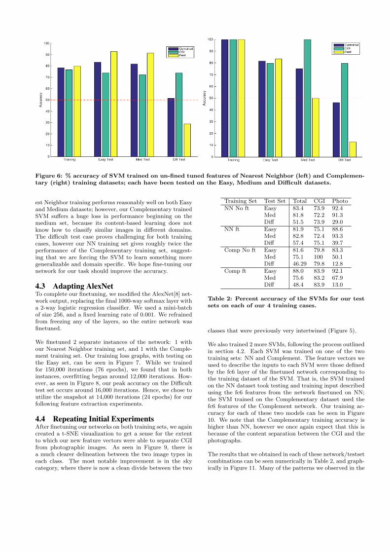
Figure 6: % accuracy of SVM trained on un-fined tuned features of Nearest Neighbor (left) and Complemen-tary (right) training datasets; each have been tested on the Easy, Medium and Difficult datasets.

est Neighbor training performs reasonably well on both Easyand Medium datasets; however, our Complementary trainedSVM suffers a huge loss in performance beginning on themedium set, because its content-based learning does notknow how to classify similar images in different domains.The difficult test case proves challenging for both trainingcases, however our NN training set gives roughly twice theperformance of the Complementary training set, suggest-ing that we are forcing the SVM to learn something moregeneralizable and domain specific. We hope fine-tuning ournetwork for our task should improve the accuracy.

4.3 Adapting AlexNetTo complete our finetuning, we modified the AlexNet[8] net-work output, replacing the final 1000-way softmax layer witha 2-way logistic regression classifier. We used a mini-batchof size 256, and a fixed learning rate of 0.001. We refrainedfrom freezing any of the layers, so the entire network wasfinetuned.

We finetuned 2 separate instances of the network: 1 withour Nearest Neighbor training set, and 1 with the Comple-ment training set. Our training loss graphs, with testing onthe Easy set, can be seen in Figure 7. While we trainedfor 150,000 iterations (76 epochs), we found that in bothinstances, overfitting began around 12,000 iterations. How-ever, as seen in Figure 8, our peak accuracy on the Difficulttest set occurs around 16,000 iterations. Hence, we chose toutilize the snapshot at 14,000 iterations (24 epochs) for ourfollowing feature extraction experiments.

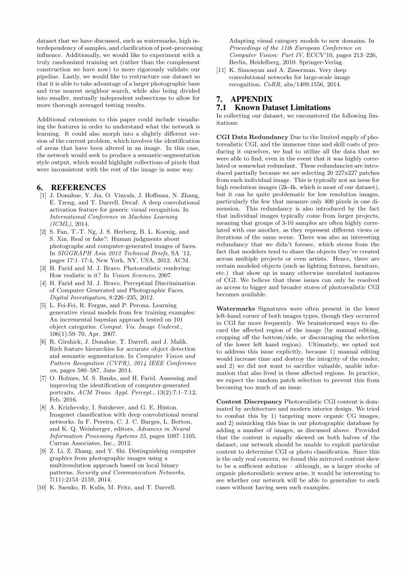
4.4 Repeating Initial ExperimentsAfter finetuning our networks on both training sets, we againcreated a t-SNE visualization to get a sense for the extentto which our new feature vectors were able to separate CGIfrom photographic images. As seen in Figure 9, there isa much clearer delineation between the two image types ineach class. The most notable improvement is in the skycategory, where there is now a clean divide between the two

Training Set Test Set Total CGI PhotoNN No ft Easy 83.4 73.9 92.4

Med 81.8 72.2 91.3Diff 51.5 73.9 29.0

NN ft Easy 81.9 75.1 88.6Med 82.8 72.4 93.3Diff 57.4 75.1 39.7

Comp No ft Easy 81.6 79.8 83.3Med 75.1 100 50.1Diff 46.29 79.8 12.8

Comp ft Easy 88.0 83.9 92.1Med 75.6 83.2 67.9Diff 48.4 83.9 13.0

Table 2: Percent accuracy of the SVMs for our testsets on each of our 4 training cases.

classes that were previously very intertwined (Figure 5).

We also trained 2 more SVMs, following the process outlinedin section 4.2. Each SVM was trained on one of the twotraining sets: NN and Complement. The feature vectors weused to describe the inputs to each SVM were those definedby the fc6 layer of the finetuned network corresponding tothe training dataset of the SVM. That is, the SVM trainedon the NN dataset took testing and training input describedusing the fc6 features from the network finetuned on NN;the SVM trained on the Complementary dataset used thefc6 features of the Complement network. Our training ac-curacy for each of these two models can be seen in Figure10. We note that the Complementary training accuracy ishigher than NN, however we once again expect that this isbecause of the content separation between the CGI and thephotographs.

The results that we obtained in each of these network/testsetcombinations can be seen numerically in Table 2, and graph-ically in Figure 11. Many of the patterns we observed in the

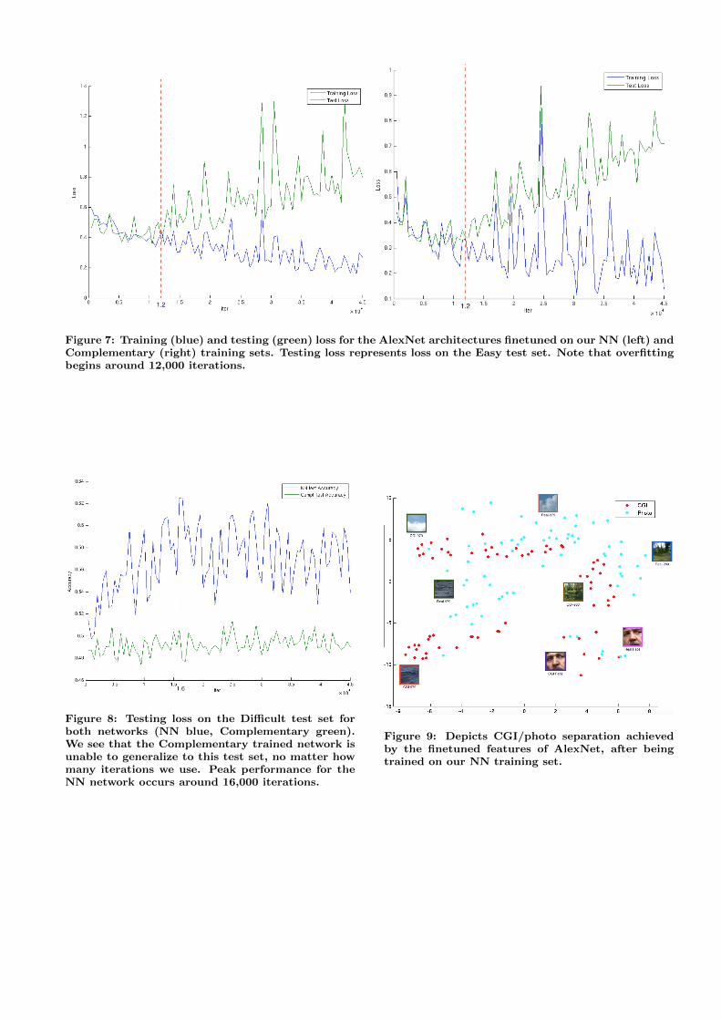
Figure 7: Training (blue) and testing (green) loss for the AlexNet architectures finetuned on our NN (left) andComplementary (right) training sets. Testing loss represents loss on the Easy test set. Note that overfittingbegins around 12,000 iterations.

Figure 8: Testing loss on the Difficult test set forboth networks (NN blue, Complementary green).We see that the Complementary trained network isunable to generalize to this test set, no matter howmany iterations we use. Peak performance for theNN network occurs around 16,000 iterations.

Figure 9: Depicts CGI/photo separation achievedby the finetuned features of AlexNet, after beingtrained on our NN training set.

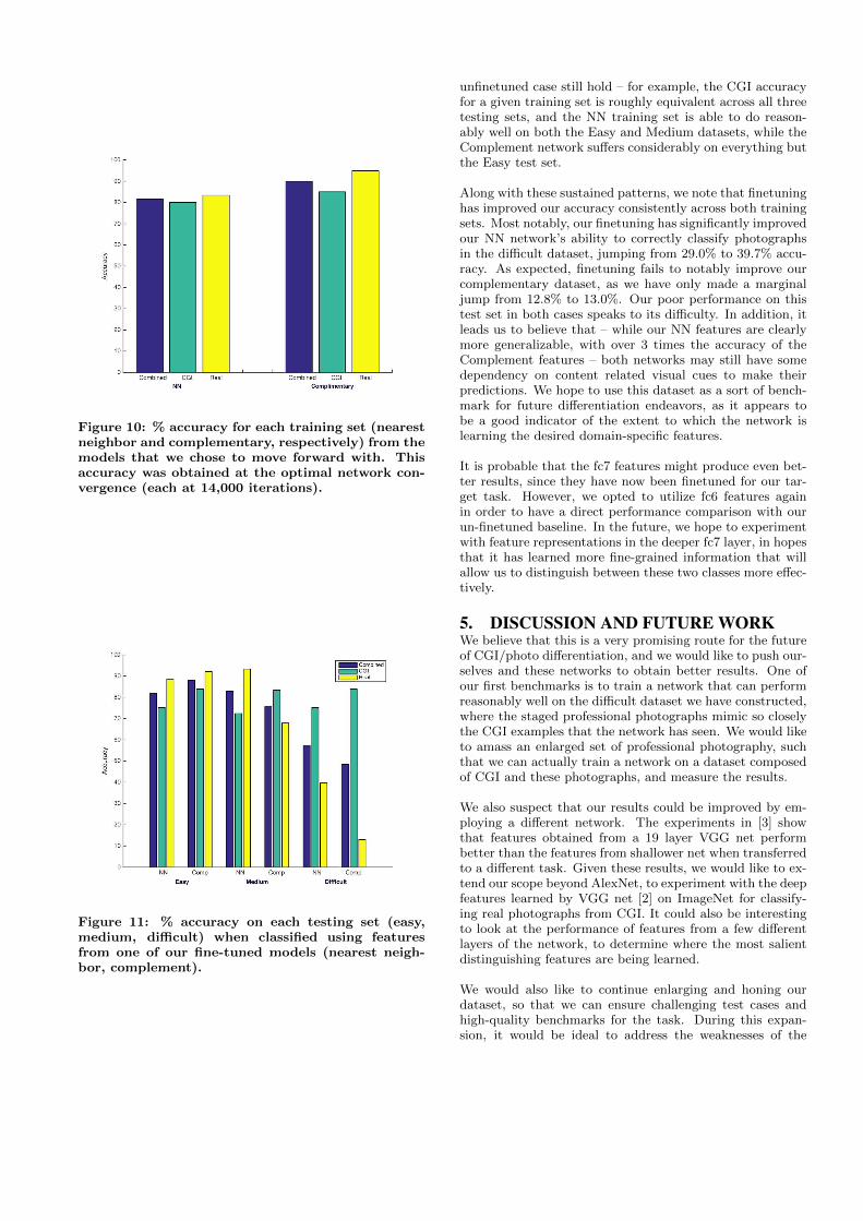
Figure 10: % accuracy for each training set (nearestneighbor and complementary, respectively) from themodels that we chose to move forward with. Thisaccuracy was obtained at the optimal network con-vergence (each at 14,000 iterations).

Figure 11: % accuracy on each testing set (easy,medium, difficult) when classified using featuresfrom one of our fine-tuned models (nearest neigh-bor, complement).

unfinetuned case still hold – for example, the CGI accuracyfor a given training set is roughly equivalent across all threetesting sets, and the NN training set is able to do reason-ably well on both the Easy and Medium datasets, while theComplement network suffers considerably on everything butthe Easy test set.

Along with these sustained patterns, we note that finetuninghas improved our accuracy consistently across both trainingsets. Most notably, our finetuning has significantly improvedour NN network’s ability to correctly classify photographsin the difficult dataset, jumping from 29.0% to 39.7% accu-racy. As expected, finetuning fails to notably improve ourcomplementary dataset, as we have only made a marginaljump from 12.8% to 13.0%. Our poor performance on thistest set in both cases speaks to its difficulty. In addition, itleads us to believe that – while our NN features are clearlymore generalizable, with over 3 times the accuracy of theComplement features – both networks may still have somedependency on content related visual cues to make theirpredictions. We hope to use this dataset as a sort of bench-mark for future differentiation endeavors, as it appears tobe a good indicator of the extent to which the network islearning the desired domain-specific features.

It is probable that the fc7 features might produce even bet-ter results, since they have now been finetuned for our tar-get task. However, we opted to utilize fc6 features againin order to have a direct performance comparison with ourun-finetuned baseline. In the future, we hope to experimentwith feature representations in the deeper fc7 layer, in hopesthat it has learned more fine-grained information that willallow us to distinguish between these two classes more effec-tively.

5. DISCUSSION AND FUTURE WORKWe believe that this is a very promising route for the futureof CGI/photo differentiation, and we would like to push our-selves and these networks to obtain better results. One ofour first benchmarks is to train a network that can performreasonably well on the difficult dataset we have constructed,where the staged professional photographs mimic so closelythe CGI examples that the network has seen. We would liketo amass an enlarged set of professional photography, suchthat we can actually train a network on a dataset composedof CGI and these photographs, and measure the results.

We also suspect that our results could be improved by em-ploying a different network. The experiments in [3] showthat features obtained from a 19 layer VGG net performbetter than the features from shallower net when transferredto a different task. Given these results, we would like to ex-tend our scope beyond AlexNet, to experiment with the deepfeatures learned by VGG net [2] on ImageNet for classify-ing real photographs from CGI. It could also be interestingto look at the performance of features from a few differentlayers of the network, to determine where the most salientdistinguishing features are being learned.

We would also like to continue enlarging and honing ourdataset, so that we can ensure challenging test cases andhigh-quality benchmarks for the task. During this expan-sion, it would be ideal to address the weaknesses of the

dataset that we have discussed, such as watermarks, high in-terdependency of samples, and clarification of post-processinginfluence. Additionally, we would like to experiment with atruly randomized training set (rather than the complementconstruction we have now) to more rigorously validate ourpipeline. Lastly, we would like to restructure our dataset sothat it is able to take advantage of a larger photographic baseand true nearest neighbor search, while also being dividedinto smaller, mutually independent subsections to allow formore thorough averaged testing results.

Additional extensions to this paper could include visualiz-ing the features in order to understand what the network islearning. It could also morph into a slightly different ver-sion of the current problem, which involves the identificationof areas that have been altered in an image. In this case,the network would seek to produce a semantic-segmentationstyle output, which would highlight collections of pixels thatwere inconsistent with the rest of the image in some way.

6. REFERENCES[1] J. Donahue, Y. Jia, O. Vinyals, J. Hoffman, N. Zhang,

E. Tzeng, and T. Darrell. Decaf: A deep convolutionalactivation feature for generic visual recognition. InInternational Conference in Machine Learning(ICML), 2014.

[2] S. Fan, T.-T. Ng, J. S. Herberg, B. L. Koenig, andS. Xin. Real or fake?: Human judgments aboutphotographs and computer-generated images of faces.In SIGGRAPH Asia 2012 Technical Briefs, SA ’12,pages 17:1–17:4, New York, NY, USA, 2012. ACM.

[3] H. Farid and M. J. Bravo. Photorealistic rendering:How realistic is it? In Vision Sciences, 2007.

[4] H. Farid and M. J. Bravo. Perceptual Discriminationof Computer Generated and Photographic Faces.Digital Investigation, 8:226–235, 2012.

[5] L. Fei-Fei, R. Fergus, and P. Perona. Learninggenerative visual models from few training examples:An incremental bayesian approach tested on 101object categories. Comput. Vis. Image Underst.,106(1):59–70, Apr. 2007.

[6] R. Girshick, J. Donahue, T. Darrell, and J. Malik.Rich feature hierarchies for accurate object detectionand semantic segmentation. In Computer Vision andPattern Recognition (CVPR), 2014 IEEE Conferenceon, pages 580–587, June 2014.

[7] O. Holmes, M. S. Banks, and H. Farid. Assessing andimproving the identification of computer-generatedportraits. ACM Trans. Appl. Percept., 13(2):7:1–7:12,Feb. 2016.

[8] A. Krizhevsky, I. Sutskever, and G. E. Hinton.Imagenet classification with deep convolutional neuralnetworks. In F. Pereira, C. J. C. Burges, L. Bottou,and K. Q. Weinberger, editors, Advances in NeuralInformation Processing Systems 25, pages 1097–1105.Curran Associates, Inc., 2012.

[9] Z. Li, Z. Zhang, and Y. Shi. Distinguishing computergraphics from photographic images using amultiresolution approach based on local binarypatterns. Security and Communication Networks,7(11):2153–2159, 2014.

[10] K. Saenko, B. Kulis, M. Fritz, and T. Darrell.

Adapting visual category models to new domains. InProceedings of the 11th European Conference onComputer Vision: Part IV, ECCV’10, pages 213–226,Berlin, Heidelberg, 2010. Springer-Verlag.

[11] K. Simonyan and A. Zisserman. Very deepconvolutional networks for large-scale imagerecognition. CoRR, abs/1409.1556, 2014.

7. APPENDIX7.1 Known Dataset LimitationsIn collecting our dataset, we encountered the following lim-itations:

CGI Data Redundancy Due to the limited supply of pho-torealistic CGI, and the immense time and skill costs of pro-ducing it ourselves, we had to utilize all the data that wewere able to find, even in the event that it was highly corre-lated or somewhat redundant. These redundancies are intro-duced partially because we are selecting 20 227x227 patchesfrom each individual image. This is typically not an issue forhigh resolution images (2k-4k, which is most of our dataset),but it can be quite problematic for low resolution images,particularly the few that measure only 400 pixels in one di-mension. This redundancy is also introduced by the factthat individual images typically come from larger projects,meaning that groups of 3-10 samples are often highly corre-lated with one another, as they represent different views oriterations of the same scene. There was also an interestingredundancy that we didn’t foresee, which stems from thefact that modelers tend to share the objects they’ve createdacross multiple projects or even artists. Hence, there arecertain modeled objects (such as lighting fixtures, furniture,etc.) that show up in many otherwise unrelated instancesof CGI. We believe that these issues can only be resolvedas access to bigger and broader stores of photorealistic CGIbecomes available.

Watermarks Signatures were often present in the lowerleft-hand corner of both images types, though they occurredin CGI far more frequently. We brainstormed ways to dis-card the affected region of the image (by manual editing,cropping off the bottom/side, or discouraging the selectionof the lower left hand region). Ultimately, we opted notto address this issue explicitly, because 1) manual editingwould increase time and destroy the integrity of the render,and 2) we did not want to sacrifice valuable, usable infor-mation that also lived in these affected regions. In practice,we expect the random patch selection to prevent this frombecoming too much of an issue.

Content Discrepancy Photorealistic CGI content is dom-inated by architecture and modern interior design. We triedto combat this by 1) targeting more organic CG images,and 2) mimicking this bias in our photographic database byadding a number of images, as discussed above. Providedthat the content is equally skewed on both halves of thedataset, our network should be unable to exploit particularcontent to determine CGI or photo classification. Since thisis the only real concern, we found this mirrored content skewto be a sufficient solution – although, as a larger stocks oforganic photorealistic scenes arise, it would be interesting tosee whether our network will be able to generalize to suchcases without having seen such examples.

Suboptimal Nearest Neighbor Our preliminary classifi-cation of the images could result in suboptimal patch matches,because each patch is limited in the number of potential can-didates it can consider. This is particularly relevant if somesub-section of the original image differs drastically from theoverarching semantic content (i.e., a plant in the midst ofan indoor scene), because our preemptive classification mayhave separated this patch from its actual closest match. Inthe future, we may attempt to rerun nearest neighbor searchwithout this preliminary filtering to see if our results im-prove. However, the purpose of this matching is just to en-sure that our network has challenging examples to learn on,and our visualizations seem to corroborate that our matchesare satisfactory for this purpose. As such, we are not cer-tain that it would be worth the additional time complexity;however, it may be worth exploring.

Ambiguous Origins and Processing While we inten-tionally selected images that were well-tagged and locatedon sites specifically tailored to a particular category (CGIor photographic), it is impossible to be 100% positive thatthese labels are correct since we had no involvement in thecreation process. There are also semi-ambiguous definitionsfor ”CGI” and ”photograph”, which made it difficult to en-sure that even reasonably labeled data was of a consistentform. For instance, we have not specified to what degreepost-processing is allowed to be present in our samples. Itis very rare that images are left untouched after being re-turned from the camera or renderer, but the exact range ofalterations that are represented in our dataset is unknown.Similarly, we did not address whether CG images containingphotographic elements (as backgrounds, etc.) would be per-mitted. In reality, it would be nearly impossible to imposesuch restrictions. There are also different ways to producesuch images: for instance, photoshopping the pre-renderedobjects onto the photographic backgrounds, versus insertingthe image into the modeled scene and rendering this texturealong with the rest of the image directly. Each of these islikely to have dramatically different pixel-level properties,but these production details are rarely specified and to theuntrained eye they may be equally convincing. Short of ex-plicitly stating such preferences and constructing the datasamples ourselves to reflect them, we are unsure of a reason-able way to combat these issues.